Quantization of the Interacting Non-Hermitian Higher Order Derivative Field

Abstract.

The quantization of higher order time derivative theories including interactions is unclear. In this paper in order to solve this problem, we propose to consider a complex version of the higher order derivative theory and map this theory to a real first order theory. To achieve this relationship, the higher order derivative formulation must be complex since there is not a real canonical transformation from this theory to a real first order theory with stable interactions. In this manner, we work with a non-Hermitian higher order time derivative theory. To quantize this complex theory, we introduce reality conditions that allow us to map the complex higher order theory to a real one, and we show that the resulting theory is regularizable and renormalizable for a class of interactions.

1. Introduction

In physics and mathematics it has been developed some methods for facing up problems by means of applying an extension of the real space to the complex plane. In quantum mechanics, electrodynamics, quantum field theory and differential equations is common knowledge. Methods for solving differential equations are narrowly linked to the higher order derivative mechanics [1] which results in an interest by encoding the higher order theories to the usual first order mechanics. These theories have both Lagrangian and Hamiltonian formulations, and using the latter is, in principle, possible to quantize the system. The key issue is that it hasn’t achieved an acceptable full quantization of interacting higher order derivative theories [2, 3]. One always has negative probabilities, energies unbounded below or a non-unitary dispersion matrix.

Though it appears which the higher order theories aren’t a fundamental theme, many works have showed that using these theories fundamental problems could be solved. Examples where these theories arise is F(R) theories, in special the formulation given by Stelle [4] in which it is aggregated a higher order derivative term that allow to obtain a renormalizable theory, bounded by the nature of higher order derivative theories.

Other example is the bosonization proposed by Schwinger [5] for the electrodynamics in 2 dimensions in which using a non-local transformation it is possible arrive from usual electrodynamics to the higher order derivative theory with a bosonic field.

The quantization of the higher order derivative theories isn’t a trivial issue. As early as 1950, Pais and Uhlenbeck established a non-local transformation that map from a real higher order derivative theory to the Hamiltonian of two oscillators, with one of the oscillators with opposite sign in the kinetic term [6]. A subsequent analysis showed that the mapping described by Pais-Uhlenbeck point out an inconsistent quantization with problems as negative probabilities, energy unbounded from below and a non-unitary dispersion matrix [7]. However, Smilga showed that if the Pais-Uhlenbeck model is free and it has different masses, the inconsistencies don’t exist in a quantum theory, but if masses are equal, Jordan blocks appear implying the loss of unitarity [2]. Subsequent to the Pais-Uhlenbeck model, in 1975 Bernard and Duncan [8], proposed a field theory model with higher order time derivatives which they try to quantize using path integrals. Proceeding in this way it was possible to show that the Matthew’s theorem is applicable [8]. From a model with different masses Hawking and Hertog proposed that the real Bernard-Duncan model is set in two independent Hilbert spaces and resulting that the real higher order derivative theory is acceptable if it is free [9]. In spite of the free Bernard-Duncan model is quantizable, a way of including interaction potentials is unfinished still, due to the presence of negative norm states [10].

The above analysis suggest that the axioms of quantum mechanics aren’t sufficient to establish a consistent quantization for the higher order derivative theories. In special the Hermiticity axiom for these theories result incompatible with a higher order derivative field. Regarding about, a non-Hermitian theory was proposed by Bender and Manheim [11], who explored this possibility exploiting the $\mathcal{PT}$-symmetry in order to determine if a mapping from non-Hermitian theory to Hermitian theory is possible. For the construction of this non-Hermitian formulation it is necessary to introduce a new inner product which define a new $\mathcal{PT}$-quantum mechanics. This suggest the idea of applying a imaginary scaling transformation that allow to avoid non-Hermitian $\mathcal{PT}$-symmetric operators [3]. Similar to this is to apply a complex canonical transformation directly [12] considering the reality conditions [13]. In parallel with this work, it is possible to introduce interactions in the higher order model using the reality conditions and to develop the complex structure for higher order derivative mechanics.

The purpose of this work is to show the equivalence between a complex higher order derivative theory with interactions and a real first order theory with two scalar fields. The equivalence is established using reality conditions that cancel the additional degrees of freedom and map from the complex to the real space.

The higher order derivative theory used as an example is a complexification of the Bernard-Duncan model [8]. To start a quantization by annihilation and creation operators is established. In that context, using annihilation and creation operators and the reality conditions, we show the possible interaction potentials that result in a potential with a stable critical point.

This paper is organized as follows. Section 2 introduces the key problem of the higher order derivative theories using the Bernard-Duncan model. After that, we discuss the reality conditions by means of a simple example given by Ashtekar [13]. Section 3 presents the complex Bernard-Duncan theory using higher order derivative fields. These fields allow to map from a complex theory to a real theory and the corresponding reality conditions appear into the complex theory. A Fourier transform let, by means of the higher order derivative fields, to define annihilation and creation operators. In this part, the reality conditions are defined in terms of fields. In Section 4 we apply the reality conditions in fields by means of annihilation and creation operators and the commutation relations between annihilation and creation operators are established. The higher order derivative Hamiltonian density is found in terms of these operators using the reality conditions. Finally, we establish a relation between the complex higher order Hamiltonian theory that includes the reality conditions and the Hamiltonian theory of two real Klein-Gordon fields. In Section 5, the interaction potentials are described so that using the reality conditions, it is obtained a stable interaction with a critic point that allows to do a perturbative expansion and we show that the resulting theory is regularizable and renormalizable. Finally, in Section 6 we summarize our results.

2. Creation and Annihilation Operators in the real theory

In order to analyze problems that appear when we quantize a higher order temporal derivative theory, we introduce the Bernard-Duncan model [8] by means of its real Lagrangian density

(2.1) $$\mathcal{L}_{BD}=-\frac{1}{2}(\partial_{\mu}\partial^{\mu}\varphi)^{2}+\frac{(m_{1}^{2}+m_{2}^{2})}{2}\partial_{\mu}\varphi\partial^{\mu}\varphi-\frac{m_{1}^{2}m_{2}^{2}}{2}\varphi^{2},$$

which generates the equation of motion

(2.2) $$\Box^{2}\varphi+(m_{1}^{2}+m_{2}^{2})\Box\varphi+m_{1}^{2}m_{2}^{2}\varphi=0.$$

Using the Lagrangian density (2.1) and the Ostrogradsky theory [1], we obtain the higher order derivative momenta for the fields $\varphi$ and $\dot{\varphi}$

(2.3) $$\pi_{\dot{\varphi}}=-\Box\varphi,$$

$$\pi_{\varphi}=\varphi^{(3)}-\nabla^{2}\frac{d}{dt}\varphi+(m_{1}^{2}+m_{2}^{2})\frac{d}{dt}\varphi.$$

The above equations will allow to define a symplectic structure of the phase space considering that the real Lagrangian depends on $(\varphi,\dot{\varphi},\ddot{\varphi})$.

Using the Fourier transform

(2.4) $$\varphi(\vec{x},t)=\int\!\frac{d^{3}p}{(2\pi)^{\frac{3}{2}}}e^{i\vec{p}\cdotp\vec{x}}\Psi(\vec{p},t),$$

the equation of motion (2.2) results

(2.5) $$\Psi^{(4)}(\vec{p},t)+(E_{1}^{2}+E_{2}^{2})\Psi^{(2)}(\vec{p},t)+E_{1}^{2}E_{2}^{2}\Psi(\vec{p},t)=0.$$

The general solution to (2.5) is

(2.6) $$\Psi(\vec{p},t)=\textbf{{a}}(\vec{p})e^{-iE_{1}t}+\textbf{{c}}(-\vec{p})e^{iE_{1}t}+\textbf{{b}}(\vec{p})e^{-iE_{2}t}+\textbf{{d}}(-\vec{p})e^{iE_{2}t}.$$

In the standard formalism is requested that the Lagrangian density to be real. In consequence, the field $\varphi(\vec{x},t)$ must be real which imposes a restriction in the Fourier coefficients

(2.7) $$\textbf{{d}}=\textbf{{b}}^{*},\qquad\textbf{{c}}=\textbf{{a}}^{*}.$$

With the real solution of the field for (2.2), we obtain hermiticity when a quantization is done by means of promote the Fourier coefficients to operators.

The solution which include (2.7), which obey (2.5) and which induce a real $\varphi$ in (2.4) is

(2.8) $$\Psi(\vec{p},t)=\textbf{{a}}(\vec{p})e^{-iE_{1}t}+\textbf{{a}}^{*}(-\vec{p})e^{iE_{1}t}+\textbf{{b}}(\vec{p})e^{-iE_{2}t}+\textbf{{b}}^{*}(-\vec{p})e^{iE_{2}t}.$$

In order to quantize the system and following the usual rules, we promote coefficients a and b to operators, the general solution to (2.2) is

$$\varphi(\vec{x},t)=\int\frac{d^{3}p}{(2\pi)^{\frac{3}{2}}}\left\{\frac{1}{(2E_{1})^{\frac{1}{2}}(m_{2}^{2}-m_{1}^{2})^{\frac{1}{2}}}[\textbf{{a}}(\vec{p})e^{i\vec{p}\cdotp\vec{x}-iE_{1}t}+\textbf{{a}}^{\dagger}(\vec{p})e^{-i\vec{p}\cdotp\vec{x}+iE_{1}t}]\right.$$

(2.9) $$\left.+\frac{1}{(2E_{2})^{\frac{1}{2}}(m_{2}^{2}-m_{1}^{2})^{\frac{1}{2}}}[\textbf{{b}}(\vec{p})e^{i\vec{p}\cdotp\vec{x}-iE_{2}t}+\textbf{{b}}^{\dagger}(\vec{p})e^{-i\vec{p}\cdotp\vec{x}+iE_{2}t}]\right\},$$

and from this expression, we obtain the reality condition $\varphi=\varphi^{\dagger}$, which implies that the field $\varphi$ is hermitic. The solution (2) is Lorentz invariant and it makes sense only in the case $m_{2}\neq m_{1}$, along this article we will use this condition.

The case $m_{1}=m_{2}$ has been analyzed in [11] and we can use similar arguments. However, from (2) is possible to find $\dot{\varphi}$ that is a field in the Ostrogradsky’s theory and to obtain the momenta (2.3) in terms of annihilation and creation operators.

The commutators associated to the annihilation and the creation operators resulting from the canonical commutators are

(2.10) $$[\textbf{{a}}(\vec{p}),\textbf{{a}}^{\dagger}(\vec{p^{\prime}})]=\delta(\vec{p}-\vec{p^{\prime}}),$$

(2.11) $$\ [\textbf{{b}}(\vec{p}),\textbf{{b}}^{\dagger}(\vec{p^{\prime}})]=-\delta(\vec{p}-\vec{p^{\prime}}).$$

The sign in the commutation relation (2.11) is the root of the problem to quantize the higher order derivative theories.

For example, considering the higher order derivative theory in (2.1), we get the Hamiltonian density by means of the Ostrogradsky method

(2.12) $$\mathcal{H}_{BD}=\pi_{\varphi}\frac{d\varphi}{dt}+\pi_{\dot{\varphi}}\frac{d^{2}\varphi}{dt^{2}}-\mathcal{L}_{BD},$$

with the Hamiltonian density given by

(2.13) $$\mathcal{H}_{BD}=\pi_{\varphi}\dot{\varphi}-\frac{1}{2}\pi^{2}_{\dot{\varphi}}-\frac{(m_{1}^{2}+m_{2}^{2})}{2}\dot{\varphi}^{2}+\frac{m_{1}^{2}m_{2}^{2}}{2}\varphi^{2}+\pi_{\dot{\varphi}}\nabla^{2}\varphi+\frac{(m_{1}^{2}+m_{2}^{2})}{2}(\nabla\varphi)^{2}$$

and with the respective phase space $(\varphi,\pi_{\varphi},\dot{\varphi},\pi_{\dot{\varphi}})$.

In terms of annihilation and creation operators the Hamiltonian density (2.13) that is obtained by Ostrogradsky’s method (2.12) is unbounded from below and results

(2.14) $$\ \ H_{BD}=\int d^{3}p\left\{\frac{E_{1}}{2}[\textbf{{a}}^{\dagger}(\vec{p})\textbf{{a}}(\vec{p})+\textbf{{a}}(\vec{p})\textbf{{a}}^{\dagger}(\vec{p})]-\frac{E_{2}}{2}[\textbf{{b}}^{\dagger}(\vec{p})\textbf{{b}}(\vec{p})+\textbf{{b}}(\vec{p})\textbf{{b}}^{\dagger}(\vec{p})]\right\}.$$

The commutators (2.11) generate negative norm states or negative probabilities, so this theory isn’t a good quantum theory. Because, there isn’t an interaction potential here and the free system doesn’t interchange energy from one field to another field, so it is correct to think that the system can be divided in two independent free systems [9]. However, the self-energy contribution manifest an internal interaction in the system which is induced by an external agent so consequently, a system without a self-interaction potential is a non-physical system. To establish in the Bernard-Duncan model an interaction potential, that can be handled using perturbative theory, using the approach (2.14) is impossible. For that reason, we think that is necessary to relax the Hermiticity condition for $\varphi$ that is to say $\varphi(x)\neq\varphi^{\dagger}$. The idea of a reality conditions exposed by Ashtekar in the case of gravitation [13] is to replace the Hermiticity condition in order to set a new Hermiticity condition least restrictive which allows a complex higher order derivative field and a possible solution to the problem in (2.14). In the next subsection, we will review this strategy.

2.1. Reality Conditions

The complexification by means of an extended space is a traditional method in mathematics and physics which is used to solve several problems in different branches of the science. In our case, we don’t focus in the complexification, but we focus in reality conditions which allow to reduce and to solve a problem by means of projecting to the real space. It is possible to understand the complexification as an extension of the physical degrees of freedom and after that to build a projection from the complex to the real space. Bender proposed a similar situation [11], changing the internal product using the PT symmetry as an assistance to find the correct internal product. In our case the reality conditions will provide the appropriate projection and also the internal product. To introduce this proposal, we consider a simple example that allows to illustrate some consequences of using this method.

Let us consider the harmonic oscillator with phase space $\Gamma=(q,p)$ in two dimensions and a real Hamiltonian

(2.15) $$h(q,p)=\frac{1}{2}(q^{2}+p^{2}).$$

Now, we want to extend the domain of definition to the complex space, then a new variable is used

(2.16) $$z\equiv q-ip,$$

where the pair $\tilde{\Gamma}=(q,z)$, is the new complex phase space, with Poisson brackets defined by

(2.17) $$\left\{q,q\right\}=0,\qquad\left\{z,z\right\}=0,\qquad\left\{z,q\right\}=i,$$

which will be thought as a canonical conjugate set. Introducing a function $f(q,p)$ on $\Gamma$ is possible to define a new function on $\tilde{\Gamma}$ using (2.16)

(2.18) $$g(q,z)\equiv f(q,i(z-q))$$

and any function can be constructed in this way, taking care of computing the evolution by means of the Poisson brackets (2.17).

In particular the Hamiltonian function in terms of $(q,z)$ is

(2.19) $$h(q,z)=\frac{1}{2}(q^{2}-(z-q)^{2})=zq-\frac{1}{2}z^{2}$$

and using commutators the temporal evolution is

(2.20) $$\dot{q}=\left\{q,h\right\}=iz-iq,\qquad\dot{z}=\left\{z,h\right\}=iz.$$

The equations (2.20) are equations of motion for the complex phase space $\tilde{\Gamma}$. However, this description have to be consistent with the equations of motion resulting from (2.15) in order to preserve the original dynamics. Now, to project from the complex space $(q,z)$ to the original real space we propose the following reality conditions

(2.21) $$q=q^{*},\qquad z^{*}=(-z+2q).$$

The first equation in (2.21) set a real $q$ and it is similar to the initial real phase space. On the other hand the second equation recovers the initial real phase space preserving $p=p^{*}$. This conditions impose a constraint for $z$ in the new complex phase space.

To put it briefly, we have first a mapping from a real phase space to a complex space and in order to make a consistent theory and a compatible dynamics, we introduce the reality conditions (2.21) on $\tilde{\Gamma}$.

Note that the relationship (2.16) obeys the reality conditions and provide a direct mapping which carries from the equations of motion (2.20) to the equations of motion generated by (2.15). The above idea will be applied in the Complex Bernard Duncan model.

3. Complex Bernard-Duncan Theory and Reality conditions

There are a lot of higher order derivative field theories, but in order to understand their characteristics, we choose the most simplest the Bernard-Duncan model.

In this section it will be analyzed the consequence of extending the field theory (2.1) to the complex plane, i.e. we consider that the field $\phi$ is defined by

(3.1) $$\phi\equiv\phi_{R}+i\phi_{I},$$

with the complex higher order derivative action given by

(3.2) $$W=\int\!d^{4}x\frac{1}{2}[-(\Box\phi)^{2}+(m_{1}^{2}+m_{2}^{2})\partial_{\mu}\phi\partial^{\mu}\phi-m_{1}^{2}m_{2}^{2}\phi^{2}].$$

From the expression (3.2), it is possible to make a variation in $\phi$ and we obtain

(3.3) $$\delta W=\int\!d^{4}x-\frac{\partial^{2}}{\partial t^{2}}(\Box\phi)\delta\phi+(\Box\phi)\nabla^{2}\delta\phi-(m_{1}^{2}+m_{2}^{2})\frac{d^{2}}{dt^{2}}\phi\delta\phi$$

$$-(m_{1}^{2}+m_{2}^{2})\nabla\phi\cdotp\delta\nabla\phi-m_{1}^{2}m_{2}^{2}\phi\delta\phi$$

$$+\int\!d^{3}x-\Box\phi\delta\frac{d}{dt}\phi+(m_{1}^{2}+m_{2}^{2})\frac{d}{dt}\phi\delta\phi-\frac{d}{dt}(-\Box\phi)\delta\phi.$$

From the last expression, we obtain the momenta

(3.4) $$\pi_{\dot{\phi}}=-\Box\phi,$$

$$\pi_{\phi}=\phi^{(3)}-\nabla^{2}\frac{d}{dt}\phi+(m_{1}^{2}+m_{2}^{2})\frac{d}{dt}\phi$$

then the variation of the action can be summarized as

(3.5) $$\delta W=\int\!d^{4}x-[\Box^{2}\phi+(m_{1}^{2}+m_{2}^{2})\Box\phi+m_{1}^{2}m_{2}^{2}\phi]\delta\phi+\int\!d^{3}x[\pi_{\dot{\phi}}\delta\dot{\phi}+\pi_{\phi}\delta\phi].$$

The complex equation of motion can be identified from (3.5)

(3.6) $$\Box^{2}\phi+(m_{1}^{2}+m_{2}^{2})\Box\phi+m_{1}^{2}m_{2}^{2}\phi=0$$

and using the Fourier transformation (2.4) applied to this case, we obtain

(3.7) $$\psi^{(4)}(\vec{p},t)+(E_{1}^{2}+E_{2}^{2})\psi^{(2)}(\vec{p},t)+E_{1}^{2}E_{2}^{2}\psi(\vec{p},t)=0,$$

where $E_{1}^{2}=(\vec{p}^{2}+m_{1}^{2})$ and $E_{2}^{2}=(\vec{p}^{2}+m_{2}^{2})$ are two energies with different masses. In this case the field $\phi$ is complex then to determine $\psi$, we use a new set of reality conditions.

These conditions will cancel the additional degrees of freedom that appear from the complexification of the system. The equation (3.7) can be rewritten as

(3.8) $$\left(\frac{d^{2}}{dt^{2}}+E_{1}^{2}\right)\left(\frac{d^{2}}{dt^{2}}+E_{2}^{2}\right)\psi(\vec{p},t)=0$$

and the general solution is

(3.9) $$\psi(\vec{p},t)=\textbf{f}(\vec{p})e^{-iE_{1}t}+\textbf{c}(-\vec{p})e^{iE_{1}t}+\textbf{b}(\vec{p})e^{-iE_{2}t}+\textbf{d}(-\vec{p})e^{iE_{2}t}.$$

In particular, we look for a Lorentz invariant solution to (3.6) which is

(3.10) $$\phi(\vec{x},t)=\int\!\frac{d^{3}p}{(2\pi)^{\frac{3}{2}}}\frac{1}{(2E_{1})^{\frac{1}{2}}}[\textbf{f}(\vec{p})e^{i\vec{p}\cdotp\vec{x}-iE_{1}t}+\textbf{c}(\vec{p})e^{-i\vec{p}\cdotp\vec{x}+iE_{1}t}]$$

$$+\frac{1}{(2E_{2})^{\frac{1}{2}}}[\textbf{b}(\vec{p})e^{i\vec{p}\cdotp\vec{x}-iE_{2}t}+\textbf{d}(\vec{p})e^{-i\vec{p}\cdotp\vec{x}+iE_{2}t}]$$

and using this field, we obtain $\dot{\phi}$ and the corresponding momenta in the Ostrogradsky formulation $\pi_{\phi}$, $\pi_{\dot{\phi}}$ that impose a relationship between the complex fields and momenta with the annihilation and creation operators.

With the new fields and momenta (3.4) the resulting Hamiltonian density is

$$\mathcal{H}_{BD}=\pi_{\phi}\dot{\phi}-\frac{(\pi_{\dot{\phi}})^{2}}{2}-\frac{(m_{1}^{2}+m_{2}^{2})}{2}\dot{\phi}^{2}+\frac{(m_{1}^{2}+m_{2}^{2})}{2}(\nabla\phi)^{2}+\frac{m_{1}^{2}m_{2}^{2}}{2}\phi^{2}$$

(3.11) $$-\nabla\phi\cdotp\nabla(\pi_{\dot{\phi}}).$$

The Hamiltonian density (3) is similar to (2.13), but (3) is complex while the density (2.13) is real and different from (3) by a total spatial derivative.

Following the idea of Section 2.1, we introduce a mapping from the complex to the real space. To define this mapping, we implement a canonical transformation between the complex phase space $(\phi,\dot{\phi},\pi_{\phi},\pi_{\dot{\phi}})$ to the real phase space $(\psi_{1},\pi_{\psi_{1}},\psi_{2},\pi_{\psi_{2}})$ defined as

(3.12) $$\psi_{1}=\frac{1}{(m_{1}^{2}-m_{2}^{2})^{\frac{1}{2}}}(im_{2}^{2}\phi-i\pi_{\dot{\phi}}),\qquad\psi_{2}=\frac{1}{(m_{1}^{2}-m_{2}^{2})^{\frac{1}{2}}}(m_{1}^{2}\phi-\pi_{\dot{\phi}}),$$

$$\pi_{\psi_{1}}=i\frac{1}{(m_{1}^{2}-m_{2}^{2})^{\frac{1}{2}}}(\pi_{\phi}-m_{1}^{2}\dot{\phi}),\qquad\pi_{\psi_{2}}=\frac{1}{(m_{1}^{2}-m_{2}^{2})^{\frac{1}{2}}}(\pi_{\phi}-m_{2}^{2}\dot{\phi})$$

which is a local and linear canonical transformation. In order to fully establish that the fields $\psi_{1}$ and $\psi_{2}$ and the respective momenta $\pi_{\psi_{1}},\pi_{\psi_{2}}$, are real we assume that are complex fields and impose that the imaginary parts are zero.

The real and imaginary parts of the complex fields and the complex momenta are

$$(\psi_{1R}+i\psi_{1I})=\frac{1}{(m_{1}^{2}-m_{2}^{2})^{\frac{1}{2}}}[(\pi_{\dot{\phi}_{I}}-m_{2}^{2}\phi_{I})-i(\pi_{\dot{\phi}_{R}}-m_{2}^{2}\phi_{R})],$$

$$(\psi_{2R}+i\psi_{2I})=\frac{1}{(m_{1}^{2}-m_{2}^{2})^{\frac{1}{2}}}[(m_{1}^{2}\phi_{R}-\pi_{\dot{\phi}_{R}})-i(\pi_{\dot{\phi}_{I}}-m_{1}^{2}\phi_{I})],$$

$$(\pi_{\psi_{1R}}+i\pi_{\psi_{1I}})=\frac{1}{(m_{1}^{2}-m_{2}^{2})^{\frac{1}{2}}}[-(\pi_{\phi_{I}}-m_{1}^{2}\dot{\phi}_{I})+i(\pi_{\phi_{R}}-m_{1}^{2}\dot{\phi}_{R})],$$

(3.13) $$(\pi_{\psi_{2R}}+i\pi_{\psi_{2I}})=\frac{1}{(m_{1}^{2}-m_{2}^{2})^{\frac{1}{2}}}[(\pi_{\phi_{R}}-m_{2}^{2}\dot{\phi}_{R})+i(\pi_{\phi_{I}}-m_{2}^{2}\dot{\phi}_{I})].$$

Therefore, the equations (3) impose 4 conditions

(3.14) $$(\pi_{\dot{\phi}_{R}}-m_{2}^{2}\phi_{R})=0,\qquad(\pi_{\dot{\phi}_{I}}-m_{1}^{2}\phi_{I})=0,$$

$$(\pi_{\phi_{R}}-m_{1}^{2}\dot{\phi}_{R})=0,\qquad(\pi_{\phi_{I}}-m_{2}^{2}\dot{\phi}_{I})=0,$$

these are the reality conditions for the complex fields $(\phi,\dot{\phi},\pi_{\phi},\pi_{\dot{\phi}})$.

Using these conditions, the relationship between components of the complex fields and the fields $(\psi_{1},\psi_{2},\pi_{\psi_{1}},\pi_{\psi_{2}})$ are

(3.15) $$\psi_{2}=(m_{1}^{2}-m_{2}^{2})^{\frac{1}{2}}\phi_{R},\qquad\psi_{1}=(m_{1}^{2}-m_{2}^{2})^{\frac{1}{2}}\phi_{I},$$

(3.16) $$\pi_{\psi_{2}}=(m_{1}^{2}-m_{2}^{2})^{\frac{1}{2}}\dot{\phi}_{R},\qquad\pi_{\psi_{1}}=(m_{1}^{2}-m_{2}^{2})^{\frac{1}{2}}\dot{\phi}_{I}.$$

In addition to the above issues we work in the Hamiltonian formulation because it is easy to define a complex canonical transformation (3.12) instead of a non local complex transformation that is defined in the Lagrangian formulation [12]. In terms of the Lagrangian formulation, the non local complex transformation point out troubles as linearity, and simultaneity. However we wish to remark by means of the Hamiltonian formulation that it is possible to introduce a consistent theory including a Lagrangian formulation using a Legendre transformation.

In (3), we impose that the fields $(\psi_{1},\pi_{\psi_{2}},\psi_{2},\pi_{\psi_{2}},)$ are real, these conditions constraint the complex higher order fields $(\phi,\pi_{\phi},\dot{\phi},\pi_{\dot{\phi}})$, then we want to rewrite these conditions in terms of the higher order fields and their complex conjugate fields so we get the expressions

$$(m_{1}^{2}-m_{2}^{2})\phi^{*}=(m_{1}^{2}+m_{2}^{2})\phi-2\pi_{\dot{\phi}}$$

$$(m_{1}^{2}-m_{2}^{2})\dot{\phi}^{*}=-(m_{1}^{2}+m_{2}^{2})\dot{\phi}+2\pi_{\phi}$$

$$(m_{1}^{2}-m_{2}^{2})\pi^{*}_{\phi}=(m_{1}^{2}+m_{2}^{2})\pi_{\phi}-2m_{1}^{2}m_{2}^{2}\dot{\phi}$$

(3.17) $$(m_{1}^{2}-m_{2}^{2})\pi^{*}_{\dot{\phi}}=-(m_{1}^{2}+m_{2}^{2})\pi_{\dot{\phi}}+2m_{1}^{2}m_{2}^{2}\phi.$$

In this way, starting with a complex higher order theory, using a canonical transformation and applying the reality conditions we were able to reduce the complex theory to a real one.

Now, we need to figure out the nature of the dynamics of the new fields $(\psi_{1},\psi_{2},\pi_{\psi_{1}},\pi_{\psi_{2}})$. To do that we compute the Hamiltonian density (3) in terms of these fields and we get

(3.18) $$\mathcal{H}_{KG}=\frac{\pi^{2}_{\psi_{1}}}{2}+\frac{(\nabla\psi_{1})^{2}}{2}+\frac{m_{1}^{2}\psi_{1}^{2}}{2}+\frac{\pi^{2}_{\psi_{2}}}{2}+\frac{(\nabla\psi_{2})^{2}}{2}+\frac{m_{2}^{2}\psi_{2}^{2}}{2}.$$

This Hamiltonian density corresponds to the Hamiltonian density of two Klein-Gordon fields and given that the fields $(\psi_{1},\psi_{2},\pi_{\psi_{1}},\pi_{\psi_{2}})$ are real quantities, we finish with an ordinary first order theory. So, summarizing by applying a canonical transformation and the reality conditions we were able to map a complex higher order derivative theory to a real first order derivative theory. So the reality conditions reduce degrees of freedom of the complex higher order theory from eight to four per point and these conditions can be interpreted as second class constraints in the Dirac’s formalism [14].

In the next Section, we shall describe how to quantize the complex Bernard-Duncan model applying reality conditions (3) on the creation and annihilation operators.

4. The Reality Conditions using Creation and Annihilation operators

In order to quantize any system, it is usual to promote fields and momenta to operators and if these are real quantities they acquire Hermiticity properties. In this section, we build a quantum theory without using the Hermiticity axiom and using instead the reality conditions.

As a starting point, we work with a complex higher order time derivative theory and a complex higher order field which is not Hermitic, but it satisfy the reality conditions. In the quantization this property is inherited and we assume it. Using the reality conditions (3) and the fields and momenta resulting from (3.10), we want to determine the reality conditions in terms of creation and annihilation operators then, the conditions are

(4.1) $$\textbf{c}^{*}=-\textbf{f},\qquad\textbf{d}^{*}=\textbf{b}.$$

The reality conditions in terms of this Fourier coefficients (4.1) differ from the conditions (2.7) because we use at the beginning that the fields $(\phi,\dot{\phi},\pi_{\phi},\pi_{\dot{\phi}})$ are complex.

Using the reality conditions (4.1) into the field (3.10), we get

(4.2) $$\phi(\vec{x},t)=\int\!\frac{d^{3}p}{(2\pi)^{\frac{3}{2}}}\left\{\frac{1}{(2E_{1})^{\frac{1}{2}}}[\hat{\textbf{f}}(\vec{p})e^{i\vec{p}\cdotp\vec{x}-iE_{1}t}-\hat{\textbf{f}}^{\ \dagger}(\vec{p})e^{-i\vec{p}\cdotp\vec{x}+iE_{1}t}]\right.$$

$$\left.+\frac{1}{(2E_{2})^{\frac{1}{2}}}[\hat{\textbf{b}}(\vec{p})e^{i\vec{p}\cdotp\vec{x}-iE_{2}t}+\hat{\textbf{b}}^{\dagger}(\vec{p})e^{-i\vec{p}\cdotp\vec{x}+iE_{2}t}]\right\}.$$

In fact any operator can be written in terms of a Hermitian part together with the anti-Hermitian part. Thus

(4.3) $$\hat{\phi}=\hat{\phi}^{f}_{A}+\hat{\phi}^{b}_{H}$$

where it must be emphasized that there is a Hermitian part $\hat{\phi}^{b}_{H}$ that is originated by $\hat{\textbf{b}}$ and there is an anti-Hermitian part $\hat{\phi}^{f}_{A}$ that is given by $\hat{\textbf{f}}$.

However, we can use the property of anti-Hermitian operators that is

(4.4) $$\hat{\mathcal{O}}_{A}=i\hat{\mathcal{O}}_{H},$$

where an anti-Hermitian operator is written as $i$ times a Hermitian operator. Using this property in (4.3) for $\hat{\textbf{f}}$, we obtain

(4.5) $$\hat{\textbf{f}}=i\hat{\textbf{a}}.$$

This expression clarify the meaning of operator $\hat{\textbf{f}}$ that is an annihilation operator that can be used to build an anti-Hermitian operator.

Now, using (4.5) in the higher order field (4.2) in order to include this property and to build a theory with Hermitian operators, we obtain

(4.6) $$\phi(\vec{x},t)=\int\!\frac{d^{3}p}{(2\pi)^{\frac{3}{2}}}(\frac{1}{(2E_{1})^{\frac{1}{2}}}[i\hat{\textbf{a}}(\vec{p})e^{i\vec{p}\cdotp\vec{x}-iE_{1}t}+i\hat{\textbf{a}}^{\dagger}(\vec{p})e^{-i\vec{p}\cdotp\vec{x}+iE_{1}t}]$$

$$+\frac{1}{(2E_{2})^{\frac{1}{2}}}[\hat{\textbf{b}}(\vec{p})e^{i\vec{p}\cdotp\vec{x}-iE_{2}t}+\hat{\textbf{b}}^{\dagger}(\vec{p})e^{-i\vec{p}\cdotp\vec{x}+iE_{2}t}])$$

looking at this expression, we see that the field $\phi(\vec{x},t)$ isn’t real.

By applying the reality conditions, we can separate the imaginary and real parts, that are given by

(4.7) $$\phi_{R}=\int\!\frac{d^{3}p}{(2\pi)^{\frac{3}{2}}}\frac{1}{(2E_{2})^{\frac{1}{2}}}[\hat{\textbf{b}}(\vec{p})e^{i\vec{p}\cdotp\vec{x}-iE_{2}t}+\hat{\textbf{b}}^{\dagger}(\vec{p})e^{-i\vec{p}\cdotp\vec{x}+iE_{2}t}],$$

$$\phi_{I}=\int\!\frac{d^{3}p}{(2\pi)^{\frac{3}{2}}}\frac{1}{(2E_{1})^{\frac{1}{2}}}[\hat{\textbf{a}}(\vec{p})e^{i\vec{p}\cdotp\vec{x}-iE_{1}t}+\hat{\textbf{a}}^{\dagger}(\vec{p})e^{-i\vec{p}\cdotp\vec{x}+iE_{1}t}]$$

considering that $\phi_{R}$ and $\phi_{I}$ are Hermitian independent fields.

From (4.6), higher order fields and momenta are

$$\dot{\phi}(\vec{x},t)=\int\!\frac{d^{3}p}{(2\pi)^{\frac{3}{2}}}\frac{1}{(2E_{1})^{\frac{1}{2}}}[i(-iE_{1})\hat{\textbf{a}}(\vec{p})e^{i\vec{p}\cdotp\vec{x}-iE_{1}t}+i(iE_{1})\hat{\textbf{a}}^{\dagger}(\vec{p})e^{-i\vec{p}\cdotp\vec{x}+iE_{1}t}]$$

(4.8) $$+\frac{1}{(2E_{2})^{\frac{1}{2}}}[(-iE_{2})\hat{\textbf{b}}(\vec{p})e^{i\vec{p}\cdotp\vec{x}-iE_{2}t}+(iE_{2})\hat{\textbf{b}}^{\dagger}(\vec{p})e^{-i\vec{p}\cdotp\vec{x}+iE_{2}t}],$$

$$\pi_{\phi}(\vec{x},t)=\int\!\frac{d^{3}p}{(2\pi)^{\frac{3}{2}}}\frac{iE_{1}m_{2}^{2}}{(2E_{1}^{\frac{1}{2}})}[-i\hat{\textbf{a}}(\vec{p})e^{i\vec{p}\cdotp\vec{x}-iE_{1}t}+i\hat{\textbf{a}}^{\dagger}(\vec{p})e^{-i\vec{p}\cdotp\vec{x}+iE_{1}t}]$$

(4.9) $$+\frac{iE_{2}m_{1}^{2}}{2E_{2}^{\frac{1}{2}}}[-\hat{\textbf{b}}(\vec{p})e^{i\vec{p}\cdotp\vec{x}-iE_{2}t}+\hat{\textbf{b}}^{\dagger}(\vec{p})e^{-i\vec{p}\cdotp\vec{x}+iE_{2}t}],$$

$$\pi_{\dot{\phi}}(\vec{x},t)=\int\!\frac{d^{3}p}{(2\pi)^{\frac{3}{2}}}\frac{m_{1}^{2}}{(2E_{1}^{\frac{1}{2}})}[i\hat{\textbf{a}}(\vec{p})e^{i\vec{p}\cdotp\vec{x}-iE_{1}t}+i\hat{\textbf{a}}^{\dagger}(\vec{p})e^{-i\vec{p}\cdotp\vec{x}+iE_{1}t}]$$

(4.10) $$+\frac{m_{2}^{2}}{(2E_{2})^{\frac{1}{2}}}[\hat{\textbf{b}}(\vec{p})e^{i\vec{p}\cdotp\vec{x}-iE_{2}t}+\hat{\textbf{b}}^{\dagger}(\vec{p})e^{-i\vec{p}\cdotp\vec{x}+iE_{2}t}],$$

where it is important emphasize that these aren’t Hermitian quantities. Knowing the method that imply to use reality conditions and the quantization rules that are applied for annihilation and creation operators, we will be able to face troubles as negative norm states or energy unbounded from below. In the next section, we will calculate commutators for annihilation and creation operators using the tools that here we have described. This in the future will allow us to calculate the energy without any problem and to obtain quantum states with positive probability.

4.1. Commutation Relations between Creation and Annihilation Operators

The key problem in higher order time derivative theories are the commutators. From the equation (2.11) is possible to find negative norm states resulting from the Hermitian condition. However this problem is faced using the reality conditions, because we achieve that the wrong sign in (2.11) disappears and we obtain positive probabilities.

In order to show the effect of reality conditions, we consider the commutators for the conjugate variables in the complex theory. We establish that the parenthesis for higher order fields and momenta obey usual expressions given by

(4.11) $$\{\phi(t,\vec{x}),\pi_{\phi}(t,\vec{x}_{0})\}=\delta(\vec{x}-\vec{x}_{0}),\qquad\{\dot{\phi}(t,\vec{x}),\pi_{\dot{\phi}}(t,\vec{x}_{0})\}=\delta(\vec{x}-\vec{x}_{0}).$$

From these classical expressions, we can promote fields and momenta to operators and we determine commutators for annihilation and creation operators. Using the full expressions in (4.11), we have

(4.12) $$[\hat{\textbf{a}}(\vec{p}),\hat{\textbf{a}}^{\dagger}(\vec{p}_{0})]=f(\vec{p})\delta(\vec{p}-\vec{p}_{0}),\qquad[\hat{\textbf{b}}(\vec{p}),\hat{\textbf{b}}^{\dagger}(\vec{p}_{0})]=g(\vec{p})\delta(\vec{p}-\vec{p}_{0}).$$

From (4.12) on (4.11), we obtain two conditions

(4.13) $$-\frac{1}{2}m_{2}^{2}f(\vec{p})+\frac{1}{2}m_{1}^{2}g(\vec{p})=\frac{1}{2},\qquad\frac{1}{2}m_{1}^{2}f(\vec{p})-\frac{1}{2}m_{2}^{2}g(\vec{p})=\frac{1}{2},$$

resulting in

(4.14) $$f(\vec{p})=\frac{1}{(m_{1}^{2}-m_{2}^{2})},\qquad g(\vec{p})=\frac{1}{(m_{1}^{2}-m_{2}^{2})}.$$

In consequence the commutators are

(4.15) $$[\hat{\textbf{a}}(\vec{p}),\hat{\textbf{a}}^{\dagger}(\vec{p}_{0})]=\frac{1}{(m_{1}^{2}-m_{2}^{2})}\delta(\vec{p}-\vec{p}_{0}),$$

$$[\hat{\textbf{b}}(\vec{p}),\hat{\textbf{b}}^{\dagger}(\vec{p}_{0})]=\frac{1}{(m_{1}^{2}-m_{2}^{2})}\delta(\vec{p}-\vec{p}_{0}).$$

The above considerations enable us to determine commutators that include the reality conditions and to discard the Hermitian condition for the higher order derivative field. This doesn’t generate ghosts or negative norm states (2.11) and these new operators behave with positive norm states. They will enable to include interaction potentials in an adequate way. However, the Hermitian condition is lost for the complex higher order derivative field, but it is recovered for the components of the field.

With these tools, it will be possible to determine the Hamiltonian density (2.13) in terms of these annihilation an creation operators that include the reality conditions.

4.2. Hamiltonian in Terms of Creation and Annihilation Operators

In the preceding section we calculated commutator for annihilation and creation operators and established the basis of our method. Here we applied these tools in order to calculate the Hamiltonian density for the complex Bernard-Duncan using annihilation and creation operators showing that the energy is bounded from below. The Hamiltonian density (3) can be written in terms of annihilation and creation operators. Term by term the complex Bernard-Duncan Hamiltonian density (3) can be pieced together in order to obtain the Hamiltonian

(4.16) $$H_{BDCA}=\int\!d^{3}p(m_{1}^{2}-m_{2}^{2})(\frac{E_{1}}{2}[\hat{\textbf{a}}^{\dagger}(\vec{p})\hat{\textbf{a}}(\vec{p})+\hat{\textbf{a}}(\vec{p})\hat{\textbf{a}}^{\dagger}(\vec{p})]$$

$$+\frac{E_{2}}{2}[\hat{\textbf{b}}^{\dagger}(\vec{p})\hat{\textbf{b}}(\vec{p})+\hat{\textbf{b}}(\vec{p})\hat{\textbf{b}}^{\dagger}(\vec{p})]).$$

The density (4.16) is real, Hermitian and positive defined. It is a consequence to require that the solution (4.2) for the equation (3.6) satisfy the reality conditions (3) with the result (4.6) if we want Hermitian fields.

Thus, applying commutators (4.15) on the Hamiltonian density we get

(4.17) $$H_{BDCA}=\int\!d^{3}p\left[(m_{1}^{2}-m_{2}^{2})\left\{E_{1}\hat{\textbf{a}}^{\dagger}(\vec{p})\hat{\textbf{a}}(\vec{p})+E_{2}\hat{\textbf{b}}^{\dagger}(\vec{p})\hat{\textbf{b}}(\vec{p})\right\}\right.$$

$$\left.+\frac{(E_{1}+E_{2})}{2}\delta(0)\right].$$

The above expression is bounded from below, a Hermitian quantity and it was gotten with annihilation and creation operators using reality conditions. The expression (4.16) will help us to find a relationship between these annihilation and creation operators and the operators for a real Klein-Gordon theory.

4.3. Relationship between the Complex Bernard-Duncan Model and two Real Klein-Gordon Fields

In preceding sections we introduced a complex canonical transformation (3.12) and concluded that in order to quantize the theory in a right way is important to introduce in the higher order derivative fields the reality conditions instead of the Hermitian condition. In this form from the complex Bernard-Duncan theory by means of reality conditions, we obtain real fields and a real Hamiltonian density.

Using the complex canonical transformation (3.12) we obtain a very clear mapping where reality conditions are implicit, but it doesn’t define a way to introduce the interaction potentials. However an alternative form which will allow us to find those is to use reality conditions, although both of these theories differ by a contact transformation (3.15).

The above statement will be demonstrated using the similarity between (4.16) and the real Klein-Gordon Hamiltonian density (3.18).

This suggest that the relationship between the annihilation and creation operators is given by

$$\hat{\textbf{A}}(\vec{p})=(m_{1}^{2}-m_{2}^{2})^{\frac{1}{2}}\hat{\textbf{a}}(\vec{p}),\qquad\hat{\textbf{A}}^{\dagger}(\vec{p})=(m_{1}^{2}-m_{2}^{2})^{\frac{1}{2}}\hat{\textbf{a}}^{\dagger}(\vec{p}),$$

(4.18) $$\hat{\textbf{B}}(\vec{p})=(m_{1}^{2}-m_{2}^{2})^{\frac{1}{2}}\hat{\textbf{b}}(\vec{p}),\qquad\hat{\textbf{B}}^{\dagger}(\vec{p})=(m_{1}^{2}-m_{2}^{2})^{\frac{1}{2}}\hat{\textbf{b}}^{\dagger}(\vec{p}).$$

By other hand this can be obtained using from (4.6) to (4.10) and analyzing the commutators for the annihilation and creation operators (4.15).

Using the transformation (4.3) we can map from the Hamiltonian density (4.16) to the Hamiltonian density of two Klein-Gordon fields (3.18) in terms of annihilation and creation operators $\hat{\textbf{A}},\hat{\textbf{B}}$.

Invoking the commutators (4.15) and the contact transformation (4.3), we obtain the desired commutators

(4.19) $$[\hat{\textbf{A}}(\vec{p}),\hat{\textbf{A}}^{\dagger}(\vec{p}_{0})]=\delta(\vec{p}-\vec{p}_{0}),\qquad[\hat{\textbf{B}}(\vec{p}),\hat{\textbf{B}}^{\dagger}(\vec{p}_{0})]=\delta(\vec{p}-\vec{p}_{0}),$$

that are the usual ones.

The annihilation and creation operators for the Klein-Gordon Hamiltonian density (3.18) are linked to the fields in a very usual way

$$\psi_{1}=\int\!\frac{d^{3}p}{(2\pi)^{\frac{3}{2}}(2E_{1})^{\frac{1}{2}}}(\hat{\textbf{A}}e^{-iE_{1}t+i\vec{p}\cdotp\vec{x}}+\hat{\textbf{A}}^{\dagger}e^{iE_{1}t-i\vec{p}\cdotp\vec{x}}),$$

(4.20) $$\psi_{2}=\int\!\frac{d^{3}p}{(2\pi)^{\frac{3}{2}}(2E_{2})^{\frac{1}{2}}}(\hat{\textbf{B}}e^{-iE_{2}t+i\vec{p}\cdotp\vec{x}}+\hat{\textbf{B}}^{\dagger}e^{iE_{2}t-i\vec{p}\cdotp\vec{x}}).$$

It has a kinship given by (3.15) where we saw that these fields are the components from a complex field except by a contact transformation. So, if we consider as starting point that the higher order derivative theory is complex and using the projection of the reality conditions, we finish with a real theory. Must be emphasized that if we restrict our original theory to be an Hermitian theory this mapping can’t be done. Now, in view of this we don’t have a clear way in order to aggregate interaction potentials. The complex canonical transformation fixes a mapping and establish the reality conditions, but it can’t provide these potentials. However, this transformation gives the reality conditions and we will show that by means of these conditions, we can establish the interaction potentials.

It is instructive to summarize the above method. Using the complex Bernard-Duncan theory described by its Hamiltonian density, its complex phase space $(\phi,\dot{\phi},\pi_{\phi},\pi_{\dot{\phi}})$ and its annihilation and creation operators is possible to apply the reality conditions, which reduce the grades of freedom from 8 to 4, instead of the Hermitian conditions. However, these non-Hermitian conditions generate a phase space where their fields $(\psi_{1},\psi_{2},\pi_{\psi_{1}},\pi_{\psi_{2}})$ are Hermitian.

5. An Interaction Potential in The Complex Bernard Duncan Model

All the systems considered in the previous sections were composed of non-interacting entities. For a real contact between the theory and experiment, one must take into account the interparticle interactions operating in the system. As stated early, Pais and Uhlenbeck established a method in order to face the higher order derivative theories which Hawking [9] describe briefly.

In this usual formulation is common to suppose an Hermitian higher order derivative field then to apply in the higher order derivative Lagrangian formulation a non-local transformation, in order to obtain a Lagrangian density of two real Klein-Gordon fields which differ by a sign [6]. A possible interparticle potential would be obtained by means of supposing the higher order derivative field into Lagrangian density behave similar to a real Klein-Gordon field so, the interaction potential given by $\varphi^{4}$ would generate an energy interchange.

Using the non-local transformation [9] for $\varphi^{4}$, we obtain the effective potential

(5.1) $$V=m_{1}^{2}\chi_{1}^{2}-m_{2}^{2}\chi^{2}_{2}+\frac{4\lambda}{(m_{2}^{2}-m_{1}^{2})^{2}}(\chi_{1}-\chi_{2})^{4}.$$

This potential has conflicts linked to the stability. From a perturbative development, since it isn’t bounded below and doesn’t have a lower energy state.

The graphic for the potential (5.1) is given by the figure 1 and it shows an inflection point which isn’t stable resulting impractical to do a perturbative method around this point.

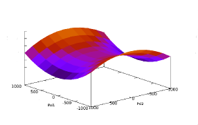
Figure 1. Anomalous interaction potential derived from the non-local transformation in [9].

Now, we can return to the formulation used in this work. Here we develop a mechanism in order to attach interaction potentials into the complex Bernard-Duncan model using the reality conditions.

The procedure is based specifically, i.e. on the real reduction, we consider all the possible interactions in the complex theory that are real quantities applying the reality conditions (3.14). The simplest examples are

(5.2) $$V^{1}=\int\!d^{3}x\frac{g_{1}}{4!(m_{1}^{2}-m_{2}^{2})^{2}}[m_{1}^{2}\phi-\pi_{\dot{\phi}}]^{4},$$

(5.3) $$V^{2}=\int\!d^{3}x\frac{g_{2}}{4!(m_{1}^{2}-m_{2}^{2})^{2}}[m_{2}^{2}\phi-\pi_{\dot{\phi}}]^{4}$$

and

(5.4) $$V^{3}=\int\!d^{3}x\frac{g_{3}}{4!(m_{1}^{2}-m_{2}^{2})^{2}}[m_{1}^{2}\phi-\pi_{\dot{\phi}}]^{2}[m_{2}^{2}\phi-\pi_{\dot{\phi}}]^{2}.$$

These expressions in terms of the fields $\psi_{1}$, $\psi_{2}$ including the reality conditions (3.14) are

(5.5) $$V^{1}\mid_{RC}=\int\!d^{3}x\frac{g_{1}}{4!}\psi_{2}^{4},\qquad V^{2}\mid_{RC}=\int\!d^{3}x\frac{g_{2}}{4!}\psi_{1}^{4},$$

$$V^{3}\mid_{RC}=\int\!d^{3}x\frac{g_{3}}{4!}\psi_{2}^{2}\psi_{1}^{2}$$

and we can join these potentials to obtain the effective potential

(5.6) $$V\mid_{RC}=m_{1}^{2}\psi_{1}^{2}+m_{2}^{2}\psi_{2}^{2}+V^{1}\mid_{RC}+V^{2}\mid_{RC}+V^{3}\mid_{RC},$$

with its graphic given by the figure 2.

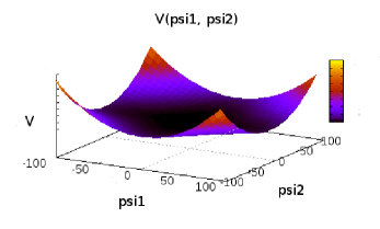
Figure 2. Potential $V\mid_{RC}$ that has a perturbative expansion.

This shows that we have achieved to obtain a potential with a minimum which we can apply a perturbative method.

In (3.18), the fields $\psi_{1}$ and $\psi_{2}$ obey free equations of motion. Then by means of this free description we can write the S-matrix.

The S-matrix elements are

(5.7) $$S_{fi}=_{out}<k^{\prime}_{1},k^{\prime}_{2},...|T\exp[-i\int_{-\infty}^{\infty}dt\ V^{k}\mid_{RC}(\psi_{1},\psi_{2})\mid_{cre}]|k_{1},k_{2},...>_{in}$$

with $k=1,2,3$. It is worth to mention that the reality conditions produce Hermitian fields $\psi$ then we wrote it in an usual way. So we can use (4.3) in order to do a perturbative expansion. From this description the Wick’s theorem can be shown and the time-order product is reduced into the normal ordered product as we usually do. However, we pay attention to irreducible diagrams $\frac{1}{i}\Sigma_{j}(p)$ with $j=1,2$ in order to describe self energy process. The propagator is

(5.8) $$G^{(2)}_{cj}(p)=\frac{i}{p^{2}-m_{Bj}^{2}-\Sigma_{j}(p)},$$

or

(5.9) $$[G^{(2)}_{cj}(p)]^{-1}=G_{0j}(p)^{-1}-\frac{1}{i}\Sigma_{j}(p).$$

It is important to consider the relationship between the physical mass and the complete propagator

(5.10) $$G^{(2)}_{cj}(p)=\frac{i}{p^{2}-m_{physj}^{2}}$$

and to consider

(5.11) $$m_{physj}^{2}=m_{Bj}^{2}+\Sigma_{j}(p).$$

Now, it is necessary to include a new definition in order to obtain the two points vertex function defined by

(5.12) $$G_{cj}^{(2)}(p)\Gamma_{j}(p)=i,$$

which is finally

(5.13) $$\Gamma_{j}(p)=p^{2}-m_{Bj}^{2}-\Sigma_{j}(p).$$

Using the above expression for each mass

(5.14) $$\Gamma_{2}(p)=p^{2}-m_{B2}^{2}-\Sigma_{2}(p),\qquad\Gamma_{1}(p)=p^{2}-m_{B1}^{2}-\Sigma_{1}(p),$$

we have obtained the two points vertex functions.

According to the Feynman rules, we fix the propagators by means of including self-interactions. For the propagator associated with $m_{B2}$, we obtain the figure 3.

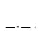
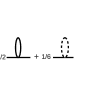
Figure 3. Two legs diagrams for the compleat propagator $G^{(2)}_{c2}(p)$ until order $\mathcal{O}(g^{3}_{1,3})$.

The analytic expression for $\Sigma_{2}(p)$ is

(5.15) $$\Sigma_{2}(p)=\frac{g_{1}}{2(2\pi)^{4}}\int\frac{d^{4}k_{E}}{k_{E}^{2}+m^{2}_{B2}}+\frac{g_{3}}{6(2\pi)^{4}}\int\frac{d^{4}k_{E}}{k_{E}^{2}+m^{2}_{B1}}$$

$$-\frac{g_{1}^{2}}{6(2\pi)^{8}}\int\frac{d^{4}p_{E1}d^{4}p_{E2}}{[(p_{E1}+p_{E2}+q_{E})^{2}+m_{B2}^{2}][p_{E1}^{2}+m_{B2}^{2}][p_{E2}^{2}+m^{2}_{B2}]}$$

$$-\frac{g_{3}^{2}}{18(2\pi)^{8}}\int\frac{d^{4}p_{E1}d^{4}p_{E2}}{[(p_{E1}+p_{E2}+q_{E})^{2}+m_{B1}^{2}][p_{E1}^{2}+m_{B1}^{2}][p_{E2}^{2}+m^{2}_{B2}]}$$

$$-\frac{g^{2}_{1}}{4(2\pi)^{8}}\int\frac{d^{4}k_{E1}d^{4}k_{E2}}{[k_{E1}^{2}+m_{B2}^{2}]^{2}[k_{E2}^{2}+m^{2}_{B2}]}-\frac{g_{2}g_{3}}{12(2\pi)^{8}}$$

$$\int\frac{d^{4}k_{E1}d^{4}k_{E2}}{[k_{E1}^{2}+m_{B1}^{2}]^{2}[k_{E2}^{2}+m^{2}_{B1}]}-\frac{g_{1}g_{3}}{12(2\pi)^{8}}\int\frac{d^{4}k_{E1}d^{4}k_{E2}}{[k_{E1}^{2}+m_{B2}^{2}]^{2}[k_{E2}^{2}+m^{2}_{B1}]}$$

$$-\frac{g_{3}^{2}}{36(2\pi)^{8}}\int\frac{d^{4}k_{E1}d^{4}k_{E2}}{[k_{E1}^{2}+m_{B1}^{2}]^{2}[k_{E2}^{2}+m_{B2}^{2}]}$$

where $q_{E}=-p_{E}$. For the propagator associated with $m_{B1}$ we obtain similar expressions and diagrams, but we have to interchange dashed lines to continuous lines and continuous lines to dashed lines in the figure 3.

The analytic expression for $\Sigma_{1}(p)$ can be obtain changing $g_{1}\rightarrow g_{2}$, $m_{B2}\rightarrow m_{B1}$ and $m_{B1}\rightarrow m_{B2}$.

In the above expression have been developed a Wick rotation, because it permit to separate the divergent part of integrals by means of dimensional regularization.

The regularized expression for (5.15) is

(5.16) $$\Sigma_{2}(p)\approx\frac{m^{2}_{2B}g_{1}}{2(4\pi)^{2}}[\frac{2}{\epsilon}+\Psi(2)+ln(\frac{4\pi\mu^{2}_{R}}{m^{2}_{2B}})]$$

$$+\frac{m^{2}_{1B}g_{3}}{6(4\pi)^{2}}[\frac{2}{\epsilon}+\Psi(2)+ln(\frac{4\pi\mu^{2}_{IR}}{m^{2}_{1B}})]+\frac{g_{1}^{2}}{6(4\pi)^{4}}\times$$

$$\left\{3m_{2B}^{2}[\frac{2}{\epsilon^{2}}+\frac{2}{\epsilon}(\frac{3}{2}+\Psi_{1}+log(\frac{4\pi\mu_{R}^{2}}{m_{2B}^{2}}))]+\frac{q^{2}}{2\epsilon}\right\}$$

$$+\frac{g_{3}^{2}m_{1B}^{2}}{18(4\pi)^{4}}\times[\frac{(4+\frac{2m_{2B}^{2}}{m_{1B}^{2}})}{\epsilon^{2}}+\frac{4}{\epsilon}(-\gamma+log(\frac{4\pi\mu_{RI}^{2}}{m_{1B}^{2}}))$$

$$+\frac{2m_{2B}^{2}}{m_{1B}^{2}\epsilon}[-\gamma+log(\frac{4\pi\mu_{RI}^{2}}{m_{2B}^{2}})]+\frac{2}{\epsilon}+\frac{m_{2B}^{2}}{m_{1B}^{2}\epsilon}+\frac{q^{2}}{2\epsilon m_{1B}^{2}}]$$

$$+\frac{g_{1}^{2}m_{2B}^{2}}{4(4\pi)^{4}}\times[\frac{4}{\epsilon^{2}}+\frac{2(\psi(1)+\psi(2))}{\epsilon}-\frac{4}{\epsilon}log(\frac{m_{2B}^{2}}{4\pi\mu_{R}^{2}})]$$

$$+\frac{g_{2}g_{3}m_{1B}^{2}}{12(4\pi)^{4}}[\frac{4}{\epsilon^{2}}+\frac{2(\psi(1)+\psi(2))}{\epsilon}-\frac{2}{\epsilon}log(\frac{m_{1B}^{2}}{4\pi\mu_{I}\mu_{RI}})]$$

$$+\frac{g_{3}g_{1}m_{1B}^{2}}{12(4\pi)^{4}}[\frac{4}{\epsilon^{2}}+\frac{2(\psi(1)+\psi(2))}{\epsilon}-\frac{2}{\epsilon}log(\frac{m_{2B}^{2}}{4\pi\mu_{R}\mu_{RI}})]$$

$$+\frac{g^{2}_{3}m_{2B}^{2}}{36(4\pi)^{4}}[\frac{4}{\epsilon^{2}}+\frac{2(\psi(1)+\psi(2))}{\epsilon}-\frac{2}{\epsilon}log(\frac{m_{1B}^{2}}{4\pi\mu_{RI}^{2}})]$$

with $\Psi(2)=1-\gamma$, $\Psi(z)=\frac{\Gamma^{\prime}(z)}{\Gamma(z)}$ and $\gamma$ being the Euler’s constant.

The physical masses are

(5.17) $$m_{2phy}^{2}=-\Gamma_{2}^{(2)}(0),\qquad m_{1phy}^{2}=-\Gamma_{1}^{(2)}(0)$$

and the relation between bare and renormalized masses is

(5.18) $$m_{2B}^{2}=[1-\frac{1}{\epsilon}(\frac{g_{1}}{(4\pi)^{2}}+\frac{g_{1}^{2}}{2(4\pi)^{4}}+\frac{g_{1}^{2}(\Psi(1)+\Psi(2))}{(4\pi)^{4}}$$

$$+\frac{g_{3}^{2}(\Psi(1)+\Psi(2))}{18(4\pi)^{4}})-(\frac{2g_{1}^{2}}{(4\pi)^{4}}-\frac{g_{3}^{2}}{9(4\pi)^{4}}+\frac{2g_{1}g_{2}}{(4\pi)^{4}})\frac{1}{\epsilon^{2}}]m_{2phy}^{2}$$

$$-[\frac{1}{\epsilon}(\frac{g_{3}}{(4\pi)^{2}}-\frac{8\gamma g_{3}^{2}}{9(4\pi)^{4}}+\frac{g_{2}g_{3}(\Psi(1)+\Psi(2))}{6(4\pi)^{4}}$$

$$+\frac{g_{1}g_{3}(\Psi(1)+\Psi(2))}{6(4\pi)^{4}})+(\frac{2g_{3}^{2}}{9(4\pi)^{4}}+\frac{4g_{1}g_{3}}{3(4\pi)^{4}}+\frac{4g_{2}g_{3}}{3(4\pi)^{4}})\frac{1}{\epsilon^{2}}]m^{2}_{1ph}$$

for $m^{2}_{1}$, we obtain

(5.19) $$m_{1B}^{2}=[1-\frac{1}{\epsilon}(\frac{g_{2}}{(4\pi)^{2}}+\frac{3g_{2}^{2}}{2(4\pi)^{4}}+\frac{2g_{2}^{2}(\Psi(1)+\Psi(2))}{(4\pi)^{4}}$$

$$+\frac{g_{3}^{2}(\Psi(1)+\Psi(2))}{18(4\pi)^{4}})-(\frac{g_{1}^{2}+2g_{2}^{2}}{(4\pi)^{4}}-\frac{2g_{3}^{2}}{9(4\pi)^{4}}+\frac{5g_{1}g_{2}}{4(4\pi)^{4}})\frac{1}{\epsilon^{2}}]m_{1phy}^{2}$$

$$-[\frac{1}{\epsilon}(\frac{g_{3}}{3(4\pi)^{2}}-\frac{4\gamma g_{3}^{2}}{9(4\pi)^{4}}+\frac{g_{1}g_{3}(\Psi(1)+\Psi(2))}{6(4\pi)^{4}}$$

$$+\frac{g_{2}g_{3}(\Psi(1)+\Psi(2))}{6(4\pi)^{4}})+(\frac{2g_{3}^{2}}{9(4\pi)^{4}}+\frac{2g_{1}g_{3}}{3(4\pi)^{4}}+\frac{2g_{2}g_{3}}{3(4\pi)^{4}})\frac{1}{\epsilon^{2}}]m^{2}_{2ph}.$$

We now apply a similar treatment to $\Gamma^{(4)}$ in order to renormalize the coupling constant $g_{j}$. We can consider the new momenta $k_{E}=p_{4E}-p_{2E}=p_{1E}-p_{3E}$, $k^{\prime}_{E}=p_{3E}-p_{2E}$ and $k^{\prime\prime}_{E}=p_{1E}+p_{2E}=p_{3E}+p_{4E}$ in order to calculate the four-points function to take into account the amputated diagrams that are in the figure 4. The analytic expression of the figure 4 is

(5.20) $$\Gamma_{1}^{(4)}(p_{1E},p_{2E},p_{3E},p_{4E})=-ig_{1}$$

$$+\frac{ig_{1}^{2}}{2(2\pi)^{4}}\int\frac{d^{4}q_{E}}{[(q_{E}+k_{E})^{2}+m_{2B}^{2}][q_{E}^{2}+m_{2B}^{2}]}$$

$$+\frac{ig_{1}^{2}}{2(2\pi)^{4}}\int\frac{d^{4}q_{E}}{[(q_{E}+k^{\prime}_{E})^{2}+m_{2B}^{2}][q_{E}^{2}+m_{2B}^{2}]}$$

$$+\frac{ig_{1}^{2}}{2(2\pi)^{4}}\int\frac{d^{4}q_{E}}{[(q_{E}+k^{\prime\prime}_{E})^{2}+m_{2B}^{2}][q_{E}^{2}+m_{2B}^{2}]}$$

$$+\frac{ig_{3}^{2}}{18(2\pi)^{4}}\int\frac{d^{4}q_{E}}{[(q_{E}+k_{E})^{2}+m_{1B}^{2}][q_{E}^{2}+m_{1B}^{2}]}$$

$$+\frac{ig_{3}^{2}}{18(2\pi)^{4}}\int\frac{d^{4}q_{E}}{[(q_{E}+k^{\prime\prime}_{E})^{2}+m_{1B}^{2}][q_{E}^{2}+m_{1B}^{2}]}$$

$$+\frac{ig_{3}^{2}}{18(2\pi)^{4}}\int\frac{d^{4}q_{E}}{[(q_{E}+k^{\prime}_{E})^{2}+m_{1B}^{2}][q_{E}^{2}+m_{1B}^{2}]}.$$

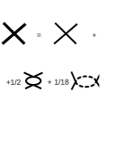
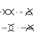
Figure 4. One-loop four-points function for $g_{1}$, $g_{3}$.

Putting

(5.21) $$F(s,m,\mu)\equiv\int_{0}^{1}\!dx\ \ln(\frac{sx(1-x)+m^{2}}{4\pi\mu^{2}})$$

the regularized expression for (5.20) is

(5.22) $$\Gamma_{1}^{(4)}(p_{1E},p_{2E},p_{3E},p_{4E})\approx-ig_{B1}\mu^{\epsilon}_{R}+\frac{3ig_{B1}^{2}\mu_{R}^{\epsilon}}{16\pi^{2}\epsilon}$$

$$+\frac{ig_{B3}^{2}\mu_{RI}^{\epsilon}}{48\pi^{2}\epsilon}-\frac{ig_{B1}^{2}\mu_{R}^{\epsilon}}{32\pi^{2}}[3\gamma+F(k_{E}^{2},m_{2},\mu_{R})$$

$$+F(k_{E}^{{}^{\prime}2},m_{2},\mu_{R})+F(k_{E}^{{}^{\prime\prime}2},m_{2},\mu_{R})]$$

$$-\frac{ig_{B3}^{2}\mu_{RI}^{\epsilon}}{288\pi^{2}}[3\gamma+F(k_{E}^{2},m_{1},\mu_{RI})$$

$$+F(k_{E}^{{}^{\prime}2},m_{1},\mu_{RI})+F(k_{E}^{{}^{\prime\prime}2},m_{1},\mu_{RI})].$$

As in $\Gamma^{(2)}_{1}$, we obtain similar expressions to $\Gamma^{(4)}_{2}$ interchanging dashed lines to continuous lines and continuous lines to dashed lines. For the analytic expression it is changed $g_{1}\rightarrow g_{2}$, $m_{1}\rightarrow m_{2}$ and $m_{2}\rightarrow m_{1}$.

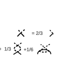
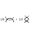
Figure 5. One-loop four-points function with different external legs for $g_{1}$, $g_{2}$ and $g_{3}$.

with $j=1,2,3$ and $k=1,2,3,4$. The corresponding renormalization is

(5.23) $$g_{B1}\approx g_{1phy}\mu^{-\epsilon}_{R}+\frac{3g_{1phy}^{2}\mu_{R}^{-2\epsilon}}{16\pi^{2}\epsilon}$$

$$+\frac{9g_{3phy}^{2}\mu_{RI}^{-\epsilon}\mu_{R}^{-\epsilon}}{192\pi^{2}\epsilon}-\frac{g_{1phy}^{2}\mu_{R}^{-\epsilon}}{32\pi^{2}}[3\gamma+F(0,m_{2phy},\mu_{R})$$

$$+F(0,m_{2phy},\mu_{R})+F(0,m_{2phy},\mu_{R})]$$

$$-\frac{9g_{3phy}^{2}\mu_{RI}^{-\epsilon}}{1152\pi^{2}}[3\gamma+F(0,m_{1phy},\mu_{RI})$$

$$+F(0,m_{1phy},\mu_{RI})+F(0,m_{1phy},\mu_{RI})]$$

and for the other coupling constant, we have

(5.24) $$g_{B2}\approx g_{2phy}\mu^{-\epsilon}_{I}+\frac{3g_{1phy}^{2}\mu_{I}^{-2\epsilon}}{16\pi^{2}\epsilon}$$

$$+\frac{9g_{3phy}^{2}\mu_{RI}^{-\epsilon}\mu_{I}^{-\epsilon}}{192\pi^{2}\epsilon}-\frac{g_{1phy}^{2}\mu_{I}^{-\epsilon}}{32\pi^{2}}[3\gamma+F(0,m_{1phy},\mu_{I})$$

$$+F(0,m_{1phy},\mu_{I})+F(0,m_{1phy},\mu_{I})]$$

$$-\frac{9g_{3phy}^{2}\mu_{RI}^{-\epsilon}}{1152\pi^{2}}[3\gamma+F(0,m_{2phy},\mu_{RI})$$

$$+F(0,m_{2phy},\mu_{RI})+F(0,m_{2phy},\mu_{RI})].$$

Because we have three vertexes the regularization for the coupling constant $g_{3}$, given by diagrams in figure 5, is

(5.25) $$g_{3}\approx\frac{3g_{3phy}\mu^{-\epsilon}_{RI}}{2}$$

$$+\frac{9g^{2}_{3phy}\mu_{RI}^{-2\epsilon}}{64\pi^{2}\epsilon}+\frac{3g_{3phy}\mu_{RI}^{-\epsilon}(\mu_{R}^{-\epsilon}g_{1phy}+\mu_{I}^{-\epsilon}g_{2phy})}{2\pi^{2}\epsilon}-\frac{3g^{2}_{3phy}\mu_{RI}^{-\epsilon}}{192\pi^{2}}[2\gamma$$

$$+\int_{0}^{1}\!\ln(\frac{m_{2phy}^{2}+(m_{1phy}^{2}-m_{2phy}^{2})x}{4\pi\mu_{RI}^{2}})dx$$

$$+\int_{0}^{1}\!\ln(\frac{m_{2phy}^{2}+(m_{1phy}^{2}-m_{2phy}^{2})x}{4\pi\mu_{RI}^{2}})dx]$$

$$-\frac{3g_{3phy}}{96\pi^{2}}[(\mu_{R}^{-\epsilon}g_{1phy}+\mu_{I}^{-\epsilon}g_{2phy})\gamma+\mu_{R}^{-\epsilon}g_{1phy}F(0,m_{2},\mu_{R})$$

$$+\mu_{I}^{-\epsilon}g_{2phy}F(0,m_{1},\mu_{I})].$$

The above method works without problems, but we have eliminated the Hermiticity condition for the higher order derivative field. It allowed us to include interaction potentials in the higher order derivative theory that were mapped to real interaction potentials by means of the reality conditions, see figure 2. The mapping here described results in a renormalizable theory without inherent pathologies from the higher order derivative theories [9] as it was shown in the figure 1.

6. Conclusions

The higher order derivative theories are an alternative description of the nature that can be encoded to the usual first order mechanics. The above is seen by means of the existence of a canonical transformation between the real Bernard-Duncan Hamiltonian density and the Hamiltonian density of two real Klein-Gordon fields with opposite sign [6]. In the classical context the equations of motion are equivalent and also to the quantum level but in this case the system suffers irremediable inconsistencies once we include interactions in the system. In this case the effective potential is instable, see figure 1.

If we look at a canonical transformation from the Bernard-Duncan Hamiltonian Density to Hamiltonian density of two Klein-Gordon fields with positive sign, it is necessary to introduce a complex canonical transformation [12] resulting in a complex extension of the Bernard-Duncan Hamiltonian. Fundamental to this formulation is to show that a restricted complex description is equivalent to the usual classic description. This is achieved by showing that the equations of motion resulting from both formulations are equivalent.

Since, our starting point is now a complex higher order derivative theory to quantize the system we disregard the Hermiticity axiom. The alternative to this condition is to use the so called reality conditions [13]. Using these conditions we map the complex higher order derivative theory to a real first order theory in Section 4. These conditions are really constraints to the complex theory and reduce the degrees of freedom and the most important are consistent with a class of interactions. In spite of the higher order derivative field isn’t Hermitian, if the reality conditions are considered, the resulting fields and the Hamiltonian density will be Hermitian quantities. The initial description isn’t Hermitian, but the reduction imposed by the reality condition is Hermitian.

The way to attach the reality conditions in this work was through annihilation and creation operators instead of considering the Hermiticity conditions. The complex extension give us a greater flexibility and in this way it is still possible to obtain an Hermitian theory (4.17).

The reality conditions also allow us to establish the interaction potentials (5.2)-(5.4) that generate real interaction potentials (5.5) imposing the conditions (4.1) and resulting a total potential that has a minimum critical point. In consequence, it makes possible a perturbative expansion as in the figure 2 and a regularizable and renormalizable theory.

It is instructive here to summarize this work. According to section 3, we introduced the complex Bernard-Duncan model using the action and it was established the complex Bernard-Duncan Hamiltonian density. Using this complex density, we set a mapping from this one to the real Hamiltonian density of two Klein-Gordon fields [12]. By means of this mapping, we obtained the reality conditions that, according to section 4, was applied by means of annihilation and creation operators and they replaced the Hermiticity conditions resulting the Hamiltonian density of two real Klein-Gordon fields. This Hamiltonian density, according to section 5, allow us to include interaction potentials in a regularizable and renormalizable way.

References

[1] Ostrogradski, M.V.: Mémoires sur les équations differentielles relatives au problème des
isopérimetrètres. Mem. Acad. St. Petersburg 6, 385-517 (1850).
[2] Smilga, A.: Comments on the Dynamics of the Pais-Uhlenbeck Oscillator. Sigma 5, 017 (2009).
[3] Mostafazadeh, A.: Imaginary-Scaling versus Indefinite-Metric Quantization
of the Pais-Uhlenbeck Oscillator. Phys. Rev.D84, 105018 (2011).
[4]Stelle, K. S.: Classical Gravity with Higher Derivatives. Phys. General Relativity and Gravitation,
9, 353-371 (1978).
[5] Schaposnik, F.A.: Chiral Symmetry in The Path Integral
Approach. CNPq/CBPF, 15-21 (1986).
[6] Pais, A., Uhlenbeck, G.E.: On Field with Non- Localized Action. Phys. Rev. 79, 145-165 (1950).
[7] Eliezer,D., Woodard, R.: The Problem of Nonlocality In String Theory. Nucl. Phys. B325, 389 (1989).
[8] Bernard,C., Duncan, A.: Lorentz covariance and Matthews’s theorem for derivative-coupled field theories.
Phys. Rev.D11,848-859 (1975).
[9] Hawking, S.W., Hertog,T.: Living with ghosts. Phys. Rev.
D. 65,389 (2002).
[10] Antoniadis, I., Dudas, E.,Ghilencea, D.M.: Living with ghosts and
their radiative corrections. Nucl. Phys. B767,29-53 (2007).
[11] Bender,C.M., Mannheim, P.D.: Exactly solvable -symmetric
Hamiltonian having no Hermitian counterpart. Phys. Rev. D78, 0255022 (2008).
[12] Dector,A., Morales- Técotl,H. A., Urrutia,L.F., Vergara,J.D.:
An Alternative Canonical Approach to the Ghost Problem in a complexified Extension of the Pais-Uhlenbeck Oscillator.
SIGMA 5, 053 (2009).
[13] Ashtekar, A.: Lectures on Non-perturbative Canonical Gravity. World Scientific, Singapore (1991).
[14] Margalli, C. and Vergara, J. D., in
preparation.