Phase segregation of superconductivity and ferromagnetism at LaAlO₃/SrTiO₃ interface

Abstract

The highly conductive two-dimensional electron gas formed at the interface between insulating SrTiO₃ and LaAlO₃ shows low-temperature superconductivity coexisting with inhomogeneous ferromagnetism. The Rashba spin-orbit interaction with in-plane Zeeman field of the system favors $p_{x}\pm ip_{y}$-wave superconductivity at finite momentum. Owing to the intrinsic disorder at the interface, the role of spatial inhomogeneity on the superconducting and ferromagnetic states becomes important. We find that for strong disorder, the system breaks up into mutually excluded regions of superconductivity and ferromagnetism. This inhomogeneity-driven electronic phase separation accounts for the unusual coexistence of superconductivity and ferromagnetism observed at the interface.

I Introduction

The physics underlying the interface sandwiched between insulating oxides SrTiO₃ and LaAlO₃ has generated tremendous excitement in the last few years after the discovery of a high mobility two dimensional electron gas (2DEG) at the interface Ohtomo2004 . In 2007, Reyren, et al. Reyren31082007 found that the system is superconducting below 200 mK. The other intriguing phenomena the 2DEG exhibits are electric field induced metal-insulator transition Cen2008 ; Caviglia2008 ; lu:172103 and superconductor-insulator transition PhysRevLett.103.226802 . In particular, there are strong evidences that the superconductivity coexists with a finite magnetic moment (0.3-0.4 $\mu_{B}$ per interface unit cell) PhysRevLett.107.056802 . Torque magnetometry and transport measurements report an in-plane magnetic ordering from well below the superconducting transition to 200 K Li2011 . Scanning squid data reveals that, the sample contains sub-micrometer patches of ferromagnetic domain within a non-uniform background of weak diamagnetic superconducting susceptibility Bert2011 .

The highly unusual coexistence of superconductivity and ferromagnetism has spawned several theoretical efforts to unravel the nature of states at the interface. As proposed by Pavlenko, et al. PhysRevB.85.020407 , magnetism may not be an intrinsic property of the 2DEG, but is a result of the spin splitting of the populated electronic states induced by Oxygen vacancies in the SrTiO₃ or LaAlO₃ layer. The metallic behavior of the interface results from the 2D electron liquid produced by the electronic reconstruction. The metallic state is related to a superconducting state below 200 mK, occurring in regions of vanishing Oxygen vacancies. Michaeli, et al. PhysRevLett.108.117003 argued that due to strong spin-orbit interaction superconductivity and ferromagnetism can coexist via Fulde-Ferrell-Larkin-Ovchinnikov (FFLO) type pairing at finite momentum; the FFLO state being quite sensitive to disorder while possibly even stabilized by strong disorder.

According to Fidkowski, et al. PhysRevB.87.014436 , droplets of superconductivity are formed in the bulk insulating SrTiO₃ due to some imperfections in the lattice. In presence of LaAlO₃, the mobile electrons in the 2DEG mediate a coupling between the droplets which percolate and grow until a long-range superconducting order forms. Another recent suggestion 2013arXiv1304.2970C is multi-band superconductivity resulting from percolation of filamentary structures of superconducting puddles. Recently, Randeria, et al. Banerjee2013 proposed that the ground state magnetization is a long-wavelength spiral aligning to a weak ferromagnetism in the presence of applied magnetic field. Several studies have provided hints, but not yet conclusive support for the existence of superconductivity and ferromagnetism and their coexistence.

It is now well-understood that the metallic conduction at the interface is mainly due to two reasons: the Oxygen vacancies at the interface PhysRevX.3.021010 ; PhysRevB.86.064431 ; Schlom2011 and an intrinsic electronic transfer mechanism known as polar catastrophe in which half an electronic charge is transferred to the interface  Nakagawa2006 ; PhysRevB.80.075110 . The electrons at the interface, which is TiO₂ terminated, occupy the 3d $t_{2g}$ orbital of Ti atoms. Michaeli, et al. PhysRevLett.108.117003 pointed out that there are three different bands, uniformly distributed at the interface, responsible for superconductivity and ferromagnetism. The $d_{xy}$ band is wider than the $d_{xz}$, $d_{yz}$ bands and is relatively lower in energy at the $\Gamma$ point. It is therefore likely that the electrons in this band get localized at the interface sites due to Coulomb correlation and eventually form localized moments. A ferromagnetic local exchange interaction between the conduction band electrons and the local moments will thereafter lead to an effective in-plane Zeeman field. The Zener kinetic exchange may then order local moments as well. Very recently, spectroscopic studies provided direct evidence for in-plane ferromagnetism of electrons with $d_{xy}$ character Lee2013 . Another important feature of the system is the large Rashba coupling which originates from the broken inversion symmetry in the two-dimensional interface plane.

It is more or less evident that inhomogeneities at the interface, in the form of Oxygen vacancies and intrinsic disorder, are an inseparable part of the interface. It is therefore likely that they have a profound effect on the long range orders and their coexistence at the interface. In the following analysis, we use inhomogeneous Bogoliubov-de Gennes (BdG) theory to study the effects of non-magnetic disorder on superconductivity and magnetism at the interface in presence of a strong Rashba coupling. Our calculations show that due to large disorder, the system forms superconducting islands. At the regions where superconductivity is destroyed by disorder, electrons order ferromagnetically along the plane due to the in-plane field forming ferromagnetic domains. This disorder-driven electronic phase separation enables superconductivity and ferromagnetism to coexist in the same sample in electronically phase-separated regions. Electronic phase separation as a mechanism for coexistence of various long-range orders has been established in manganites in the last decade PhysRevLett.80.845 ; Dagotto20011 . Its role in the interfaces has also been posited by some experimental groups and a theoretical analysis in the present context is therefore eminently topical.

The rest of the paper is organized as follows. In the next section, we describe our model for a Rashba spin-orbit-coupled superconductor in presence of an in-plane Zeeman field. In section III, starting with the standard inhomogeneous BdG mean-field formalism, we present and analyze the effects of spatial inhomogeneity on superconductivity and ferromagnetism and their possible coexistence at the interface. In addition, we extend our analysis to finite temperatures and study the coexistence. Sections IV and  V are for discussions of results and concluding remarks.

II Model

Electrons at the interface occupy the $t_{2g}$ bands of Ti atom and therefore these bands are thought to be responsible for superconductivity and ferromagnetism in the system. The electrons occupying $d_{xy}$ band, which is much wider than $d_{xz}$ or $d_{yz}$ bands and is lower in energy at the $\Gamma$ point, are localized due primarily to the electron-electron correlation at the interface. The local moments interact via exchange interaction with the electrons in conduction band (claimed to be slightly below the terminating TiO₂ layer in the SrTiO₃ side PhysRevLett.108.117003 ) leading to an in-plane Zeeman field. Superconductivity originates from a short-range electron-electron attractive interaction of strength $U$ (possibly retarded by the phonon energies). The following Hamiltonian describes a Rashba spin-orbit coupled superconductor in an in-plane Zeeman field.

$$\begin{split}&{\cal H}={\cal H}_{0}+{\cal H}_{ex}+{\cal H}_{so}+{\cal H}_{sc},\\ &{\cal H}_{0}=\sum_{k,\sigma}\epsilon_{k}c_{k\sigma}^{\dagger}c_{k\sigma}\\ &{\cal H}_{ex}=-\sum_{k,\sigma,\sigma^{\prime}}(\bm{H}\cdot\bm{\sigma})_{\sigma,\sigma^{\prime}}c_{k\sigma}^{\dagger}c_{k\sigma^{\prime}}\\ &{\cal H}_{so}=\alpha\sum_{k,\sigma,\sigma^{\prime}}(\bm{R}(\bm{k})\cdot\bm{\sigma})_{\sigma,\sigma^{\prime}}c_{k\sigma}^{\dagger}c_{k\sigma^{\prime}}\\ &{\cal H}_{sc}=-U\sum_{k,k^{\prime}}c_{k\uparrow}^{\dagger}c_{-k\downarrow}^{\dagger}c_{k^{\prime}\downarrow}c_{-k^{\prime}\uparrow}\end{split}$$ (1)

where, $\epsilon_{k}=-2t(\cos k_{x}+\cos k_{y})-\mu$ with hopping amplitude $t$ in a square lattice and chemical potential $\mu$. The in-plane Zeeman field is given by $H=(H_{x},H_{y},0)$ and the Rashba coupling is $R({\bm{k}})=(\sin k_{y},-\sin k_{x})$, $\bm{\sigma}$ being the Pauli matrices. The Rashba spin-orbit interaction creates helical bands in which the electron spins are aligned with respect to the direction of propagation as shown in Fig. 1(a). The energy bands, created by the Rashba SOC with in-plane Zeeman field, are given by

$$\epsilon_{\pm}(\mathbf{k})=\epsilon_{k}\pm|\alpha\bm{R}(\bm{k})-\bm{H}|$$ (2)

and the corresponding eigenstates $c_{k,\pm}$ are obtained by the following transformation

$$\begin{split}\begin{pmatrix}\begin{array}[]{c}c_{k\uparrow}\\ c_{k\downarrow}\end{array}\end{pmatrix}&=\frac{1}{\sqrt{2}}\begin{pmatrix}\begin{array}[]{cc}1&1\\ e^{i\phi_{k}}&-e^{i\phi_{k}}\end{array}\end{pmatrix}\begin{pmatrix}\begin{array}[]{c}c_{k,+}\\ c_{k,-}\end{array}\end{pmatrix}\end{split}$$ (3)

where $\phi_{k}=\tan^{-1}(\frac{-\sin k_{x}-H_{y}}{\sin k_{y}-H_{x}})$.

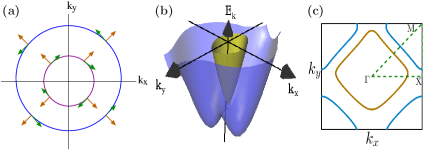
Figure 1: (Color online) (a) Two-sheeted Fermi surface of the Rashba-splited bands showing the helical alignment of the spins (green) and corresponding momentum (orange). The (b) resultant bands and (c) asymmetric Fermi surface created by Rashba spin-orbit interaction with Zeeman field along $\hat{x}$ direction.

In the chiral basis $[c_{k,+},c_{k,-}]$, ${\cal H}_{0}+{\cal H}_{ex}+{\cal H}_{so}$ is diagonal and ${\cal H}_{sc}$ has the pairing symmetry of $p_{x}\pm ip_{y}$ superconductivity:

$${\cal H}_{sc}=\sum_{k}\Delta(e^{-i\phi_{k}}c_{k,+}^{\dagger}c_{-k,+}^{\dagger}+e^{i\phi_{k}}c_{k,-}^{\dagger}c_{-k,-}^{\dagger}+h.c.)$$ (4)

with $\Delta$ as the pairing amplitude. The Zeeman field in the in-plane direction shifts the Fermi surface from the center of the Brillouin zone, as shown in Fig. 1(b) and (c), and therefore removes the degeneracy of a pair of electrons on the Fermi surface with opposite wave vectors ${\bm{k}}$ and $-{\bm{k}}$. Hence for pairing of electrons with same energy, it turns out to be energetically favorable to have a finite center of mass momentum (proportional to the in-plane field PhysRevB.81.184502 ) of the pair.

In a clean system, the field due to moments at the interface is fairly strong and may even be larger than superconducting critical field PhysRevLett.108.117003 . In that case the system becomes magntically ordered. On the other hand, if the field is not strong enough, supreconductivity may dominate in a homogeneous system. However, disorder has a significant effect on the superconducting state (particularly for non-s-wave cases) and in turn lead to islands of non-superconducting regions. Phase segregation in real space is a likely outcome in such inhomogeneous situations and superconductivity and ferromagnetism coexist. The following Bogoliubov-de Gennes analysis explores the role of disorder on the superconductivity in such a system.

III Role of spatial Inhomogeneity

The interplay between superconductivity and disorder has been a central issue of many recent investigations on superconductivity PhysRevB.65.014501 ; dubinature2007 ; Chatterjee2008582 . With increasing disorder, there exists a phase transition from superconductor to insulator in two-dimensional thin films PhysRevLett.65.923 . The Rashba spin-orbit interaction induces chiral $p_{x}\pm ip_{y}$-wave superconductivity where Anderson’s theorem, unlike in conventional s-wave superconductors, is not applicable. Hence, it is interesting to study the effect of non-magnetic disorder on a two-dimensional system with both ferromagnetism and unconventional superconductivity, especially when there is broken mirror symmetry.

We consider the following BdG Hamiltonian for a Rashba coupled superconductor on a square lattice with an effective Zeeman field along the $\hat{x}$ direction (without any loss of generality only the $x$-component of the field is considered for simplicity),

$$\begin{split}{\cal H}_{BdG}&=-t\sum_{<ij>,\sigma}(c_{i\sigma}^{\dagger}c_{j\sigma}+h.c.)-\sum_{i,\sigma}(\mu-V{{}_{i}})c_{i\sigma}^{\dagger}c_{i\sigma}\\ &-H_{x}\sum_{i,\sigma,\sigma^{\prime}}(\sigma_{x})_{\sigma\sigma^{\prime}}c_{i\sigma}^{\dagger}c_{i\sigma^{\prime}}+\sum_{i}\Delta(r_{i})(c_{i\uparrow}^{\dagger}c_{i\downarrow}^{\dagger}+h.c.)\\ &-i\frac{\alpha}{2}\sum_{<ij>,\sigma,\sigma^{\prime}}c_{i\sigma}^{\dagger}(\bm{\sigma}_{\sigma\sigma^{\prime}}\times\bm{d}_{ij})_{z}c_{j\sigma^{\prime}}\end{split}$$ (5)

where $V_{i}$ is the random disorder in the local chemical potential, taken to be uniformly distributed between [-W,W]. ${\cal H}_{BdG}$ is diagonalized via a spin-generalized Bogoliubov-Valatin transformation $\hat{c}_{i\sigma}(r_{i})=\sum_{i,\sigma^{\prime}}u_{n\sigma\sigma^{\prime}}(r_{i})\hat{\gamma}_{n\sigma^{\prime}}+v_{n\sigma\sigma^{\prime}}^{*}(r_{i})\hat{\gamma}^{\dagger}_{n\sigma^{\prime}}$. This gives the following equation for the local order parameter $\Delta(r_{i})=-U<c_{i\uparrow}c_{i\downarrow}>$ in terms of the Bogoliubov amplitudes $u_{n\sigma}(r_{i})$ and $v_{n\sigma}(r_{i})$:

$$\begin{split}\Delta(r_{i})=&-U\sum_{n}[u_{n\uparrow}(r_{i})v^{*}_{n\downarrow}(r_{i})(1-f(E_{n}))\\ &+u_{n\downarrow}(r_{i})v^{*}_{n\uparrow}(r_{i})f(E_{n})]\end{split}$$ (6)

where $f(x)=1/(1+e^{x/{k_{B}T}})$ is the Fermi function at temperature $T$. The in-plane magnetization density with exchange field along $\hat{x}$ direction is obtained via

$$\begin{split}m(r_{i})&=<c_{i\uparrow}^{\dagger}c_{i\downarrow}+c_{i\downarrow}^{\dagger}c_{i\uparrow}>\\ &=\sum_{n,\sigma}u_{n\sigma}^{*}u_{n\sigma^{\prime}}f(E_{n})+v_{n\sigma}u_{n\sigma^{\prime}}^{*}(1-f(E_{n}))\end{split}$$ (7)

The orbital contribution to the magnetic moment is expected to be fairly small in the inhomogeneous, phase segregated situation with short superconducting mean-free path ($\xi$). In chiral superconductors, even for homogeneous condensates, this is a hotly debated issue and values of orbital moment range from $\hbar$ per pair to $k_{F}\xi$ or even $(k_{F}\xi)^{2}$ (i.e., corresponding moment of order $\mu_{B}$ or 10${}^{-6}\mu_{B}$; for recent results and comments on this, see Ref. 1367-2630-11-5-055063 ; JPSJ.65.664 ; Stone20082 ; PhysRevB.74.024408 ). Clearly, in an inhomogeneous situation such as the one obtains in the interface (with an intrinsically short $\xi$), the total effect coming from the magnetic domains would be much reduced. The experimental indicators certainly do not subscribe to a large contribution to the angular momentum, though careful experiments like Kerr rotation, X-ray circular dichroism, $\mu$SR and resonant Raman scattering are needed to resolve this. We have, therefore, ignored this in the foregoing and restricted ourselves to the spin contribution only.

The quasi-particle amplitudes $u_{n\sigma}(r_{i})$ and $v_{n\sigma}(r_{i})$ are determined by solving the following BdG equations:

$$\begin{split}{\cal H}_{BdG}\phi_{n}(r_{i})=\epsilon_{n}\phi_{n}(r_{i})\end{split}$$ (8)

where $\phi_{n}=[u_{n\uparrow}(r_{i}),u_{n\downarrow}(r_{i}),v_{n\uparrow}(r_{i}),v_{n\downarrow}(r_{i})]$.

In what follows, Eq.(6) and Eq.(8) are solved self-consistently on a finite, large two dimensional square lattice with periodic boundary conditions and finally the mean values are calculated using $\Delta=\frac{1}{N}\sum_{i}\Delta_{s}(r_{i})$ and $m=\frac{1}{N}\sum_{i}m(r_{i})$, over several realizations of the disorder. N is the total number of sites. The results presented here are obtained with $31\times 31$ lattice sites, which is large enough to obtain a quantitatively satisfactory description. We work in grand canonical ensemble with $t=1$ and $U=1$ (consistent with previous work PhysRevB.65.014501 ; PhysRevLett.81.3940 ) and unless specified, the density of electrons is kept at half-filling. The case of filling away from half is discussed later. We first discuss our results at $T=0$ and later extend to finite temperatures.

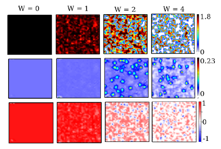
Figure 2: (Color online) The spatial distribution of the local pairing amplitude $|\Delta(r_{i})|$ (top row) and magnetization (middle row). The columns are for disorder strength $W=0$, $W=1$, $W=2$ and $W=4$ (from left to right). The lowest row shows the coexistence in combined plots of magnetization and local pairing amplitude; red and blue represent regions of superconductivity and ferromagnetism. The parameters used are $H_{x}=0.5$ and $\alpha=0.8$.

The inhomogeneous BdG method is useful to study the spatial variations of the pairing amplitude. In the large disorder regime, the microscopic details turn out to be very important leading to new unanticipated results. Fig. 2 shows the spatial distribution of the local pairing amplitude $|\Delta(r_{i})|$ for different disorder strengths. The top and middle row show the development of superconductivity and magnetism separately while the bottom one reveals the full picture of coexistence. In the homogenous system ($W=0$), superconductivity is uniform at the interface plane and the magnetic response is very weak. However, in the highly inhomogeneous case ($W\geq 2$), the disorder abets in breaking the uniform suprconductivity into islands separated by non-superconducting regions. It is quite straightforward to understand the underlying physical situation within the BdG formalism. The regions where $|\mu-V_{i}|$ is small, superconductivity sets in easily while the regions of large number fluctuations, having large $|\mu-V_{i}|$, militate against it. Robust ferromagnetic puddles are formed at the regions where superconductivity is degraded by disorder. Thus disorder helps the two competing phases to coexist by keeping them spatially seperated.

III.0.1 Distribution of pairing gap and magnetization

A great deal of information about the nucleation of the pairing on the microscopic scale can be extracted from the data plotted in Fig. 2. In Fig. 3(a), we plot the distribution of the local pairing amplitude $|\Delta(r_{i})|$ for a number of disorder strengths.

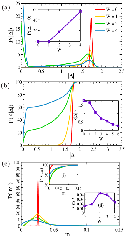
Figure 3: (Color online) (a) Probability distribution of local pairing amplitudes. Inset shows the variation of the probability at zero gap with disorder strength. (b) The curves show the probability P($<\Delta$) that the gaps are less than a given $\Delta$ for different disorder strength. Inset is $<|\Delta|>$ as a function of disorder strength. (c) The probability distribution of local magnetization. Inset (i) is P($<m$) as a function of $m$ and inset (ii) is the variation of average magnetization with disorder. The parameters used are $H_{x}=0.5$, $\alpha=0.8$ at $W=4$.

In the homogeneous system ($W=0$), there is a pronounced peak near $|\Delta_{0}|$, the mean-field value at $T=0$. As the disorder increases, the peak at $|\Delta_{0}|$ decreases, weight is gradually transferred to lower gap values and the probability for zero gap increases (shown in the inset of Fig. 3(a)), indicating the formation of non-superconducting regions. It is interesting to note that even for low disorder strength, regions with zero gap appear and long range superconducting order is severely affected as expected for a $p_{x}\pm ip_{y}$ superconductivity (in contrast with the s-wave case where the effect is indeed weaker PhysRevB.65.014501 ). From Fig. 2, we extract the probability P($<|\Delta|$) that the gap value is less than a given $|\Delta|$, as plotted in Fig. 3(b). This clearly demonstrates how the propensity towards formation of low-gap (and eventually gapless) regions increases rapidly with increasing disorder. The inset of Fig. 3(b) shows that the mean pairing amplitude $<|\Delta|>$ decreases strongly with increasing disorder. However, it never vanishes, as pointed out by Avishai, et al. dubinature2007 ; even in the strong disorder limits there are always few superconducting regions with finite gaps.

Disorder has significant effects on the resulting ferromagnetic landscape described by the probability distribution of local magnetization in Fig. 3(c). The peaks correspond to weak ferromagnetic background, which gradually shift towards zero as disorder increases. The tail at higher magnetizations, for $W\geq 2$ reflects the formation of ferromagnetic puddles at higher disorder strength. However, for very strong disorder, the ferromagnetic domains are also destroyed, reflected in the nature of the variation of average magnetization (inset (ii) of Fig. 3(c)). The competition between superconductivity and ferromagnetism is borne out from a comparison of the distributions P($<|\Delta|$) and P($<m$) for pairing amplitude and local magnetization respectively. With higher disorder, the probability P$(|\Delta|)$ of gapped regions decreases (Fig. 3(b)), while the regions of ferromagnetic domains increase (inset (i) of Fig. 3(c)). Thus the formation of robust ferromagnetism tracks the destruction of superconducting regions. Such a correlation is crucial for the observed formation of microscopically phase separated regions of ferromagnetism and superconductivity at the interface Wang2011 .

III.0.2 Correlation functions

To get a better understanding of the nature of superconducting regions or the ferromagnetic domains and the range of their order, it is useful to study the disorder-averaged correlation functions $D_{m}(|r_{i}-r_{j}|)=<m(r_{i})m(r_{j})>$ and $D_{sc}(|r_{i}-r_{j}|)=<|\Delta|(r_{i})|\Delta|(r_{j})>$.

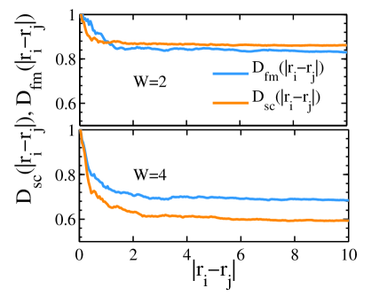
Figure 4: (Color online) Plots of the correlation functions ${D_{fm}(|r_{i}-r_{j}|)}$ and ${D_{sc}(|r_{i}-r_{j}|)}$ (see text) for local magnetizations and superconducting pair-amplitudes respectively as a function of the separation $|r_{i}-r_{j}|$. All the plots are normalized to unity at zero-separation. The parameters used are $H_{x}=0.5$, $\alpha=0.8$ at $T=0$.

As depicted in Fig. 4, both the correlation functions ${D_{sc}(|r_{i}-r_{j}|)}$ and ${D_{m}(|r_{i}-r_{j}|)}$ falls rapidly, indicating the absence of any long-range order of magnetization or superconductivity. The rapid fall of the correlation functions within a few lattice spacings (even for a weak disorder, $W=1$, not shown), emphasizes the short range nature of the underlying order. It is also noted from the nature of these correlation functions at $W=2,\,4$ that superconductivity is more sensitive to disorder than ferromagnetism which persists where superconductivity is destroyed before disorder suppresses both.

III.0.3 Local Density of States

In a disordered superconductor, a very useful quantity that can be seen in tunneling experiments is the local density of states (LDOS), which, at zero temperature, is given by

$$\rho(E)=\frac{1}{N}\sum_{n,r_{i},\sigma}[|u_{n\sigma}(r_{i})|^{2}\delta(E-E_{n})+|v_{n\sigma}(r_{i})|^{2}\delta(E+E_{n})]$$ (9)

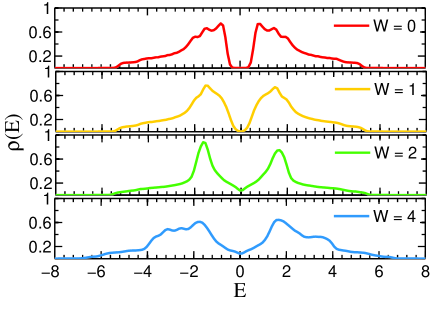
Figure 5: (Color online) Variation of local density of states with disorder strength ranging from $W=0$ (homogeneous) to $W=4$ (highly disordered) with $H_{x}=0.5$ and $\alpha=0.8$ at $T=0$.

With increasing disorder, states begin to appear in the gap and the nature of tunneling spectrum changes rapidly. The single-particle density of state is plotted in Fig. 5 for different disorder strengths. In the homogeneous limit, there is a real gap in the DOS, with the usual pile up of states on both sides of it. With increasing disorder, a pseudo-gap appears, reminiscent of the under-doped high-$T_{c}$ superconductors 0034-4885-62-1-002 ; PhysRevB.71.014514 or a superconductor in presence of high magnetic field PhysRevB.78.024502 . The pile up also smears out and the spectrum is pushed towards higher energy. Therefore, in scanning tunneling microscopy, one would be able to observe regions of real gap with a pile up of states in the DOS, separated by gapless (or pseudo-gapped) non-superconducting regions. These latter regions would also show up clearly in a magnetic force microscopy.

III.0.4 Superfluid Density

To explicitly understand how disorder affects superconductivity and to track the superconductor-insulator transition, one needs to study the superfluid density that characterizes superconducting phase rigidity. We calculate the superfluid density, defined from the effective Drude-weight PhysRevLett.68.2830 ; 0295-5075-34-9-705 , as

$$\rho_{s}\equiv\frac{D_{s}}{\pi e^{2}}=-<K_{x}>+\Pi_{xx}(q\rightarrow 0,\omega\rightarrow 0)$$ (10)

The first term represents the diamagnetic response to an external magnetic field ${\bf{B}}=\nabla\times{\bf{A}}$ with the local kinetic energy

$$\begin{split}K_{x}^{i}=&-t\sum_{n,\sigma}(f(E_{n})[u_{n\sigma}^{*}(r_{i+\hat{x}})u_{n\sigma}(r_{i})+c.c]\\ &+(1-f(E_{n}))[v_{n\sigma}^{*}(r_{i+\hat{x}})v_{n\sigma}(r_{i})+c.c])\end{split}$$ (11)

The second term is the paramagnetic response given by the disorder-averaged transverse current-current correlation function

$$\Pi_{xx}(q\rightarrow 0,\omega\rightarrow 0)=\frac{1}{N}\sum_{ij}\Pi_{xx}^{ij}(\omega=0)$$ (12)

with

$$\begin{split}\Pi_{xx}^{ij}&(\omega=0)\\ &=\sum_{n_{1},n_{2}}A_{n_{1},n_{2}}^{i}[A_{n_{1},n_{2}}^{j*}+D_{n_{1},n_{2}}^{j}]\frac{f(E_{n_{1}})-f(E_{n_{2}})}{E_{n_{1}}-E_{n_{2}}}\end{split}$$ (13)

where

$$\begin{split}&A_{n1,n2}^{i}=2[u_{n_{1}}^{*}(r_{i+\hat{x}})u_{n_{2}}(r_{i})-u_{n_{1}}^{*}(r_{i})u_{n_{2}}(r_{i+\hat{x}})]\\ &D_{n1,n2}^{i}=2[v_{n_{1}}(r_{i+\hat{x}})v_{n_{2}}(r_{i})^{*}-v_{n_{1}}(r_{i})v_{n_{2}}^{*}(r_{i+\hat{x}})]\\ \end{split}$$ (14)

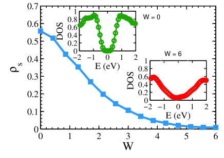
Figure 6: (Color online) Superfluid density as a function of disorder. Insets show the DOS on both sides of the superconducting transition. Parameters used: $T=0$, $H_{x}=0.5$ and $\alpha=0.8$.

Note that the translational invariance is restored via a disorder averaging so that the correlation function is only dependent on the separation $|r_{i}-r_{j}|$. As shown in Fig. 6, the superfluid density $\rho_{s}$ rapidly declines with the strength of disorder, nearly vanishing for $W\simeq 6$ and signifying the proximity of a superconductor to insulator transition driven by disorder. Although quantum phase fluctuations play a crucial role in the superconductor-insulator transition in the large disorder regime PhysRevB.65.014501 ; dubinature2007 , it is beyond the scope of the current approach to incorporate such phase fluctuations. However, from the large suppression of the superfluid density by disorder, we can clearly observe the destruction of superconductivity as disorder strength increases. The sharp decline of stiffness with disorder is understandable in the present situation where there is large spatial fluctuation of the superconducting amplitude. Since the stiffness measures rigidity against phase fluctuations, and in the mean-field BdG theory the phase is uniform throughout, under a phase twist at the boundary the system would accommodate steep adjustments of the phase change in regions where the superconducting amplitude is small. This destroys the overall phase rigidity rapidly over the islands with vanishing gap thereby producing the observed sensitivity to disorder.

III.0.5 Finite Temperature Behaviour

According to scanning squid data Bert2011 , superconductivity, albeit spatially inhomogeneous, appears below a critical temperature. Also, no temperature dependence of the ferromagnetic landscape has been observed over the measured temperature range. On the other hand, the torque magnetometry measurement Li2011 reports a coexistence of ferromagnetism and superconductivity below 120 mK with a superparamagnetic behavior, presumably from the magnetic domains, persisting beyond 200 mK. We therefore undertake a study of the system at finite temperatures with moderate disorder. For a homogeneous system the mean-field superconducting transition can be determined by the condition that the mean superconducting pairing amplitude vanishes. In an inhomogeneous situation, such a criterion is no longer valid. In practice, the superconducting transition is determined by the percolation of the superconducting regions in an insulating matrix, whereas an useful indicator for the transition is the vanishing of the correlation function.

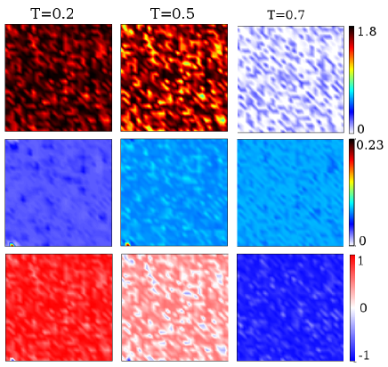
Figure 7: (Color online) The spatial distribution of the local pairing amplitude $|\Delta(r_{i})|$ (top row) and magnetization (middle row). In the bottom row, red and blue represent regions of superconductivity and magnetism respectively. The three columns are for temperature $T=0.2$, $T=0.5$ and $T=0.7$. The lowest row shows coexistence in combined plots of magnetization and local pairing amplitude. The parameters used are $H_{x}=0.5$ and $\alpha=0.8$ at $W=1$.

In Fig. 7, we show the temperature evolution of the spatial distribution of local pairing amplitude, magnetization and their coexistence at different temperatures for a constant disorder strength ($W=1$). The top and middle row show, as in Fig. 2, the development of superconductivity and magnetism separately. With increasing temperature, superconductivity collapses rapidly nearly vanishing by $T=0.7$ (Fig. 7, top row, from left to right), signifying the onset of superconducting transition. Concomitantly, ferromagnetism develops (left to right, middle row) due to the in-plane Zeeman field as the temperature is raised. The coexistence of superconductivity and ferromagnetism is shown in the lowest row of Fig. 7 as temperature rises. Initially superconductivity dominates over the entire system while magnetism shows up in the non-superconducting regions as temperature rises, eventually setting up a near-uniform ferromagnetic state (with small spatial fluctuations) at higher temperatures ($T\simeq 0.7$) in the entire area of the interface.

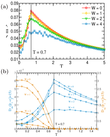
Figure 8: (Color online) Temperature variations of (a) average magnetizations and (b) correlation functions for different disorder strengths. Beyond $T=0.7$, superconducting correlation vanishes. The parameters used: $H_{x}=0.5$, $\alpha=0.8$.

An interesting point to note is that, the average magnetization increases with temperature showing a peak near $T=0.7$ as in Fig. 8(a). This observation is understood from Fig. 8(b), where we plot the correlation functions as a function of temperature. Beyond $T=0.7$, the superconducting correlation is nearly absent, ferromagnetism peaks (albeit with spatial fluctuations due to disorder) and then drops further on. The tail in Fig. 8(a) is extended to higher temperatures depending on the Zeeman field and disorder strength. This picture is quite similar to the torque magnetometry results mentioned above where high temperature magnetism is found to survive beyond the putative superconducting transition temperature.

IV Discussions

Our calculations provide a simple, yet effective description of the superconductivity, ferromagnetism and their coexistence observed at the interface at very low temperatures. We take a phenomenological model for superconductivity PhysRevLett.14.305 ; jourdan2003superconductivity in the presence of local moments along with Rashba SO interaction at the interface, favoring $p_{x}\pm ip_{y}$-wave pairing at finite momentum. The localized moments interact with the itinerant electrons via a ferromagnetic exchange coupling acting like an in-plane Zeeman field. Our calculations reveal that the non-magnetic disorder play a decisive role in the emergence of the coexisting phase where superconductivity and ferromagnetism are phase-separated at microscopic scale. In the homogeneous case, robust ferromagnetism is absent and superconductivity pervades the two-dimensional interface. Ferromagnetism in the interface is facilitated by the disorder: isolated superconducting and insulating regions lead to coexisting superconductivity and magnetism. However at strong disorder, both the phases are affected by large local density fluctuations and tend to disappear. For concreteness, we also study the behaviour of the system at other fillings as depicted in Fig. 9, where we plot the mean pairing ampitude and magnetization in the $n-T$ plane ($n$ is occupation number). As usual, superconductivity has a dome around half-filling and a robust ferromagnetism is established after the superconducting phase is degraded by disorder. However, the phase diagram shows a region of coexistence of an inhomogenous mixture of superconductivity and ferromagnetism.

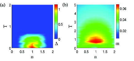
Figure 9: (Color online) Plots of (a) average pairing amplitude and (b) magnetization in the $n-T$ space for fixed disorder strength $W=2$. Parameters used: $H_{x}=0.5$, $\alpha=0.8$.

The general features of magnetism and superconductivity are reasonably well understood in terms of a single band model, although one could envisage a scenario where they occur in different bands as well. The essential physics is disorder-driven and it is possible to explain the coexistence of superconductivity and magnetism within the framework of a single band. Disorder-induced ferromagnetism has also been observed in bulk SrTiO₃ substrate supporting the assertion PhysRevX.2.021014 ; crandles:053908 that there is a definite connection between the presence of impurity and observed ferromagnetism.

Rashba spin-orbit interaction favors an odd pairing superconducting state and a helical alignment of the electron spins without an overall net moment. However, the presence of in-plane exchange interaction and intrinsic disorder are likely to mitigate its effects and prevent such a long range helical magnetic order. Therefore, phase segregation is a natural and most likely outcome as shown. Rashba coupling, in fact, converts the s-wave superconductivity into a chiral p-wave pairing which is very sensitive to non-magnetic disorder. The presence of the in-plane field and the finite momentum pairing then lead to spin precession at different rates (the effect being weak, as the Zeeman field is much weaker than spin-orbit scales) for the partners of the pair depending on the spin-orbit coupling. The dephasing coming from slightly different spin precession rates of the pair and disorder scattering effectively act as a strong pair-breaking mechanism, with disorder affecting fairly dramatically. As shown in Fig. 10, superconductivity is weakly affected by the spin-orbit coupling and while it is degraded, net magnetic moment increases concomitantly at larger spin-orbit coupling.

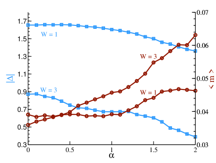
Figure 10: (Color online) Variations of disorder-averaged pairing amplitudes and magnetization with Rashba coupling strength for $W=1$ and $W=3$ with $H_{x}=0.5$ and $T=0$.

The Oxygen vacancies at the interface also have significant influence on the magnetic properties of the interface electrons Schlom2011 ; PhysRevB.85.020407 ; 2013arXiv1311.1791M . There is a quenching of magnetic moment when the system is annealed in Oxygen environment 2013arXiv1305.2226S . An oxygen vacancy presumably adds two additional electrons which are, most probably, partially localized near the vacancy due to Coulomb correlation and the reduction in magnetic moment after annealing is probably due to the reduction of Oxygen vacancies by molecular Oxygen.

Rashba spin-orbit coupling in presence of an applied perpendicular Zeeman field leads to the appearence of spinless ${p_{x}+ip_{y}}$-wave superconductivity which is a canonical example of topological superconductor hosting Majorana bound states under certain conditions PhysRevB.82.134521 ; PhysRevB.79.094504 ; PhysRevB.81.125318 . Since the intrinsic Zeeman field in the system is along the interface plane and brings asymmetry in the Fermi-surface, it is quite unlikely to find any Majorana state here. Moreover, the strong disorder is not conducive to any such topological excitations PhysRevB.83.184520 .

V Conclusions

In the foregoing, we presented a model which elucidates the coexistence of superconductivity and ferromagnetism at the SrTiO₃/LaAlO₃ interface. The presence of gate-tunable Rashba coupling induces chiral $p_{x}\pm ip_{y}$-wave superconductivity and the asymmetric Fermi-surface due to the in-plane Zeeman field favors pairing of electrons at finite momentum. Spatial inhomogeneity at the interface plays a key role in microscopic separation of ferromagnetism and superconductivity and hence the observed coexistence of the two phases. With large disorder, the electronic system segregates into superconducting patches and in the insulating regions local moments order and form ferromagnetic puddles. Our scenario accounts for the scanning squid Bert2011 ; doi:10.1021/nl301451e and magneto-resistance Wang2011 measurements which suggest electronic phase separation in the Ti $d$-bands at the interface.

Similar phenomena of the formation of 2DEG, exhibiting low-temperature superconductivity and ferromagnetism, have also been reported in epitaxially grown GdTiO₃/SrTiO₃ interface 2012PhRvX…2b1014M . The present work provides a unique platform for studying novel interfacial superconductivity and other interesting properties in such heterostructures.

References

- (1) A. Ohtomo and H. Y. Hwang, Nature 427, 423 (2004).
- (2) N. Reyren et al., Science 317, 1196 (2007).
- (3) C. Cen et al., Nat Mater 7, 298 (2008).
- (4) A. D. Caviglia et al., Nature 456, 624 (2008).
- (5) W. M. Lu et al., Applied Physics Letters 99, 172103 (2011).
- (6) C. Bell et al., Phys. Rev. Lett. 103, 226802 (2009).
- (7) D. A. Dikin et al., Phys. Rev. Lett. 107, 056802 (2011).
- (8) L. Li, C. Richter, J. Mannhart, and R. C. Ashoori, Nat Phys 7, 762 (2011).
- (9) J. A. Bert et al., Nat Phys 7, 767 (2011).
- (10) N. Pavlenko, T. Kopp, E. Y. Tsymbal, G. A. Sawatzky, and J. Mannhart, Phys. Rev. B 85, 020407 (2012).
- (11) K. Michaeli, A. C. Potter, and P. A. Lee, Phys. Rev. Lett. 108, 117003 (2012).
- (12) L. Fidkowski, H.-C. Jiang, R. M. Lutchyn, and C. Nayak, Phys. Rev. B 87, 014436 (2013).
- (13) S. Caprara et al., ArXiv e-prints (2013), 1304.2970.
- (14) S. Banerjee, O. Erten, and M. Randeria, Nat Phys 9, 626 (2013), Letter.
- (15) Z. Q. Liu et al., Phys. Rev. X 3, 021010 (2013).
- (16) N. Pavlenko, T. Kopp, E. Y. Tsymbal, J. Mannhart, and G. A. Sawatzky, Phys. Rev. B 86, 064431 (2012).
- (17) D. G. Schlom and J. Mannhart, Nat Mater 10, 168 (2011).
- (18) N. Nakagawa, H. Y. Hwang, and D. A. Muller, Nat Mater 5, 204 (2006).
- (19) A. Savoia et al., Phys. Rev. B 80, 075110 (2009).
- (20) J.-S. Lee et al., Nat Mater 12, 703 (2013).
- (21) S. Yunoki et al., Phys. Rev. Lett. 80, 845 (1998).
- (22) E. Dagotto, T. Hotta, and A. Moreo, Physics Reports 344, 1 (2001).
- (23) L. Santos, T. Neupert, C. Chamon, and C. Mudry, Phys. Rev. B 81, 184502 (2010).
- (24) A. Ghosal, M. Randeria, and N. Trivedi, Phys. Rev. B 65, 014501 (2001).
- (25) Y. Dubi, Y. Meir, and Y. Avishai, Nature 449, 876 (2007).
- (26) B. Chatterjee and A. Taraphder, Solid State Communications 148, 582 (2008).
- (27) M. P. A. Fisher, Phys. Rev. Lett. 65, 923 (1990).
- (28) J. F. Annett, B. L. Györffy, and K. I. Wysokiński, New Journal of Physics 11, 055063 (2009).
- (29) T. Kita, Journal of the Physical Society of Japan 65, 664 (1996).
- (30) M. Stone and I. Anduaga, Annals of Physics 323, 2 (2008).
- (31) D. Ceresoli, T. Thonhauser, D. Vanderbilt, and R. Resta, Phys. Rev. B 74, 024408 (2006).
- (32) A. Ghosal, M. Randeria, and N. Trivedi, Phys. Rev. Lett. 81, 3940 (1998).
- (33) Ariando et al., Nat Commun 2, 188 (2011).
- (34) T. Timusk and B. Statt, Reports on Progress in Physics 62, 61 (1999).
- (35) G. Alvarez, M. Mayr, A. Moreo, and E. Dagotto, Phys. Rev. B 71, 014514 (2005).
- (36) Y. Dubi, Y. Meir, and Y. Avishai, Phys. Rev. B 78, 024502 (2008).
- (37) D. J. Scalapino, S. R. White, and S. C. Zhang, Phys. Rev. Lett. 68, 2830 (1992).
- (38) B. Chattopadhyay, D. M. Gaitonde, and A. Taraphder, EPL (Europhysics Letters) 34, 705 (1996).
- (39) J. F. Schooley et al., Phys. Rev. Lett. 14, 305 (1965).
- (40) M. Jourdan, N. Blümer, and H. Adrian, The European Physical Journal B-Condensed Matter and Complex Systems 33, 25 (2003).
- (41) P. Moetakef et al., Phys. Rev. X 2, 021014 (2012).
- (42) D. A. Crandles, B. DesRoches, and F. S. Razavi, Journal of Applied Physics 108, 053908 (2010).
- (43) N. Mohanta and A. Taraphder, ArXiv e-prints (2013), 1311.1791.
- (44) M. Salluzzo et al., ArXiv e-prints (2013), 1305.2226.
- (45) M. Sato, Y. Takahashi, and S. Fujimoto, Phys. Rev. B 82, 134521 (2010).
- (46) M. Sato and S. Fujimoto, Phys. Rev. B 79, 094504 (2009).
- (47) J. Alicea, Phys. Rev. B 81, 125318 (2010).
- (48) A. C. Potter and P. A. Lee, Phys. Rev. B 83, 184520 (2011).
- (49) B. Kalisky et al., Nano Letters 12, 4055 (2012).
- (50) P. Moetakef et al., Physical Review X 2, 021014 (2012), 1204.1081.