Observability transitions in correlated networks

Abstract

Yang, Wang, and Motter [Phys. Rev. Lett. 109, 258701 (2012)] analyzed a model for network observability transitions in which a sensor placed on a node makes the node and the adjacent nodes observable. The size of the connected components comprising the observable nodes is a major concern of the model. We analyze this model in random heterogeneous networks with degree correlation. With numerical simulations and analytical arguments based on generating functions, we find that negative degree correlation makes networks more observable. This result holds true both when the sensors are placed on nodes one by one in a random order and when hubs preferentially receive the sensors. Finally, we numerically optimize networks with a fixed degree sequence with respect to the size of the largest observable component. Optimized networks have negative degree correlation induced by the resulting hub-repulsive structure; the largest hubs are rarely connected to each other, in contrast to the rich-club phenomenon of networks.

I Introduction

In power-grid networks, the state of a node, i.e., the complex voltage, can be determined by so-called phase measurement units (PMUs; we call them sensors in the following). In a simplified setting, the state of a node is observed if a sensor is placed on the node or its neighbor. In other words, a sensor is capable of measuring the states of a node and its neighborhood. Because measurement is considered to be costly, one is interested in completely or partly observing the nodes in a given network with a small number of sensors Johnson (1974); Raz and Safra (1997). Similar situations may occur in dissemination of information or behavior in social networks. In this case, the sensors correspond to information sources, for example, and a source node may be capable of affecting some neighboring nodes.

Recently, Yang and colleagues formulated this problem by employing the framework of observability transitions Yang et al. (2012). They determined the transition point with respect to the density of sensors above which the largest observable component (LOC) is of a macroscopic size. The results were theoretically derived in the case of random placement of sensors and uncorrelated heterogeneous networks. They also proposed a heuristic algorithm to determine the order in which the nodes receive the sensors for efficient observation of networks with a community structure.

Many networks exhibit degree correlation; the degrees of adjacent nodes are not independent of each other Newman (2002); Serrano et al. (2007). The effect of degree correlation has been investigated for various static and dynamic phenomenological models on networks. Examples include percolation Newman (2002); Vázquez and Moreno (2003); Noh (2007); Goltsev et al. (2008); Shiraki and Kabashima (2010); Herrmann et al. (2011); Schneider et al. (2011); Tanizawa et al. (2012), susceptible-infected-susceptible Eguíluz and Klemm (2002); Boguñá et al. (2003, 2003) and susceptible-infected-recovered Boguñá et al. (2003); Moreno et al. (2003); Hasegawa et al. (2012) models for epidemic spreading, synchronization Wang et al. (2007); Di Bernardo et al. (2007), evolutionary game dynamics Rong et al. (2007); Pusch et al. (2008), and network controllability Pósfai et al. (2013). In particular, degree correlation is known to affect the robustness of networks against random failure of nodes or links. In many network models with degree correlation, negative degree correlation makes the critical node or link occupation probability above which a giant component emerges large, which makes the network less robust Newman (2002); Vázquez and Moreno (2003); Noh (2007); Shiraki and Kabashima (2010).

Motivated by these previous studies, in the present paper we examine the effect of degree correlation on observability transitions. We study the model of network observability transitions proposed in Ref. Yang et al. (2012) in the case of random and degree-based (i.e., hub-first) placement of sensors in uncorrelated and correlated networks. We have good reason to believe that degree correlation is related to observability transitions. To enlarge the LOC for better observability, it is intuitively clear that it is better to avoid allocating sensors to adjacent nodes because such an allocation would yield redundant observation of nodes by multiple sensors. At the same time, nodes in heterogeneous networks are likely to be efficiently observed if we preferentially put sensors on hubs, similar to the role that hubs play in percolation transitions (see Refs. Dorogovtsev et al. (2008); Newman (2010); Cohen and Havlin (2010) for reviews). By combining these two lines of consideration, we postulate that networks with negative degree correlation such that hubs are separated from each other enable efficient observation when the hubs preferentially receive sensors. Even when sensors are sequentially placed on randomly selected nodes, the results may depend on the degree correlation of the network for the same reason.

II Model

For different placement rules and different networks, we study the model introduced in Ref. Yang et al. (2012), which is defined as follows. For a given network, we specify a subset of the nodes that are directly observable by a sensor. We denote the fraction of the directly observable nodes by $\phi$ ($0\leq\phi\leq 1$). Any node adjacent to at least one directly observable node is also observable. We say that such a node is indirectly observable when it is not directly observable. Then, a node is either directly observable, indirectly observable, or unobservable. The problem of finding the smallest set of the directly observable nodes that will make the entire network observable is known as the minimum dominating set problem in graph theory Johnson (1974); Raz and Safra (1997) (also analyzed in Ref. Yang et al. (2012)). Here, similar to the percolation problem, we focus on the size of the LOC, defined as the largest connected component composed of directly or indirectly observable nodes.

III Numerical simulations for networks with degree correlation

In this section, we numerically investigate the relationships between the degree correlation of networks and the size of the LOC. We use scale-free networks, i.e., those with power-law degree distributions, and Poisson networks, i.e., those with the Poisson degree distribution. It should be noted that real power grids do not necessarily have power-law degree distributions Amaral2000 ; Pagani2013 . However, we use scale-free networks to illustrate the effect of generally heterogeneous degree distributions, not to realistically model power grids. In addition, the World Wide Web and social networks, to which observability transitions are expected to be relevant, are scale-free (e.g., Ref. Newman (2010)).

III.1 Generation of networks with a specified degree correlation

We generate scale-free and Poisson networks with a specified degree correlation as follows. First, we generate an uncorrelated network. In the case of scale-free networks, we do so by using a growing network model Krapivsky2000 ; Dorogovtsev et al. (2000); Krapivsky2001a ; Krapivsky2001b . We start with two mutually connected nodes and add nodes one by one until the network has $N$ nodes. Each new node joins the existing network with $m=2$ links. The destinations of the new links are selected from the existing nodes with the probability proportional to $k_{i}+k_{0}$, where $k_{i}$ is the degree of the $i$th existing node and $k_{0}$ is a constant. In this way, we obtain a scale-free network with $p(k)\propto k^{-(3+k_{0}/m)}$ and mean degree $\left<k\right>\approx 2m=4$. Then, we rebuild the network by using the configuration model Newman (2010), with which the links are randomly rewired under the condition that the degree of each node is conserved. In the case of Poisson networks, we use the Erdős-Renyí (ER) random graph on $N$ nodes with $\left<k\right>\approx 4$ as the initial network. We connect each pair of nodes with probability $4/(N-1)$, independently for different pairs.

To introduce degree correlation, we apply to the uncorrelated scale-free or Poisson network a link swapping algorithm Maslov and Sneppen (2002); Xulvi-Brunet and Sokolov (2005); Newman (2010). Specifically, we randomly select two links ($v_{1}$, $v_{2}$) and ($v_{3}$, $v_{4}$) from the current network, where $v_{i}$ ($1\leq i\leq 4$) is a node. Then, we tentatively replace links ($v_{1}$, $v_{2}$) and ($v_{3}$, $v_{4}$) by ($v_{1}$, $v_{3}$) and ($v_{2}$, $v_{4}$). We actually rewire the links if and only if multiple edges and self-loops do not appear after the rewiring and the new network has a more desirable degree correlation than the old network does. Otherwise, we discard the proposed rewiring. In either case, we repeat the rewiring attempts until a network with a targeted degree correlation is realized. It should be noted that the rewiring preserves the degree of each node.

To decide whether to accept a proposed rewiring, we need to quantify the degree correlation. We measure the degree correlation using the Pearson correlation of the excess degree Newman (2002):

$$r=\frac{M^{-1}\sum_{i=1}^{M}K_{i}K_{i}^{\prime}-\left[M^{-1}\sum_{i=1}^{M}\frac{1}{2}\left(K_{i}+K_{i}^{\prime}\right)\right]^{2}}{M^{-1}\sum_{i=1}^{M}\frac{1}{2}\left(K_{i}^{2}+K_{i}^{\prime 2}\right)-\left[M^{-1}\sum_{i=1}^{M}\frac{1}{2}\left(K_{i}+K_{i}^{\prime}\right)\right]^{2}},$$ (1)

where $K_{i}$ and $K_{i}^{\prime}$ are the degrees of the endpoints of the $i$th link ($1\leq i\leq M$), and $M$ is the number of links in the network. It should be noted that $-1\leq r\leq 1$.

III.2 Numerical results

We carry out numerical simulations with scale-free and Poisson networks with different $r$ values. For scale-free networks, we set $p(k)\propto k^{-2.5}$ and generate networks with $r=-0.1$, 0, and 0.1. The absolute values of $r$ for correlated networks are relatively small because it is logically difficult to generate correlated heterogeneous networks with large $|r|$ values; $r$ tends to 0 as $N\to\infty$ Serrano et al. (2007); Alderson and Li (2007); Holme (2007); Menche et al. (2010); Dorogovtsev et al. (2010).

For the entire range of occupation probability $\phi$, the size of the LOC normalized by $N$ under the random placement of sensors is shown in Fig. 1(a). For each value of $r$ and $\phi$, we plotted the size of the LOC averaged over $10^{3}$ realizations of networks. On each realization of the network, we carried out a single run of random placement. Regardless of the degree correlation, the LOC quickly enlarges as $\phi$ increases. For uncorrelated networks, this result is consistent with the previous result Yang et al. (2012). Networks with negative degree correlation (i.e., $r=-0.1$) and uncorrelated networks (i.e., $r=0$) realize slightly larger LOCs than networks with positive degree correlation (i.e., $r=0.1$).

Next, we turn to degree-based placement in which hubs preferentially receive the sensor. The size of the LOC under degree-based placement is shown for scale-free networks with the three $r$ values in Fig. 1(b). The LOC for networks with negative (positive) degree correlation is larger (smaller) than that for uncorrelated networks for most values of $\phi$. The effect of degree correlation is stronger under degree-based placement (Fig. 1(b)) than under random placement (Fig. 1(a)).

The results for Poisson networks under random and degree-based placement are shown in Figs. 1(c) and 1(d), respectively. The results are similar to those for scale-free networks (Figs. 1(a) and 1(b)).

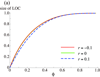
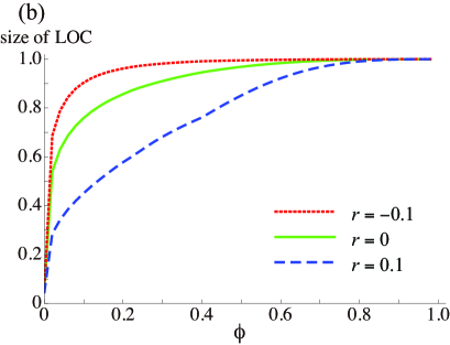
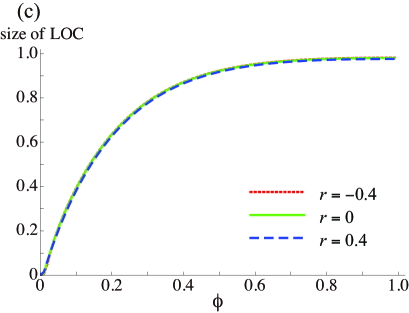
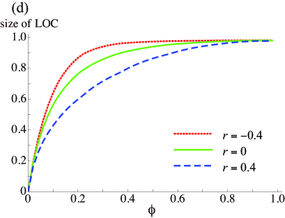
Figure 1: (Color online) Size of the LOC for uncorrelated and correlated networks with $N=10^{4}$. (a) Scale-free networks with $p(k)\propto k^{-2.5}$ under random placement. (b) Scale-free networks with $p(k)\propto k^{-2.5}$ under degree-based placement. (c) Poisson networks under random placement. (d) Poisson networks under degree-based placement. Each data point is an average over $10^{3}$ realizations of the network on each of which a single placement experiment is carried out. It should be noted that we set the final $|r|$ values for correlated networks larger for Poisson networks than scale-free networks, because in scale-free networks it is difficult to continue the rewiring as $|r|$ becomes large (e.g., beyond 0.1 or so), whereas the rewiring when $|r|$ is relatively large is much easier for Poisson networks.

IV Analysis with generating functions

IV.1 Uncorrelated networks

To obtain analytical insights into our numerical results shown in Sec. III.2, in this section we analyze the model by extending the generating function formalism developed in Ref. Yang et al. (2012).

We start with the case of the general order of sensor replacement, including random and degree-based placements, in uncorrelated random and possibly heterogeneous networks. Denote the probability that a node has degree $k$ by $p(k)$. The mean degree is given by $\langle k\rangle=\sum_{k=0}^{\infty}kp(k)$. The probability that an endpoint of a randomly selected link has excess degree, i.e., the number of neighbors minus one, equal to $k$, is given by

$$q(k)=\frac{(k+1)p(k+1)}{\langle k\rangle}.$$ (2)

We define the generating functions for the two distributions as

$$G_{0}(x)= \sum_{k=0}^{\infty}p(k)x^{k},$$ (3)

$$G_{1}(x)= \sum_{k=0}^{\infty}q(k)x^{k}.$$ (4)

We place the sensors on a fraction $\phi$ of nodes in an arbitrary order. To analyze this situation, we define

$$G_{0}(x,{\rm D})=\sum_{k=0}^{\infty}p(k,{\rm D})x^{k},$$ (5)

where $p(k,{\rm D})$ is the probability that a randomly selected node has degree $k$ and is directly observable,

$$G_{0}(x,{\rm nD})=\sum_{k=0}^{\infty}p(k,{\rm nD})x^{k},\\$$ (6)

where $p(k,{\rm nD})$ is the probability that a randomly selected node has degree $k$ and is not directly observable (i.e., indirectly observable or unobservable),

$$G_{1}(x,{\rm D})=\sum_{k=0}^{\infty}q(k,{\rm D})x^{k},\\$$ (7)

where $q(k,{\rm D})$ is the probability that an endpoint of a randomly selected link has excess degree $k$ and is directly observable, and

$$G_{1}(x,{\rm nD})=\sum_{k=0}^{\infty}q(k,{\rm nD})x^{k},$$ (8)

where $q(k,{\rm nD})$ is the probability that an endpoint of a randomly selected link has excess degree $k$ and is not directly observable. It should be noted that

$$G_{0}(1,{\rm D})=1-G_{0}(1,{\rm nD})=\phi$$ (9)

and

$$G_{1}(1,{\rm D})=1-G_{1}(1,{\rm nD})=\tilde{\phi},$$ (10)

where $\tilde{\phi}$ is the probability that an endpoint of a randomly selected link is directly observable.

For adjacent nodes $i$ and $j$, we recursively calculate two quantities. First, $s$ is the probability that $i$ does not connect to the LOC through $j$ under the condition that $i$ is indirectly observable and $j$ is not directly observable (i.e., indirectly observable or unobservable). Second, $u$ is the probability that $i$ does not connect to the LOC through $j$ under the condition that $i$ is directly observable.

We begin by deriving the recursion equation for $s$. Assume that $i$ is indirectly observable. If $j$ is unobservable, $i$ does not connect to the LOC through $j$. This event occurs with probability

$$\frac{1}{1-\tilde{\phi}}\sum_{{k^{\prime}}=0}^{\infty}q({k^{\prime}},{\rm nD})(1-\tilde{\phi})^{{k^{\prime}}}=\frac{1}{1-\tilde{\phi}}G_{1}(1-\tilde{\phi},{\rm nD}).$$ (11)

Because $q({k^{\prime}},{\rm nD})$ is the probability that $j$ has excess degree ${k^{\prime}}$ and is not directly observable, we divided it by $1-\tilde{\phi}$, i.e., the probability that $j$ is not directly observable, to derive the conditional probability. If $j$ is indirectly observable, there are two cases. First, a neighbor of $j$, denoted by $\ell$, is directly observable and does not connect to the LOC with probability $\sum_{{k^{\prime\prime}}=0}^{\infty}q({k^{\prime\prime}},{\rm D})u^{k^{\prime\prime}}=G_{1}(u,{\rm D})$. Second, $\ell$ is not directly observable and does not connect to the LOC with probability $\sum_{{k^{\prime\prime}}=0}^{\infty}q({k^{\prime\prime}},{\rm nD})s=G_{1}(1,{\rm nD})s=(1-\tilde{\phi})s$. Therefore, if $j$ is indirectly observable, $j$ does not connect to the LOC with probability

$$\frac{1}{1-\tilde{\phi}}\sum_{{k^{\prime}}=0}^{\infty}q({k^{\prime}},{\rm nD})\sum_{\overline{k}^{\prime}=1}^{k^{\prime}}\binom{{k^{\prime}}}{\overline{k}^{\prime}}G_{1}(u,{\rm D})^{\overline{k}^{\prime}}\left[(1-\tilde{\phi})s\right]^{k-\overline{k}^{\prime}}$$

$$= \frac{1}{1-\tilde{\phi}}G_{1}(\Psi,{\rm nD})-\frac{1}{1-\tilde{\phi}}G_{1}((1-\tilde{\phi})s,{\rm nD}),$$ (12)

where

$$\Psi=G_{1}(u,{\rm D})+(1-\tilde{\phi})s.$$ (13)

It should be noted that, in Eq. (12), the summation over $\overline{k}^{\prime}$ started with $\overline{k}^{\prime}=1$, not 0, because at least one neighbor of $j$ is directly observable given that $j$ is indirectly observable. By adding the right-hand sides of Eqs. (11) and (12), we obtain

$$s=\frac{1}{1-\tilde{\phi}}G_{1}(1-\tilde{\phi},{\rm nD})+\frac{1}{1-\tilde{\phi}}G_{1}(\Psi,{\rm nD})-\frac{1}{1-\tilde{\phi}}G_{1}((1-\tilde{\phi})s,{\rm nD}).$$ (14)

To derive the recursion equation for $u$, we assume that $i$ is directly observable. The probability that $j$ is directly observable and $i$ does not connect to the LOC through $j$ is equal to $\sum_{{k^{\prime}}=0}^{\infty}q({k^{\prime}},{\rm D})u^{k^{\prime}}=G_{1}(u,{\rm D})$. Otherwise, $j$ is indirectly observable because it is adjacent to $i$, which is directly observable. In the latter case, $i$ does not connect to the LOC through $j$ with probability $G_{1}(\Psi,{\rm nD})$. Therefore, we obtain

$$u=G_{1}(u,{\rm D})+G_{1}(\Psi,{\rm nD}).$$ (15)

Node $i$ is directly observable and belongs to the LOC with probability

$$\sum_{k=1}^{\infty}p(k,{\rm D})(1-u^{k})=\phi-G_{0}(u,{\rm D}).$$ (16)

Node $i$ is indirectly observable and belongs to the LOC with probability

$$\sum_{k=1}^{\infty}p(k,{\rm nD})\sum_{\overline{k}=1}^{k}\binom{k}{\overline{k}}\tilde{\phi}^{\overline{k}}(1-\tilde{\phi})^{k-\overline{k}}\left[1-\left(\frac{G_{1}(u,{\rm D})}{\tilde{\phi}}\right)^{\overline{k}}s^{k-\overline{k}}\right]$$

$$= 1-\phi-G_{0}(\Psi,{\rm nD})-G_{0}(1-\tilde{\phi},{\rm nD})+G_{0}((1-\tilde{\phi})s,{\rm nD}).$$ (17)

It should be noted that $G_{1}(u,{\rm D})/\tilde{\phi}$ is the probability that node $j$ adjacent to node $i$ does not connect to the LOC via any neighbor of $j$, given that $j$ is directly observable. Therefore, the probability that a randomly selected node belongs to the LOC, which is identified by the size of the LOC, denoted by $S$, is given by the summation of the right-hand sides of Eqs. (16) and (17), i.e.,

$$S=1-G_{0}(u,{\rm D})-G_{0}(\Psi,{\rm nD})-G_{0}(1-\tilde{\phi},{\rm nD})+G_{0}((1-\tilde{\phi})s,{\rm nD}).$$ (18)

In the case of random replacement, we set $p(k,{\rm D})=\phi p(k)$, $p(k,{\rm nD})=(1-\phi)p(k)$, $q(k,{\rm D})=\phi q(k)$, $q(k,{\rm nD})=(1-\phi)q(k)$, $G_{0}(x,{\rm D})=\phi G_{0}(x)$, $G_{0}(x,{\rm nD})=(1-\phi)G_{0}(x)$, $G_{1}(x,{\rm D})=\phi G_{1}(x)$, and $G_{1}(x,{\rm nD})=(1-\phi)G_{1}(x)$ to obtain $\tilde{\phi}=\phi$. Then, Eqs. (13), (14), (15), and (18) are reduced to

$$S= 1-\phi G_{0}(u)-(1-\phi)\left[G_{0}(\Psi)+G_{0}(1-\phi)-G_{0}((1-\phi)s)\right],$$ (19)

$$s= G_{1}(1-\phi)+G_{1}(\Psi)-G_{1}((1-\phi)s),$$ (20)

$$u= \phi G_{1}(u)+(1-\phi)G_{1}(\Psi),$$ (21)

where

$$\Psi=\phi G_{1}(u)+(1-\phi)s.$$ (22)

These results agree with those in Ref. Yang et al. (2012).

In the case of degree-based placement, we set

$$p(k,{\rm D})= \begin{cases}p(k)&(k>k_{\rm cut}),\\ \alpha p(k)&(k=k_{\rm cut}),\\ 0&(k<k_{\rm cut}),\end{cases}$$ (23)

$$p(k,{\rm nD})= \begin{cases}0&(k>k_{\rm cut}),\\ (1-\alpha)p(k)&(k=k_{\rm cut}),\\ p(k)&(k<k_{\rm cut}),\end{cases}$$ (24)

$$q(k,{\rm D})= \begin{cases}q(k)&(k>k_{\rm cut}),\\ \alpha q(k)&(k=k_{\rm cut}),\\ 0&(k<k_{\rm cut}),\end{cases}$$ (25)

$$q(k,{\rm nD})= \begin{cases}0&(k>k_{\rm cut}),\\ (1-\alpha)q(k)&(k=k_{\rm cut}),\\ q(k)&(k<k_{\rm cut}),\end{cases}$$ (26)

where $k_{\rm cut}$ is the minimum degree of the node at which the sensor is placed. The fraction of nodes with degree $k=k_{\rm cut}$ that receive sensors, denoted by $\alpha$, is determined by

$$\sum_{k=k_{\rm cut}+1}^{\infty}p(k)+\alpha p(k_{\rm cut})=\phi.$$ (27)

We obtain $S$ by substituting Eqs. (23)–(26) in Eqs. (5)–(8) and calculating Eqs. (14), (15), and (18) with

$$\tilde{\phi}=\sum_{k=k_{\rm cut}+1}^{\infty}q(k)+\alpha q(k_{\rm cut}).$$ (28)

The LOC for the uncorrelated scale-free networks with $p(k)\propto k^{-3}$, where the minimum degree is set to 2, and the ER random graph are shown in Figs. 2(a) and 2(b), respectively. For both random and degree-based placements, the analytical results on the basis of the generation functions (lines) agree very well with those obtained from numerical simulations (symbols). The results for random placement replicate those in Ref. Yang et al. (2012). Degree-based placement only slightly shifts the critical $\phi$ value at which the observability transition occurs. This is mainly because the critical $\phi$ value is small even for random placement Yang et al. (2012). This is in particular the case for the scale-free networks (Fig. 2(a)). However, for both networks, the degree-based placement increases the size of the LOC across a wide range of $\phi$ as compared to the case of random placement.

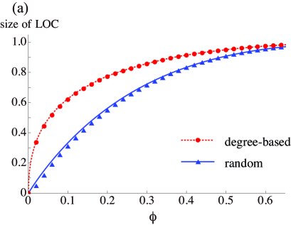
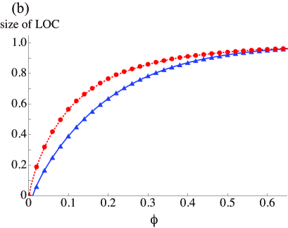
Figure 2: (Color online) Size of the LOC for random and degree-based placements on uncorrelated networks with $N=10^{4}$ and $\left<k\right>\approx 4$. (a) Scale-free networks generated by the configuration model with $p(k)\propto k^{-3}$ ($k\geq 2$). (b) ER random graph. The triangles and circles represent the numerical results for random and degree-based placements, respectively. Each data point is an average value on the basis of 10 realizations of the network. The solid and dotted lines represent the theoretical results for random and degree-based placements, respectively.

IV.2 Correlated networks

In this section, we generalize the theory developed in Sec. IV.1 to the case of networks with degree correlation. To this end, denote by $p(k,{k^{\prime}})$ the probability that the two nodes adjacent to each other through a randomly selected link have degrees $k$ and ${k^{\prime}}$. The normalization is given by $\sum_{k=1}^{\infty}\sum_{{k^{\prime}}=1}^{\infty}p(k,{k^{\prime}})=1$. Denote by $p({k^{\prime}}|k)$ the probability that a neighbor of a node with degree $k$ has degree ${k^{\prime}}$. It should be noted that $\sum_{{k^{\prime}}=1}^{\infty}p({k^{\prime}}|k)=1$ and that $\left[kp(k)/\langle k\rangle\right]p({k^{\prime}}|k)=p(k,{k^{\prime}})=p({k^{\prime}},k)=\left[{k^{\prime}}p({k^{\prime}})/\langle k\rangle\right]p(k|{k^{\prime}})$ Boguñá and Pastor-Satorras (2002); Serrano et al. (2007).

As in Sec. IV.1, we assume that a fraction $\phi$ of nodes selected according to a given order is directly observable. In addition to $p(k,{\rm D})$ and $p(k,{\rm nD})$, we use $p({k^{\prime}},{\rm D}|k)$ and $p({k^{\prime}},{\rm nD}|k)$, which are defined as the probabilities that a neighbor of a node with degree $k$ has degree ${k^{\prime}}$ and is directly observable and not directly observable, respectively. Assume that a node $i$ with degree $k$ and a node $j$ with degree ${k^{\prime}}$ are adjacent to each other. We are going to calculate $s_{k}$, the probability that $i$ is not connected to the LOC through $j$ under the condition that $i$ is indirectly observable and $j$ is not directly observable (i.e., indirectly observable or unobservable), and $u_{k}$, the probability that $i$ is not connected to the LOC through $j$ under the condition that $i$ is directly observable.

Assume that $i$ is indirectly observable. We denote by ${k^{\prime\prime}}$ the degree of node $\ell$, which is a neighbor of $j$ other than $i$. These notations (i.e., ${k^{\prime\prime}}$ and $\ell$) are consistent with those we used in Sec. IV.1. The contribution to $s_{k}$ of the case in which $j$ is unobservable is equal to

$$\frac{1}{\sum_{{k^{\prime}}=1}^{\infty}p({k^{\prime}},{\rm nD}|k)}\sum_{{k^{\prime}}=1}^{\infty}p({k^{\prime}},{\rm nD}|k)\left[\sum_{{k^{\prime\prime}}=1}^{\infty}p({k^{\prime\prime}},{\rm nD}|{k^{\prime}})\right]^{{k^{\prime}}-1}.$$ (29)

When $j$ is indirectly observable, there are two cases. First, $\ell$ is directly observable and does not belong to the LOC with probability $\sum_{{k^{\prime\prime}}=1}^{\infty}p({k^{\prime\prime}},{\rm D}|{k^{\prime}})(u_{k^{\prime\prime}})^{{k^{\prime\prime}}-1}$. Second, $\ell$ is not directly observable and does not belong to the LOC with probability $\sum_{{k^{\prime\prime}}=1}^{\infty}p({k^{\prime\prime}},{\rm nD}|{k^{\prime}})s_{k^{\prime}}$. Therefore, given that $j$ is indirectly observable, it does not belong to the LOC with probability

$$\frac{1}{\sum_{{k^{\prime}}=1}^{\infty}p({k^{\prime}},{\rm nD}|k)}\sum_{{k^{\prime}}=1}^{\infty}p({k^{\prime}},{\rm nD}|k)\sum_{\overline{k}^{\prime}=1}^{{k^{\prime}}-1}\binom{{k^{\prime}}-1}{\overline{k}^{\prime}}\left[\sum_{{k^{\prime\prime}}=1}^{\infty}p({k^{\prime\prime}},{\rm D}|{k^{\prime}})(u_{k^{\prime\prime}})^{{k^{\prime\prime}}-1}\right]^{\overline{k}^{\prime}}\left[\sum_{{k^{\prime\prime}}=1}^{\infty}p({k^{\prime\prime}},{\rm nD}|{k^{\prime}})s_{k^{\prime}}\right]^{{k^{\prime}}-1-\overline{k}^{\prime}}$$

$$= \frac{1}{\sum_{{k^{\prime}}=1}^{\infty}p({k^{\prime}},{\rm nD}|k)}\left\{\sum_{{k^{\prime}}=1}^{\infty}p({k^{\prime}},{\rm nD}|k)(\Psi_{k^{\prime}})^{{k^{\prime}}-1}-\sum_{{k^{\prime}}=1}^{\infty}p({k^{\prime}},{\rm nD}|k)\left[\sum_{{k^{\prime\prime}}=1}^{\infty}p({k^{\prime\prime}},{\rm nD}|{k^{\prime}})s_{k^{\prime}}\right]^{{k^{\prime}}-1}\right\},$$ (30)

where

$$\Psi_{k^{\prime}}=\sum_{{k^{\prime\prime}}=1}^{\infty}p({k^{\prime\prime}},{\rm D}|{k^{\prime}})(u_{k^{\prime\prime}})^{{k^{\prime\prime}}-1}+\sum_{{k^{\prime\prime}}=1}^{\infty}p({k^{\prime\prime}},{\rm nD}|{k^{\prime}})s_{k^{\prime}}.$$ (31)

Using Eqs. (29) and (30), we obtain

$$s_{k}= \frac{1}{\sum_{{k^{\prime}}=1}^{\infty}p({k^{\prime}},{\rm nD}|k)}\left\{\sum_{{k^{\prime}}=1}^{\infty}p({k^{\prime}},{\rm nD}|k)(\Psi_{k^{\prime}})^{{k^{\prime}}-1}+\sum_{{k^{\prime}}=1}^{\infty}p({k^{\prime}},{\rm nD}|k)\left[\sum_{{k^{\prime\prime}}=1}^{\infty}p({k^{\prime\prime}},{\rm nD}|{k^{\prime}})\right]^{{k^{\prime}}-1}\left[1-(s_{k^{\prime}})^{{k^{\prime}}-1}\right]\right\}.$$ (32)

Next, we obtain

$$u_{k}=\sum_{{k^{\prime}}=1}^{\infty}p({k^{\prime}},{\rm D}|k)(u_{k^{\prime}})^{{k^{\prime}}-1}+\sum_{{k^{\prime}}=1}^{\infty}p({k^{\prime}},{\rm nD}|k)(\Psi_{k^{\prime}})^{{k^{\prime}}-1}.$$ (33)

The first term on the right-hand side of Eq. (33) is the probability that $j$ is directly observable and does not belong to the LOC. The second term is the probability that $j$ is indirectly observable and does not belong to the LOC, i.e., $\sum_{{k^{\prime}}=1}^{\infty}p({k^{\prime}},{\rm nD}|k)\left[\sum_{{k^{\prime\prime}}=1}^{\infty}p({k^{\prime\prime}},{\rm D}|{k^{\prime}})(u_{k^{\prime\prime}})^{{k^{\prime\prime}}-1}+\sum_{{k^{\prime\prime}}=1}^{\infty}p({k^{\prime\prime}},{\rm nD}|{k^{\prime}})s_{k^{\prime}}\right]^{{k^{\prime}}-1}$.

Node $i$ is directly observable and belongs to the LOC with probability

$$\sum_{k=1}^{\infty}p(k,{\rm D})\left[1-(u_{k})^{k}\right]=\phi-\sum_{k=0}^{\infty}p(k,{\rm D})(u_{k})^{k}.$$ (34)

Node $i$ is indirectly observable (and hence at least one neighbor of $i$ is directly observable) and belongs to the LOC with probability

$$\sum_{k=1}^{\infty}p(k,{\rm nD})\sum_{\overline{k}=1}^{k}\binom{k}{\overline{k}}\left[\sum_{{k^{\prime}}=1}^{\infty}p({k^{\prime}},{\rm D}|k)\right]^{\overline{k}}\left[\sum_{{k^{\prime}}=1}^{\infty}p({k^{\prime}},{\rm nD}|k)\right]^{k-\overline{k}}\left\{1-\left[\frac{\sum_{{k^{\prime}}=1}^{\infty}p({k^{\prime}},{\rm D}|k)(u_{k^{\prime}})^{{k^{\prime}}-1}}{\sum_{{k^{\prime}}=1}^{\infty}p({k^{\prime}},{\rm D}|k)}\right]^{\overline{k}}(s_{k})^{k-\overline{k}}\right\}$$

$$= 1-\phi-\sum_{k=0}^{\infty}p(k,{\rm nD})\left[\sum_{{k^{\prime}}=1}^{\infty}p({k^{\prime}},{\rm D}|k)(u_{k^{\prime}})^{{k^{\prime}}-1}+\sum_{{k^{\prime}}=1}^{\infty}p({k^{\prime}},{\rm nD}|k)s_{k}\right]^{k}-\sum_{k=0}^{\infty}p(k,{\rm nD})\left[\sum_{{k^{\prime}}=1}^{\infty}p({k^{\prime}},{\rm nD}|k)\right]^{k}\left[1-(s_{k})^{k}\right]$$

$$= 1-\phi-\sum_{k=0}^{\infty}p(k,{\rm nD})(\Psi_{k})^{k}-\sum_{k=0}^{\infty}p(k,{\rm nD})\left[\sum_{{k^{\prime}}=1}^{\infty}p({k^{\prime}},{\rm nD}|k)\right]^{k}\left[1-(s_{k})^{k}\right].$$ (35)

By summing the right-hand sides of Eqs. (34) and (35), we obtain

$$S=1-\sum_{k=0}^{\infty}p(k,{\rm D})(u_{k})^{k}-\sum_{k=0}^{\infty}p(k,{\rm nD})(\Psi_{k})^{k}-\sum_{k=0}^{\infty}p(k,{\rm nD})\left[\sum_{{k^{\prime}}=1}^{\infty}p({k^{\prime}},{\rm nD}|k)\right]^{k}\left[1-(s_{k})^{k}\right].$$ (36)

In the case of random replacement, we use $p(k,{\rm D})=\phi p(k)$, $p(k,{\rm nD})=(1-\phi)p(k)$, $p({k^{\prime}},{\rm D}|k)=\phi p({k^{\prime}}|k)$, $p({k^{\prime}},{\rm nD}|k)=(1-\phi)p({k^{\prime}}|k)$, $\sum_{{k^{\prime}}=1}^{\infty}p({k^{\prime}},{\rm D}|k)=\phi\sum_{{k^{\prime}}=1}^{\infty}p({k^{\prime}}|k)=\phi$, and $\sum_{{k^{\prime}}=1}^{\infty}p({k^{\prime}},{\rm nD}|k)=(1-\phi)\sum_{{k^{\prime}}=1}^{\infty}p({k^{\prime}}|k)=1-\phi$ to simplify Eqs. (31), (32), (33), and (36) as

$$S=1-\phi\sum_{k=0}^{\infty}p(k)(u_{k})^{k}-(1-\phi)\left\{\sum_{k=0}^{\infty}p(k)(\Psi_{k})^{k}+\sum_{k=0}^{\infty}p(k)(1-\phi)^{k}\left[1-(s_{k})^{k}\right]\right\},$$ (37)

where

$$s_{k}= \sum_{{k^{\prime}}=1}^{\infty}p({k^{\prime}}|k)(\Psi_{k^{\prime}})^{{k^{\prime}}-1}+\sum_{{k^{\prime}}=1}^{\infty}p({k^{\prime}}|k)(1-\phi)^{{k^{\prime}}-1}\left[1-(s_{k^{\prime}})^{{k^{\prime}}-1}\right],$$ (38)

$$u_{k}= \phi\sum_{{k^{\prime}}=1}^{\infty}p({k^{\prime}}|k)(u_{k^{\prime}})^{{k^{\prime}}-1}+(1-\phi)\sum_{{k^{\prime}}=1}^{\infty}p({k^{\prime}}|k)(\Psi_{k^{\prime}})^{{k^{\prime}}-1},$$ (39)

and

$$\Psi_{k^{\prime}}=\phi\sum_{{k^{\prime\prime}}=1}^{\infty}p({k^{\prime\prime}}|{k^{\prime}})(u_{k^{\prime\prime}})^{{k^{\prime\prime}}-1}+(1-\phi)s_{k^{\prime}}.$$ (40)

The results for correlated networks obtained so far involve many auxiliary variables, i.e., $s_{k}$ and $u_{k}$. It seems difficult to simplify the results even for the case of random placement (Eqs. (37)–(40)). Therefore, in the rest of this section, we confine ourselves to bimodal networks in which there are only two degree values. Assume that $Na$ and $N(1-a)$ nodes have degrees $k_{1}$ and $k_{2}(<k_{1})$, respectively, such that

$$p(k)=a\delta_{k,k_{1}}+(1-a)\delta_{k,k_{2}}$$ (41)

and

$$\left<k\right>=\sum_{k=k_{1},k_{2}}kp(k)=ak_{1}+(1-a)k_{2},$$ (42)

where $\delta$ is the Kronecker delta. Given a conditional degree distribution $p(k_{1}|k_{2})(=1-p(k_{2}|k_{2}))$, the other conditional degree distribution is automatically determined as $p(k_{2}|k_{1})=k_{2}(1-a)p(k_{1}|k_{2})/ak_{1}(=1-p(k_{1}|k_{1}))$. The degree correlation is equal to

$$r=1-\frac{\left[ak_{1}+(1-a)k_{2}\right]p(k_{1}|k_{2})}{ak_{1}}.$$ (43)

In the case of random placement, we use Eqs. (37)–(40), which involve four recursively calculated variables $s_{k_{1}}$, $s_{k_{2}}$, $u_{k_{1}}$, and $u_{k_{2}}$. In the case of degree-based placement, for $0\leq\phi\leq a$, we use $p(k_{1},{\rm D})=\phi$, $p(k_{1},{\rm nD})=a-\phi$, $p(k_{2},{\rm D})=0$, $p(k_{2},{\rm nD})=1-a$, $p(k_{1},{\rm D}|k_{1})=p(k_{1}|k_{1})\phi/a$, $p(k_{1},{\rm nD}|k_{1})=p(k_{1}|k_{1})\left[1-(\phi/a)\right]$, $p(k_{2},{\rm D}|k_{1})=0$, $p(k_{2},{\rm nD}|k_{1})=p(k_{2}|k_{1})$, $p(k_{1},{\rm D}|k_{2})=p(k_{1}|k_{2})\phi/a$, $p(k_{1},{\rm nD}|k_{2})=p(k_{1}|k_{2})\left[1-\phi/a\right]$, $p(k_{2},{\rm D}|k_{2})=0$, and $p(k_{2},{\rm nD}|k_{2})=p(k_{2}|k_{2})$. We substitute these equations in Eqs. (31), (32), (33), and (36) to obtain $S$ for $0\leq\phi\leq a$. For $a<\phi\leq 1$, we use $p(k_{1},{\rm D})=a$, $p(k_{1},{\rm nD})=0$, $p(k_{2},{\rm D})=\phi-a$, $p(k_{2},{\rm nD})=1-\phi$, $p(k_{1},{\rm D}|k_{1})=p(k_{1}|k_{1})$, $p(k_{1},{\rm nD}|k_{1})=0$, $p(k_{2},{\rm D}|k_{1})=p(k_{2}|k_{1})(\phi-a)/(1-a)$, $p(k_{2},{\rm nD}|k_{1})=p(k_{2}|k_{1})(1-\phi)/(1-a)$, $p(k_{1},{\rm D}|k_{2})=p(k_{1}|k_{2})$, $p(k_{1},{\rm nD}|k_{2})=0$, $p(k_{2},{\rm D}|k_{2})=p(k_{2}|k_{2})(\phi-a)/(1-a)$, and $p(k_{2},{\rm nD}|k_{2})=p(k_{2}|k_{2})(1-\phi)/(1-a)$.

The size of the LOC for uncorrelated and correlated bimodal networks is shown in Fig. 3. Because we set $k_{1}=16$, $k_{2}=2$, and $a=1/7$, we obtain $\left<k\right>=4$. By combining Eq. (43) and $0<p(k_{1}|k_{2})<1$, we obtain $-3/4<r<1$. We set $r=-0.6$, 0, and 0.6 in Fig. 3. In the figure, the numerical results are shown by circles, squares, and triangles. They are calculated for random bimodal networks possessing $N=10^{4}$ nodes, and the size of the LOC at each $\phi$ value is an average over 10 realizations of networks. For both random placement (Fig. 3(a)) and degree-based placement (Fig. 3(b)), the numerical results agree very well with the analytical results derived from the generating functions shown by the lines. The effect of the degree correlation on the size of the LOC is small under random replacement. In contrast, the degree correlation considerably changes the size of the LOC under degree-based placement. However, the critical $\phi$ value does not depend much on the degree correlation even in the case of degree-based placement. These results are qualitatively the same as those for scale-free and Poisson networks shown in Fig. 1. It should be noted that the increase in the size of the LOC is not smooth at $\phi=a=1/7$ under degree-based placement (most evident for $r=0$; solid line in Fig. 3(b)) because the analytical expression for the LOC size changes at $\phi=a$.

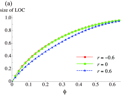
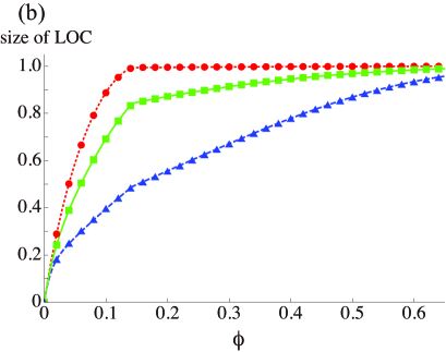
Figure 3: (Color online) LOC size for bimodal networks with $k_{1}=16$, $k_{2}=2$, and $a=1/7$. (a) Random placement. (b) Degree-based placement. The dotted, solid, and dashed lines represent the theoretical results obtained with the generation functions for $r=-0.6$, $r=0$, and $r=0.6$, respectively. The circles, squares, and triangles represent the numerical results for $r=-0.6$, $r=0$, and $r=0.6$, respectively.

V Networks optimized for the size of the LOC

To support our claim that negative degree correlation enlarges the observable component, we numerically explore optimal network structure for observability transitions under degree-based placement. The results shown in the previous sections indicate that degree-based placement considerably enhances the size of the LOC for a wide range of $\phi$, whereas it does not change the critical $\phi$ value much. Therefore, similar to the analysis of the percolation transition Herrmann et al. (2011); Schneider et al. (2011); Tanizawa et al. (2012), we define the objective function to be optimized as the size of the LOC summed over $\phi$ values, i.e.,

$$R_{\rm O}=\frac{1}{N+1}\sum_{i=0}^{N}O(i),$$ (44)

where $O(i)$ ($0\leq O(i)\leq 1$) is the relative size of the LOC when the sensors are placed on the first $i(=N\phi)$ nodes in the descending order of degree. It should be noted that $O(0)=0$ and $O(1)=1$.

Herrmann and colleagues used an optimization method to generate the most tolerant network against the targeted (i.e., degree-based) attack Herrmann et al. (2011); Schneider et al. (2011) (also see Tanizawa et al. (2012)). They optimized a given network by repetitively rewiring two randomly selected links without changing the degree of each node, if the rewiring increased a tolerance measure. We carry out a similar optimization experiment as follows. First, we prepare uncorrelated networks according to the configuration model or the ER random graph. Second, we select two links at random and tentatively rewire them in the same manner as the method for generating correlated networks (Sec. III.1). If the tentative rewiring increases $R_{\rm O}$, we adopt the rewiring if it does not yield multiple links or self-loops. Otherwise, we discard the proposed rewiring. We repeat the tentative rewiring, including unsuccessful attempts, $10^{7}$ times. We set $N=10^{4}$.

The $R_{\rm O}$ values before and after the optimization of the scale-free network with $p(k)\propto k^{-2.5}$ and $\left<k\right>\approx 4$ are equal to 0.9178 $\pm$ 0.0015 and 0.9943 $\pm$ 0.0003 (mean $\pm$ standard deviation), respectively, where the statistical values are calculated on the basis of 10 realizations of networks. The optimization procedure considerably increases the size of the LOC. The results are qualitatively the same for Poisson networks. The $R_{\rm O}$ values before and after the optimization are equal to 0.8493 $\pm$ 0.0014 and 0.9247 $\pm$ 0.0011, respectively.

The optimization in terms of the LOC does not enlarge the conventional percolation cluster. To show this, we measure the order parameter $R_{\rm D}\equiv\sum_{i=0}^{N}D(i)/(N+1)$, where $D(i)$ is the normalized size of the largest connected component (LCC) when the $i$ nodes are occupied in the descending order of degree of the original network. By definition, $R_{\rm D}$ is large if the LCC composed of the directly observable nodes is large for a wide range of $\phi$. $R_{\rm D}$ is analogous to the one previously used for analyzing targeted attacks Herrmann et al. (2011); Schneider et al. (2011); Tanizawa et al. (2012) and summarizes the size of the LCC across various values of $\phi$. If $R_{\rm D}$ is large, placing the sensor on a relatively small number of nodes can make the LCC large. Throughout the optimization procedure in terms of the LOC described above, $R_{\rm D}$ changes from 0.4937 $\pm$ 0.0005 to 0.4990 $\pm$ 0.0001 for scale-free networks. The size of the LCC is close to 0.5, which is the maximum possible value realized when $D(i)=i/N$, even before the optimization. Partly for this reason, the increase in $R_{\rm D}$ is small albeit significant. For Poisson networks, $R_{\rm D}$ significantly decreases from 0.4909 $\pm$ 0.0007 to 0.4722 $\pm$ 0.0003 through the optimization in terms of $R_{\rm O}$.

For scale-free networks with different $\gamma$ values and the ER random graph, the degree correlation after the optimization is shown in Fig. 4 (circles). The $r$ values corresponding to $\gamma=\infty$ indicate the results for the ER random graph. The optimized networks have negative $r$ values irrespective of the degree distribution. This result is consistent with those obtained in Sec. III.2. The negative $r$ value is not caused by the fact that scale-free networks with small $\gamma$ have inherently negative $r$ values  Maslov et al. (2004); Park and Newman (2003); Boguñá et al. (2004); Catanzaro et al. (2005); Alderson and Li (2007); Weber and Porto (2007); Serrano et al. (2007); we confirmed that $r$ did decrease as a result of optimization for any $\gamma$.

To contrast the negative degree correlation emerging as a result of the optimization in terms of $R_{\rm O}$, we also carried out another set of numerical optimization experiments. We optimized the scale-free and Poisson networks in terms of $R_{\rm D}$. The $r$ values after the optimization, shown by the squares in Fig. 4, have different signs depending on the degree distribution. In general, highly heterogeneous networks tend to produce negative $r$ even if they are constructed from the configuration model Maslov et al. (2004); Park and Newman (2003); Boguñá et al. (2004); Catanzaro et al. (2005); Alderson and Li (2007); Weber and Porto (2007); Serrano et al. (2007). The theory suggests that this phenomenon occurs only for $\gamma<3$ Boguñá et al. (2004). These previous results are consistent with the results shown in Fig. 4. Therefore, we conclude that the LCC tends to be large with positive degree correlation, whereas the LOC tends to be large with negative degree correlation.

Finally, the adjacency matrices obtained after the optimization in terms of $R_{\rm O}$ are shown in Figs. 5(a) and 5(b) for a scale-free network with $p(k)\propto k^{-3}$ and a Poisson network, respectively. In each panel, the nodes are arranged in the ascending order of degree. The vertical and horizontal solid lines separate the degree groups such that the nodes that fall in the same partition have the same degree. This grouping is done only for small values of $k$ for clarity. Figures 5(a) and 5(b) indicate that the optimized networks have little direct connection between a certain number of the largest hubs. This is the main reason for the negative degree correlation observed in Fig. 4.

We do not apparently see much structure in the adjacency matrices shown in Figs. 5(a) and 5(b) except that hubs are not adjacent. This result is in contrast with the connectivity matrices for other negatively correlated networks, such as networks with maximally negative degree correlation Menche et al. (2010), fractal networks Song et al. (2006), and other hub-repulsive real-world networks Maslov and Sneppen (2002); Maslov et al. (2004). We consider that the adjacency matrices shown in Figs. 5(a) and 5(b) are produced for the following intuitive reason. Once a sufficient number of the largest hubs receive sensors, most of the remaining nodes are indirectly observed through a hub such that the details of the connectivity between the remaining nodes little contribute to the size of the LOC. With this density of sensors, the neighborhoods of hubs would be adjacent to each other to make the LOC large. The number of hubs that are repulsive to each other can be estimated as follows. A sensor located at node with degree $k$ makes $k+1$ nodes observable. Because a large $R_{\rm O}$ value implies that the size of the LOC reaches $\approx N$ at a small $\phi$ value, the minimum degree of the node with the sensor, denoted by $k_{i_{0}}$ is estimated to be the largest $i_{0}$ such that $\sum_{i=i_{0}}^{N}(k_{i}+1)$ exceeds $N$, where the nodes are arranged in the ascending order of degree. The $i_{0}$ values estimated in this manner are shown by the dotted lines in Fig. 5. The estimation accurately describes the number of hubs that are not adjacent to each other.

This estimation method implicitly assumes that hubs are separated by distance three. Otherwise, the neighborhoods of different directly observable nodes would overlap even at small $\phi$. Such an overlap leads to a redundant usage of sensors. To verify this point, we plot the so-called connectivity matrix with distance two for the scale-free and Poisson networks in Figs. 5(c) and 5(d), respectively. By definition, the ($i,j$) entry of this matrix is equal to unity if nodes $i$ and $j$ are connected with distance two and zero otherwise. Figures 5(c) and 5(d) indicate that the largest hubs are less frequently connected with each other than other node pairs with distance two as well as node pairs with distance one. This result justifies our estimation method for $i_{0}$.

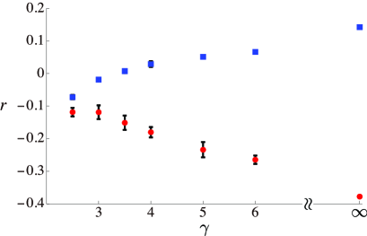
Figure 4: (Color online) Degree correlation after the optimization. We set $N=10^{4}$. The circles and squares correspond to the results for the optimization in terms of $R_{\rm O}$ and $R_{\rm D}$, respectively. We denote by $\gamma$ the scale-free exponent of the degree distribution (i.e., $p(k)\propto k^{-\gamma}$), and $\gamma=\infty$ corresponds to Poisson networks. Error bars are the standard deviations on the basis of 10 realizations. They are smaller than the size of the circle when $\gamma=\infty$ and the squares for all the $\gamma$ values.

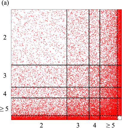
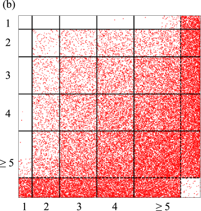
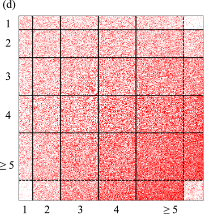
Figure 5: (Color online) Connectivity matrices after the optimization in terms of $R_{\rm O}$. (a) Adjacency matrix for an optimized scale-free network with $p(k)\propto k^{-3}$. A dot indicates that the corresponding node pair is adjacent. The nodes are arranged in the ascending order of degree. The blocks separated by solid lines represent different degree classes. The nodes in the same block have the same degree except that we merged the nodes with large degrees into one block. The dotted lines represent node index $i_{0}$ determined by $\sum_{i=i_{0}}^{N}(k_{i}+1)\approx N$. (b) Adjacency matrix for an optimized Poisson network. The nodes with $k=0$ are not shown. For both networks, we set $N=10^{4}$. (c) Connectivity matrix with distance two for the optimized scale-free network shown in (a). A dot indicates that the corresponding node pair is connected with distance two. (d) Connectivity matrix with distance two for the optimized Poisson network shown in (b).

VI Discussion

We examined observability transitions in correlated networks. We showed that the LOC is larger for various values of the sensor density (i.e., $\phi$) for networks with negative degree correlation than those with null or positive degree correlation under both random and degree-based placement protocols. The effect of the degree correlation is more pronounced for degree-based than for random placement.

In percolation transitions on networks, negative degree correlation tends to shift the percolation threshold such that emergence of the giant component requires a larger occupation probability of nodes or links in negatively correlated networks Newman (2002); Vázquez and Moreno (2003); Noh (2007). Links between hubs are beneficial in maintaining a large connected component at least near the percolation threshold. In contrast, in the model of observability transitions, negative degree correlation increases the size of the LOC even in the case of random placement. Links between hubs are now detrimental owing to overlap of the neighborhoods of hubs, which implies redundant usage of the sensors. If pairs of hubs are within distance three, the hubs’ neighborhoods are easily connected, resulting in a large LOC.

Networks optimized in terms of the size of the LOC under degree-based sensor placement have negative degree correlation. In fact, the main cause of the negative degree correlation is the extremely hub-repulsive structure of the final networks (Fig. 5). This structure is distinct from that of other types of networks with negative degree correlation. First, the networks with maximally negative correlation in terms of $r$ have a bilayer structure Menche et al. (2010). In these networks, the nodes with the smallest degrees are exclusively connected with the largest hubs, those with the second smallest degrees are exclusively connected with the largest hubs among the remaining nodes, and so on. Second, fractal networks also have negative degree correlation Yook et al. (2005); Song et al. (2006); Rozenfeld et al. (2007); Guimera et al. (2007); Palotai et al. (2008). However, the so-called correlation profile, i.e., an averaged adjacency matrix in which the nodes are ordered in the ascending order of degree, for fractal networks Song et al. (2006) is not similar to the adjacency matrices for our optimized networks (Figs. 5(a) and 5(b)). The protein interaction and gene regulatory networks in yeast Maslov and Sneppen (2002) and the Internet Maslov et al. (2004) also have the hub-repulsive property, but their correlation profiles at small degree nodes are quite different from those of our optimized networks. The fact that our optimized networks are different from these negatively correlated networks is consistent with the fact that the $r$ value alone does not specify the network structure Alderson and Li (2007); Serrano et al. (2007); Weber and Porto (2007); Whitney and Alderson (2008); Menche et al. (2010); Dorogovtsev et al. (2010).

The rich-club phenomenon is a property of networks in which hubs are densely interconnected as compared to other pairs of nodes Zhou and Mondragón (2004); Colizza et al. (2006). In contrast, links between hubs are extremely underrepresented in our optimized networks. Therefore, our optimized networks could be said to show an anti-rich-club phenomenon. In fact, the hub-repulsive structure has been suggested to be the inverse of the rich-club phenomenon Palotai et al. (2008). Further investigation of this network structure and its relevance to other phenomena and applications warrants future work.