Axisymmetrically Tropical Cyclone-like Vortices with Secondary Circulations

Abstract

The secondary circulation of the tropical cyclone (TC) is related to its formation and intensification, thus becomes very important in the studies. The analytical solutions have both the primary and secondary circulation in a three-dimensionally nonhydrostatic and adiabatic model. We prove that there are three intrinsic radiuses for the axisymmetrically ideal incompressible flow. The first one is the radius of maximum primary circular velocity $r_{m}$. The second one is radius of the primary kernel $r_{k}>r_{m}$, across which the vorticity of the primary circulation changes sign and the vertical velocity changes direction. The last one is the radius of the maximum primary vorticity $r_{d}$, at which the vertical flow of the secondary circulation approaches its maximum, and across which the radius velocity changes sign. The first TC-like vortex solution has universal inflow or outflow. The relations between the intrinsic length scales are $r_{k}=\sqrt{2}r_{m}$ and $r_{d}=2r_{m}$. The second one is a multi-planar solution, periodically in $z$-coordinate. Within each layer, the solution is a convection vortex. The number of the secondary circulation might be one, two, three, and even more. There are also three intrinsic radiuses $r_{m}$, $r_{k}$ and $r_{d}$, but they have different values. It seems that the relative stronger radius velocity could be easily found near boundaries. The above solutions can be applied to study the radial structure of the tornados, TCs and mesoscale eddies.

Keywords: Tropic cyclone, vortex, Secondary Circulation, nonhydrostatic, intrinsic radius

1 Introduction

Typhoons (hurricanes or tropical cyclones) are intense atmospheric cyclonic vortices that genesis over warm tropical oceans with their energy primarily from the release of water vapor latent heat. As the tropical cyclones (hereafter TCs) could make great impacts on both oceanic and terrestrial environments, there were lots of investigations on all the relative issues. Among them, a very fundamental problem is understanding the three-dimensional structures and dynamics of the TC, which is useful for both weather forecasters and researchers. In this problem, the thermal dynamics (moisture convection) and the mechanic dynamics are strongly coupled, which could hardly be solved theoretically.

According to the observations, the TC has a strong cyclonic circulation (primary circulation), and a weak vertical circulation (secondary circulation). The inner part of the storm becomes nearly axisymmetric as the storm reaches maturity, and its strongest winds surround a relatively calm eye, whose diameter is typically in the range of 20 to 100 km ChanBook2010. Nolan2002 pointed out that the TC can be represented to zeroth order as a vortex in gradient wind and hydrostatic balance, with no secondary circulation. In most theoretical studies, the ideal axisymmetric and steady-state model was used. The model is based on the assumptions that the flow above the boundary layer is inviscid and thermodynamically reversible, that hydrostatic and gradient wind balance could apply Emanuel1986; Stern2009. As a first step in the prediction of the TC track, the TC is taken as a barotropic vortex. In some cases, a simple two-dimensional barotropic dry model is used to simulate a TC-like concentric rings vortex Mallen2005; Martinez2010; Moon2010. Mallen2005 compared the different approximation of the primary circulation with the observed data. The primary circulation far away from the inner core is like a Rankine with skirt vortex.

Another important feature of TC is the secondary circulations. The secondary circulation is coupled to the vertical motion induced by the convection that drives the vortex. Inside the radius of maximum winds, where the radial inflow erupts out of the boundary layer, vertical velocities are comparable to those in the overhead convection Nolan2002. The secondary circulation has related to TC formation and intensification in idealized flow configurations Montgomery2006; Kieu2009; Montgomery2011qj. Due to the complexity of the problem, Nolan2002 can only compute the solutions of three-dimensional linear perturbations on a primary circulation to study the secondary circulation. Kieu2009 studied the evolution of a Rankine vortex with exponential growth in the core region. However, due to the neglect of both the vertical momentum equation and the thermodynamic equation, the exponential growth rate of the TC seems to fast to accept Montgomery2010qj.

Though lots of works dealing with this problem, the dynamics and the structure of the secondary circulation is far to a fine diagram. In the schematic diagram of model for a mature steady-state hurricane Emanuel1986, the secondary circulation is divided into three regions along radius. The inner eye is Region I, then Region II is the eyewall cloud, the outer to far is Region III. The model assumes that the radius of maximum tangential wind speed, $r_{m}$, is located at the outer edge of the eyewall cloud, whereas the recent observations indicate it is closer to the inner edge Montgomery2011qj.

As an alternative way to avoid the above disadvantage, we consider to solve a nonhydrostatic and adiabatic model following the deviation by Batchelor1967; Frewer2007 and to apply separation of variables by SunL2011taml; SunL2011arx. In this study, we use the nonlinear Euler equations following the assumptions by Emanuel1986. And we consider the axisymmetric vortices in a rotation plane with the constant Coriolis parameter $f$ ($f$-plane). In the inner part of the TC (e.g. the radius less than 50 km), the gradient balance dominates the primary circulation Willoughby1990Jas. As a result, a general exact spiral solution is presented in § 2, some three-dimensional TC-like vortex solution with secondary circulation solutions are given in § 3. Discussion and conclusion are respectively given in § 4 and in § 5, respectively.

2 General solution

Different from the previous studies, a nonhydrostatic model is employed to study the secondary circulation. We consider the steady solutions of the incompressible Euler equations for axisymmetric flow in a rotation plane. The constant $f$ represents the Coriolis parameter due to rotation. It is convenient to use a cylindrical coordinate system $(r,\theta,z)$ with the velocity components ($V_{r},V_{\theta},V_{z}$), and all the velocity components are the functions of $r$ and $z$ but $\theta$, due to the axisymmetric. As $V_{r}=V_{r}(r,z)$, $V_{\theta}=V_{\theta}(r,z)$ and $V_{z}=V_{z}(r,z)$, the governing equations, including mass-conservation and momentum equations, are: ∂(rVr)∂r + ∂(rVz)∂z &=0
V_r∂Vθ∂r + V_z∂Vθ∂z+VrVθr +fV_r =0
V_r∂Vr∂r + V_z∂Vr∂z-Vθ2r-f V_θ -14f^2r =-1ρ∂p∂r
V_r∂Vz∂r + V_z∂Vz∂z =-1ρ∂p∂z The last one is nonhydrostatic balance in vertical direction. The solution of above system has two parts, the rigid rotation $(V^{0}_{r},V^{0}_{\theta},V^{0}_{z})=(0,-\frac{1}{2}fr,0)$ and the three-dimensional flow $(V^{1}_{r},V^{1}_{\theta},V^{1}_{z})$ represented by an axisymmetric stream function $\Psi(r,z)$. A typical value of the rigid rotation is $\frac{1}{2}fr=1m/s$ for $f=5\times 10^{-5}s^{-1}$ at $20^{o}N$ and $r=2\times 10^{4}m$, which is relatively small than the three-dimensional flow. It should be noted that there is no length scale for $\Psi(r,z)$ in Eq.(2), thus the solution of $\Psi(r,z)$ can be uniformly stretched by simply multiplying a real constant $a$. We tried to find the solution of the above equations by separation of variables $\Psi(r,z)=R(r)H(z)$. One such solution can be written as,

$$V_{r}=\frac{R(r)}{r}H^{\prime}(z),\,\,V_{\theta}=\mu\frac{R(r)}{r}H(z)-\frac{1}{2}fr,\,\,V_{z}=-\frac{R^{\prime}(r)}{r}H(z)$$ (1)

where ^′ presents first deviation and $\mu$ is a real constant. The absolute angular momentum $M$ of the primary circulation is defined as,

$$M=rV_{\theta}+\frac{1}{2}fr^{2}=\mu\Psi(r,z)$$ (2)

So the constant $\mu$ is the ratio of the primary circulation’s absolute angular momentum to the secondary circulation flow streamfunction. As the $M$ is a function only $\Psi$ belong, we have the following principle (see Appendix for proof).

Theorem 1: For axisymmetrically incompressible ideal flow, there is an intrinsic radius $r_{k}$, within which is the kernel of the primary vortex. The vortex boundary $r_{k}$ is the frontier of the positive and negative vorticity of the primary circulation, and also the frontier of upward and downward flows of the secondary circulation. The maximum velocity of the primary circulation locates within the vortex kernel, i.e., the radius of maximum wind (RMW in TC studies, namely $r_{m}$) $r_{m}<r_{k}$.

The ratio of two different parts of the primary circulation is the Rossby number

$$Ro=\frac{V^{1}_{\theta}}{V^{0}_{\theta}}=\frac{2\mu R(r)}{fr^{2}}H(z)$$ (3)

The radius of the inner part of the TC is typically in the range of 10 to 50 km Stern2009; ChanBook2010, and the typical value of $f$ is $5\times 10^{-5}s^{-1}$ at $20^{o}N$. So the typical value of $Ro\gg 1$ within this regime for a TC, and the rotation effect could be approximately ignored for the inner part. In the outer part of the TC, especially far from the TC core, the Rossby number $Ro\ll 1$ and the rigid rotation is concern. It is from Eq.(3) that the flow might be geostrophic if $H(z)\rightarrow 0$ at a certain depth. In present work, both $V^{0}_{\theta}$ and $V^{1}_{\theta}$ are obtained analytically, but only the second one is nontrivial.

For the given stream function $\Psi(r,z)$, equation (2a) and equation (2b) are satisfied automatically. The path of a fluid material element can be obtained, lnr(θ) &= 1μH’Hθ
Ψ(r,z) = const. In $r-\theta$ plan, it is a logarithmic spiral ($H^{\prime}\neq 0$), except for $H^{\prime}=0$ (a circle). So we called the solution is spiral solution. In fact, the path is right on a Bernoulli surface given by Eq.(2b), on which the streamfunction is defined Batchelor1967. As the ideal flow satisfies the Bernoulli s theorem, the total energy $E$ is conserved, and can only be a function of $\Psi$ alone, a simple relation being

$$\frac{dE}{d\Psi}=4k^{4}\rho\Psi$$ (4)

where $k$ is a constant. If $k=0$, the total energy is homoenergetic. While the total energy is proportion to the kinetic energy for $k\neq 0$, and the pressure is also proportion to the kinetic energy.

It is noted that there are only two constants ($\mu$ and $k$) constraining the problem. For any given pair of $\mu$ and $k$, there might be different solutions for different $H(z)$ (e.g., Eq.(19) in Appendix) and $R(r)$ (e.g., Eq.(LABEL:Eq:Axisflow-velsol-R,gamma!=0) in Appendix). With the solution of $R(r)$ and $H(z)$ (see Appendix for detail), the streamfunction is $\Psi(r,z)=aR(r)H(z)$. In the following section, we simply let $a=1$ or $a=-1$ without changing the universality, as it is mentioned above.

3 Special solutions

3.1 Mono-layer solution

Figure 1: Paths of the fluid material elements for the TC-like vortex. (a) $r-\theta$ plane for inflow, (b) $r-\theta$ plane for outflow, (c) the secondary circulation in $z-r$ plane, (d) the fluid material elements within the vortex near the kernel.

In this case, the solution of $\Psi(r,z)=ar^{2}e^{-\lambda z-k^{2}r^{2}}$ is finite within the whole domain, if we choose appropriate $\lambda<0$ for $z<0$ and $\lambda>0$ for $z>0$. If taking $\lambda>0$ for $z>0$, the radial velocity $V_{r}$ does not change its direction within the domain. Thus the secondary flow is either inflow or outflow depending on the constant $a$ (Fig 1a,b). The smaller $\lambda$ is, the higher the flow could be, as the velocity is e-fold decline in $z$ direction. Besides, there are the standard horizontal length scale $r_{s}$ and the vertical length scale $h$, which are defined from the e-fold vertical function,

$$r_{s}=1/k,h=1/\lambda.$$ (5)

The standard aspect ratio $A_{s}$ of the vertical length scale to the horizontal length scale is,

$$A_{s}=h/r_{s}=k/\lambda.$$ (6)

The velocities are, Vr&= λre-λz-k2r2,
Vθ=±8k2-λ2 re-λz-k2r2-12fr,
Vz= 2(1-k2r2)e-λz-k2r2.

For the primary circulation, the circular velocity of $V^{1}_{\theta}$ is the same with that of the Taylor vortex for any fixed $z$, by ignoring the rigid rotation flow $V^{0}_{\theta}$. The circular velocity maximum is $V^{1}_{\theta m}=\sqrt{8k^{2}-\lambda^{2}}r_{m}e^{-\lambda z-\frac{1}{2}}$ at $r_{m}^{2}=1/(2k^{2})$, which is free of the constants $a$, $\mu$ and $\lambda$. With the $r_{m}$ and $V^{1}_{\theta m}$, the circular velocity could be represent as,

$$V^{1}_{\theta}=V^{1}_{\theta m}r_{*}e^{\frac{1}{2}(1-r_{*}^{2})},r_{*}=r/r_{m}$$ (7)

If the rigid rotation is taken into consideration under the condition of $Ro\ll 1$ as $e^{-\lambda z}\ll 1$. This might occurs at very high level for smaller $\lambda$ or very low level for larger $\lambda$. the radius $r_{m}$ is slant inside ($V^{1}_{\theta}<0$) or outside ($V^{1}_{\theta}>0$) along $z$. This can be seen from the observation data Stern2009. Besides, the primary circulation vorticity approaches to its maximum at $r_{d}=2r_{m}$, where the secondary circulation velocity $V_{z}$ also approaches its maximum value.

For the secondary circulation flow, the radial velocity reaches to its maximum $V_{rm}=\lambda r_{m}e^{-\lambda z-\frac{1}{2}}$ at $r_{m}^{2}=1/(2k^{2})$. So both $V_{r}$ and $V^{1}_{\theta}$ reach their maximums at the same radius. We could like to use the ratio of both maximums as a scale of the primary circulation to the secondary circulation, namely, the swirl ratio,

$$S=\frac{V^{1}_{\theta m}}{V_{rm}}=\frac{\sqrt{8k^{2}-\lambda^{2}}}{\lambda}=\sqrt{8A_{s}^{2}-1}$$ (8)

If $\lambda^{2}>4k^{2}$, then $S<1$ and the primary circulation is weaker than the secondary circulation. However, the larger $\lambda$ implies the larger decline in $z$ direction. So the secondary flow is mainly restricted to near the ground of $z=0$. On the other hand, if $\lambda^{2}<4k^{2}$, then $S>1$ the primary circulation is stronger than the secondary circulation, the smaller $\lambda$ is, the stronger the primary circulation is. And the smaller $\lambda$ is (smaller decline in $z$ direction), the higher the vortex is.

The above equation also requires $A_{s}>\sqrt{2}/4$, which implies that the vertical scale must larger than a critical value for a given horizontal length scale. On the other hand, if the vertical scale is bounded, then the horizontal scale is also bounded.

Although the flow direction of the secondary circulation is universal in radius, the vertical velocity $V_{z}$ changes its direction at $r_{k}=k^{-1}=\sqrt{2}r_{m}$. As the line $r=r_{k}$ separates the upward/downward flow, we call it the radius of vortex kernel. The paths of the fluid material elements are illuminated in Fig 1. In $r-\theta$ plane (the primary circulation), the paths are cyclonic logarithmic spirals (Fig.1a) or anticyclonic logarithmic spirals (Fig.1b) with $\ln r=-\lambda\theta/\mu$ . In $z-r$ plan (the secondary circulation), the fluid material element moves spirally along the surface decided by $z=(2\ln r-k^{2}r^{2})/\lambda+const$ (Fig.1c). Figure 1d also shows the path in the 3D space. According to the shape of the paths, we called it the TC-like vortex. In the inner region $r<r_{k}$, the flow cyclonically ascends from below to above as shown by upward arrow. In the outer region $r>r_{k}$, the descends apart from the kernel. The maximum of downward velocity locates at $r_{d}=\sqrt{2}r_{k}=2r_{m}$. As $r_{k}$ separates the upward and downward flow, it is the outer boundary of the eyewall, where there is the frontier of the upward convection flow. In this TC-like vortex solution, $r_{m}=\sqrt{2}r_{k}/2$ is always within this frontier $r_{k}$. Such result is consistent with the observation mentioned in Montgomery2011qj.

The secondary circulation has both upward/downward flow, thus the upward mass balances the downward mass.

$$\frac{2\pi r_{k}^{2}}{e}e^{-\lambda z}=-\int_{0}^{r_{k}}2\pi rV_{z}dr=\int_{r_{k}}^{\infty}2\pi rV_{z}dr$$ (9)

This implies the conservation law of mass.

In a word, this new TC-like vortex solution is very like that of the TC structure, which we know quite limited about.

3.2 Multi-layer solutions

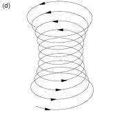
Figure 2: Paths of the fluid material elements for single-cell vortex (vortex ring) within a layer, which is also a vortex ring. (a) $r-\theta$ plane at $\lambda z=-\frac{\pi}{4}$, (b) $r-\theta$ plane at $\lambda z=\frac{\pi}{4}$, (c) the secondary circulation in $z-r$ plane, (d) the spiral path of the fluid material element within the vortex near the kernel.

In the present solution $\Psi(r,z)=R(r)\cos(\lambda z)$ has multiply layers by noting that the solution is periodic in $z$-coordinate. The fluid material elements are restricted within different vertical layers. So we call such flow as multi-planar flow. In each layer (e.g., $-\frac{\pi}{2}\leq\lambda z\leq\frac{\pi}{2}$), the flow has a similar behavior. It flows inward from the far to the axis ($-\frac{\pi}{2}\leq\lambda z\leq 0$, Fig.2a), and outward from the axis to the far ($0\leq\lambda z\leq\frac{\pi}{2}$, Fig.2b). Thus this secondary flow is a convection flow for $R(r)=r^{2}e^{-k^{2}r^{2}}$. V_r&=λsin(λz)re^-k^2r^2,
V_θ=±8k^2+λ^2 cos(λz) re^-k^2r^2-12fr,
V_z=2cos(λz)(1-k^2r^2)e^-k^2r^2.

The primary circulation (i.e., the tangent velocity $V_{\theta}$) has similar properties like these of the above solution. The three intrinsic length scales are still valid for this convection flow solution.

For the secondary circulation flow, there is a close circulation in $z-r$ plane (Fig.2c). This convection cell is like a vortex ring in fluid dynamics, so it is also vortex ring flow solution. This secondary circulation consists of radial inflow at low levels, which spirals inward toward the vortex center, then turns up out of the boundary layer and travels up along the vortex column, eventually expanding outward with height. The swirl ratio becomes,

$$S=\frac{V^{1}_{\theta m}}{V_{rm}}=\frac{\sqrt{8k^{2}+\lambda^{2}}}{\lambda\tan(\lambda z)}=\frac{\sqrt{8A_{s}^{2}+1}}{\tan(\lambda z)}$$ (10)

Thus the secondary circulation is always weaker than the primary circulation within $-\frac{\pi}{4}\leq\lambda z\leq\frac{\pi}{4}$. The spiral path of the fluid material element within the vortex near the kernel is depicted in Fig.2d. As the function $R(r)$ in Eq.(2) is the same in Eq.(1), there are also three intrinsic length $r_{m}$, $r_{k}$ and $r_{d}$, which are right the same with these in the previous solution.

Figure 3: (a) The radius and vertical velocities for double-cell vortex and (b) the corresponding secondary circulation in $z-r$ plane.

Besides, the secondary circulation could be multi-cell. In this case, the substitution of $R$ in Eq.(LABEL:Eq:Axisflow-velsol-R,gamma!=0) to the streamfunction $\Psi(r,z)=P(r)R_{0}(r)\cos(\lambda z)$ gives the multi-cell secondary circulation solutions, where $P_{2}(r)=(1-k^{2}r^{2})$ or $P_{4}(r)=(1-2k^{2}r^{2}+2/3k^{4}r^{4})$, and etc. The flow velocity is, V_r&=λsin(λz)P(r)R0(r)r,
V_θ=μP(r)R0(r)r cos(λz)-12fr,
V_z=[P(r)R0(r)]’rcos(λz). where $\mu=\sqrt{16k^{2}+\lambda^{2}}$ for $P_{2}(r)$ and $\mu=\sqrt{24k^{2}+\lambda^{2}}$ for $P_{4}(r)$. It should be noted that $\mu$ is different from that in the above solutions. As there are multi-cell circulations, there are also several local maximums for both radial velocity and tangent velocity.

For $P_{2}(r)=(1-k^{2}r^{2})$, the velocities of $V_{r}$ and $V_{z}$ are depicted in Fig.3a. The two-cell solution has a close circle, and $V_{r}$ changes sign across $r_{0}=1/k$. Thus, $r=r_{0}$ is a limit circle in primary circulation: fluid outside $r_{0}$ will move inward to $r_{0}$, while that inside $r_{0}$ will move outward to $r_{0}$ (Fig.3b). Therefore, near $r_{0}$ there must be a strong axial flow, which in turn requires an axial flow of opposite direction near $r=0$. Such vertical velocity distribution is something like that of the Sullivan vortex TongBGVortexBook2009; WuJZbook2006. Comparing the secondary circulations in Fig.3 with that in Fig.2, the size of the first circulation becomes smaller. The three intrinsic lengths are $r_{m}\approx 0.468/k$, $r_{k}\approx 0.618/k$ and $r_{d}=r_{0}=1/k$. Similarly, the swirl ratio is,

$$S=\frac{V^{1}_{\theta m}}{V_{rm}}=\frac{\sqrt{16k^{2}+\lambda^{2}}}{\lambda\tan(\lambda z)}=\frac{\sqrt{16A_{s}^{2}+1}}{\tan(\lambda z)}$$ (11)

For $P_{4}(r)=(1-2k^{2}r^{2}+2k^{4}r^{4}/3)$, the velocities of $V_{r}$ and $V_{z}$ are depicted in Fig.4a. The vertical velocity changes signs for three times. So the secondary circulation is triple-cell (Fig.4b). The intrinsic length scales in above solution do not make sense. The three intrinsic lengths are $r_{m}\approx 0.377/k$, $r_{k}\approx 0.496/k$ and $r_{d}=r_{0}\approx 0.796/k$. Similarly, the swirl ratio is,

$$S=\frac{V^{1}_{\theta m}}{V_{rm}}=\frac{\sqrt{24k^{2}+\lambda^{2}}}{\lambda\tan(\lambda z)}=\frac{\sqrt{24A_{s}^{2}+1}}{\tan(\lambda z)}$$ (12)

As calculated above, there is always $r_{0}=r_{d}$ for two-cell and triple-cell vortex solution. This can be stated as a general result (see Appendix for proof).

Theorem 2: For axisymmetric ideal incompressible flow, there is an intrinsic radius $r_{0}$. When the radius velocity vanishes at $r=r_{0}$, the vertical velocity approaches to its maximum value, and the primary vorticity approaches to its maximum value simultaneously, i.e., $r_{0}=r_{d}$.

Figure 4: (a) The radius and vertical velocities for triple-cell vortex, where $r_{m}\approx 0.377r_{s}$, $r_{k}\approx 0.496r_{s}$, $r_{w1}=r_{0}\approx 0.796r_{s}$, and $r_{w2}=r_{0}\approx 2.45r_{s}$. (b) The corresponding secondary circulation in $z-r$ plane.

In a word, this kind of solution can be multi-layer and multi-cell. There are three intrinsic length scales in the solution. One is the radius of maximum primary circular velocity $r_{m}$. The other is the radius of the vortex kernel $r_{k}>r_{m}$ for the secondary circulation, which is also the boundary of positive vorticity and negative vorticity for the primary circulation. The last one is the radius of the maximum primary vorticity $r_{d}$, at which the vertical flow of the secondary circulation approaches its maximum, and across which the radius velocity changes sign.

4 Discussion

4.1 Extensions of Solutions

In section § 2, we have mentioned that the constant $a$ could be either positive ($a=1$) or negative ($a=-1$). The different choice makes different rotation. The secondary circulation is cyclonic in $z-r$ plane for positive $a$, it is anticyclone for negative one. The anticyclonic one favors the deep convection near the eyewall, where the flow cyclonically-rotating (in $r-\theta$ plane) upward (in $z$ direction) as vortical hot tower (VHT) Hendricks2004. This may happen in the intensification of the TC. The cyclonic one suppresses the convection, which may happen in the decline of the TC. Both modes are intrinsic in the TC. It is the environment condition that determine which one should be at the certain stage of TC life.

It is also mentioned above that there are only two constants ($\mu$ and $k$) in the problem of Eq.(20) and/or Eq.(18). For any given pair of $\mu$ and $k$, there might be series of different solutions for different $\lambda$. As both equations are linear, any linear superposition of the solutions should also satisfy the equations. So we could use this linear superposition to obtain more useful solutions in applications.

An alternative way to obtain new solution is that using two different solutions combine as a new one, like the Rankine vortex. For example, we let $a\neq 0$ and $b=0$ in Eq.(Ba) as the inner solution, and let $a=0$ and $b\neq 0$ as a outer solution. The new combine one is a Rankine-like vortex with vertical stretch of $H(z)$.

According to the previous studies Batchelor1967; Frewer2007, the solution set is quite large, which can also be seen from the Eq.(1). According to Batchelor1967, the vertical velocity $V_{\theta}=C(\Psi)/r$, while we simply took the velocity components as a form $V_{\theta}=\mu\Psi/r$ in Eq.(1). Beyond present study, there should be other axisymmetric solutions. For example, we can apply the same approach to find other exact solutions by taking $V_{\theta}=\mu/r$ or $V_{\theta}=\mu\Psi^{2}(r,z)/r$, etc.

4.2 Aspect and Swirl ratios

In the subsection 3.1, we consider a single layer flow with e-fold stretching in vertical axis. The aspect radio for one-cell vortex yields to $A_{s}>\sqrt{2}/4$ for $\Psi=r^{2}e^{-\lambda z-k^{2}r^{2}}$ ($P_{0}(r)=1$ in Eq.(21) ), according to the swirl ratio in Eq.(8). This implies that the vertical scale must larger than a critical value for a given horizontal length scale. On the other hand, if the vertical scale is given, then the horizontal length scale is also bounded. For example, if the vertical length is $h_{0}$, then the standard horizontal lengthes $r_{s}$ yield to, r_s&≤22h_0, for   P_0
r_s≤4h_0, for   P_1
r_s≤42h_0, for   P_2 From above relations, a bigger vortex should contain more secondary cells. However, a bigger vortex (smaller $A_{s}$) also implies a weaker swirling flow (smaller $S$ in Eq.(10) ). In contrast to that, there is no constrain of the aspect ratio for the multi-layer flow in the subsection 3.2. Thus the vortex could be thin and flat, like a thin-film.

In both cases, the swirl ratios are approximately positive proper to the aspect radios. If the convection layer is higher, then the swirl is weaker. On the other hand, if the vertical velocity is strong, then this secondary convection layer must very thin comparing to the horizontal scale.

4.3 Possible Applications

As mentioned above, a stretch-free inviscid vortex (two-dimensional axisymmetric columnar vortex) can have arbitrary radial dependence for $H(z)=1$ WuJZbook2006. However, many well-known vortex solutions are always similar to either Eq.(Ba) or Eq.(Bb). It is from this study that these two-dimensional axisymmetric columnar vortices are also the three-dimensional axisymmetric columnar vortex solutions. So we can find either the Rankine or Taylor vortex for any fixed layer $z=const$.

As the exact solutions are finite within the whole region, they can be applied to study the radial structure of the tornados, the TCs and the mesoscale eddies in the geophysical flows. As mentioned above, there are 3 independent parameters in the solution. To determinate them, we need the measurable qualities, such as the radius of circular velocity maximum $r_{m}$, the maximum circular velocity $V_{\theta m}$, the spiral angle defined by $\lambda/\mu$, the angular momentum $m$, etc. According to Eq.(1), the angular momentum $m=rV_{\theta}=-\mu R(r)H(z)$, thus the solutions of $R(r)$ (Eq.(LABEL:Eq:Axisflow-velsol-R,gamma!=0) and Eq.(B)) can be applied to discuss the angular momentum of the vortex. For the tornado and TC observations, such solutions can be used to fit the real velocity distribution along the radial coordinate. This may also be useful to classify the tornados and the TCs according the flow structures provided by above solutions.

It is from Eq.(8) that the vertical flow could be either weak (in whole height) or strong (only in boundaries) for universal inflow solution. While from Eq.(10), the vertical flow could be either weak (in the middle height of the region) or strong (only near the boundaries). It seems that the relative strong radius velocity could be easily found near boundaries.

An alternative application is the bogus TC in numerical simulations. These new solutions have vertical velocity, which could enhance the boundary inflow in a three-dimensionally nonhydrostatic model.

5 Conclusion

This investigation solve the three-dimensional ideal model to obtain the TC-like vortex solution with a secondary circulation. We prove two Theorems for axisymmetrically incompressible ideal flow. First, there is an intrinsic radius $r_{k}$, within which is the kernel of the primary vortex. The vortex boundary $r_{k}$ is the frontier of the positive and negative vorticity of the primary circulation, and also the frontier of upward and downward flows of the secondary circulation. The maximum velocity of the primary circulation locates within the vortex kernel, i.e., the radius of maximum wind (RMW in TC studies, namely $r_{m}$) $r_{m}<r_{k}$. Second, there is an intrinsic radius $r_{0}$. When the radius velocity vanishes at $r=r_{0}$, the vertical velocity approaches to its maximum value, and the maximum primary vorticity approaches to its maximum value simultaneously, i.e., $r_{0}=r_{d}$. It seems that the relative stronger radius velocity could be easily found near boundaries.

The explicit TC-like vortex and multi-layer vortex solutions, which are new in this investigation, might be used to describe the 3D structure of the tropical cyclones, tornados and mesoscale eddies in the geophysical flows. The solutions can also be applied as bogus TCs in numerical simulations.

The method used in present work is very straightforward, and it could also be applied to other complex flows, and even for the non-steady viscous flows like Kieu2009 tried.

The author thanks Prof. Wang W. at OUC, who discussed lots of vortex dynamic problems with the author and encouraged the author to finish this work. The author also thanks Dr. Wang Bo-fu and Dr. Wan Zhen-hua for their help to check the formula, Prof. Huang Rui-Xin at WHOI for useful comments. Prof. Yin X-Y at USTC is also acknowledged, who led the author to this field. This work is supported by the National Basic Research Program of China (No. 2012CB417402 and 2013CB430303), the National Foundation of Natural Science (Nos. 41376017), and the Open Fund of State Key Laboratory of Satellite Ocean Environment Dynamics (No. SOED1209).

Appendix A Proofs

We first prove the Theorem 1 from Eq.(2) with $f=0$ without loss of universality. According to Eq.(2a), the vertical velocity of the secondary circulation is $V_{z}=-\frac{1}{r}\frac{\partial\Psi}{\partial r}$. Integrating Eq.(2b) with $f=0$ gives a first integral for the momentum $M$. As $M(\Psi)$ is a function only $\Psi$ belong, the vorticity of the primary circulation is,

$$\omega=\frac{1}{r}\frac{\partial M}{\partial r}=\frac{M^{\prime}}{r}\frac{\partial\Psi}{\partial r}=-M^{\prime}V_{z}.$$ (13)

When the vertical velocity $V_{z}=0$ (i.e. $\frac{\partial\Psi}{\partial r}=0$) at a certain radius $r_{k}$, the vorticity $\omega=0$ simultaneously. This is the proof of the first part of the Theorem 1. According to the integration, the azimuth velocity is $V_{\theta}=\frac{1}{r}M(\Psi)$. So the first deviation of $V_{\theta}$ to $r$ is,

$$V^{\prime}_{\theta}=\frac{\partial}{\partial r}(\frac{M}{r})=\frac{M^{\prime}}{r}\frac{\partial\Psi}{\partial r}-\frac{1}{r}\frac{M}{r}=\omega-\frac{V_{\theta}}{r}.$$ (14)

At $r=r_{k}$, it becomes $V^{\prime}_{\theta}(r_{k})=-V_{\theta}(r_{k})/r_{k}$ for $\omega=0$. The value of $V_{\theta}(r_{k})$ could be calculated by integrating

$$V_{\theta}(r_{k})=\int_{0}^{r_{k}}V^{\prime}_{\theta}(r)dr=r_{k}V^{\prime}_{\theta}(r_{s})$$ (15)

where $0<r_{s}<r_{k}$. Substituting the above result to $V^{\prime}_{\theta}(r_{k})$, it yields $V^{\prime}_{\theta}(r_{k})=-V^{\prime}_{\theta}(r_{s})$. So there must be a radius $r_{m}$ within $[r_{s},r_{k}]$, where $V^{\prime}_{\theta}(r_{m})=0$. So we proved the second part of the Theorem 1.

Then we solve the system of Eq.(2). Substituting Eq.(1) into Equation (2c) and equation (2d) becomes, (Rr)(Rr)’H’^2 - (Rr)(R’r)HH”-μ2r3R^2H^2 =-1ρ∂p∂r
(R’r)^2 HH’ - (Rr)(R’r)’ HH’ = -1ρ∂p∂z Hence, the pressure can be solved from Eq.(4),

$$p(r,z)=E-\frac{\rho}{2}V^{2}=\frac{\rho}{2}(4k^{4}R^{2}H^{2}-\frac{\mu^{2}R^{2}}{r^{2}}H^{2}-\frac{R^{2}}{r^{2}}H^{\prime 2}-\frac{R^{\prime 2}}{r^{2}}H^{2})$$ (16)

Substituting Eq.(16) into Eq.(Aa) and Eq.(Ab), both yield

$$(R^{\prime\prime}-\frac{R^{\prime}}{r}+\mu^{2}R-4k^{4}r^{2}R)H+RH^{\prime\prime}=0$$ (17)

The above equation is a special case of Bragg-Hawthorne equation Batchelor1967; Frewer2007,

$$\Psi_{zz}+\Psi_{rr}-\frac{1}{r}\Psi_{r}=r^{2}G(\Psi)+F(\Psi)$$ (18)

Here both $F=-\mu^{2}\Psi$ and $G=4k^{4}\Psi$ are linear functions of $\Psi$, although $F$ and $G$ could be nonlinear in general Batchelor1967; Frewer2007.

Recall that $R$ and $H$ are independent, we can solve the above equation. There are three kind of functions for $H(z)$ in Eq.(17). The first trivial one is $H=1$, any differentiable function $R(r)$ would be the solution, e.g. the Rankine vortex Mallen2005; SunL2011arx. The second one is $H(z)=z$, one can obtains the Sullivan vortex WuJZbook2006 and other vortex solutions SunL2011arx. Third, it also yields two kind of non-trivial solutions for $H(z)$,

$$H(z)=e^{-\lambda(z-z_{0})}\,\,or,\,\,H(z)=\cos(\lambda(z-z_{0})).$$ (19)

where $z_{0}$ is a constant parameter. We simply take $z_{0}=0$ in the following investigation. Substitution Eq.(19) into Eq.(17) to eliminate the function for $z$ (plus for $H(z)=e^{\lambda z}$ and minus for $H(z)=\cos(\lambda z)$, respectively), it yields to

$$R^{\prime\prime}-\frac{R^{\prime}}{r}+(\mu^{2}\pm\lambda^{2})R-4k^{4}r^{2}R=0$$ (20)

It is obvious that $\lambda=0$ reduces to the second case of $H(z)=z$. Before solving the equation, we prove the Theorem 2. It is from Eq.(17) or the above equation that $R=0$ implies $R^{\prime\prime}r=R^{\prime}$. Applying the velocity solution in Eq.(1), when $V_{r}=0$ at $r=r_{0}$, then $\partial(V_{z})/\partial r=0$. This implies that when the radius velocity vanishes at $r=r_{0}$, the vertical velocity approaches to its maximum value. According to Eq.(13), the primary circulation vorticity approaches to its maximum value simultaneously. So we proved the Theorem 2.

Appendix B Solution

Then we solve the above Equation (20). When $\mu^{2}\pm\lambda^{2}=0$, Eq.(20) has the solutions of R(r) &= ar^2-b, for   k^2=0,
R(r) = ae^-k^2r^2, for   k^2≠0 When the energy $E$ is homogeneous ($k=0$), the solution of Eq.(Ba) is the Rankine vortex WuJZbook2006. The solution of Eq.(Bb) is the Oseen vortex WuJZbook2006. Let $R=r^{2}e^{-k^{2}r^{2}}P(r)$, Eq.(20) yields

$$r^{2}P^{\prime\prime}+(3r-4k^{2}r^{3})P^{\prime}+(\mu^{2}\pm\lambda^{2}-8k^{2})P=0$$ (21)

And there are some polynomial solutions of $P(r)$, P_0(r) &= 1,   μ^2±λ^2-8k^2=0
P_2(r) = 1-k^2r^2,   μ^2±λ^2-8k^2=8k^2
P_4(r) = 1-2k^2r^2+23k^4r^4,   μ^2±λ^2-8k^2=16k^2 The solution of Eq. (20) for yields, R_0(r) &= r^2e^-k^2r^2 ,   μ^2±λ^2-8k^2=0
R_2(r) = (1-k^2r^2)r^2e^-k^2r^2,   μ^2±λ^2-8k^2=8k