Abstract

We present an analysis of nonperturbative contributions to the transverse momentum distribution of $Z/\gamma^{*}$ bosons produced at hadron colliders. The new data on the angular distribution $\phi^{*}_{\eta}$ of Drell-Yan pairs measured at the Tevatron is shown to be in excellent agreement with a perturbative QCD prediction based on the Collins-Soper-Sterman (CSS) resummation formalism at NNLL accuracy. Using these data, we determine the nonperturbative component of the CSS resummed cross section and estimate its dependence on arbitrary resummation scales and other factors. With the scale dependence included at the NNLL level, a significant nonperturbative component is needed to describe the angular data.

1 Introduction

QCD factorization methods utilizing transverse-momentum-dependent (TMD) parton distributions and fragmentation functions provide a powerful framework for describing multi-scale observables in high-energy hadron interactions. Production of Drell-Yan lepton-antilepton pairs in $Z/\gamma^{*}$ boson production in hadron-hadron collisions is one basic process in which TMD factorization is applied to predict the boson’s transverse momentum ($Q_{T}$) distribution and related angular distributions. Collinear QCD factorization is applicable for describing lepton pairs with $Q_{T}$ of order of the invariant mass $Q$ of the pair. The respective large-$Q_{T}$ cross sections have been computed up to two loops in the QCD coupling strength $\alpha_{s}$ [1, 2, 3, 4] and are in reasonable agreement with the data.

But, at small $Q_{T}$, all-order resummation of large logarithms $\ln(Q_{T}/Q)$ needs to be performed [5, 6, 7] to obtain sensible cross sections. TMD factorization provides a systematic framework for $Q_{T}$ resummation to all orders in $\alpha_{s}$, as has been shown in classical papers by Collins, Soper, and Sterman (CSS) [8, 9, 10, 11, 12]. The resummed cross sections have been computed at various QCD orders in the CSS formalism and kindred approaches  [13, 14, 15, 16, 17, 18, 19, 3, 4, 20, 21, 22]. In addition to perturbative radiative contributions, the resummed cross sections include a nonperturbative component associated with QCD dynamics at momentum scales below 1 GeV. Understanding of the nonperturbative terms is important for tests of TMD factorization and precision studies of electroweak boson production, including the measurement of $W$ boson mass [23].

Instead of measuring $Q_{T}$ distributions directly, one can measure the distribution in the angle $\phi^{*}_{\eta}$ [24] that is closely related to $Q_{T}/Q$. The $\phi^{*}_{\eta}$ distributions have been recently measured both at the Tevatron [25] and Large Hadron Collider [26, 27]. Small experimental errors of the $\phi^{*}_{\eta}$ measurements (as low as 0.5%) allow one to test the $Q_{T}$ resummation formalism at an unprecedented level. On the theory side, the small-$Q_{T}$ resummed form factor for $Z$ boson production has been computed to NNLL/NNLO [28]. We would like to confront precise theoretical predictions implemented in programs Legacy and ResBos [29, 30, 31] by the new experimental data to obtain quantitative constraints on the nonperturbative contributions.

Such analysis is technically challenging and requires to examine several effects that were negligible in the previous studies of the resummed nonperturbative terms [29, 31, 32]. The framework for the fitting of Drell-Yan processes in the CSS formalism must be extended to the $\phi^{*}_{\eta}$, rather than $Q_{T}$, distributions. Nonperturbative effects must be distinguished from comparable modifications by NNLO QCD corrections, NLO electroweak (EW) corrections, and the associated perturbative uncertainties.

To carry out this study, we modified the $Q_{T}$ resummation calculation employed in our previous studies to evaluate NNLO QCD ($\alpha_{s}^{2}$) and NLO EW ($\alpha_{EW}$) perturbative contributions and consider the residual QCD scale dependence associated with higher-order terms. This implementation was utilized to determine the nonperturbative factor from the DØ Run-2 data on the $\phi^{*}_{\eta}$ distributions.

Our findings shed light on several questions raised in recent studies of TMD factorization [33, 34, 35, 36, 37, 38, 39, 40, 41, 42, 43, 44, 45] and soft-collinear-effective (SCET) theory [46, 47, 48]. We examine if the $\phi^{*}_{\eta}$ data corroborate the universal behavior of the resummed nonperturbative terms that is expected from the TMD factorization theorem [11] and was observed in the global analyses of Drell-Yan $Q_{T}$ distributions at fixed-target and collider energies [31, 32]. We also investigate the rapidity dependence of the nonperturbative terms, which may be indicative of new types of higher-order contributions [49]. It has been argued [4, 50, 20, 21, 22] that the evidence for nonperturbative smearing is inconclusive because of a large QCD scale dependence. Since the magnitude of the scale dependence reduces with the order of the calculation, we include the dependence on the soft scales in the resummed cross section up to ${\cal O}(\alpha_{s}^{2})$, i.e. NNLL/NNLO. In this case, the radiative contributions are estimated to the same order as in [28], either exactly or approximately, and we also include contributions responsible for the dependence on the resummation scales to one higher order ($\alpha_{s}^{2}$) than in [4, 50, 20, 21, 22].

Based on our numerical implementation, we demonstrate that the impact of the power-suppressed contributions is generically distinct from the scale dependence: the nonperturbative effects can be distinguished from the NNLO scale uncertainties. The nonperturbative component that we find is consistent with a universal quadratic (Gaussian) power-suppressed contribution of the kind that may be expected on general grounds [11], and of a magnitude that is compatible with a previous global analysis of Drell-Yan $Q_{T}$ distributions [32].

The DØ data are precise enough and may be able to distinguish between the Gaussian and alternative nonperturbative functions that have been recently proposed [51]. It would be insightful to examine constraints on a variety of the nonperturbative models that are currently discussed [45, 46, 44, 52], as well as the $\sqrt{s}$ dependence of the nonperturbative contributions by using a combination of the Tevatron and LHC data. As such investigation demands significant computational resources, it will be pursued in future work.

Our main numerical results have been reported at the QCD Evolution Workshop at Thomas Jefferson National Accelerator Facility in May 2012 [53]. The current paper documents this analysis in detail and is organized as follows. Section 2 reviews the relation between the $\phi_{\eta}^{*}$ angle and transverse momentum $Q_{T}$ in the Collins-Soper-Sterman notations (Sec. 2.1), general structure of the resummed cross section and estimation of NNLO contributions and their scale dependence (Secs. 2.2, 2.3, 2.4), nonperturbative model (Sec. 2.5), matching of the small-$Q_{T}$ and large-$Q_{T}$ terms (Sec. 2.6), photon radiation contribution (Sec. 2.7), and numerical accuracy (Sec. 2.8). In Sec. 2.9, distinctions between the NNLL/NNLO resummed $Q_{T}$ distributions obtained in the CSS formalism and the alternative approach of Refs. [82, 19, 28] are summarized.

Next, in Sec. 3, the size of the nonperturbative contributions is estimated by a $\chi^{2}$ analysis of the DØ data in three bins of vector boson rapidity ($y_{Z}$), by applying two different methods to examine the scale dependence of the resummed cross section. By using the constraining power of this data set, we suggest a Gaussian smearing factor suitable for $W$ and $Z$ production, and we give an estimate at 68% C.L. for the leading parameter of the NP functional form. We provide the user with several sets of grids of theory predictions for phenomenological applications based on CT10 NNLO [54] PDF eigenvector sets, and for scans of the nonperturbative smearing function and estimates of its uncertainty in future measurements.

2 Overview of the resummation method

2.1 Relation between $Q_{T}$ and $\phi^{*}_{\eta}$ variables

The Collins-Soper-Sterman (CSS) resummation formalism predicts fully differential distributions in electroweak boson production, including decay of heavy bosons. While the original formulation of the CSS formalism deals with resummation of logarithms dependent on the boson’s transverse momentum $Q_{T}$, it can be readily extended to resum angular variables of decay particles. One such variable is the azimuthal angle separation $\Delta\varphi$ of the leptons in the lab frame, which approaches $\pi$ (back-to-back production of leptons in the transverse plane) when $Q_{T}\rightarrow 0$. Consequently, the region $\Delta\varphi\rightarrow\pi$ is sensitive to small-$Q_{T}$ resummation [30].

Recently, an angular variable $\phi_{\eta}^{*}$ was proposed in [24] that has an experimental advantage compared to $Q_{T}$ and $\Delta\varphi$. The $\phi_{\eta}^{*}$ variable is not affected by the experimental resolution on the magnitudes of the leptons’ (transverse) momenta that limits the accuracy of the $Q_{T}$ measurement. Soft and collinear resummation for the $\phi^{*}_{\eta}$ distribution can be worked out either analytically [20, 21, 50, 22] or numerically by integrating the resummed $Q_{T}$ distribution over the leptons’ phase space.

To describe decays of massive bosons, the CSS formalism [30] usually operates with the lepton polar angle $\theta_{CS}$ and azimuthal angle $\varphi_{CS}$ in the Collins-Soper (CS) reference frame [55]. The CS frame is a rest frame of the vector boson in which the $z$ axis bisects the angle formed by the momenta $\vec{p}_{1}$ and -$\vec{p}_{2}$ of the incident quark and antiquark. In the CS frame, the decay leptons escape back-to-back ($\vec{l}_{1}+\vec{l}_{2}=0$), and the electron’s and positron’s 4-momenta are

$$\left.l_{1}^{\mu}\right|_{\mbox{CS frame}}=(Q/2)\left\{1,\cos\varphi_{CS}\sin\theta_{CS},\sin\varphi_{CS}\sin\theta_{CS},\cos\theta_{CS}\right\},$$ (1)

and

$$\left.l_{2}^{\mu}\right|_{\mbox{CS frame}}=(Q/2)\left\{1,-\cos\varphi_{CS}\sin\theta_{CS},-\sin\varphi_{CS}\sin\theta_{CS},-\cos\theta_{CS}\right\}.$$ (2)

On the other hand, the angular variable $\phi_{\eta}^{*}$ is defined in a different frame (“$\eta$ frame”), in which the leptons escape $\theta_{\eta}^{*}$ and $\pi-\theta_{\eta}^{*}$ with respect to the incident beams direction. The $\eta$ frame is related to the lab frame by a boost $\beta=\tanh(\left(\eta_{1}+\eta_{2}\right)/2)$ along the incident beam direction, where $\eta_{1}$ and $\eta_{2}$ are the pseudorapidities of $e^{-}$ and $e^{+}$ in the lab frame. The frame coincides with the CS frame when $Q_{T}=0$. Knowing the polar angle $\theta_{\eta}^{*}$ in the $\eta$ frame and the difference $\Delta\varphi=\varphi_{1}-\varphi_{2}$ of the lepton’s azimuthal angles in the transverse plane to the beam direction, one defines

$$\phi^{*}_{\eta}=\tan{\left(\phi_{acop}/2\right)}\sin{\theta^{*}_{\eta}}$$ (3)

in terms of the acoplanarity angle $\phi_{acop}=\pi-\Delta\varphi$. We write $\cos\theta_{\eta}^{*}$ as a function of the lepton momenta in the lab frame as

$$\cos\theta^{*}_{\eta}=\tanh\left(\frac{\eta_{1}-\eta_{2}}{2}\right)=\frac{\sqrt{l^{+}_{1}l_{2}^{-}}-\sqrt{l^{-}_{1}l^{+}_{2}}}{\sqrt{l^{+}_{1}l_{2}^{-}}+\sqrt{l^{-}_{1}l^{+}_{2}}}=\frac{f\left(\cos\theta_{CS}\right)-f\left(-\cos\theta_{CS}\right)}{f\left(\cos\theta_{CS}\right)+f\left(-\cos\theta_{CS}\right)},$$ (4)

where $l^{\pm}_{1,2}=(l^{0}_{1,2}\pm l^{z}_{1,2})/\sqrt{2}$,

$$f(\cos\theta_{CS})\equiv\sqrt{M_{T}^{2}+2M_{T}Q\cos\theta_{CS}+Q^{2}\cos^{2}\theta_{CS}-Q_{T}^{2}\sin^{2}\theta_{CS}\cos^{2}\varphi_{CS}},$$ (5)

and $M_{T}^{2}=Q^{2}+Q_{T}^{2}$. We also write $\cos{\Delta\varphi}$ as

$$\cos{\Delta\varphi}=(Q_{T}^{2}-Q^{2}\sin^{2}\theta_{CS}-Q_{T}^{2}\sin^{2}\theta_{CS}\cos^{2}\varphi_{CS})$$

$$\times[(Q^{2}\sin^{2}\theta_{CS}+Q_{T}^{2}\sin^{2}\theta_{CS}\cos^{2}\varphi_{CS}+Q_{T}^{2})^{2}-4M_{T}^{2}Q_{T}^{2}\sin^{2}\theta_{CS}\cos^{2}\varphi_{CS}]^{-\frac{1}{2}}.$$ (6)

In the limit $Q_{T}\rightarrow 0$, $\phi^{*}_{\eta}$ simplifies to

$$\phi^{*}_{\eta}\approx(Q_{T}/Q)\sin\varphi_{CS},$$ (7)

since $\tan(\phi_{acop}/2)=\sqrt{\left(1+\cos\Delta\varphi\right)/\left(1-\cos\Delta\varphi\right)}$, and

$$\theta^{*}_{\eta}\rightarrow\theta_{CS}, \cos{\Delta\varphi}\rightarrow-1+2\left(\frac{Q_{T}}{Q}\frac{\sin\varphi_{CS}}{\sin\theta_{CS}}\right)^{2}.$$ (8)

Measurement of $\phi^{*}_{\eta}$ thus directly probes $Q_{T}/Q$.

Relations like these can analytically express the $\phi^{*}_{\eta}$ distribution in terms of the $Q_{T}$ distribution, but in practice it is easier to compute the $\phi^{*}_{\eta}$ distribution by Monte-Carlo integration in ResBos code. In this case, the interval of small $Q_{T}/Q$ maps onto the region of small $\phi^{*}_{\eta}$. For example, in $Z$ production at $Q\approx M_{Z}$, the range $10^{-3}\leq\phi^{*}_{\eta}\leq 0.5$ radians corresponds to $0.1\lesssim Q_{T}\lesssim 50$ GeV.

2.2 General structure of the resummed cross section

The resummed cross sections that we present are based on the calculation in [13, 29, 30, 31] with added higher-order radiative contributions (Secs. 2.3, 2.4) and modified nonperturbative model (Sec. 2.5). We write the fully differential cross section for $Z$ boson production and decay as

$$\frac{d\sigma\left(h_{1}h_{2}\rightarrow(Z\rightarrow\ell\bar{\ell})X\right)}{dQ^{2}\ dy_{Z}\ dQ_{T}^{2}\ d\cos\theta_{CS}\ d\varphi_{CS}}=\sum_{\alpha=-1}^{4}F_{\alpha}\left(Q,Q_{T},y\right)A_{\alpha}\left(\theta_{CS},\varphi_{CS}\right)$$ (9)

in terms of the structure functions $F_{\alpha}(Q,Q_{T},y_{Z})$ and angular functions $A_{\alpha}(\theta_{CS},\varphi_{CS})$. The variables $Q$, $Q_{T}$, and $y_{Z}$ correspond to the invariant mass, transverse momentum, and rapidity of the boson in the lab frame; $\theta_{CS}$ and $\varphi_{CS}$ are the lepton decay angles in the CS frame. Among the structure functions $F_{\alpha}$, two (associated with the angular functions $A_{-1}=1+\cos^{2}\theta_{CS}$ and $A_{3}=2\cos\theta_{CS}$) include resummation of soft and collinear logarithms in the small-$Q_{T}$ limit. For such functions, we write

$$F_{\alpha}(Q,Q_{T},y_{Z})=W_{\alpha}(Q,Q_{T},y_{Z};C_{1}/b,C_{2}Q,C_{3}/b)+Y_{\alpha}(Q,Q_{T},y_{Z};C_{4}Q),$$ (10)

where

$$W_{\alpha}(Q,Q_{T},y_{Z})=\int\frac{d^{2}b}{4\pi^{2}}\,e^{i\vec{Q}_{T}\cdot\vec{b}}\sum_{j=u,d,s...}\widetilde{W}_{\alpha,j}(b,Q,y_{Z})$$ (11)

is introduced to resum small-$Q_{T}$ logarithms to all orders in $\alpha_{s}$. The $W$ term depends on several auxiliary QCD scales $C_{1}/b$, $C_{2}Q$, and $C_{3}/b$ with constant coefficients $C_{1,2,3}\approx 1$ that emerge from the solution of differential equations describing renormalization and gauge invariance of $Q_{T}$ distributions [8, 12]. $Y_{\alpha}(Q,Q_{T},y_{Z};C_{4}Q)$ is a part of the non-singular remainder, or “the $Y$ term”’. It depends on a factorization and renormalization momentum scale $C_{4}Q$.

The Fourier-Bessel integral over the transverse position $b$ in the $W$ term in Eq. (11) acquires contributions from the region of small transverse positions $0\leq b\lesssim 1\mbox{ GeV}^{-1}$, where the form factor can be approximated in perturbative QCD, and the region $b\gtrsim 1\mbox{ GeV}^{-1}$, where the perturbative expansion in the QCD coupling $\alpha_{s}(1/b)$ breaks down, and nonperturbative methods are necessitated. In $Z$ boson production, the small-$b$ perturbative contribution dominates the Fourier-Bessel integral for any $Q_{T}$ value [7, 32, 57]. At $Q_{T}$ below 5 GeV, the production rate is also mildly sensitive to the behavior in the $b>0.5$ GeV^-1 interval, where the full expression for $\widetilde{W}_{\alpha,j}(b,Q)$ is yet unknown.

To determine the acceptable large-$b$ forms of $\widetilde{W}_{\alpha,j}(b,Q)$ by comparison to the latest $Z$ boson data, we need to update the leading-power contribution to $\widetilde{W}_{\alpha,j}(b,Q,y_{Z})$ computable in perturbative QCD, denoted by $\widetilde{W}_{\alpha,j}^{pert}(b,Q,y_{Z})$, by considering additional QCD and electromagnetic corrections and dependence on QCD factorization scales. In particular, scale dependence in the perturbative form factor $\widetilde{W}^{pert}$ may smear the sensitivity to the nonperturbative factor [3, 20, 28, 50]. We will review the perturbative contributions in the next two subsections.

2.3 Perturbative coefficients for canonical scales

For a particular “canonical” combination of the scale parameters, the perturbative contributions simplify; the resummed form factor at $b\ll 1\mbox{ GeV}^{-1}$ takes the form

$$\widetilde{W}^{pert}_{\alpha,j}(b,Q,y_{Z}) = \sum_{j=u,d,s...}\left|H_{\alpha,j}(Q,\Omega)\right|^{2}\,\exp\left[-S(b,Q)\right]$$ (12)

$$\times \sum_{a=g,q,\bar{q}}\left[{\cal C}_{ja}\otimes f_{a/h_{1}}\right]\left(\chi_{1},\mu_{F}\right)\sum_{b=g,q,\bar{q}}\left[{\cal C}_{\bar{j}b}\otimes f_{b/h_{2}}\right]\left(\chi_{2},\mu_{F}\right)$$

in terms of a $2\rightarrow 2$ hard part $|H_{\alpha,j}(Q,\Omega)|^{2}$, Sudakov integral

$$S(b,Q)=\int_{b_{0}^{2}/b^{2}}^{Q^{2}}\frac{d\bar{\mu}^{2}}{\bar{\mu}^{2}}\left[A(\bar{\mu})\,\ln\left(\frac{Q^{2}}{\bar{\mu}^{2}}\right)+B(\bar{\mu})\right],$$ (13)

and convolutions $\left[{\cal C}_{j/a}\otimes f_{a/h}\right]$ of Wilson coefficient functions ${\cal C}_{j/a}$ and PDFs $f_{a/h}$ for a parton $a$ inside the initial-state hadron $h$. The convolution integral is defined by

$$\left[{\cal C}_{ja}\otimes f_{a/h}\right](\chi,\mu_{F})=\int_{x}^{1}\frac{d\xi}{\xi}{\cal C}_{ja}\left(\frac{\chi}{\xi},\mu_{F}\right)f_{a/h}(\xi,\mu_{F}).$$ (14)

In Eq. (14) the convolution depends on the momentum fractions $\chi_{1,2}$ that reduce to $x_{1,2}^{(0)}\equiv(Q/\sqrt{s})e^{\pm y_{Z}}$ in the limit $Q_{T}^{2}/Q^{2}\rightarrow 0$, as explained in Sec. 2.6, as well as on the factorization scale $\mu_{F}=b_{0}/b$. Some scales are proportional to the constant $b_{0}=2e^{-\gamma_{E}}=1.123...$, where $\gamma_{E}=0.577...$ is the Euler-Mascheroni constant.

The functions $H_{\alpha,j}$, $A$, $B$, and $C$ can be expanded as a series in the QCD coupling strength,

$$H_{\alpha,j}(Q,\Omega;\alpha_{s}(\bar{\mu}))=1+\sum_{n=1}^{\infty}\left(\frac{\alpha_{s}(\bar{\mu})}{\pi}\right)^{n}H^{(n)}_{\alpha,j}(Q,\Omega)\,,\quad\quad A(\alpha_{s}(\bar{\mu}))=\sum_{n=1}^{\infty}\left(\frac{\alpha_{s}(\bar{\mu})}{\pi}\right)^{n}A^{(n)}\,,\mbox{etc.}$$ (15)

Some perturbative contributions can be moved between the hard function $H_{\alpha,j}$ and Sudakov exponential depending on the resummation scheme [16]. In the Collins-Soper-Sterman (CSS) resummation scheme, $H_{\alpha,j}(\alpha_{s})=1$ to all $\alpha_{s}$ orders. In the Catani-De Florian-Grazzini (CFG) resummation scheme, $H_{\alpha,j}(\alpha_{s})$ includes hard virtual contributions starting at ${\cal O}(\alpha_{s})$, while the Sudakov exponential depends only on the type of the initial-state particle (quark or gluon) that radiates soft emissions. In Drell-Yan production, differences between the CSS and CFG schemes are small, below 1% in the kinematic region explored. We carry out the analysis in the CSS scheme, but the nonperturbative function that we obtain can be readily used with the CFG scheme.

The functions $A$ and $B$ for the canonical choice of scales are evaluated up to ${\cal O}(\alpha_{s}^{3})$ and ${\cal O}(\alpha_{s}^{2})$ respectively, using their known perturbative coefficients [58, 59, 60, 61, 62, 63]. The three-loop coefficient $A^{(3)}$ is included, but has a weak effect on the cross section (3% at $Q_{T}\approx 2$ GeV). The coefficient $A^{(3)}$ has been derived within the soft-collinear effective theory [64] and found to contain a term arising from the “collinear anomaly”, besides the ${\cal O}(\alpha_{s}^{3})$ cusp contribution known from [63]. The “collinear” anomaly contribution breaks the symmetry of the SCET Lagrangian by regulators of loop integrals [64, 65, 66, 67]. The expansion of $\widetilde{W}^{pert}$ in the CSS scheme, is found to be in agreement with that derived in SCET up to NLO. We checked that $A^{(3)}_{SCET}$ has inappreciable influence on the conclusions.

The Wilson coefficient functions ${\cal C}^{(i)}$ are computed exactly up to ${{\cal O}(\alpha_{s})}$ and approximately to ${\cal O}(\alpha_{s}^{2})$. Most of our numerical results were obtained with the ${\cal O}(\alpha_{s}^{2})$ approximation for the Wilson coefficient before the exact ${\cal O}(\alpha_{s}^{2})$ result were published [4, 3, 28]. This expression is constructed by using a numerical approximation for the canonical part of the Wilson coefficient at ${\cal O}(\alpha_{s}^{2})$ and exact expression for its dependence on soft scales. Our a posteriori comparison shows the approximation to be close to the exact expression, cf. the next subsection.

The $Y$ contribution in Eq. (11) is defined as the difference between the fixed-order perturbative $Q_{T}$ distribution calculation and the asymptotic distribution obtained by expanding the perturbative part $\widetilde{W}^{pert}$ up to the same order. It is given by

$$Y_{\alpha}(Q_{T},Q,y_{Z})=\int\frac{d\xi_{1}}{\xi_{1}}\int\frac{d\xi_{2}}{\xi_{2}}\sum_{n=1}^{\infty}\left[\frac{\alpha_{s}(C_{4}Q)}{\pi}\right]^{n}\times$$

$$f_{a/h_{1}}(\xi_{1},C_{4}Q)~{}R_{\alpha,ab}^{(n)}\left(Q_{T},Q,y_{Z};\xi_{1},\xi_{2},C_{4}Q\right)~{}f_{b/h_{2}}(\xi_{2},C_{4}Q),$$ (16)

where the functions $R_{\alpha,ab}^{(n)}$ are integrable when $Q_{T}\rightarrow 0$, and their explicit expressions for all contributing $\alpha$ to ${\cal O}(\alpha_{s})$ can be found in [10, 30]. The $O(\alpha_{s}^{2})$ contribution to the dominant structure function $Y_{-1}$ is included using the calculation in [1, 57]. $O(\alpha_{s}^{2})$ corrections to the other structure functions in the $Y$ term are essentially negligible in the small-$Q_{T}$ region of our fit.

2.4 Perturbative coefficients for arbitrary scales

The resummed form factor in Eq. (12) can be generalized to allow variations in the arbitrary factorization scales arising in the solution of Collins-Soper differential equations. At small $b$, the scale-dependent expression takes the form

$$\widetilde{W}^{pert}_{\alpha,j} = \sum_{j=u,d,s...}\left|H_{\alpha,j}(Q,\Omega,C_{2}Q)\right|^{2}\,\exp\left[-\int_{C_{1}^{2}/b^{2}}^{C_{2}^{2}Q^{2}}\frac{d\bar{\mu}^{2}}{\bar{\mu}^{2}}A(\bar{\mu};C_{1})\,\ln\left(\frac{C_{2}^{2}Q^{2}}{\bar{\mu}^{2}}\right)+B(\bar{\mu};C_{1},C_{2})\right]$$ (17)

$$\times \sum_{a=g,q,\bar{q}}\left[{\cal C}_{ja}\otimes f_{a/h_{1}}\right]\left(\chi_{1},\frac{C_{1}}{C_{2}},\frac{C_{3}}{b}\right)\sum_{b=g,q,\bar{q}}\left[{\cal C}_{\bar{j}b}\otimes f_{b/h_{2}}\right]\left(\chi_{2},\frac{C_{1}}{C_{2}},\frac{C_{3}}{b}\right),$$

where the coefficients $C_{1}=b\bar{\mu}$ and $C_{2}=\bar{\mu}/Q$ are associated with the lower and upper integration limits in Eq. (17), while $\mu_{F}=C_{3}/b$ is the factorization scale at which Wilson coefficient functions are evaluated. The “canonical” representation adopted in Eq. (12) corresponds to $C_{1}=C_{3}=b_{0}$ and $C_{2}=1$. For the rest of the discussion, we use the same scale $C_{2}Q$ to compute the hard function $H_{\alpha,j}$ and the $Y$ term, i.e. set $C_{4}=C_{2}$.

The perturbative coefficients $A^{(n)}$, $B^{(n)}$, and $C^{(n)}$ are generally dependent on the scale coefficients, but the full form factor $\widetilde{W}^{pert}$ is independent when expanded to a fixed order in $\alpha_{s}$. We can therefore reconstruct the perturbative coefficients order-by-order for arbitrary $C_{1}$, $C_{2}$, $C_{3}$ if we know the canonical values of the coefficients, indicated by the superscript “(c)”.

By truncating the series at ${\cal O}(\alpha_{s}^{2})$, we must have

$$\widetilde{W}(b,Q,C_{1},C_{2},C_{3})|_{{\cal O}(\alpha_{s}^{2})}=\widetilde{W}(b,Q,C_{1}=C_{3}=b_{0},C_{2}=1)|_{{\cal O}(\alpha_{s}^{2})}.$$ (18)

Making a series expansion on both sides of Eq. (18), we find the following relations by equating the coefficients in front of each power of $\log\left(b^{2}Q^{2}\right)$:

$$A^{(1)}(C_{1}) = A^{(1,c)};$$ (19)

$$A^{(2)}(C_{1}) = A^{(2,c)}-A^{(1,c)}\beta_{0}\ln\frac{b_{0}}{C_{1}};$$ (20)

$$A^{(3)}(C_{1}) = A^{(3,c)}-2A^{(2,c)}\beta_{0}\ln\frac{b_{0}}{C_{1}}-\frac{A^{(1,c)}}{2}\beta_{1}\ln\frac{b_{0}}{C_{1}}+A^{(1,c)}\beta_{0}^{2}\left(\ln\frac{b_{0}}{C_{1}}\right)^{2};$$ (21)

$$B^{(1)}(C_{1},C_{2}) = B^{(1,c)}-A^{(1,c)}\ln\frac{b_{0}^{2}C_{2}^{2}}{C_{1}^{2}};$$ (22)

$$B^{(2)}(C_{1},C_{2}) = B^{(2,c)}-A^{(2,c)}\ln\frac{b_{0}^{2}C_{2}^{2}}{C_{1}^{2}}$$ (23)

$$+ \beta_{0}\left[A^{(1,c)}\ln^{2}\frac{b_{0}}{C_{1}}+B^{(1,c)}\ln C_{2}-A^{(1,c)}\ln^{2}C_{2}\right];$$

$$\mathcal{C}_{ja}^{(1)}\left(\xi,\frac{C_{1}}{C_{2}},C_{3}\right) = \mathcal{C}_{ja}^{(1,c)}(\xi)+\delta_{ja}\delta(1-\xi)\,\left\{\frac{B^{(1,c)}}{2}\ln\frac{b_{0}^{2}C_{2}^{2}}{C_{1}^{2}}-\frac{A^{(1,c)}}{4}\left(\ln\frac{b_{0}^{2}C_{2}^{2}}{C_{1}^{2}}\right)^{2}\right\}$$ (24)

$$- P_{ja}^{(1)}(x)\ln\frac{\mu_{F}b}{b_{0}};$$

$$\mathcal{C}_{ja}^{(2)}\left(\xi,\frac{C_{1}}{C_{2}},C_{3}\right) = \mathcal{C}_{ja}^{(2,c)}(\xi)+\delta_{ja}\delta(1-\xi)L^{(2)}(C_{1},C_{2})$$ (25)

$$+ \left\{\frac{\beta_{0}}{2}{\cal C}_{jb}^{(1,c)}(\xi)-[{\cal C}_{jb}^{(1,c)}\otimes P_{ba}^{(1)}](\xi)-P_{ja}^{(2)}(\xi)\right\}\ln\frac{\mu_{F}b}{b_{0}}$$

$$+ \frac{1}{2}[P_{jb}^{(1)}\otimes P_{ba}^{(1)}](\xi)\,\ln^{2}\frac{\mu_{F}b}{b_{0}}.$$

Here the beta-function coefficients for $N_{c}$ colors and $N_{f}$ flavors are $\beta_{0}=(11N_{c}-2N_{f})/6$, $\beta_{1}=(17N_{c}^{2}-5N_{c}N_{f}-3C_{F}N_{f})/6$, $C_{F}=(N_{c}^{2}-1)/(2N_{c})$. $P_{ja}^{(n)}(\xi)$ is a splitting function of order $n$. The term $L^{(2)}(C_{1},C_{2})$ in $\mathcal{C}_{ja}^{(2)}$ realizes the exact dependence on the soft scale constants $C_{1}$ and $C_{2}$:

$$L^{(2)}(C_{1},C_{2})\equiv\frac{1}{32}(A^{(1,c)})^{2}\log^{4}\left(\frac{b_{0}^{2}C_{2}^{2}}{C_{1}^{2}}\right)$$ (26)

$$- \frac{1}{8}A^{(1,c)}\beta_{0}\log\left(\frac{b^{2}\mu_{F}^{2}}{b_{0}^{2}}\right)\log^{2}\left(\frac{b_{0}^{2}C_{2}^{2}}{C_{1}^{2}}\right)-\frac{1}{8}A^{(1,c)}B^{(1,c)}\log^{3}\left(\frac{b_{0}^{2}C_{2}^{2}}{C_{1}^{2}}\right)$$

$$- \frac{1}{24}A^{(1,c)}\beta_{0}\log^{3}\left(\frac{b_{0}^{2}C_{2}^{2}}{C_{1}^{2}}\right)-\frac{1}{4}A^{(1,c)}\delta{\cal C}_{1c}\log^{2}\left(\frac{b_{0}^{2}C_{2}^{2}}{C_{1}^{2}}\right)$$

$$- \frac{1}{4}A^{(2,c)}\log^{2}\left(\frac{b_{0}^{2}C_{2}^{2}}{C_{1}^{2}}\right)+\frac{1}{4}\beta_{0}B^{(1,c)}\log\left(\frac{b^{2}\mu_{F}^{2}}{b_{0}^{2}}\right)\log\left(\frac{b_{0}^{2}C_{2}^{2}}{C_{1}^{2}}\right)$$

$$+ \frac{1}{8}(B^{(1,c)})^{2}\log^{2}\left(\frac{b_{0}^{2}C_{2}^{2}}{C_{1}^{2}}\right)+\frac{1}{8}\beta_{0}B^{(1,c)}\log^{2}\left(\frac{b_{0}^{2}C_{2}^{2}}{C_{1}^{2}}\right)$$

$$+ \frac{1}{2}B^{(1,c)}\delta{\cal C}_{1c}\log\left(\frac{b_{0}^{2}C_{2}^{2}}{C_{1}^{2}}\right)+\frac{1}{2}B^{(2,c)}\log\left(\frac{b_{0}^{2}C_{2}^{2}}{C_{1}^{2}}\right).$$

The dependence on $C_{3}$ is small already at ${\cal O}(\alpha_{s})$. The canonical coefficients in the CSS scheme are [30]

$$A^{(1,c)}=C_{F};\hskip 28.45274ptB^{(1,c)}=-\frac{3}{2}C_{F};\hskip 28.45274ptA^{(2,c)}=C_{F}\left[\left(\frac{67}{36}-\frac{\pi^{2}}{12}\right)C_{A}-\frac{5}{18}N_{f}\right];$$

$$B^{(2,c)}=C_{F}^{2}\left(\frac{\pi^{2}}{4}-\frac{3}{16}-3\zeta_{3}\right)+C_{A}C_{F}\left(\frac{11}{36}\pi^{2}-\frac{193}{48}+\frac{3}{2}\zeta_{3}\right)+\frac{1}{2}C_{F}N_{f}\left(-\frac{\pi^{2}}{9}+\frac{17}{12}\right),$$

and $\delta\mathcal{C}^{(1,c)}=-\ln^{2}(C_{1}/(b_{0}C_{2})e^{-3/4})+\pi^{2}/4-23/16$.

The expression for $\mathcal{C}_{ja}^{(2)}\left(\xi,C_{1}/C_{2},C_{3}\right)$ in Eq. (25) is more complex than the one for the other coefficients. From the fixed-order NNLO calculation [68] we know that the contribution ${{\cal C}}_{ja}^{(2)}$ is small in magnitude (2-3% of the cross section) in $Z$ production and does not vary strongly with $y_{Z}$ [2], hence has weak dependence on $\xi$. Its importance is further reduced in the computation of the normalized $\phi_{\eta}^{*}$ distributions that we will work with.

Knowing this, we approximate $\mathcal{C}_{ja}^{(2)}\left(\xi,C_{1}/C_{2},C_{3}\right)$ as

$${{\cal C}}_{ja}^{(2)}(\xi,C_{1}/C_{2},C_{3})\approx\Biggl{\{}\langle\delta{\cal C}^{(2,c)}\rangle+L^{(2)}(C_{1},C_{2})\Biggr{\}}\,\delta(1-\xi)\,\delta_{ja},$$ (28)

where $\langle\delta{\cal C}^{(2,c)}\rangle$ denotes the average value of the Wilson coefficient in $Z$ production for the canonical scale combination and $L^{(2)}(C_{1},C_{2})$ is the same as in Eq.(26). It is estimated from the requirement that the resummed cross section reproduces the fixed-order prediction for the computation of the invariant mass distribution, which is known since a long time [69] and was evaluated in our analysis by the computer code Candia [70, 71] . The second term in Eq. (28) realizes the exact dependence on soft scale constants $C_{1}$ and $C_{2}$. The $\xi$ dependence of ${{\cal C}}_{ja}^{(2)}(\xi,C_{1}/C_{2},C_{3})$ is neglected in this approximation. The $C_{3}$ dependence is included to ${\cal O}(\alpha_{s})$ and is of the same order as the ${\cal O}(\alpha_{s}^{2})$ dependence on $C_{1}$ and $C_{2}$.

Figure 1: Dependence of $Z$ boson $Q_{T}$ distribution on the scale parameter $C_{2}$ at ${\cal O}(\alpha_{s}^{2})$ and ${\cal O}(\alpha_{s})$.

The part $\delta{\cal C}^{(2,c)}_{ja}$ of ${\cal C}^{(2,c)}_{ja}$ proportional to $\delta_{ja}\delta(1-\xi)$ can be determined from the calculation in [28] as

$$\delta{\cal C}^{(2)}_{qq,c} = C_{A}C_{F}\left(\frac{59}{18}\zeta_{3}-\frac{1535}{192}+\frac{215}{216}\pi^{2}-\frac{\pi^{4}}{240}\right)+\frac{1}{4}C_{F}^{2}\left(-15\zeta_{3}+\frac{511}{16}-\frac{67\pi^{2}}{12}+\frac{17}{45}\pi^{4}\right)$$ (29)

$$- \frac{1}{16}\left(\pi^{2}-8\right)^{2}C_{F}^{2}+\frac{1}{864}C_{F}N_{f}\left(192\zeta_{3}+1143-152\pi^{2}\right),$$

where $\zeta_{3}=1.20206...$, $C_{F}=(N_{C}^{2}-1)/(2N_{C})$, $C_{A}=N_{C}$. Using the following relation in the CFG scheme,

$$H_{\alpha,j}^{DY}=1+\frac{\alpha_{s}(Q)}{\pi}H^{DY(1)}+\frac{\alpha_{s}^{2}(Q)}{\pi^{2}}H^{DY(2)}+\dots,$$ (30)

one can estimate that the impact on $H^{DY}_{q}$ due to the inclusion of the ${\cal O}(\alpha_{s}^{2})$ virtual corrections $H^{DY(2)}_{q}$ at $Q\approx M_{Z}$ is about 2%. This correction is of the same order as the magnitude of the effect of about 1% from the averaged coefficient $\langle\delta{\cal C}^{(2,c)}\rangle$ in our calculation. This approximation is valid in the kinematic region of $W/Z$ production. The full expression for ${\cal C}^{(2,c)}_{ja}(\xi)$ can be implemented in the future numerical work when the experimental errors further decrease.

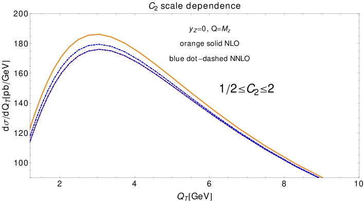
The effect of the inclusion of scale-dependent terms at ${\cal O}(\alpha_{s}^{2})$ is illustrated in Fig. 1 for the $Q_{T}$ differential cross section for Tevatron $Z$ production at the central rapidity $y_{Z}=0$ and $Q=M_{Z}$. The orange solid band is the ${\cal O}(\alpha_{s})$ uncertainty obtained by variations of $C_{2}$ in the range $0.5-2$, while the blue dot-dashed band is the same uncertainty evaluated at ${\cal O}(\alpha_{s}^{2})$. The sensitivity of the cross section to $C_{2}$ is clearly reduced upon the inclusion of the ${\cal O}(\alpha_{s}^{2})$ contribution.

2.5 Nonperturbative resummed contributions

Our fit to the $\phi^{*}_{\eta}$ will adopt a simple flexible convention [32] for $\widetilde{W}_{\alpha}(b,Q)$ at $b\gtrsim 1\mbox{ GeV}^{-1}$ that can emulate a variety of functional forms arising in detailed nonperturbative models [72, 14, 73, 74, 75, 76, 46, 43, 44].

The convention is motivated by the observation that, given the strong suppression of the deeply nonperturbative large-$b$ region in $Z$ boson production, only contributions from the transition region of $b$ of about $1$ GeV^-1 are non-negligible compared to the perturbative contribution from $b<1\mbox{ GeV}^{-1}$. In the transition region, $\widetilde{W}(b,Q)$ can be reasonably approximated by the extrapolated leading-power, or perturbative, part $\widetilde{W}^{pert}(b,Q)$, and the nonperturbative smearing factor $\widetilde{W}^{NP}(b,Q)$:

$$\widetilde{W}_{\alpha,j}(b,Q,y_{Z})=\widetilde{W}_{\alpha,j}^{pert}(b_{*},Q,y_{Z})\widetilde{W}^{NP}(b,Q,y_{Z}).$$ (31)

When $b$ is large, the slow $b$ dependence in $\widetilde{W}_{\alpha,j}^{pert}(b_{*},Q)$ can be neglected, compared to the rapidly changing $\widetilde{W}_{NP}(b,Q)$. The latter contribution captures the effect of the powerlike contributions proportional to $b^{p}$ with $p>0$ that alter the large-$b$ tail of $\widetilde{W}(b,Q)$ in a different way compared to $\widetilde{W}^{pert}(b,Q)$. The powerlike contributions suppress the rate only at $Q_{T}$ below 2-3 GeV, while the leading-power term and its scale dependence affect a broader interval of $Q_{T}$ values (see representative figures in Ref. [50]). The nonperturbative suppression results in a characteristic shift of the peak in the $d\sigma/dQ_{T}$ distribution, which is distinct from the scale dependence.

To avoid divergence due to the Landau pole in $\alpha_{s}(\overline{\mu})$ at $\overline{\mu}\rightarrow 0$, we redefine the scales of order $1/b$ in $\widetilde{W}^{pert}(b,Q)$ according to the $b_{*}$ prescription [9, 10] dependent on two parameters [32]. In the Sudakov exponential, the lower limit $(C_{1}/b)^{2}$ is replaced by $\left(C_{1}/b_{*}(b,b_{max})\right)^{2}$, with

$$b_{*}(b,b_{max})\equiv\frac{b}{\sqrt{1+(b/b_{max})^{2}}},$$ (32)

where $b_{max}$ is set to $1.5\mbox{ GeV}^{-1}$ in [32]. To avoid evaluating the PDFs $f_{a/h}(\xi,\mu_{F})$ at a factorization scale $\mu_{F}$ below the initial PDF scale $\mu_{ini}\approx 1\mbox{ GeV}$, we choose $\mu_{F}=C_{3}/b_{*}(b,C_{3}/\mu_{ini})$; it is larger than $\mu_{ini}$ for any $b$. This prescription is preferred by the global fit to Drell-Yan $Q_{T}$ data, where it both preserves the exact perturbative expansion for $\widetilde{W}^{pert}$ at $b<1$ GeV^-1 and improves the agreement with the data.

In a broad range of $Q$ values in the Drell-Yan process, the behavior of experimentally observed $Q_{T}$ distributions is described by [31, 32]

$$\widetilde{W}^{NP}\left(b,Q\right)=\textrm{exp}\left[-b^{2}\left(a_{1}+a_{2}\ln\left(\frac{Q}{2\ Q_{0}}\right)+a_{3}\ln\left(\frac{x^{(0)}_{1}x^{(0)}_{2}}{0.01}\right)\right)\right]\,,$$ (33)

with $x^{(0)}_{1,2}=\frac{Q}{\sqrt{s}}e^{\pm y}$, free parameters $a_{1},\ a_{2},\ a_{3}$, and a fixed dimensional parameter $Q_{0}=1.6$ GeV. The $b^{2}$ dependence characterizes the leading power-suppressed contribution [72] that can be resolved with the available data. The $\ln(Q)$ dependence is predicted by the Collins-Soper evolution equation [8]. The higher-order power-suppressed contributions proportional to $b^{4}$, etc. cannot be reliably distinguished in the fit from the $b^{2}$ term. Although linear contributions proportional to $b$ may also arise from long-distance dynamics [52], they have been empirically disfavored in a global $Q_{T}$ fit [31].

In the vicinity of $Q$ around $M_{Z}$, Eq. (33) reduces to

$$\widetilde{W}^{NP}\left(b,Q\approx M_{Z}\right)=\textrm{exp}\left[-b^{2}a_{Z}\right]$$ (34)

with

$$a_{Z}=a_{1}+a_{2}\ln\left(\frac{M_{Z}}{2\ Q_{0}}\right)+a_{3}\ln\left(\frac{M_{Z}^{2}}{0.01~{}s}\right).$$ (35)

One of the essential applications of CSS resummation formalism concerns the measurement of $W$ boson mass in hadron-hadron collisions. The current most precise $W$ mass measurements obtained by the DØ and CDF collaborations at the Tevatron [77, 78] quote a total error of about 20 MeV, with the bulk of it (approximately 90%) associated with three theoretical sources: PDF uncertainty (of order 10 MeV according to [79]), EW corrections, and the model of $\widetilde{W}_{NP}(b,Q)$ in production of $W$ bosons. The last source of uncertainty appears because the $W$ mass measurements are sensitive to the shape of the cross section in the low-$Q_{T}$ region.

Once $a_{Z}$ is determined from $Z/\gamma^{*}$ boson production, it is easy to predict $\widetilde{W}^{NP}$ in $W$ boson production at the same $\sqrt{s}$:

$$\widetilde{W}^{NP}\left(b,Q\approx M_{W}\right)=\textrm{exp}\left[-b^{2}a_{W}\right],$$ (36)

where

$$a_{W}=a_{Z}+a_{2}\ln\left(\frac{M_{W}}{M_{Z}}\right)+a_{3}\ln\left(\frac{M_{W}^{2}}{M_{Z}^{2}}\right).$$ (37)

For $b_{max}=1.5$ GeV^-1, one finds $a_{2}=0.17\pm 0.03$ GeV² and $a_{3}=-0.03\pm 0.02$ GeV² [32], where the error estimate includes the scale dependence. The log terms proportional to $a_{2}$ and $a_{3}$ are small in Eq. (37), so that it is safe to assume $a_{W}\approx a_{Z}$ in central-rapidity measurements at the same $\sqrt{s}$.

If $Q$ is substantially different from $M_{Z}$, or if predictions for the LHC are made, the $a_{2}$ and $a_{3}$ contributions cannot be neglected. The nonperturbative coefficient becomes

$$a(Q,\sqrt{s})=a_{Z}(1.96\mbox{ TeV})+a_{2}\ln\left(\frac{Q}{M_{Z}}\right)+a_{3}\ln\left(\frac{Q^{2}}{M_{Z}^{2}}\frac{s}{(1.96\mbox{ TeV})^{2}}\right).$$ (38)

2.6 Matching the $W$ and $Y$ terms

By examining the mapping of $Q_{T}$ distributions on $\phi^{*}_{\eta}$ distributions discussed in Sec. 2.1, we can identify three regions with distinct QCD dynamics: the resummation region $\phi^{*}_{\eta}\lesssim 0.1$ rad, where the $W$ term dominates; the intermediate (matching) region $0.1\lesssim\phi^{*}_{\eta}\lesssim 0.5$ rad; and the perturbative region $\phi^{*}_{\eta}\gtrsim 0.5$ rad, where the $W+Y$ term approaches the fixed-order (FO) contribution. As $\phi^{*}_{\eta}$ increases in the intermediate region, the $W+Y$ term eventually becomes smaller than the FO term at $\phi^{*}_{\eta}\equiv\phi_{switch}(Q,y_{Z})$. The final cross section is taken to be equal to the $W+Y$ term at $\phi^{*}_{\eta}<\phi_{switch}$ and FO term at $\phi^{*}_{\eta}\geq\phi_{switch}$ [30].

The position of the switching point is subject to some variations dependent on the shapes of the $W$ term and its asymptotic expansion at not too small $\phi^{*}_{\eta}\propto Q_{T}/Q$, i.e. away from the $Q_{T}^{2}/Q^{2}\rightarrow 0$ limit where the $W$ term is uniquely defined. These variations have almost no effect on the fit of the nonperturbative function in the resummation region $\phi_{\eta}^{*}$. They originate from the possibility of including additional terms of order $Q_{T}^{2}/Q^{2}$ in the longitudinal momentum fractions $\chi_{1,2}$ in the $W$ term and its asymptotic expansion. These terms vanish at $Q_{T}^{2}/Q^{2}\rightarrow 0$, but they can be numerically important or even desirable in the intermediate region, where they may improve agreement between the $W+Y$ and FO terms.

At intermediate $Q_{T}/Q$, radiation of a $Z$ boson and semi-hard jets requires sufficient center-of-mass energy of incident partons, or large enough partonic momentum fractions $\xi_{1}$ and $\xi_{2}$. For example, the FO hadronic cross section is written as

$$\frac{d\sigma}{dQ^{2}dy_{Z}dQ_{T}^{2}}=\sum_{a,b}\int_{0}^{1}d\xi_{1}\int_{0}^{1}d\xi_{2}\frac{d\hat{\sigma}}{dQ^{2}dy_{Z}dQ_{T}^{2}}f_{a/A}(\xi_{1})f_{b/B}(\xi_{2})$$

$$\equiv\int_{\bar{\xi}_{1}}^{1}d\xi_{1}\int_{\bar{\xi}_{2}}^{1}d\xi_{2}h(\xi_{1},\xi_{2})~{}\delta\left[\left(\frac{\xi_{1}}{x_{1}}-1\right)\left(\frac{\xi_{2}}{x_{2}}-1\right)-\frac{Q_{T}^{2}}{M_{T}^{2}}\right]\,,$$ (39)

where $h(\xi_{1},\xi_{2})$ contains the hard-scattering matrix element and PDFs, and $M_{T}=\sqrt{Q^{2}+Q_{T}^{2}}$. The energy constraint from the $\delta$-function imposes the following boundaries on the partonic momentum fractions: $\xi_{1}=x_{1}+(Q_{T}^{2}/s)/(\xi_{2}-x_{2})$; $\bar{\xi}_{1}=[x_{1}+(Q_{T}^{2}/s)/(1-x_{2})]\leq\xi_{1}\leq 1$; $\bar{\xi}_{2}\equiv[x_{2}+(Q_{T}^{2}/s)/(1-x_{1})]\leq\xi_{2}\leq 1$, with $x_{1,2}=\frac{M_{T}}{\sqrt{s}}e^{\pm y}$.

These boundaries are absent in the $W$ and asymptotic contributions, which depend on convolutions of Wilson coefficient functions and PDFs,

$$\left[C_{j,a}\otimes f_{a/h_{i}}\right](\chi_{i},\mu_{F})=\int_{\chi_{i}}^{1}\frac{d\xi_{i}}{\xi_{i}}C_{j,a}\left(\frac{\chi_{i}}{\xi_{i}},\mu_{F}b,C_{1},C_{2},C_{3}\right)f_{a/h_{i}}(\xi_{i},\mu_{F})\,$$ (40)

for $i=1$ or $2$. The variables $\chi_{i}$ satisfy $\chi_{1,2}\rightarrow x_{1,2}^{(0)}\equiv(Q/\sqrt{s})e^{\pm y}$ and cannot exceed $\bar{\xi}_{1,2}$. Thus, for non-negligible $Q_{T}^{2}/Q^{2}$, the $W$ and asymptotic term may include contributions from the unphysical momentum fractions $\xi_{i}\leq\bar{\xi}_{i}$, and ideally one should include kinematically important $Q_{T}^{2}/Q^{2}$ contributions into $\chi_{1,2}$ to bring them as close to $\bar{\xi}_{1,2}$ as possible.

As the procedure for including the $Q_{T}^{2}/Q^{2}$ corrections in the $W$ term is not unique, we explored several of them. We find that either $\chi_{1,2}=x^{(0)}_{1,2}=(Q/\sqrt{s})e^{\pm y}$ or $\chi_{1,2}=x_{1,2}=(M_{T}/\sqrt{s})e^{\pm y}$ results in the comparable agreement with the $\phi^{*}_{\eta}$ data from DØ and ATLAS 7 TeV. These prescriptions are designated as the “kinematical corrections of type 0” and “type 1”, or $kc_{0}$ and $kc_{1}$, in our numerical outputs.

In contrast, some alternative choices produce worse agreement with the examined data, such as $\chi_{1,2}=\bar{\xi}_{1,2}=((M_{T}+Q_{T})/\sqrt{s})e^{\pm y}$ designated as $kc_{2}$. Furthermore, the $kc_{1}$ prescription improves matching compared to $kc_{0}$ at $\sqrt{s}=14$ TeV, corresponding to scattering at smaller $x$. We use the $kc_{1}$ matching as the default prescription in the subsequent comparisons.

Dependence on the matching prescription at intermediate $Q_{T}$ (intermediate $\phi_{\eta}^{*}$) reflects residual sensitivity to higher-order contributions and is reduced [30] once large-$Q_{T}$ contributions of ${\cal O}(\alpha_{s}^{2})$ are included, compared to ${\cal O}(\alpha_{s})$. The ResBos implementation follows a general argument for matching of the resummed contribution onto the fixed-order result that applies in other areas, such as the treatment of PDFs for heavy quarks in DIS in a general-mass variable number scheme [80, 81]. Matching is stabilized by constructing resummed coefficient functions that comply with the energy-momentum conservation in the exact fixed-order contribution.

2.7 Photon radiative contributions

Our resummed calculations include both $Z$-mediated and photon-mediated contributions to production of Drell-Yan pairs, as well as their interference. Electroweak radiative contributions have been extensively studied in $Z$ boson [83, 84, 85, 86] and $W$ boson production [87, 88, 89, 90, 91, 92]. The dominant NLO electroweak contribution is associated with final-state radiation of photons. To compare the DØ  data to the ResBos prediction without the NLO electroweak correction, we correct the fitted data to the Born level for final-state leptons by subtracting the NLO EM correction obtained bin-by-bin by the Photos code [93]. This correction is essential for the agreement of ResBos theory and data. However, since the photon-mediated and final-state photon radiation contributions are relatively small, in the first approximation we can treat them as a linear perturbation and evaluate for a fixed combination of the nonperturbative and scale parameters taken either from the BLNY or our best-fit parametrizations.

2.8 Numerical accuracy

Given the complexity of the resummation calculation, we expect several sources of random numerical errors that may compete with the accuracy of the most precise $\phi^{*}_{\eta}$ data points, which are of order 0.5% of the respective central cross sections. The numerical errors may arise from the parametrizations of PDFs, integration, and interpolation at various stages of the analysis. They can be treated as independent and uncorrelated and primarily result in higher-than-normal values of the figure-of-merit function $\chi^{2}$ when not explicitly included in the estimates. In comparison, the variations due to $a_{Z}$ or $C_{1,2,3}$ parameters are of order a few percent and correlated across the $\phi_{\eta}^{*}$ spectrum.

2.9 A comparison with an alternative formalism

In the last part of this section, it is instructive to summarize the distinctions between the NNLL/NNLO resummed $Q_{T}$ distributions obtained in the CSS formalism and the alternative approach of Refs. [82, 19, 28]. Both methods predict $Q_{T}$ distributions in a wide range of processes, including production of lepton pairs and Higgs boson. While sharing the same physics principles, they organize the small-$Q_{T}$ form factor $W$ in distinct ways and differ in the form of their higher-order corrections and quantitative dependence on QCD scales.

We will outline the key differences by referring to the work by Bozzi, Catani, de Florian, and Grazzini (BCFG) in Ref. [82]. There, the BCFG representation was derived step-by-step and compared to the CSS method in the kin process of $gg\rightarrow\mbox{Higgs}$ production. The general observations of that paper also apply to the Drell-Yan process.

In both formalisms, the resummed $Q_{T}$ distribution for $h_{1}h_{2}\rightarrow VX$, where $V=\gamma^{*},Z$, and upon integration over the decay angles of the lepton pair, is constructed from the small-$Q_{T}$ resummed, large-$Q_{T}$ fixed-order, and asymptotic (overlap) contributions, denoted as $W$, FO, and $(W)_{\mbox{FO}}$:

$$\frac{d\sigma\left(h_{1}h_{2}\rightarrow VX\right)}{dQ^{2}\ dy_{Z}\ dQ_{T}^{2}}=W+\mbox{FO}-\left(W\right)_{\mbox{FO}}=W+Y.$$ (41)

In accord with the preceding discussion, the $W$ term of the CSS formalism takes form, in a simplified notation, of

$$W(Q,Q_{T},y_{Z})=\int\frac{bdb}{4\pi}\,J_{0}(Q_{T}b)\widetilde{W}_{CSS}(b,Q,y_{Z}).$$ (42)

The integrand consists of the zeroth order Bessel function, $J_{0}(Q_{T}b)$, and the form factor $\widetilde{W}_{CSS}$ that is derived in the context of TMD factorization. At $b\ll 1\mbox{ GeV}^{-1}$, the form factor is expressed as

$$\widetilde{W}_{CSS}(b,Q,y_{Z})=\sum_{j,a,b}\int_{0}^{1}d\xi_{1}\int_{0}^{1}d\xi_{2}\ f_{a/h_{1}}(\xi_{1},\mu_{F})\,f_{b/h_{2}}(\xi_{2},\mu_{F})$$ (43)

$$\times \left|H_{j}(Q,\mu_{Q}/Q;\alpha_{S}(\mu_{Q}))\right|^{2}\,\exp\left[-\int_{\mu_{b}}^{\mu_{Q}}\frac{d\mu^{2}}{\mu^{2}}A(\alpha_{S}(\mu),\,\mu_{b}b)\,\ln\left(\frac{\mu_{Q}^{2}}{\mu^{2}}\right)+B(\alpha_{S}(\mu),\,\mu_{b}b,\,\mu_{Q}/Q)\right]$$

$$\times {\cal C}_{ja}\left(\frac{\chi_{1}}{\xi_{1}},\frac{\mu_{Q}}{\mu_{b}},\mu_{F}b\right){\cal C}_{\bar{j}b}\left(\frac{\chi_{2}}{\xi_{2}},\frac{\mu_{Q}}{\mu_{b}},\mu_{F}b\right).$$

$\widetilde{W}_{CSS}$ depends on three QCD scales: $\mu_{b}=C_{1}/b$, $\mu_{Q}=C_{2}Q$, $\mu_{F}=C_{3}/b$, where the arbitrary scale constants $C_{1},$ $C_{2}$, and $C_{3}$ are of order unity. Their exact values are chosen so as to optimize the convergence of the perturbative series. The combination $C_{1}=C_{3}=b_{0}$, $C_{2}=1$ is the natural choice.

In Ref. [82, 19], the resummed form factor $\widetilde{W}_{BCFG}$ in the second approach is written at $b\ll 1\mbox{ GeV}^{-1}$ as

$$\widetilde{W}_{BCFG}(b,Q,y_{Z})=$$

$$\sum_{j,a,b}\int_{0}^{1}d\xi_{1}\int_{0}^{1}d\xi_{2}\, f_{a/h_{1}}(\xi_{1},\overline{\mu}_{F})\,f_{b/h_{2}}\xi_{2},\overline{\mu}_{F})\,W_{j,ab}(b,Q,\xi_{1}\xi_{2}s;\overline{\alpha}_{s},\overline{\mu}_{R},\overline{\mu}_{F}).$$ (44)

$W_{j,ab}$ is reconstructed from its $N$-th Mellin moments $W_{ab,N}$ that are expanded in powers of $\alpha_{s}(\overline{\mu}_{R})\equiv\overline{\alpha}_{s}$. $W_{ab,N}$ consists of the function ${\cal H}_{j,ab,N}$ that depends only on scales of order $Q$, and the exponent $e^{{\cal G_{N}}}$ that depends on $\widetilde{L}\equiv\ln(Q^{2}b^{2}/b_{0}^{2}+1)$ and ratios of various scales:

$$W_{ab,N}\left(b,Q;\overline{\alpha}_{s},\overline{\mu}_{R},\overline{\mu}_{F}\right)=$$

$$\quad\quad{\cal H}_{j,ab,N}\left(Q,\overline{\alpha}_{s},Q/\overline{\mu}_{R},Q/\overline{\mu}_{F},Q/\overline{\mu}_{Q}\right)\cdot\exp\left\{{\cal G}_{N}\left(\overline{\alpha}_{s},\widetilde{L};Q/\overline{\mu}_{R},Q/\overline{\mu}_{Q}\right)\right\}.$$ (45)

On the right-hand side, the representation includes three auxiliary QCD scales, each taken to be of order of the boson’s virtuality $Q$: the resummation scale $\overline{\mu}_{Q}$, the renormalization scale $\overline{\mu}_{R}$, and the PDF factorization scale $\overline{\mu}_{F}$. The dependence on $b$ enters only through the logarithmic term $\widetilde{L}$ inside $e^{{\cal G_{N}}}$.

The representation $\widetilde{W}_{BCFG}(b,Q,y_{Z})$ in Eqs. (44, 45) can be obtained from $\widetilde{W}_{CSS}(b,Q,y_{Z})$ in Eq. (43) by a series of steps that are documented in [82].

First, the QCD scales are selected differently in the two approaches. In $\widetilde{W}_{CSS}(b,Q,y_{Z})$ several terms depend on the variable scales $\mu_{b}=C_{1}/b$ and $\mu_{F}=C_{3}/b$. The QCD scale $C_{2}Q$ plays the role that is similar to the resummation scale $\overline{\mu}_{Q}$. Inside the Sudakov integral, the scale $\mu$ in $\alpha_{s}(\mu)$ is integrated over.

In $\widetilde{W}_{BCFG}(b,Q,y_{Z})$, the scales $\overline{\mu}_{b}$ and $\overline{\mu}_{F}$ are fixed at $b_{0}/b$. The QCD coupling strength $\alpha_{s}(\mu)$ is converted into the series of $\overline{\alpha}_{s}$ (at the scale $\overline{\mu}_{R}\sim Q$) using the renormalization group equations. The collinear PDFs $f_{a/h}(\xi,\mu)$ in Eqs. (43) and (44) are evaluated at $\mu_{F}\sim 1/b$ in $\widetilde{W}_{CSS}(b,Q,y_{Z})$, and $\overline{\mu}_{F}\sim Q$ in $\widetilde{W}_{BCFG}(b,Q,y_{Z})$. To preserve the factorization scale invariance, the Mellin moment $W_{ab,N}$ of the BCFG form factor explicitly includes an operator matrix ${\mathbb{U}}_{N}(b_{0}/b,\overline{\mu}_{F})$ for DGLAP evolution of $f_{a/h}(\xi,\mu)$ between the scales $\overline{\mu}_{F}$ and $b_{0}/b$, while the CSS form factor does not.

After the conversion $\alpha_{s}(\mu)\rightarrow\overline{\alpha}_{s}$ in $W_{ab,N}$, the contributions at scales of order $Q$ are included into ${\cal H}_{j,ab,N}$ as in Eq. (45). The Sudakov integral $S(b,Q;C_{1},C_{2})=S(\mu_{Q}/\mu_{b})$ and the anomalous dimensions of various components are assimilated into ${\cal G}_{N}$. Within ${\cal G}_{N}$, all evolution operators are expanded as a series in $\overline{\alpha}_{s}$ and $L=\ln(Q^{2}b^{2}/b_{0}^{2})$:

$${\cal G}_{N}=Lg^{(1)}(\overline{\alpha}_{s}L)+g^{(2)}\left(\overline{\alpha}_{s}L;\frac{Q}{\overline{\mu}_{R}},\frac{Q}{\overline{\mu}_{Q}}\right)+\frac{\overline{\alpha}_{s}}{\pi}\,g^{(3)}\left(\overline{\alpha}_{s}L;\frac{Q}{\overline{\mu}_{R}},\frac{Q}{\overline{\mu}_{Q}}\right)+...$$ (46)

Finally, a prescription for matching of the $W+Y$ and FO terms at large $Q_{T}$ is introduced in $\widetilde{W}_{BCFG}$ by replacing all generic logarithms $L=\ln(Q^{2}b^{2}/b_{0}^{2})$ in $e^{{\cal G}_{N}}$ by $\widetilde{L}=\ln(Q^{2}b^{2}/b_{0}^{2}+1)$. The replacement forces the exponential to satisfy $e^{{\cal G_{N}}}\rightarrow 1$ when $b_{0}^{2}/b^{2}\ll Q^{2}$, i.e., in the region of the small transverse positions $b$ that dominate the Fourier-Bessel integral when $Q_{T}$ is large. The resulting outcome is that the $W$ and asymptotic terms cancel well at large $Q_{T},$ and that, upon the integration over $Q_{T}$, the inclusive $W+Y$ cross section turns out to be exactly equal to the fixed-order cross section. In the BCFG cross section, matching therefore arises as a result of a mathematical replacement $L\rightarrow\widetilde{L}$ in the resummed exponential, and not because of the physical constraint due to energy-momentum conservation imposed in our approach. The $L\rightarrow\widetilde{L}$ matching works by suppressing the ${\cal G_{N}}$ exponent at $b^{2}\ll 1/Q^{2}$ via a deft, even though not unique, redefinition of $L$ (see also Ref. [94]).

In the CSS approach adopted in ResBos, the scale constants $C_{1}$ and $C_{3}$ need not to equal $b_{0}$ exactly. The Sudakov integral $S(\mu_{Q}/\mu_{b})$ is evaluated numerically and not as a logarithmic expansion in powers of $L$ as it is done in $\widetilde{W}_{BCFG}(b,Q,y_{Z})$. The ResBos code does not operate with the independent QCD scales $\overline{\mu}_{R}\sim Q$ and $\overline{\mu}_{F}\sim Q$ of the BCFG formalism.

ResBos finds $\alpha_{s}(\mu)$ by numerically solving the renormalization group equation and always evolves the PDFs $f_{a/h}(\xi,\mu_{F})$ forward from the initial scale $Q_{0}\approx 1$ GeV of the input PDF ensemble to a higher scale $\mu_{F}\geq Q_{0}.$ This is to be contrasted with $\widetilde{W}_{BCFG}(b,Q,y_{Z})$, which implements the logarithmic expansion for $\alpha_{s}(\mu)$ and the DGLAP matrix operator ${\mathbb{U}}_{N}(b_{0}/b,\overline{\mu}_{Q})$ that evolves the PDFs $f_{a/h}(\xi,\overline{\mu}_{F})$ backward from $\overline{\mu}_{Q}\approx Q$ down to a lower scale $b_{0}/b$ in the most relevant $b$ region. The backward evolution of this kind has a tendency to be unstable and cause the PDFs to deviate at low momentum scales. Hence the numerical evolution of $\alpha_{s}(\mu)$ and forward DGLAP evolution adopted in $\widetilde{W}_{CSS}(b,Q,y_{Z})$ is more trustworthy in precision studies.

The nonperturbative contribution arises in $\widetilde{W}_{CSS}(b,Q,y_{Z})$ as a natural feature of QCD factorization in terms of TMD PDFs. Dependence on matching is present, implicitly or explicitly, in either formalism. When looking for evidence of nonperturbative effects in $\phi_{\eta}^{*}$ distributions, it is desirable to investigate several prescriptions for matching of low-$Q_{T}$ and high-$Q_{T}$ terms. We have done it by varying the form of the rescaling variables that control the cross sections in the matching region in ResBos.

3 Numerical results

3.1 General features

In this section we determine $a_{Z}$ from the distribution $(1/\sigma)~{}d\sigma/d\phi^{*}_{\eta}$ measured by DØ  [25] that is normalized to the total cross section $\sigma$ in the measured $Q$ and $y$ range. These data are given in three bins of $Z$ boson rapidity $y_{Z}$. In the first two, $|y_{Z}|\leq 1$ and $1\leq|y_{Z}|\leq 2$, the $(1/\sigma)~{}d\sigma/d\phi^{*}_{\eta}$ distribution is measured separately for electrons and muons at $N_{pt}=29$ points of $\phi^{*}_{\eta}$. In the third bin, $|y_{Z}|\geq 2$, only electrons are measured at 25 points of $\phi^{*}_{\eta}$. The first two $y_{Z}$ bins provide substantial new constraints. The third bin has larger statistical errors and reduced discriminating power.

All predictions are obtained by using CT10 NNLO PDFs [54]. Predictions based on MSTW’08 NNLO PDF sets [95] were also computed and did not show significant difference with CT10 NNLO predictions.

Figure 2: The ratios to the central theoretical prediction of the DØ electron data at $|y_{Z}|\leq 1$ and alternative theoretical predictions. The central prediction is computed assuming $C_{1}=C_{3}=2b_{0}$, $C_{2}=1/2$, $a_{Z}=1.1\mbox{ GeV}^{2}$, and kinematical correction 1. Theory predictions based on alternative kinematical corrections (0 and 2) and BLNY nonperturbative parametrization are also shown.

Figure 3: Electrons: scale variation due to $C_{1,2,3}$ at small $\phi^{*}_{\eta}$.

Figure 4: Same as above but for the muons.

From the previous section, the resummed cross sections depend on the perturbative scales, power-suppressed contributions, and choice of subleading kinematic terms. It is possible to identify an optimal combination of these factors that results in a good description of the DØ data across the full $\phi^{*}_{\eta}$ range. In particular, the large-$Q_{T}$/large-$\phi_{\eta}^{*}$ data generally prefer the factorization scale of order $Q/2$ or even less in the fixed-order piece. At small-$Q_{T}$(small-$\phi_{\eta}^{*}$), the scale parameter $C_{3}$ in the range $1.5b_{0}-2b_{0}$ is slightly more preferable. To illustrate properties of the $\phi_{\eta}^{*}$ distributions, we compute the resummed cross sections using a combination $C_{1}=C_{3}=2\ b_{0}$, $C_{2}=Q/2$, and $a_{Z}=1.1\mbox{ GeV}^{2}$ that is close to the best-fit solution. The difference between the best-fit solution and the prediction based on these round-off values will be discussed in Sec. 3.2.

A comparison of the prediction with these choices to the DØ data for $|y_{Z}|\leq 1$ and a few other predictions is presented in Fig. 2. The new parametrization provides better description of the data at $0.1\leq\phi^{*}_{\eta}\leq 1$ than the superimposed prediction utilizing the BLNY parametrization [31] of $\widetilde{W}^{NP}$. Consequently, it results in a better $\chi^{2}$ than the ResBos prediction used in the DØ analysis [25], which used the CTEQ6.6 NLO PDFs, BLNY $\widetilde{W}_{NP}$, and canonical choice of $C_{1,2,3}$.

We also compare predictions for three types (0, 1, 2) of the kinematical (matching) correction discussed in Sec. 2.6. For the selected combination of scale parameters, the type-0 and 1 kinematical corrections provide a nearly identical prediction. The type-0 and type-1 corrections can differ by 2-3% for other scales. Type 2 is generally disfavored, so that we assume the type-1 correction for the rest of the analysis.

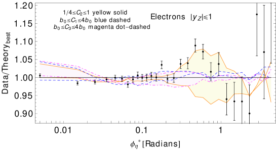
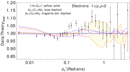
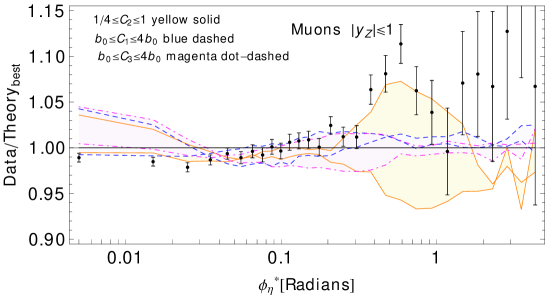
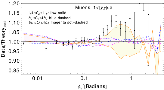
A prediction with the same theoretical parameters, as well as for variations in QCD scales in the ranges $1/4\leq C_{2}\leq 1$ and $b_{0}\leq C_{1,3}\leq 4b_{0}$, are compared to the data for electron production in Fig. 3 and muon production in Fig. 4. Here we show all rapidity bins both for electron and muon samples. The ratios of the DØ data to ResBos theory with the optimal parameters are indicated by black circles. Yellow solid, blue dashed, and magenta dot-dashed bands represent variations in theory due to $C_{2}$, $C_{1}$, and $C_{3}$, respectively, all normalized to the best-fit prediction. Again, the agreement with ResBos observed in these figures is better than in [25]. Figs. 3 and 4 demonstrate that the theoretical uncertainty at small $\phi^{*}_{\eta}$ is dominated by variations of $C_{1}$ and $C_{3}$. The bands of scale uncertainty are reduced significantly for $0.04\leq\phi^{*}_{\eta}\leq 0.1$ upon the inclusion of ${\cal O}(\alpha_{s}^{2})$ scale dependence, as has been discussed in Sec. 2.4.

Figure 5: Dependence on the nonperturbative parameter $a_{Z}$ for electrons with $|y_{Z}|\leq 1$.

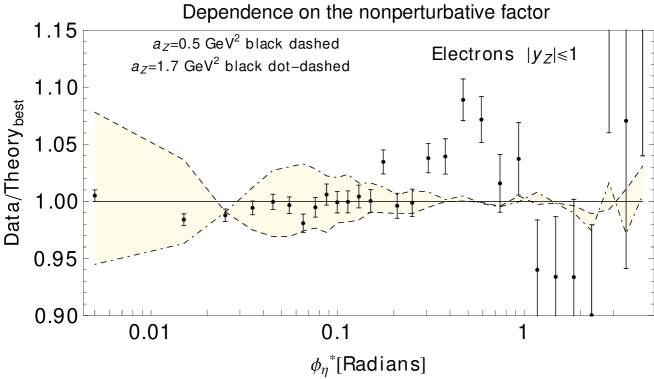
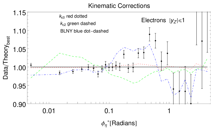
The scale variations can be compared to the dependence on $a_{Z}$ and kinematic correction in Fig. 5, which result in distinctly different patterns of varation in $d\sigma/d\phi^{*}_{\eta}$. In particular, while the perturbative scale coefficients $C_{1},C_{2},C_{3}$ produce a slowly changing variation across most of the measured $\phi^{*}_{\eta}$ range, the increase in $a_{Z}$ produces a distinct variation that suppresses the rate at $\phi^{*}_{\eta}\lesssim 0.02$ and increases it at $0.02\lesssim\phi^{*}_{\eta}\lesssim 0.5$, with the rate above $0.5$ essentially unaffected. A similar behavior was observed in Fig. 6 of [50] with a different NP function and a different procedure that varied all QCD scales around the central values of order of the dilepton’s mass.

It is therefore possible to separate the scale dependence from the $a_{Z}$ dependence if we restrict the attention to $\phi^{*}_{\eta}$ below and around $\phi^{*}_{\eta}=0.1$. To this aim we consider only the first 12 bins of $\phi^{*}_{\eta}$, starting from the smallest value, for each value of rapidity. Extending the fitted range above $\phi^{*}_{\eta}\geq 0.1$ has a minimal effect on $a_{Z}$.

3.2 Detailed analysis

We pursue two approaches for the examination of the low-$\phi^{*}_{\eta}$ region. In method I, we study the dependence on $a_{Z}$ by assuming fixed resummation scales corresponding to half-integer scale parameters, such as $C_{1}/b_{0}=C_{3}/b_{0}=1,C_{2}=1/2$ or $C_{1}/b_{0}=C_{3}/b_{0}=2,C_{2}=1/2$. In this method, the goodness-of-fit function $\chi^{2}$ is minimized with respect to $a_{Z}$ for select combinations of fixed scale parameters. We find that a $\chi^{2}$ minimum with respect to $a_{Z}$ exists in these cases, but, given the outstanding precision of the $\phi^{*}_{\eta}$ data, the best-fit $\chi^{2}/N_{pt}$ remains relatively high, of order 2-3. This is partly due to the numerical noise discussed in Sec.2.8.

The $\chi^{2}$ function can be further reduced by allowing arbitrary $C_{1,2,3}$ parameters, in particular, by taking $C_{2}$ to be below 1/2. In this context, one has to decide on the acceptable range of variations in $C_{1,2,3}$, i.e. the resummation scales.

As computations for multiple combinations of $a_{Z}$ and $C_{1,2,3}$ parameters would be prohibitively CPU-extensive, in method II we first consider a fixed scale combination indicated by $\{\bar{C}_{1},\bar{C}_{2},\bar{C}_{3}\}$ and implement a linearized model for small deviations of the scale parameters from $\bar{C}_{1,2,3}$. The central combination $\bar{C}_{1,2,3}$, namely ${\bar{C}}_{1}={\bar{C}}_{3}=2b_{0}$, ${\bar{C}}_{2}=1/2$, produces good agreement with the data, although not as good as completely free $C_{1,2,3}$. The linearized model is explained in Sec. 3.2.2. It provides a fast estimate of small correlated changes in the $\phi^{*}_{\eta}$ shape of the kind shown in Figs. 3 and 4.

The $\chi^{2}$ function is sampled at discrete $a_{Z}$ values in the interval $a_{Z}=[0.1:3.5]$ GeV² and reconstructed between the sampling nodes by using polynomial interpolation. When the scale variations are allowed, the dependence of $\chi^{2}$ on $a_{Z}$ is asymmetric and very different from a quadratic one.

To account for the asymmetry of the distributions, we quote the central value $\overline{a}_{Z}$ that minimizes $\chi^{2}(a_{Z})$ and the 68% confidence level (C.L.) uncertainty. The probability density function ${\cal P}(a_{Z})$ for $a_{Z}$ in a sample with $N$ points is taken to follow a chi-squared distribution with $N$ degrees of freedom,

$${\cal P}(a_{Z})={\cal P}_{\chi}(N,\chi^{2}(a_{Z}))=\frac{(\chi^{2})^{N/2-1}\exp\left(-\chi^{2}/2\right)}{\Gamma(N/2)\ 2^{N/2}}.$$ (47)

With this, we determine the 68% C.L. intervals $[a_{Z,min},~{}a_{Z,max}]$, where $a_{Z,min}$ and $a_{Z,max}$ are defined implicitly by

$$0.16=\frac{\int^{a_{Z,min}}_{0}{\cal P}(a_{Z})~{}da_{Z}}{\int^{+\infty}_{0}{\cal P}(a_{Z})~{}da_{Z}}\,, 0.84=\frac{\int^{a_{Z,max}}_{0}{\cal P}(a_{Z})~{}da_{Z}}{\int^{+\infty}_{0}{\cal P}(a_{Z})~{}da_{Z}}\,.$$ (48)

For an asymmetric distribution as in method II, the central value $\overline{a}_{Z}$ does not coincide with the middle of the 68% C.L. interval or the mean $a_{Z}$ given by the first moment of the ${\cal P}(a_{Z})$ distribution.

3.2.1 Method I: minimization with fixed scale parameters

Figure 6: $\chi^{2}/N_{pt}$ as a function of $a_{Z}$ with fixed $C_{1,2,3}$.

Fit results for $\phi_{\eta}^{*}\leq 0.1$
	$N_{pt}$	$\chi_{min}^{2}/N_{pt}$	$\overline{a}_{Z}\pm\delta a_{Z}\ (\mbox{GeV}^{2})$
$|y_{Z}|\leq 1$,   $e+\mu$	24	3.24	$0.79_{-0.03}^{+0.2}$
		2.83	$1.14\pm 0.08$
$1\leq|y_{Z}|\leq 2$,   $e+\mu$	24	1.87	$0.79\pm 0.05$
		3.03	$1.12_{-0.13}^{+0.14}$
$|y_{Z}|\geq 2$,   $e$	12	0.74	$0.8_{-0.05}^{+0.03}$
		0.58	$1.04_{-0.16}^{+0.18}$
All $y_{Z}$ bins,	60	2.19	$0.79\pm 0.03$
weighted average		2.46	$1.12\pm 0.07$

Table 1: The best-fit $\chi^{2}/N_{pt}$, central value and 68% C.L. intervals for $a_{Z}$ with fixed $C_{1,2,3}=\{b_{0},\ 1/2,\ b_{0}\}$ (upper lines) and $\{2b_{0},\ 1/2,\ 2b_{0}\}$ (lower lines).

In method I, $a_{Z}$ is determined from the DØ data by minimization of a function

$$\chi^{2}(a_{Z})=\sum_{i=1}^{N_{pt}}\left(\frac{D_{i}-\bar{T}_{i}(a_{Z})}{s_{i}}\right)^{2},$$ (49)

where $D_{i}$ are the data points; $\bar{T}_{i}(a_{Z})$ are the theoretical predictions for fixed scale parameters $\{\bar{C}_{1},\bar{C}_{2},\bar{C}_{3}\}$; $s_{i}$ are the uncorrelated experimental uncertainties; and $N_{pt}$ is the number of points.

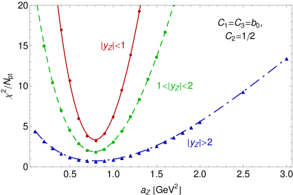
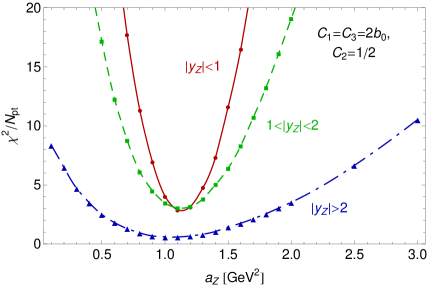
The dependence of $\chi^{2}$ on $a_{Z}$ in three rapidity bins for two combinations of $\bar{C}_{1,2,3}$ is illustrated in Fig. 6, and the corresponding best-fit parameters are listed in Table 1. Electrons and muons are combined in the first two bins of rapidity, $|y_{Z}|\leq 1$ and $1\leq|y_{Z}|\leq 2$. In both cases, the $\chi^{2}$ behavior is close to parabolic. The locations of the $\chi^{2}$ minima are consistent in all three bins. However, the quality of the fit is unacceptable in the first two bins that have the smallest experimental errors, with $\chi^{2}/N_{pt}\approx 3$. On the other hand, the agreement is very good ($\chi^{2}/N_{pt}<1$) in the third bin, which has larger errors.

The weighted averages over all three bins are $\bar{a}_{Z,\mbox{all y}}=0.79\pm 0.03$ and $1.12\pm 0.07$ GeV² for the two scale combinations. The location of the minimum is distinct from zero in both cases, but its dependence on the scale parameters warrants further investigation that we will now perform.

3.2.2 Method II: computation with scale-parameter shifts

To simplify the minimization when the scale parameters are varied, we introduce a linearized approximation for the covariance matrix of the type adopted for evaluating correlated systematic effects in PDF fits [96, 97]. For each scale parameter $C_{\alpha}$, $\alpha=1,2,3$, we define a nuisance parameter $\lambda_{\alpha}\equiv\log_{2}(C_{\alpha}/\bar{C}_{\alpha})$ and compute the finite-difference derivatives of theory cross sections

$$\beta_{i\alpha}\equiv\frac{T_{i}(a_{Z},\lambda_{\alpha}=+1)-T_{i}(a_{Z},\lambda_{\alpha}=-1)}{2}, \alpha=1,2,3;~{}~{}~{}i=1,\dots,N_{pt}\,$$ (50)

over the interval $\lambda_{\alpha}=\pm 1$ corresponding to $\bar{C}_{\alpha}/2\leq C_{\alpha}\leq 2\bar{C}_{\alpha}$. Variations of $\lambda_{\alpha}$ introduce correlated shifts in theory cross sections $T_{i}(a_{Z},C_{1,2,3})$ with respect to the fixed-scale theory cross sections $T_{i}(a_{Z},\bar{C}_{1,2,3})\equiv\bar{T}_{i}(a_{Z})$. We can reasonably assume that the probability distribution over each $\lambda_{\alpha}$ is similar to a Gaussian one with a central value of 0 and half-width $\sigma_{\lambda}$, taken to be the same for all $\lambda_{\alpha}$. The goodness-of-fit function is then defined as

$$\chi^{2}(a_{Z},\lambda_{1,2,3})=\sum_{i=1}^{N_{pt}}\left(\frac{D_{i}-\bar{T}_{i}(a_{Z})-\sum_{\alpha=1}^{3}\beta_{\alpha i}\lambda_{\alpha}}{s_{i}}\right)^{2}+\sum_{\alpha=1}^{3}\frac{\lambda^{2}_{\alpha}}{\sigma_{\lambda}^{2}}.$$ (51)

The minimum with respect to $\lambda_{\alpha}$ can be found algebraically for every $a_{Z}$ as [96]

$$\min\chi^{2}=\chi^{2}(a_{Z},\bar{\lambda}_{\alpha})=\sum_{i,j}^{N_{pt}}(D_{i}-\bar{T}_{i}(a_{Z}))({\rm cov^{-1}})_{ij}(D_{j}-\bar{T}_{j}(a_{Z})),$$ (52)

containing the inverse of the covariance matrix,

$$({\rm cov}^{-1})_{ij}=\left[\frac{\delta_{ij}}{s_{i}^{2}}-\sum_{\alpha,\beta=1}^{3}\frac{\beta_{i,\alpha}}{s_{i}^{2}}\mathcal{A}_{\alpha\beta}^{-1}\frac{\beta_{j,\beta}}{s_{j}^{2}}\right],$$ (53)

and a matrix ${\mathcal{A}}$ given by

$$\mathcal{A_{\alpha\beta}}=\sigma_{\lambda}^{2}\delta_{\alpha\beta}+\sum_{k=1}^{N_{pt}}\frac{{\beta}_{k,\alpha}\beta_{k,\beta}}{s_{k}^{2}}.$$ (54)

Eq. (52) is essentially the standard $\chi^{2}$ function based on the covariance matrix in the presence of the correlated shifts. For every $a_{Z}$, the nuisance parameters $\bar{\lambda}_{\alpha}$ that realize the $\chi^{2}$ minimum are also known,

$$\bar{\lambda}_{\alpha}(a_{Z})=\sum_{i=1}^{N_{pt}}\frac{D_{i}-\bar{T}_{i}(a_{Z})}{s_{i}}\sum_{\delta=1}^{3}\mathcal{A}_{\alpha\delta}^{-1}\frac{\beta_{i,\delta}}{s_{i}}.$$ (55)

Figure 7: $\chi^{2}/N_{pt}$ and scale parameters as a function of $a_{Z}$ for $\bar{C}_{1}=\bar{C}_{3}=2\ b_{0},\bar{C}_{2}=1/2$. The scale parameters are shared across three $y_{Z}$ bins.

Fit results for $\phi_{\eta}^{*}\leq 0.1$
$C_{1},$$C_{2},$ $C_{3}$ are shared by all $y_{Z}$ bins
	$N_{pt}$	$\chi_{min}^{2}/N_{pt}$	$\overline{a}_{Z}\pm\delta a_{Z}\ (\mbox{GeV}^{2})$	Best-fit $C_{1,2,3}$
All $y_{Z}$ bins	60	1.29	$0.82_{-0.12}^{+0.34}$	1.4, 0.33, 1.23
		1.31	$0.82_{-0.11}^{+0.22}$	1.42, 0.33, 1.23
$C_{1},$$C_{2},$ $C_{3}$ are independent in each $y_{Z}$ bin
	$N_{pt}$	$\chi_{min}^{2}/N_{pt}$	$\overline{a}_{Z}\pm\delta a_{Z}\ (\mbox{GeV}^{2})$	Best-fit $C_{1,2,3}$
$|y_{Z}|\leq 1$,   $e+\mu$	24	1.0	$0.56_{-0.02}^{+0.95}$	0.21, 0.18, 7.56
		1.16	$0.85_{-0.15}^{+0.3}$	1.47, 0.3, 1.46
$1\leq|y_{Z}|\leq 2$,   $e+\mu$	24	1.48	$1.22_{-0.36}^{+0.27}$	18, 0.58,0.1
		1.70	$0.79_{-0.1}^{+0.2}$	1.69, 0.37, 0.77
$|y_{Z}|\geq 2$,   $e$	12	-	-	-
		0.59	$0.99_{-0.31}^{+0.99}$	1.74, 0.48, 2.12
Weighted average	60		$0.97\pm 0.25$
of all bins			$0.82\pm 0.12$

Table 2: The best-fit $\chi^{2}/N_{pt}$, central value and 68% C.L. intervals for $a_{Z}$, and best-fit $C_{1,2,3}$ for $1/\sigma_{\lambda}=0$ (upper rows in each section) and $1$ (lower rows).

Based on this representation for $\chi^{2}$ (designated as “fitting method II”), we explored the impact of the scale dependence on the constraint on $a_{Z}$. Even if the scales are varied, data prefer a nonzero nonperturbative Gaussian smearing of about the same magnitude as in method I.

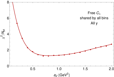
In the simplest possible case, the $C_{1,2,3}$ parameters are independent of the rapidity or other kinematic parameters and shared by all $e$ and $\mu$ bins. In this case, variations of the scale parameters reduce $\chi^{2}/N_{pt}$ to about 1.3, i.e. the fit is better than for the fixed scale combinations discussed above. We focus on the case when the central scale parameters are $\bar{C}_{1}=\bar{C}_{3}=2\ b_{0},C_{2}=1/2$, although the conclusions remain the same for other choices.

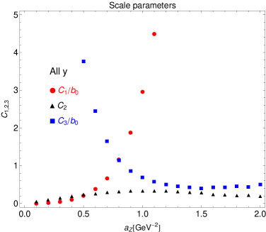
The plots of $\chi^{2}/N_{pt}$ vs. $a_{Z}$ and optimal $C_{1}/b_{0}$, $C_{2}$, $C_{3}/b_{0}$ vs. $a_{Z}$, derived from the optimal $\lambda_{\alpha}$ parameters in Eq. (55), are shown in Fig. 7. The $\chi^{2}$ dependence on $a_{Z}$ becomes asymmetric when the scale shifts are allowed, with the large-$a_{Z}$ branch being flattened out in contrast to the small-$a_{Z}$ one that remains steeply growing. From the right inset, we see that the optimal $C_{1}$ and $C_{3}$ are monotonously increasing and decreasing as functions of $a_{Z}$, respectively. In the vicinity of the minimum, $C_{1}$ and $C_{3}$ are of about the same magnitude at $(1.2-1.5)b_{0}$. Very small or large $a_{Z}$ can be obtained only by taking $C_{1}$ and $C_{3}$ to be uncomfortably far from unity. In contrast, the optimal $C_{2}$ parameter is generally in the range 0.3-0.5 and has weaker dependence on $a_{Z}$.

The values of $\chi^{2}/N_{pt}$, $a_{Z}$, and $C_{1,2,3}$ parameters at the minimum are reported in the upper portion of Table 2. When the $C_{1,2,3}$ parameters are shared by all bins, the fit is relatively insensitive to the confidence level assigned to the variations $\lambda_{\alpha}\pm 1$, controlled by the parameter $\sigma_{\lambda}$ in Eq. (51). In Table 1, the upper rows in each section correspond to the fit without a constraint on the $\lambda$ parameters, i.e., for $1/\sigma_{\lambda}=0$. The lower rows are for assigning a 68% probability to the $-1\leq\lambda_{\alpha}\leq 1$ intervals, corresponding to $1/\sigma_{\lambda}=1$.

For the shared $C_{1,2,3}$, the outcomes of the fits with $1/\sigma_{\lambda}=0$ and 1 are very similar, apart from the uncertainty on the $a_{Z}$ parameter, which is increased when the $\lambda_{\alpha}$ variations are totally free. [The asymmetric 68% C.L. uncertainties are computed according to Eq. (48)].

Figure 8: $\chi^{2}/N_{pt}$ as a function of $a_{Z}$ for $\bar{C}_{1}=\bar{C}_{3}=2\ b_{0},\bar{C}_{2}=1/2$. The scale parameters are independent in each $y_{Z}$ bin.

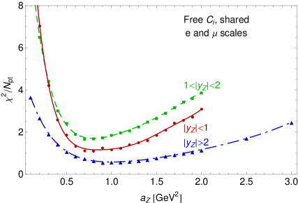
In contrast, when the scale parameters are taken to be independent in each $y_{Z}$ bin (but still shared between the electron and muon samples), only the case of $\sigma_{\lambda}=1$ results in an acceptable fit in all three $y_{Z}$ bins. The best-fit parameters for this case are listed in the lower part of Table 2. When the scale shifts were arbitrary ($1/\sigma_{\lambda}=0$, upper lines), the fits were underconstrained and produced inconsistent $a_{Z}$ values and large scale shifts in all three bins, especially in the third bin that is not shown for this reason. On the other hand, for $\sigma_{\lambda}=1$ (lower lines), the three fits converged well and rendered compatible $a_{Z}$ values. The $\chi^{2}/N_{pt}$ vs. $a_{Z}$ dependence for this case is illustrated in Fig. 8, where the minima are neatly aligned in the three bins. The fit to the second bin is generally worse than for the other two, suggesting possible rapidity dependence of $a_{Z}$. The scale dependence in each bin is qualitatively similar to that in the right inset of Fig. 7.

Figure 9: 68% C.L. ranges for $a_{Z}$ in individual $y_{Z}$ bins and in all bins.

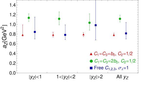
Even when $C_{1,2,3}$ are independent in each $y_{Z}$ bin, by averaging the $a_{Z}$ values over three bins, we obtain the $\bar{a}_{Z}=0.8-0.9\mbox{ GeV}^{2}$ in the last section of Table 2 that is essentially the same as in the case when $C_{1,2,3}$ are shared by all bins. The findings in Tables 1 and 2 are recapitulated in Fig. 9, showing the 68% C.L. intervals in the fits with fixed $C_{1,2,3}={b_{0},1/2,b_{0}}$ and ${2b_{0},1/2,2b_{0}}$, as well as the fit with varied $C_{1,2,3}$ and $\sigma_{\lambda}=1$. All fits consistently yield $a_{Z}$ values that are at least 5$\sigma$ from zero.

4 Implications for the $W$ mass measurement and LHC

The previous sections demonstrated that the $\phi^{*}_{\eta}$ distributions in $Z/\gamma^{*}$ production are sensitive to several QCD effects. Depending on the $\phi^{*}_{\eta}$ range, hard or soft QCD emissions can be studied. The nonperturbative power corrections in QCD can be determined at $\phi^{*}_{\eta}\leq 0.1$, provided that the dependence on resummation scales is controlled.

To distinguish between various contributing effects, new developments in the Collins-Soper-Sterman resummation formalism were necessitated. The computer code ResBos includes all such effects relevant for computation of resummed differential distributions of lepton pairs. New components of the theoretical framework implemented in ResBos were reviewed in Sec. 2. In the large-$\phi_{\eta}^{*}$ region dominated by hard emissions, the two-loop fixed-order contributions implemented in ResBos show good agreement with the DØ data when the renormalization/factorization scale $C_{4}Q$ for hard emissions is set to be close to $Q/2$.

In the resummed $W$ piece dominating at small $\phi^{*}_{\eta}$, we include 2-loop perturbative coefficients in the resummed $W$ term by using the exact formulas for the ${\cal A}$ and ${\cal B}$ coefficients and a numerical estimate for the small ${\cal O}(\alpha_{s}^{2})$ contribution $\delta C^{(2)}$ to the Wilson coefficient functions. We also fully include, up to ${\cal O}(\alpha_{s}^{2})$, the dependence on resummation scale parameters $C_{1}$ and $C_{2}$, (see Secs. 2.3 and 2.4). Matching corrections and final-state electroweak contributions were implemented and investigated in order to understand their non-negligible impact on the cross sections. Finally, we implemented a form factor $\widetilde{W}_{NP}(b,Q)$ describing soft nonperturbative emissions at transverse positions $b\gtrsim 1\mbox{ GeV}^{-1}$ in the context of a two-parameter $b_{*}$ model [32], cf. Sec. 2.5.

With this setup, we performed a study of the small-$\phi^{*}_{\eta}$ region at the DØ Run-2 with the goal to determine the range of plausible nonperturbative contributions. We found that, to describe Drell-Yan dilepton production with the invariant mass $70\leq Q\leq 110$ GeV, it suffices to use a simplified nonperturbative form factor that retains only a leading power correction, $\widetilde{W}_{NP}(b,Q=M_{Z})=\exp\left(-b^{2}a_{Z}\right)$. The power correction modifies the shape of $d\sigma/d\phi^{*}_{\eta}$ in a pattern distinct from variations due to the dependence on the resummation scales $C_{1}/b$, $C_{2}Q$, and $C_{3}/b$ in the leading-power term $\widetilde{W}^{pert}$, see Figs. 3, 4, and 5. For various fixed combinations of scale parameters $C_{1,2,3}$, or when the scale parameters were varied, the fits require nonzero $a_{Z}$ values that were summarized in Tables 1 and 2. For example, when the variations in the scales $C_{1,2,3}$ were incorporated as shared free parameters in all rapidity bins using a correlation matrix, we obtained $a_{Z}=0.82^{+0.22}_{-0.11}\mbox{ GeV}^{2}$ at 68% C.L., cf. Table 2, consistently with the other tried methods. The estimate of the 68% C.L. uncertainty including the scale dependence indicates clear preference for a non-zero $a_{Z}$, without appreciable rapidity dependence.

The magnitude of $a_{Z}$ depends on the resummation scales, but allowing the scales to vary increases the probability for having larger, not smaller $a_{Z}$. The best-fit $a_{Z}$ is also correlated with $b_{max}$, which controls the upper boundary of the $b$ range where the exact perturbative approximation for $\widetilde{W}^{pert}(b,Q,y_{Z})$ is used. Using $b_{max}=1.5\mbox{ GeV}^{-1}$ in this study, we obtain $a(b,Q)\approx 0.8\mbox{ GeV}^{2}$ at $Q=M_{Z}$, which is consistent with the value obtained with the other $\widetilde{W}_{NP}$ forms maximally preserving the perturbative contribution [74, 75, 76, 32]. The dependence on $b_{max}$ weakens at $b_{max}$ above $1\mbox{ GeV}^{-1}$, and even larger $a_{Z}$ values are preferred for $b_{max}$ below $1\mbox{ GeV}^{-1}$, cf. Fig. 2 in [32]. The fitted data was corrected for the effects of final-state NLO QED radiation. In the fitted region $\phi^{*}_{\eta}<0.1$, the uncertainty due to the matching of the resummed and finite-order terms was shown to be negligible.

The nonperturbative form factor at other $\sqrt{s}$ and $Q$ values can be predicted using the relations in Sec. 2.5. This is possible because the dominant part of $\widetilde{W}_{NP}$ is associated with the soft factor $\exp\left(-S(b,Q)\right)$ which does not depend on $\sqrt{s}$ or the types of the incident hadrons. It is argued in Sec. 2.5 that the $\widetilde{W}_{NP}$ factors are identical within the 68% C.L. error in central-rapidity $Z$ and $W$ production at the same $\sqrt{s}$. The same $a_{Z}$ value that we determined can be readily applied to predict $W$ boson differential distributions at the Tevatron Run-2, or, with appropriate modifications proportional to $\ln(Q)$ and $\ln(s)$, in other kinematical ranges, cf. Eq. (38).

The resummation calculation employed in this analysis can be reproduced using the ResBos-P code [98] and input tables  [99] available at the “$Q_{T}$ resummation portal at Michigan State University”. The central input tables are provided for $a_{Z}=1.12\pm 0.07\mbox{ GeV}^{2}$, $C_{1}=C_{3}=2b_{0}$, $C_{2}=1/2$, and central CT10 NNLO PDF. In addition, the distribution includes ResBos tables corresponding to the best-fit resummed parameters and CT10 NNLO PDF eigenvector sets. Finally, for a detailed exploration of the low-$\phi^{*}_{\eta}$ region, the distribution includes tables for $a_{Z}$ in the interval $0.5-1.7\mbox{ GeV}^{2}$ with step $0.1\mbox{ GeV}^{2}$ using the central PDF, and, to study scale dependence, 7 ResBos grids for the central $a_{Z,central}=1.12$ GeV², and the scale parameters $C_{1}={b_{0},4b_{0}}$, $C_{2}={1/4,1}$, and $C_{3}={b_{0},4b_{0}}$.

Figure 10: Data vs. theory ratios for the $Q_{T}$ distribution by ATLAS 7 TeV, $35-40\mbox{ pb}^{-1}$ [26] and $\phi^{*}_{\eta}$ distribution ATLAS 7 TeV, $4.6\mbox{ fb}^{-1}$ [27]

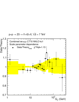
As an example of a phenomenological application, Fig. 10 compares the ResBos predictions with the ATLAS data [26, 27] on Drell-Yan pair production near the $Z$ boson resonance peak at $\sqrt{s}=7$ TeV. The figure shows ratios of data to theory cross sections. The left subfigure shows the $Q_{T}$ distribution for $35-40\mbox{ pb}^{-1}$, compared to the ResBos prediction with $a_{Z}=1.1$ GeV², $C_{1}=C_{3}=2\ b_{0},C_{2}=1/2$. The yellow band indicates variations in the cross section due to the scales in the range $C_{1}={b_{0},4b_{0}}$, $C_{2}={1/4,1}$, and $C_{3}={b_{0},4b_{0}}$. In the case of $Q_{T}$ distribution, we obtain good agreement between theory and data and in the intermediate/small $Q_{T}$ region the theoretical uncertainty due to $C_{1,2,3}$ scale parameters is reduced compared to the study of Ref. [20].

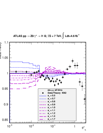
The right subfigure shows the ratio of the more recent $\phi^{*}_{\eta}$ distribution to the central theory prediction based on our default parametrization at much higher level of accuracy. Here, a ResBos prediction based on the BLNY parametrization has shown better agreement with the data than other available codes and was used for event simulation during the ATLAS analysis. A comparable, although somewhat worse agreement is realized by the GNW parametrization, which was not used at any stage by ATLAS. The right subfigure shows several curves for the default $C_{1,2,3}$ choice and $a_{Z}$ in the range $0.5-1.7\mbox{ GeV}^{2}$. It is clear that the ATLAS $\phi^{*}_{\eta}$ data is sensitive to $a_{Z}$ as well as $b_{max}$ and can possibly discriminate subleading power contributions to the nonperturbative form factor $\widetilde{W}_{NP}(b,Q)$ proportional to $b^{4}$ and beyond. We provide sets of updated ResBos grids for the LHC kinematics that can be used for future improvements in the nonperturbative model.

5 Conclusions

In our analysis we have shown that a significant nonperturbative Gaussian smearing is necessary to describe features of the low $\phi^{*}_{\eta}$ spectrum. A non-zero NP function is present even if all the perturbative scale parameters of the CSS formalism are varied. Values of $a_{Z}$ smaller than $0.5$ GeV² are disfavoured by the fit to the recent DØ data, as demonstrated in Sec. 3. The dependence of the $d\sigma/d\phi_{\eta}^{*}$ on various factors was recently examined in [50], and it was observed that the dependence of on the nonperturbative contributions could not be reliably separated from the dependence on the perturbative QCD scales. To go beyond the analysis of Ref. [50], we carried out a quantitative fit to the $\phi_{\eta}^{*}$ data of DØ , in which we implemented the dependence on the soft resummation scales to NNLO, cf. Sec. 2.4. We found that the small-$\phi^{*}_{\eta}$ spectrum cannot be fully described by employing perturbative scale variations only. From the characteristic suppression of the production rate at very small $\phi_{\eta}^{*}$, or very small $Q_{T}/Q$, we established the magnitude of the nonperturbative effects.

The resummed predictions based on the new nonperturbative form are implemented in the ResBos code. It will be of particular interest to explore the constraining power of the new forthcoming LHC data for $Z$ and $W$ production at a variety of $\sqrt{s}$, boson’s invariant masses, and rapidities. Precise measurements of hadronic cross sections at small $Q_{T}$ will verify the TMD formalism for QCD factorization and shed light on the nonperturbative QCD dynamics. These developments will depend on consistent combination of NNLO QCD and NLO electroweak effects and reduction of perturbative scale dependence in QCD predictions for $Q_{T}$ distributions.

References

- [1] P.B. Arnold and M.H. Reno, Nucl.Phys. B319 (1989) 37.
- [2] C. Anastasiou, L. Dixon, K. Melnikov and F. Petriello, Phys.Rev. D69 (2004) 094008, hep-ph/0312266.
- [3] S. Catani, L. Cieri, G. Ferrera, D. de Florian and M. Grazzini, Phys.Rev.Lett. 103 (2009) 082001, 0903.2120.
- [4] G. Bozzi, S. Catani, G. Ferrera, D. de Florian and M. Grazzini, Phys.Lett. B696 (2011) 207, 1007.2351.
- [5] Y.L. Dokshitzer, D. Diakonov and S. Troian, Phys.Lett. B79 (1978) 269.
- [6] G. Parisi and R. Petronzio, Nucl.Phys. B154 (1979) 427.
- [7] G. Curci, M. Greco and Y. Srivastava, Nucl.Phys. B159 (1979) 451.
- [8] J.C. Collins and D.E. Soper, Nucl.Phys. B193 (1981) 381.
- [9] J.C. Collins and D.E. Soper, Nucl.Phys. B197 (1982) 446.
- [10] J.C. Collins, D.E. Soper and G.F. Sterman, Nucl.Phys. B250 (1985) 199.
- [11] J.C. Collins and A. Metz, Phys.Rev.Lett. 93 (2004) 252001, hep-ph/0408249.
- [12] J.C. Collins, Foundations of perturbative QCD (Cambridge University Press, 2011).
- [13] C. Balazs, J. Qiu and C.-P. Yuan, Phys.Lett. B355 (1995) 548, hep-ph/9505203.
- [14] R.K. Ellis and S. Veseli, Nucl.Phys. B511 (1998) 649, hep-ph/9706526.
- [15] D. de Florian and M. Grazzini, Phys.Rev.Lett. 85 (2000) 4678, hep-ph/0008152.
- [16] S. Catani, D. de Florian and M. Grazzini, Nucl.Phys. B596 (2001) 299, hep-ph/0008184.
- [17] D. de Florian and M. Grazzini, Nucl.Phys. B616 (2001) 247, hep-ph/0108273.
- [18] S. Catani and M. Grazzini, Phys.Rev.Lett. 98 (2007) 222002, hep-ph/0703012.
- [19] G. Bozzi, S. Catani, G. Ferrera, D. de Florian and M. Grazzini, Nucl.Phys. B815 (2009) 174, 0812.2862.
- [20] A. Banfi, M. Dasgupta, S. Marzani and L. Tomlinson, Phys.Lett. B715 (2012) 152, 1205.4760.
- [21] A. Banfi, M. Dasgupta and S. Marzani, Phys.Lett. B701 (2011) 75, 1102.3594.
- [22] A. Banfi, M. Dasgupta and R.M. Duran Delgado, JHEP 0912 (2009) 022, 0909.5327.
- [23] P.M. Nadolsky, AIP Conf.Proc. 753 (2005) 158, hep-ph/0412146.
- [24] A. Banfi, S. Redford, M. Vesterinen, P. Waller and T.R. Wyatt, Eur.Phys.J. C71 (2011) 1600, 1009.1580.
- [25] DØ Collaboration, V.M. Abazov et al., Phys.Rev.Lett. 106 (2011) 122001, 1010.0262.
- [26] ATLAS Collaboration, G. Aad et al., Phys.Lett. B705 (2011) 415, 1107.2381.
- [27] ATLAS Collaboration, G. Aad et al., Phys.Lett. B720 (2013) 32, 1211.6899.
- [28] S. Catani, L. Cieri, D. de Florian, G. Ferrera and M. Grazzini, Eur.Phys.J. C72 (2012) 2195, 1209.0158.
- [29] G. Ladinsky and C.-P. Yuan, Phys.Rev. D50 (1994) 4239, hep-ph/9311341.
- [30] C. Balazs and C.-P. Yuan, Phys.Rev. D56 (1997) 5558, hep-ph/9704258.
- [31] F. Landry, R. Brock, P.M. Nadolsky and C.-P. Yuan, Phys.Rev. D67 (2003) 073016, hep-ph/0212159.
- [32] A.V. Konychev and P.M. Nadolsky, Phys.Lett. B633 (2006) 710, hep-ph/0506225.
- [33] J.C. Collins and F. Hautmann, Phys.Lett. B472 (2000) 129, hep-ph/9908467.
- [34] J.C. Collins and F. Hautmann, JHEP 0103 (2001) 016, hep-ph/0009286.
- [35] A. Henneman, D. Boer and P. Mulders, Nucl.Phys. B620 (2002) 331, hep-ph/0104271.
- [36] A.V. Belitsky, X. Ji and F. Yuan, Nucl.Phys. B656 (2003) 165, hep-ph/0208038.
- [37] D. Boer, P. Mulders and F. Pijlman, Nucl.Phys. B667 (2003) 201, hep-ph/0303034.
- [38] J.C. Collins, Acta Phys.Polon. B34 (2003) 3103, hep-ph/0304122.
- [39] J. Collins, T. Rogers and A. Stasto, Phys.Rev. D77 (2008) 085009, 0708.2833.
- [40] A. Idilbi, X.d. Ji and F. Yuan, Phys.Lett. B625 (2005) 253, hep-ph/0507196.
- [41] I. Cherednikov and N. Stefanis, Phys.Rev. D77 (2008) 094001, 0710.1955.
- [42] I. Cherednikov and N. Stefanis, Phys.Rev. D80 (2009) 054008, 0904.2727.
- [43] M.G. Echevarriá, A. Idilbi and I. Scimemi, JHEP 1207 (2012) 002, 1111.4996.
- [44] M.G. Echevarriá, A. Idilbi, A. Schäfer and Ignazio Scimemi, Eur.Phys.J. C73 (2013) 2636, 1208.1281.
- [45] S.M. Aybat and T.C. Rogers, Phys.Rev. D83 (2011) 114042, 1101.5057.
- [46] T. Becher, M. Neubert and D. Wilhelm, JHEP 1202 (2012) 124, 1109.6027.
- [47] S. Mantry and F. Petriello, Phys.Rev. D83 (2011) 053007, 1007.3773.
- [48] S. Mantry and F. Petriello, Phys.Rev. D84 (2011) 014030, 1011.0757.
- [49] S. Berge, P. Nadolsky, F. Olness and C.-P. Yuan, Phys.Rev. D72 (2005) 033015, hep-ph/0410375.
- [50] A. Banfi, M. Dasgupta, S. Marzani and L. Tomlinson, JHEP 1201 (2012) 044, 1110.4009.
- [51] J. Collins, Int.J.Mod.Phys.Conf.Ser. 25 (2014) 1460001, 1307.2920.
- [52] P. Schweitzer, M. Strikman and C. Weiss, JHEP 1301 (2013) 163, 1210.1267.
- [53] M. Guzzi and P.M. Nadolsky, Int.J.Mod.Phys.Conf.Ser. 20 (2012) 274, 1209.1252.
- [54] J. Gao, M. Guzzi, J. Huston, H.-L. Lai, Z. Li, P. Nadolsky, J. Pumplin, D. Stump, C.-P. Yuan, Phys.Rev. D89 (2014) 033009, 1302.6246.
- [55] J.C. Collins and D.E. Soper, Phys.Rev. D16 (1977) 2219.
- [56] A. Banfi, M. Dasgupta and Y. Delenda, Phys.Lett. B665 (2008) 86, 0804.3786.
- [57] P.B. Arnold and R.P. Kauffman, Nucl.Phys. B349 (1991) 381.
- [58] J. Kodaira and L. Trentadue, Phys.Lett. B112 (1982) 66.
- [59] J. Kodaira and L. Trentadue, Phys.Lett. B123 (1983) 335.
- [60] C. Davies and W.J. Stirling, Nucl.Phys. B244 (1984) 337.
- [61] C. Davies, B. Webber and W.J. Stirling, Nucl.Phys. B256 (1985) 413.
- [62] S. Catani, E. D’Emilio and L. Trentadue, Phys.Lett. B211 (1988) 335.
- [63] S. Moch, J. Vermaseren and A. Vogt, Nucl.Phys. B688 (2004) 101, hep-ph/0403192.
- [64] T. Becher and M. Neubert, Eur.Phys.J. C71 (2011) 1665, 1007.4005.
- [65] T. Becher, M. Neubert and B.D. Pecjak, JHEP 0701 (2007) 076, hep-ph/0607228.
- [66] T. Becher and M. Neubert, Phys.Rev.Lett. 97 (2006) 082001, hep-ph/0605050.
- [67] T. Becher, M. Neubert and G. Xu, JHEP 0807 (2008) 030, 0710.0680.
- [68] K. Melnikov and F. Petriello, Phys.Rev. D74 (2006) 114017, hep-ph/0609070.
- [69] R. Hamberg, W. van Neerven and T. Matsuura, Nucl.Phys. B359 (1991) 343.
- [70] A. Cafarella, C. Corianò and M. Guzzi, JHEP 0708 (2007) 030, hep-ph/0702244.
- [71] A. Cafarella, C. Corianò and M. Guzzi, Comput.Phys.Commun. 179 (2008) 665, 0803.0462.
- [72] G.P. Korchemsky and G.F. Sterman, Nucl.Phys. B437 (1995) 415, hep-ph/9411211.
- [73] A. Guffanti and G. Smye, JHEP 0010 (2000) 025, hep-ph/0007190.
- [74] J. Qiu and X. Zhang, Phys.Rev. D63 (2001) 114011, hep-ph/0012348.
- [75] S. Tafat, JHEP 0105 (2001) 004, hep-ph/0102237.
- [76] A. Kulesza, G.F. Sterman and W. Vogelsang, Phys.Rev. D66 (2002) 014011, hep-ph/0202251.
- [77] D0 Collaboration, V.M. Abazov et al., Phys.Rev.Lett. 108 (2012) 151804, 1203.0293.
- [78] CDF Collaboration, T. Aaltonen et al., Phys.Rev.Lett. 108 (2012) 151803, 1203.0275.
- [79] G. Bozzi, J. Rojo and A. Vicini, Phys.Rev. D83 (2011) 113008, 1104.2056.
- [80] W.K. Tung, S. Kretzer and C. Schmidt, J. Phys. G28 (2002) 983.
- [81] M. Guzzi, P.Nadolsky, H.-L. Lai and C.-P. Yuan, Phys.Rev. D86 (2012) 053005, 1108.5112.
- [82] G. Bozzi, S. Catani, D. de Florian and M. Grazzini, Nucl.Phys. B737 (2006) 73, hep-ph/0508068.
- [83] U. Baur , O. Brein, W. Hollik, C. Schappacher and D. Wackeroth, Phys.Rev. D65 (2002) 033007, hep-ph/0108274.
- [84] V. Zykunov, Phys.Rev. D75 (2007) 073019, hep-ph/0509315.
- [85] C.M. Carloni Calame, G. Montagna, O. Nicrosini and A. Vicini, JHEP 0710 (2007) 109, 0710.1722.
- [86] A. Arbuzov, D. Bardin, S. Bondarenko, P. Christova, L. Kalinovskaya, G. Nanava and R. Sadykov, Eur.Phys.J. C54 (2008) 451, 0711.0625.
- [87] S. Dittmaier and M. Kramer, Phys.Rev. D65 (2002) 073007, hep-ph/0109062.
- [88] U. Baur and D. Wackeroth, Phys.Rev. D70 (2004) 073015, hep-ph/0405191.
- [89] Q.H. Cao and C.-P. Yuan, Phys.Rev.Lett. 93 (2004) 042001, hep-ph/0401026.
- [90] V. Zykunov, Phys.Atom.Nucl. 69 (2006) 1522.
- [91] A. Arbuzov, D. Bardin, S. Bondarenko, P. Christova, L. Kalinovskaya, G. Nanava and R. Sadykov, Eur.Phys.J. C46 (2006) 407, hep-ph/0506110.
- [92] C.M. Carloni Calame, G. Montagna, O. Nicrosini and A. Vicini, JHEP 0612 (2006) 016, hep-ph/0609170.
- [93] E. Barberio and Z. Was, Comput.Phys.Commun. 79 (1994) 291.
- [94] S. Catani, L. Trentadue, G. Turnock and B.R. Webber, Nucl.Phys. B407 (1993) 3.
- [95] A.D. Martin, W.J. Stirling, R.S. Thorne and G. Watt, Eur.Phys.J. C63 (2009) 189, 0901.0002.
- [96] J. Pumplin, D. Stump, R. Brock, D. Casey, J. Huston, J. Kalk, H.L. Lai and W.K. Tung, Phys.Rev. D65 (2001) 014013, hep-ph/0101032.
- [97] J. Pumplin, D.R. Stump, J. Huston, H.L. Lai, P.M. Nadolsky and W.K. Tung, JHEP 07 (2002) 012, hep-ph/0201195.
- [98] http://hep.pa.msu.edu/resum/code/resbos_p/resbos.tar.gz
- [99] http://hep.pa.msu.edu/resum/grids/resbos_p/w_z/tev2/general_purpose/ ; http://hep.pa.msu.edu/resum/grids/resbos_p/w_z/lhc/general_purpose/