Bayesian Structural Inference for Hidden Processes

Abstract

We introduce a Bayesian approach to discovering patterns in structurally complex processes. The proposed method of Bayesian Structural Inference (BSI) relies on a set of candidate unifilar hidden Markov model (uHMM) topologies for inference of process structure from a data series. We employ a recently developed exact enumeration of topological $\epsilon$-machines. (A sequel then removes the topological restriction.) This subset of the uHMM topologies has the added benefit that inferred models are guaranteed to be $\epsilon$-machines, irrespective of estimated transition probabilities. Properties of $\epsilon$-machines and uHMMs allow for the derivation of analytic expressions for estimating transition probabilities, inferring start states, and comparing the posterior probability of candidate model topologies, despite process internal structure being only indirectly present in data. We demonstrate BSI’s effectiveness in estimating a process’s randomness, as reflected by the Shannon entropy rate, and its structure, as quantified by the statistical complexity. We also compare using the posterior distribution over candidate models and the single, maximum a posteriori model for point estimation and show that the former more accurately reflects uncertainty in estimated values. We apply BSI to in-class examples of finite- and infinite-order Markov processes, as well to an out-of-class, infinite-state hidden process.

Keywords: stochastic process, hidden Markov model, $\epsilon$-machine, causal states

I Introduction

Emergent patterns are a hallmark of complex, adaptive behavior, whether exhibited by natural or designed systems. Practically, discovering and quantifying the structures making up emergent patterns from a sequence of observations lies at the heart of our ability to understand, predict, and control the world. But, what are the statistical signatures of structure? A common modeling assumption is that observations are independent and identically distributed (IID). This is tantamount, though, to assuming a system is structureless. And so, pattern discovery depends critically on testing when the IID assumption is violated. Said more directly, successful pattern discovery extracts the (typically hidden) mechanisms that create departures from IID structurelessness. In many applications, the search for structure is made all the more challenging by limited available data. The very real consequences, when pattern discovery is done incorrectly with finite data, are that structure can be mistaken for randomness and randomness for structure.

Here, we develop an approach to pattern discovery that removes these confusions, focusing on data series consisting of a sequence of symbols from a finite alphabet. That is, we wish to discover temporal patterns, as they occur in discrete-time and discrete-state time series. (The approach also applies to spatial data exhibiting one-dimensional patterns.) Inferring structure from data series of this type is integral to many fields of science ranging from bioinformatics [1, 2], dynamical systems [3, 4, 5, 6], and linguistics [7, 8] to single-molecule spectroscopy [9, 10], neuroscience [11, 12], and crystallography [13, 14]. Inferred structure assumes a meaning distinctive to each field. For example, in single molecule dynamics structure reflects stable molecular configurations, as well as the rates and types of transition between them. In the study of coarse-grained dynamical systems and linguistics, structure often reflects forbidden words and relative frequencies of symbolic strings that make the language or dynamical system functional. Thus, the results of successful pattern discovery teach one much more about a process than models that are only highly predictive.

Our goal is to infer structure using a finite data sample from some process of interest and a set of candidate $\epsilon$-machine model topologies. This choice of model class is made because $\epsilon$-machines provide optimal prediction as well as being a minimal and unique representation [15]. In addition, given an $\epsilon$-machine, structure and randomness can be quantified using the statistical complexity $C_{\mu}$ and Shannon entropy rate $h_{\mu}$. Previous efforts to infer $\epsilon$-machines from finite data include subtree merging (SM) [16], $\epsilon$-machine spectral reconstruction ($\epsilon$MSR) [17], and causal-state splitting reconstruction (CSSR) [18, 19]. These methods produce a single, best-estimate of the appropriate $\epsilon$-machine given the available data.

The following develops a distinctively different approach to the problem of structural inference—Bayesian Structural Inference (BSI). BSI requires a data series $D$ and a set of candidate unifilar hidden Markov model (uHMM) topologies, which we denote $\bm{\mathcal{M}}$. However, for our present goal of introducing BSI, we consider only a subset of unifilar hidden Markov models—the topological $\epsilon$-machines—that are guaranteed to be $\epsilon$-machines irrespective of estimated transition probabilities [20]. Unlike the inference methods cited above, BSI’s output is not a single best-estimate. Instead, BSI determines the posterior probability of each model topology conditioned on $D$ and $\bm{\mathcal{M}}$. One result is that many model topologies are viable candidates for a given data set. The shorter the data series, the more prominent this effect becomes. We argue, in this light, that the most careful approach to structural inference and estimation is to use the complete set of model topologies according to their posterior probability. Another consequence, familiar in a Bayesian setting, is that principled estimates of uncertainty—including uncertainty in model topology—can be straightforwardly obtained from the posterior distribution.

The methods developed here draw from several fields, ranging from computational mechanics [15] and dynamical systems [21, 22, 23] to methods of Bayesian statistical inference [24]. As a result, elements of the following will be unfamiliar to some readers. To create a bridge, we provide an informal overview of foundational concepts in Sec. II before moving to BSI’s technical details in Sec. III.

II Process Structure, Model Topologies, and Finite Data

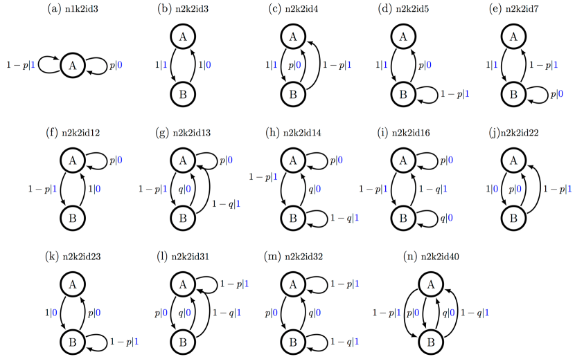
Figure 1: All binary, unifilar hidden Markov model topologies with one or two states. Each topology, designated (a) through (n), also has a unique label that provides the number of states $n=1,2$, the alphabet size $k=2$, and a unique id that comes from the algorithm used to enumerate all possible model topologies [20]. Model edges are labeled with a transition probability and output symbol using the format: probability $|$ symbol.

To start, we offer a nontechnical introduction to structural inference to be clear how we distinguish (i) a process and its inherent structure from (ii) model topology and these from (iii) sampled data series. A process represents all possible behaviors of a system of interest. It is the object of our focus. Saying that we infer structure means we want to find the process’s organization—the internal mechanisms that generate its observed behavior. However, in any empirical setting we only have samples of the process’s behavior in the form of finite data series. A data series necessarily provides an incomplete picture of the process due to the finite nature of the observation. Finally, we use a model or, more precisely, a model topology to express the process’s structure. The model topology—the set of states and transitions, their connections and observed output symbols—explicitly represents the process’s structure. Typically, there are many model topologies that accurately describe the probabilistic structure of a given process. $\epsilon$-Machines are special within the set of accurate models, however, in that they are the model topology that provides the unique and minimal representation of process structure.

To ground this further, let’s graphically survey different model topologies and consider what processes they represent and how they generate finite data samples. Figure 1 shows models with one or two states that generate binary processes—observed behavior is a sequence of $0$s and $1$s. For example, the smallest model topology is shown in Fig. 1(a) and represents the IID binary process. This model generates data by starting in state $A$ and outputs a $0$ with probability $p$ and a $1$ with probability $1-p$, always returning to state $A$.

A more complex model topology, shown in Fig. 1(g), has two states and four edges. In this case, when the model is in state $A$ it generates a $0$ with probability $p$ and returns to state $A$, or it generates a $1$ with probability $1-p$ and moves to state $B$. When in state $B$, a $0$ is generated with probability $q$ and $1$ with probability $1-q$, moving to state $A$ in both cases. If $p\neq q$ this model topology represents a unique, structured process. However, if $p=q$ the probability of generating a $0$ or $1$ does not depend on states $A$ and $B$ and the resulting process is IID. Thus, this model topology with $p=q$ becomes an overly verbose representation of the IID process, which requires only a single state—the topology of Fig. 1(a). This setting of the transition probabilities is an example where a model topology describes the probabilistic behavior of a process, but does not reflect the structure. In fact, the model topology in Fig. 1(g) is not an $\epsilon$-machine when $p=q$. Rather, the process structure is properly represented by Fig. 1(a), which is.

This example and other cases where specific model topologies are not minimal and unique representations of a process’s structure motivate identifying a subclass of model topologies. All model topologies in Fig. 1 are unifilar hidden Markov models (defined shortly). However, the six model topologies with two states and four edges, Fig. 1(g-i, l-n), are not minimal when $p=q$. As with the previous example, they all become overly complex representations of the IID process for this parameter setting. Excluding these uHMMs leaves a subset of topologies called topological $\epsilon$-machines, Fig. 1(a-f,j-k), that are guaranteed to be minimal and unique representations of process structure for any transition probabilities setting, other than $0$ or $1$. Partly to emphasize the role of process structure and partly to simplify technicalities, in this first introduction to BSI we only consider topological $\epsilon$-machines. A sequel lifts this restriction, adapting BSI to work with all $\epsilon$-machines.

In this way, we see how a process’s structure is expressed in model topology and how possible ambiguities arise. This is the forward problem of statistical inference. Now, consider the complementary inverse problem: Given an observed data series, find the model topology that most effectively describes the unknown process structure. In a Bayesian setting, the first step is to identify those model topologies that can generate the observed data. As just discussed, we do this by choosing a specific model topology and start state and attempting to trace the hidden-state path through the model, using the observed symbols to determine the edges to follow. If there is a path for at least one start state, the model topology is a viable candidate. This process is repeated for each model topology in a specified set, such as that displayed in Fig. 1. The procedure that lists, and tests, model topologies in a set of candidates we call enumeration.

To clarify the procedure for tracing hidden-state paths let’s consider a specific example of observed data consisting of the short binary sequence:

$$11101100111101111001~{}.$$ (1)

If tested against each candidate in Fig. 1, eight of the sixteen model topologies are possible: (a, e, g-i, l-n). For example, using Fig. 1(i) and starting in state $A$, the observed data is generated by the hidden-state path:

$$ABABBABBBABABBABABBBA~{}.$$ (2)

One way to describe this path—one that is central to statistical estimation—is to count the number of times each edge in the model was traversed. Using $n(\sigma{x}|\sigma_{0})$ to denote the number of times that symbol ${x}$ is generated using an edge from state $\sigma$ given that the sequence starts in state $\sigma_{0}$, we obtain: $n(A0|A)=0$, $n(A1|A)=7$, $n(B0|A)=6$, and $n(B1|A)=7$, again assuming $\sigma_{0}=A$. Similar paths and sets of edge counts are found for the eight viable topologies cited above. These counts are the basis for estimating a topology’s transition and start-state probabilities. From these, one can then calculate the probability that each model topology produced the observed data series—each candidate’s posterior probability.

By way of outlining what is to follow, let’s formalize the procedure just sketched in terms of the primary goal of estimating candidates’ posterior probabilities. First, Sec. III recapitulates what is known about the space of structured processes, reviewing how they are represented as $\epsilon$-machines and how topological $\epsilon$-machines are exactly enumerated. Then, Sec. IV adapts Bayesian inference methods to this model class, analyzing transition probability and start state estimation for a single, known topology. Next, setting the context for comparing model topologies, it explores the organization of the prior over the set $\bm{\mathcal{M}}$ of candidate models. Section IV closes with a discussion of how to estimate various process statistics from functions of model parameters. Finally, Sec.  V applies BSI to a series of increasingly complex processes: (i) a finite-order Markov process, (ii) an infinite-order Markov process, and, finally, (iii) an infinite-memory process. Each illustrates BSI’s effectiveness by emphasizing its ability to accurately estimate a process’s stored information (statistical complexity $C_{\mu}$) and randomness (Shannon entropy rate $h_{\mu}$).

III Structured Processes

We describe a system of interest in terms of its observed behavior, following the approach of computational mechanics, as reviewed in [15]. Again, a process is the collection of behaviors that the system produces. A process’s probabilistic description is a bi-infinite chain of random variables, denoted by capital letters $\ldots\,{X}_{t-2}\,{X}_{t-1}\,{X}_{t}\,{X}_{t+1}\,{X}_{t+2}\ldots$. A realization is indicated by lowercase letters $\ldots\,{x}_{t-2}\,{x}_{t-1}\,{x}_{t}\,{x}_{t+1}\,{x}_{t+2}\ldots$. We assume the value ${x}_{t}$ belongs to a discrete alphabet $\mathcal{X}$. We work with blocks ${X}_{t:t^{\prime}}={X}_{t}\ldots{X}_{t^{\prime}-1}$, where the first index is inclusive and the second exclusive.

$\epsilon$-Machines were originally defined in terms of prediction, in the so-called history formulation [16, 15]. Given a past realization ${x}_{-\infty:t}=\ldots{x}_{t-2}\,{x}_{t-1}$ and future random variables ${X}_{t:\infty}={X}_{t}\,{X}_{t+1}\ldots$, the conditional distributions $\mathbb{P}(X_{t:\infty}|{x}_{-\infty:t})$ define the predictive equivalence relation over pasts:

$${x}_{-\infty:t}\sim{x}_{-\infty:t^{\prime}}\Leftrightarrow\mathbb{P}(X_{t:\infty}|{x}_{-\infty:t})\!=\!\mathbb{P}(X_{t^{\prime}:\infty}|{x}_{-\infty:t^{\prime}}).$$ (3)

Within the history formulation, a process determines the $\epsilon$-machine topology through $\sim$: The causal states $\bm{\mathcal{S}}$ are its equivalence classes and these, in turn, induce state-transition dynamics [15]. This way of connecting a process and its $\epsilon$-machine influenced previous approaches to structural inference [16, 25, 19].

The $\epsilon$-machine generator formulation, an alternative, was motivated by the problem of synchronization [26, 27]. There, an $\epsilon$-machine topology defines the process that can be generated by it. Recently, the generator and history formulations were proven to be equivalent [28]. Although, the history view is sometimes more intuitive, the generator view is useful in a variety of applications, especially the approach to structural inference developed here.

Following [26, 27, 28], we start with four definitions that delineate the model classes relevant for temporal pattern discovery.

Definition 1.

A finite-state, edge-labeled hidden Markov model (HMM) consists of:

1. A finite set of hidden states $\bm{\mathcal{S}}=\left\{\sigma_{1},\ldots,\sigma_{N}\right\}$.

2. A finite output alphabet $\mathcal{X}$.

3. A set of $N\times N$ symbol-labeled transition matrices $T^{({x})}$, ${x}\in\mathcal{X}$, where $T^{({x})}_{i,j}$ is the probability of transitioning from state $\sigma_{i}$ to state $\sigma_{j}$ and emitting symbol ${x}$. The corresponding overall state-to-state transition matrix is denoted $T=\sum_{{x}\in\mathcal{X}}T^{({x})}$.

Definition 2.

A finite-state, edge-labeled, unifilar HMM (uHMM) is a finite-state, edge-labeled HMM with the following property:

• Unifilarity: For each state $\sigma_{i}\in\bm{\mathcal{S}}$ and each symbol ${x}\in\mathcal{X}$ there is at most one outgoing edge from state $\sigma_{i}$ that outputs symbol ${x}$.

Definition 3.

A finite-state $\epsilon$-machine is a uHMM with the following property:

• Probabilistically distinct states: For each pair of distinct states $\sigma_{k},\sigma_{j}\in\bm{\mathcal{S}}$ there exists some finite word $w={x}_{0}{x}_{1}\ldots{x}_{L-1}$ such that:

  $$\mathbb{P}(w|\sigma_{0}=\sigma_{k})\neq\mathbb{P}(w|\sigma_{0}=\sigma_{j})~{}.$$

Definition 4.

A topological $\epsilon$-machine is a finite-state $\epsilon$-machine where the transition probabilities for leaving each state are equal for all outgoing edges.

These definitions provide a hierarchy in the model topologies to be considered. The most general set (Def. 1) consists of finite-state, edge-labeled HMM topologies with few restrictions. These are similar to models employed in many machine learning and bioinformatics applications; see, e.g., [1]. Using Def. 2, the class of HMMs is further restricted to be unifilar. The inference methods developed here apply to all model topologies in this class, as well as all more restricted subclasses. As a point of reference, Fig. 1 shows all binary, full-alphabet (able to generate both $0$s and $1$s) uHMM topologies with one or two states. If all states in the model are probabilistically distinct, following Def. 3, these model topologies are also valid generator $\epsilon$-machines. Whether a uHMM is also a valid $\epsilon$-machine often depends on the specific transition probabilities for the machine; see Sec. II for an example. This dependence motivates the final restriction to topological $\epsilon$-machines (Def. 4), which are guaranteed to be minimal even if transition probabilities are equal.

Here, we employ the set of topological $\epsilon$-machines for structural inference. Although specific settings of the transition probabilities are used to define the set of allowed model topologies this does not affect the actual inference procedure. For example, in Fig. 1 only (a-f, j-k) are topological $\epsilon$-machines. However, the set of topological $\epsilon$-machines does exclude a variety of model topologies that might be useful for general time-series inference. For example, when Def. 4 is applied, all processes with full support (all words allowed) reduce to a single-state model. However, broadening the class of topologies beyond the set considered here is straightforward and so we address extending the present methods to them in a sequel. The net result emphasizes structure arising from the distribution’s support and guarantees that inferred models can be interpreted as valid $\epsilon$-machines. And, the goal is to present BSI’s essential ideas for one class of structured processes—the topological $\epsilon$-machines.

States	$\epsilon$-Machines
$n$	$F_{n,2}$
1	1
2	7
3	78
4	1,388
5	35,186

Table 1: Size $F_{n,2}$ of the enumerated library of full-alphabet, binary topological $\epsilon$-machines from one to five states. Reproduced with permission from [20].

The set of topological $\epsilon$-machines can be exactly and efficiently enumerated [20], motivating the use of this model class as our first example application of BSI. Table 1 lists the number $F_{n,k}$ of full-alphabet topologies with $n=1,\ldots,5$ states and alphabet size $k=2$. Compare this table with the model topologies in Fig. 1, where all $n=1$ and $n=2$ uHMMs are shown. Only Fig. 1(a-f,j-k) are topological $\epsilon$-machines, accounting for the difference between the eight models in the table above and the fourteen in Fig. 1. For comparison, the library has been enumerated up to eight states, containing approximately $2\times 10^{9}$ distinct topologies. However, for the examples to follow we employ all $36,660$ binary model topologies up to and including five states as the candidate basis for structural inference.

IV Bayesian Inference

Previously, we developed methods for $k$th-order Markov chains to infer models of discrete stochastic processes and coarse-grained continuous chaotic dynamical systems [29, 6]. There, we demonstrated that correct models for in-class data sources could be effectively and parsimoniously estimated. In addition, we showed that the hidden-state nature of out-of-class data sources could be extracted via model comparison between Markov orders as a function of data series length. Notably, we also found that the entropy rate can be accurately estimated, even when out-of-class data was considered.

The following extends the Markov chain methods to the topologically richer model class of unifilar hidden Markov models. The starting point depends on the unifilar nature of the HMM topologies considered here (Def. 2)—transitions from each state have a unique emitted symbol and destination state. As we demonstrated in Sec. II unifilarity also means that, given an assumed start state, an observed data series corresponds to at most one path through the hidden states. The ability to directly connect observed data and hidden-state paths is not possible in the more general class of HMMs (Def. 1) because they can have many, often exponentially many, possible hidden paths for a single observed data series. In contrast, as a result of unifilarity, our analytic methods previously developed for “nonhidden” Markov chains [29] can be applied to infer uHMMs and $\epsilon$-machines by adding a latent (hidden) variable for the unknown start state. We note in passing that for the more general class of HMMs, including nonunifilar topologies, there are two approaches to statistical inference. The first is to convert them to a uHMM (if possible), using mixed states [30, 31]. The second is to use more conventional computational methods, such as Baum-Welch [32].

Setting aside these alternatives for now, we formalize the connection between observed data series and a candidate uHMM topology discussed in Sec. II. We assume that a data series $D_{0:T}={x}_{0}{x}_{1}\ldots{x}_{T-2}{x}_{T-1}$ of length $T$ has been obtained from the process of interest, with ${x}_{t}$ taking values in a discrete alphabet $\mathcal{X}$. When a specific model topology and start state are assumed, a hidden-state sequence corresponding to the observed data can sometimes, but not always, be found. We denote a hidden state at time $t$ as $\sigma_{t}$ and a hidden-state sequence corresponding to $D_{0:T}$ as $S_{0:T+1}=\sigma_{0}\sigma_{1}\ldots\sigma_{T-1}\sigma_{T}$. Note that the state sequence is longer than the observed data series since the start and final states are included. Using this notation, an observed symbol ${x}_{t}$ is emitted when transitioning from state $\sigma_{t}$ to $\sigma_{t+1}$. For example, using the observed data in Eq. (1), a hidden-state path corresponding to Eq. (2) can be obtained by assuming topology Fig. 1(i) and start state $A$.

We can now write out the probability of an observed data series. We assume a stationary uHMM topology $M_{i}$ with a set of hidden states $\sigma_{i}\in\bm{\mathcal{S}}_{i}$. We add the subscript $i$ to make it clear that we are analyzing a set of distinct, enumerated model topologies. As demonstrated in the example from Sec. II, edge counts $n(\sigma_{i}{x}|\sigma_{i,0})$ are obtained by tracing the hidden-state path given an assumed start state $\sigma_{i,0}$. Putting this all together, the probability of observed data $D_{0:T}$ and corresponding state-path $S_{0:T+1}$ is:

$$\mathbb{P}(S_{0:T+1},D_{0:T}) = p(\sigma_{i,0})$$

$$\times \prod_{\sigma_{i}\in\bm{\mathcal{S}}_{i}}\prod_{{x}\in\mathcal{X}}p({x}|\sigma_{i})^{n(\sigma_{i}{x}|\sigma_{i,0})}~{}.$$

A slight manipulation of Eq. (IV) lets us write the probability of observed data and hidden dynamics, given an assumed start state $\sigma_{i,0}$, as:

$$\mathbb{P}(S_{0:T+1},D_{0:T}|\sigma_{i,0})=\prod_{\sigma_{i}\in\bm{\mathcal{S}}_{i}}\prod_{{x}\in\mathcal{X}}p({x}|\sigma_{i})^{n(\sigma_{i}{x}|\sigma_{i,0})}~{}.$$ (5)

The development of Eq. (5) and the simple example provided in Sec. Fig. II lay the groundwork for our application of Bayesian methods. That is, given topology $M_{i}$ and start state $\sigma_{i,0}$, the probability of observed data $D_{0:T}$ and hidden dynamics $S_{0:T+1}$ can be calculated. For the purposes of inference, the combination of observed and hidden sequences is our data $\mathbf{D}=(D_{0:T},S_{0:T+1})$.

IV.1 Inferring Transition Probabilities

The first step is to infer transition probabilities for a single uHMM or topological $\epsilon$-machine $M_{i}$. As noted above, we must assume a start state $\sigma_{i,0}$ so that edge counts $n(\sigma_{i},{x}|\sigma_{i,0})$ can be obtained from $D_{0:T}$. This requirement means that the inferred transition probabilities also depend on the assumed start state. At a later stage, when comparing model topologies, we demonstrate that the uncertainty in start state can be averaged over.

The set $\{\theta_{i}\}$ of parameters to estimate consists of those transition probabilities defined to be neither one nor zero by the assumed topology: $\theta_{i}=\{0<p({x}|\sigma_{i},\sigma_{i,0})<1:\sigma_{i}\in\bm{\mathcal{S}}_{i}^{*},\sigma_{i,0}\in\bm{\mathcal{S}}_{i}\}$, where $\bm{\mathcal{S}}_{i}^{*}\subseteq\bm{\mathcal{S}}_{i}$ is the subset of hidden states with more than one outgoing edge. The resulting likelihood follows directly from Eq. (5):

$$\mathbb{P}(\mathbf{D}|\theta_{i},\sigma_{i,0},M_{i})=\prod_{\sigma_{i}\in\bm{\mathcal{S}}_{i}}\prod_{{x}\in\mathcal{X}}p({x}|\sigma_{i},\sigma_{i,0})^{n(\sigma_{i},{x}|\sigma_{i,0})}~{},$$ (6)

We note that the set of transition probabilities used in the above expression are unknown when doing statistical inference. However, we can still write the probability of the observed data given a setting for these unknown values, as indicated by the notation for the likelihood: $\mathbb{P}(\mathbf{D}|\theta_{i},\sigma_{i,0},M_{i})$. Although not made explicit above, there is also a possibility that the likelihood vanishes for some, or all, start states if the observed data is not compatible with the topology. For example, if we attempt to use Fig. 1(d) for the observed data in Eq. (1) we find that neither $\sigma_{i,0}=A$ nor $\sigma_{i,0}=B$ leads to viable paths for the observed data, resulting in zero likelihood.

For later use, we denote the number of times a hidden state is visited by $n(\sigma_{i}\bullet|\sigma_{i,0})=\sum_{{x}\in\mathcal{X}}n(\sigma_{i},{x}|\sigma_{i,0})$.

Equation (6) exposes the Markov nature of the dynamics on the hidden states and suggests adapting the methods we previously developed for Markov chains [29]. Said simply, states that corresponded there to histories of length $k$ for Markov chain models are replaced by a hidden state $\sigma_{i}$. Mirroring the earlier approach, we employ a conjugate prior for transition probabilities. This choice means that the posterior distribution has the same form as the prior, but with modified parameters. In the present case, the conjugate prior is a product of Dirichlet distributions:

$$\mathbb{P}(\theta_{i}|\sigma_{i,0},M_{i}) = \prod_{\sigma_{i}\in\bm{\mathcal{S}}_{i}^{*}}\Biggl{\{}\frac{\Gamma(\alpha(\sigma_{i}\bullet|\sigma_{i,0}))}{\prod_{{x}\in\mathcal{X}}\Gamma(\alpha(\sigma_{i}{x}|\sigma_{i,0}))}\Biggr{.}$$

$$\times \delta\Biggl{(}1-\sum_{{x}\in\mathcal{X}}p({x}|\sigma_{i},\sigma_{i,0})\Biggr{)}$$

$$\times \Biggl{.}\prod_{{x}\in\mathcal{X}}p({x}|\sigma_{i},\sigma_{i,0})^{\alpha(\sigma_{i}{x}|\sigma_{i,0})-1}\Biggr{\}}~{},$$

where $\alpha(\sigma_{i}\bullet|\sigma_{i,0})=\sum_{{x}\in\mathcal{X}}\alpha(\sigma_{i}{x}|\sigma_{i,0})$. In the examples to follow we take $\alpha(\sigma_{i}{x}|\sigma_{i,0})=1$ for all parameters of the prior. This results in a uniform density over the simplex for all transition probabilities to be inferred, irrespective of start state [33].

The product of Dirichlet distributions includes transition probabilities only from hidden states in $\bm{\mathcal{S}}_{i}^{*}$ because these states have more than one outgoing edge. For transition probabilities from states $\sigma_{i}\not\in\bm{\mathcal{S}}_{i}^{*}$ there is no need for an explicit prior because the transition probability must be zero or one by definition of the uHMM topology. As a result, the prior expectation for transition probabilities is:

$$\bm{E}_{\mbox{prior}}\left[p({x}|\sigma_{i},\sigma_{i,0})\right]=\frac{\alpha(\sigma_{i}{x}|\sigma_{i,0})}{\alpha(\sigma_{i}\bullet|\sigma_{i,0})}~{},$$ (8)

for states $\sigma_{i}\in\bm{\mathcal{S}}_{i}^{*}$.

Next, we employ Bayes’ Theorem to obtain the posterior distribution for the transition probabilities given data and prior assumptions. In this context, it takes the form:

$$\mathbb{P}(\theta_{i}|\mathbf{D},\sigma_{i,0},M_{i})=\frac{\mathbb{P}(\mathbf{D}|\theta_{i},\sigma_{i,0},M_{i})\mathbb{P}(\theta_{i}|\sigma_{i,0},M_{i})}{\mathbb{P}(\mathbf{D}|\sigma_{i,0},M_{i})}~{}.$$ (9)

The terms in the numerator are already specified above as the likelihood and the prior, Eqs. (6) and (IV.1), respectively.

The normalization factor in Eq. (9) is called the evidence, or marginal likelihood. This term integrates the product of the likelihood and prior with respect to the set of transition probabilities $\theta_{i}$:

$$\mathbb{P}(\mathbf{D}|\sigma_{i,0},M_{i}) = \int\,d\theta_{i}\,\mathbb{P}(\mathbf{D}|\theta_{i},\sigma_{i,0},M_{i})\mathbb{P}(\theta_{i}|\sigma_{i,0},M_{i})$$

$$= \prod_{\sigma_{i}\in\bm{\mathcal{S}}_{i}^{*}}\Biggl{\{}\frac{\Gamma(\alpha(\sigma_{i}\bullet|\sigma_{i,0}))}{\prod_{{x}\in\mathcal{X}}\Gamma(\alpha(\sigma_{i}{x}|\sigma_{i,0}))}$$

$$\times \frac{\prod_{{x}\in\mathcal{X}}\Gamma(\alpha(\sigma_{i}{x}|\sigma_{i,0})+n(\sigma_{i}{x}|\sigma_{i,0}))}{\Gamma(\alpha(\sigma_{i}\bullet|\sigma_{i,0})+n(\sigma_{i}\bullet|\sigma_{i,0}))}\Biggr{\}}~{},$$

resulting in the average of the likelihood with respect to the prior. In addition to normalizing the posterior distribution (Eq. (9)), the evidence is important in our subsequent applications of Bayes’ Theorem. In particular, the quantity is central to the model selection to follow and is used to (i) determine the start state given the model and (ii) compare model topologies.

As discussed above, conjugate priors result in a posterior distribution of the same form, with prior parameters modified by observed counts:

$$P(\theta_{i}|\mathbf{D}, \sigma_{i,0},M_{i})$$

$$=\prod_{\sigma_{i}\in\bm{\mathcal{S}}_{i}^{*}}\Biggl{\{}\frac{\Gamma(\alpha(\sigma_{i}\bullet|\sigma_{i,0})+n(\sigma_{i}\bullet|\sigma_{i,0}))}{\prod_{{x}\in\mathcal{X}}\Gamma(\alpha(\sigma_{i}{x}|\sigma_{i,0})+n(\sigma_{i}{x}|\sigma_{i,0}))}\Biggr{.}$$

$$~{}~{}~{}\times\delta\Biggl{(}1-\sum_{{x}\in\mathcal{X}}p({x}|\sigma_{i},\sigma_{i,0})\Biggr{)}$$ (11)

$$~{}~{}~{}\times\Biggl{.}\prod_{{x}\in\mathcal{X}}p({x}|\sigma_{i},\sigma_{i,0})^{\alpha(\sigma_{i}{x}|\sigma_{i,0})+n(\sigma_{i}{x}|\sigma_{i,0})-1}\Biggr{\}}~{}.$$

Comparing Eqs. (IV.1) and (IV.1)—prior and posterior, respectively—shows that the distributions are very similar: $\alpha(\sigma_{i}{x}|\sigma_{i,0})$ (prior only) is replaced by $\alpha(\sigma_{i}{x}|\sigma_{i,0})+n(\sigma_{i}{x}|\sigma_{i,0})$ (prior plus data). Thus, one can immediately write down the posterior mean for the transition probabilities:

$$\bm{E}_{\mbox{post}} \left[p({x}|\sigma_{i},\sigma_{i,0})\right]$$

$$=\frac{\alpha(\sigma_{i}{x}|\sigma_{i,0})+n(\sigma_{i}{x}|\sigma_{i,0})}{\alpha(\sigma_{i}\bullet|\sigma_{i,0})+n(\sigma_{i}\bullet|\sigma_{i,0})}~{},$$ (12)

for states $\sigma_{i}\in\bm{\mathcal{S}}_{i}^{*}$. As with the prior, probabilities for transitions from states $\sigma_{i}\notin\bm{\mathcal{S}}_{i}^{*}$ are zero or one, as defined by the model topology.

Notably, the posterior mean for the transition probabilities does not completely specify our knowledge since the uncertainty, reflected in functions of the posterior’s higher moments, can be large. These moments are available elsewhere [33]. However, using methods detailed below, we employ sampling from the posterior at this level, as well as other inference levels, to capture estimation uncertainty.

IV.2 Inferring Start States

The next task is to calculate the probabilities for each start state given a proposed machine topology and observed data. Although we are not typically interested in the actual start state, introducing this latent variable is necessary to develop the previous section’s analytic methods. And, in any case, another level of Bayes’ Theorem allows us to average over uncertainty in start state to obtain the probability of observed data for the topology, independent of start state.

We begin with the evidence $\mathbb{P}(\mathbf{D}|\sigma_{i,0},M_{i})$ derived in Eq. (IV.1) to estimate transition probabilities. When determining the start state, the evidence (marginal likelihood) from inferring transition probabilities becomes the likelihood for start state estimation. As before, we apply Bayes’ Theorem, this time with unknown start states, instead of unknown transition probabilities:

$$\mathbb{P}(\sigma_{i,0}|\mathbf{D},M_{i})=\frac{\mathbb{P}(\mathbf{D}|\sigma_{i,0},M_{i})\mathbb{P}(\sigma_{i,0}|M_{i})}{\mathbb{P}(\mathbf{D}|M_{i})}~{}.$$ (13)

This calculation requires defining a prior over start states $\mathbb{P}(\sigma_{i,0}|M_{i})$. In practice, setting start states as equally probable a priori is a sensible choice in light of the larger goal of structural inference. The normalization $\mathbb{P}(\mathbf{D}|M_{i})$, or evidence, at this level follows by averaging over the uncertainty in $\sigma_{i,0}$:

$$\mathbb{P}(\mathbf{D}|M_{i})=\sum_{\sigma_{i,0}\in\bm{\mathcal{S}}_{i}}\mathbb{P}(\mathbf{D}|\sigma_{i,0},M_{i})\mathbb{P}(\sigma_{i,0}|M_{i})~{}.$$ (14)

The result of this calculation no longer explicitly depends on start states or transition probabilities. The uncertainty created by these unknowns has been averaged over, producing a very useful quantity for comparing different topologies: $\mathbb{P}(\mathbf{D}|M_{i})$. However, one must not forget that inferring transition and start state probabilities underlies the structural comparisons to follow. In particular, the priors set at the levels of transition probabilities and start states can impact the structures detected due to the hierarchical nature of the inference: $\mathbb{P}(\mathbf{D}|\theta_{i},\sigma_{i,0},M_{i})\rightarrow\mathbb{P}(\mathbf{D}|\sigma_{i,0},M_{i})\rightarrow\mathbb{P}(\mathbf{D}|M_{i})$.

IV.3 Inferring Model Topology

So far, we inferred transition probabilities and start states for a given model topology. Now, we are ready to compare different topologies in a set $\bm{\mathcal{M}}$ of candidate models. As with inferring start states given a topology, we write down yet another version Bayes’ Theorem, except one for model topology:

$$\mathbb{P}(M_{i}|\mathbf{D},\bm{\mathcal{M}})=\frac{\mathbb{P}(\mathbf{D}|M_{i},\bm{\mathcal{M}})\mathbb{P}(M_{i}|\bm{\mathcal{M}})}{\mathbb{P}(\mathbf{D}|\bm{\mathcal{M}})}~{},$$ (15)

writing the likelihood as $\mathbb{P}(\mathbf{D}|M_{i},\bm{\mathcal{M}})$ to make the nature of the conditional distributions clear. This is exactly the same, however, as the evidence derived above in Eq. (14): $\mathbb{P}(\mathbf{D}|M_{i})=\mathbb{P}(\mathbf{D}|M_{i},\bm{\mathcal{M}})$. Equality holds because nothing in calculating the previous evidence term directly depends on the set of models considered. The evidence $\mathbb{P}(\mathbf{D}|\bm{\mathcal{M}})$, or normalization term, in Eq. (15) has the general form:

$$\mathbb{P}(\mathbf{D}|\bm{\mathcal{M}})=\sum_{M_{j}\in\bm{\mathcal{M}}}\mathbb{P}(\mathbf{D}|M_{j},\bm{\mathcal{M}})\mathbb{P}(M_{j}|\bm{\mathcal{M}})~{}.$$ (16)

To apply Eq. (15) we must first provide an explicit prior over model topologies. One general form, tuned by single parameter $\beta$, is:

$$\mathbb{P}(M_{i}|\bm{\mathcal{M}})=\frac{\exp\left(-\beta\phi(M_{i})\right)}{\sum_{M_{j}\in\bm{\mathcal{M}}}\exp\left(-\beta\phi(M_{j})\right)}~{},$$ (17)

where $\phi(M_{i})$ is some desired function of model topology. In the examples to follow we use the number of causal states—$\phi(M_{i})=|M_{i}|$—thereby penalizing for model size. This is particularly important when a short data series is being investigated. However, setting $\beta=0$ removes the penalty, making all models in $\bm{\mathcal{M}}$ a priori equally likely. It is important to investigate the effects of choosing a specific $\beta$ for a given set of candidate topologies. Below, we first demonstrate the effect of choosing $\beta=0$, $2$, or $4$. After that, however, we employ $\beta=4$ since this value, in combination with the set of one- to five-state binary-alphabet topological $\epsilon$-machines, produces a preference for one- and two-state machines for short data series and still allows for inferring larger machines with only a few thousand symbols. Experience with this $\beta$ shows that it is structurally conservative.

In the examples we explore two approaches to using the results of structural inference. The first takes into account all model topologies in the set considered, weighted according to the posterior distribution given in Eq. (15). The second selects a single model $M_{\mbox{map}}$ that is the maximum a posteriori (MAP) topology:

$$M_{\mbox{map}}=\operatorname*{argmax}_{M_{i}\in\bm{\mathcal{M}}}\mathbb{P}(M_{i}|\mathbf{D},\bm{\mathcal{M}})~{}.$$ (18)

The difference between these methods is most dramatic for short data series. Also, using the MAP topology often underestimates the uncertainty in functions of the model parameters; which we discuss shortly. Of course, since one throws away any number of comparable models, estimating uncertainty in any quantity that explicitly depends on the model topology cannot be done properly if MAP selection is employed. However, we expect some will want or need to use a single model topology, so we consider both methods.

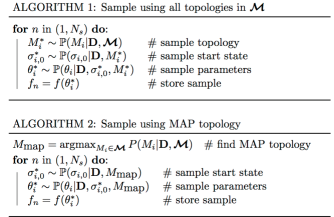
Figure 2: Pseudocode for generating $N_{s}$ samples of a function $f(\theta_{i})$ of model parameters $\{\theta_{i}\}$. Algorithm 1 samples a topology each time through the loop, whereas Algorithm 2 uses the MAP topology for all iterations. The sampling at each stage allows for the creation of a set of samples $\{f_{n}\}$ that accurately reflect the many sources of uncertainty in the posterior distribution.

IV.4 Estimating Functions of Model Parameters

A primary goal in inference is estimating functions that depend on an inferred model’s parameters. We denote this $f(\theta_{i})$ to indicate the dependence on transition probabilities. Unfortunately, substituting the posterior mean for the transition probabilities into some function of interest does not provide the desired expectation. In general, obtaining analytic expressions for the posterior mean of desired functions is quite difficult; see, for example, [34, 35]. Deriving expressions for the uncertainty in the resulting estimates is equally involved and typically not done; although see [34].

Above, the inference method required inferring transition probabilities, start state, and topology. Function estimation, as a result, should take into account all these sources of uncertainty. Instead of deriving analytic expressions for posterior means (if possible), we turn to numerical methods to estimate function means and uncertainties in great detail. We do this by repeatedly sampling from the posterior distribution at each level to obtain a sample $\epsilon$-machine and evaluating the function of interest for the sampled parameter values. The algorithms in Fig. 2 detail the process of sampling $f(\theta_{i})$ using all candidate models $\bm{\mathcal{M}}$ (Algorithm 1) or the single $M_{\mbox{\tiny MAP}}$ model (Algorithm 2). Given a set of samples of the function of interest, any summary statistic can be employed. In the examples, we generate $N_{s}=50,000$ samples from which we estimate a variety of properties. More specifically, these samples are employed to estimate the posterior mean and the 95%, equal-tailed, credible interval (CI) [24]. This means there is a 5% probability of samples being outside the specified interval, with equal probability of being above or below the interval. Finally, a Gaussian kernel density estimation (Gkde) is used to visualize the posterior density for the functions of interest.

The examples demonstrate estimating process randomness and structure from data series using the two algorithms introduced above. For a known $\epsilon$-machine topology $M_{i}$, with specified transition probabilities $\{p({x}|\sigma_{i})\}$, these properties are quantified using the entropy rate $h_{\mu}$ and statistical complexity $C_{\mu}$, respectively. The entropy rate is:

$$h_{\mu}=-\sum_{\sigma_{i}\in\bm{\mathcal{S}}_{i}}p(\sigma_{i})\sum_{{x}\in\mathcal{X}}p({x}|\sigma_{i})\log_{2}p({x}|\sigma_{i})$$ (19)

and the statistical complexity is:

$$C_{\mu}=-\sum_{\sigma_{i}\in\bm{\mathcal{S}}_{i}}p(\sigma_{i})\log_{2}p(\sigma_{i})~{}.$$ (20)

In these expressions, the $p(\sigma_{i})$ are the asymptotic state probabilities determined by the left eigenvector (normalized in probability) of the internal Markov chain transition matrix $T=\sum_{{x}\in\mathcal{X}}T^{(x)}$. Of course, $h_{\mu}$ and $C_{\mu}$ are also functions of the model topology and transition probabilities, so these quantities provide good examples of how to estimate functions of model parameters in general.

V Examples

We divide the examples into two parts. First, we demonstrate inferring transition probabilities and start states for a known topology. Second, we focus on inferring $\epsilon$-machine topology using the set of all binary, one- to five-state topological $\epsilon$-machines, consisting of $36,660$ candidates; see Table 1. We use the convergence of estimates for the information-theoretic values $h_{\mu}$ and $C_{\mu}$ to monitor structure discovery. However, estimating model parameters is at the core of the later examples and so we start with this procedure.

For each example we generate a single data series $D_{0:T}$ of length $T=2^{17}$. When analyzing convergence, we consider subsamples $D_{0:L}$ of lengths $L=2^{i}$, using $i=0,1,2,\ldots,17$. For example, a four-symbol sequence starting at the first data point is designated $D_{0:4}={x}_{0}{x}_{1}{x}_{2}{x}_{3}$. The overlapping analysis of a single data series gives insight into convergence for the inferred models and for the statistics estimated.

V.1 Estimating Parameters

V.1.1 Even Process

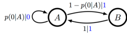
Figure 3: State-transition diagram for the Even Process’s $\epsilon$-machine topology. The “true” value of the unspecified transition probability is $p(0|A)=1/2$. For this topology, $\bm{\mathcal{S}}_{\mbox{even}}=\{A,B\}$ and $\bm{\mathcal{S}}_{\mbox{even}}^{*}=\{A\}$ because state $B$ has only one outgoing transition.

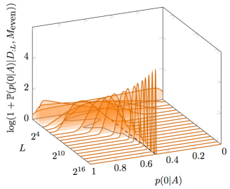
Figure 4: (Color online) Convergence of posterior density $\mathbb{P}(p(0|A)|D_{0:L},M_{\mbox{even}})$ as a function of subsample length $L=2^{i}$, $i=0,1,2,\ldots,17$. Each posterior density plot uses a Gaussian kernel density estimator with $50,000$ samples from the posterior. The true value of $p(0|A)=1/2$ appears as a dashed line and the posterior mean as a solid line.

We first explore a single example of inferring properties of a known data source using Eqs. (6)-(IV.1). We generate a data series from the Even Process and then, using the correct topology (Fig. 3), we infer start states and transition probabilities and estimate the entropy rate and statistical complexity. We do not concentrate on this level of inference in subsequent examples, preferring to focus instead on model topology and its representation of the unknown process structure. Nonetheless, the procedure detailed here underlies all of the examples.

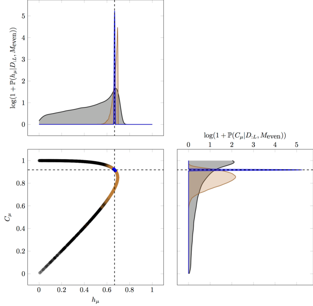
Figure 5: Convergence of randomness ($h_{\mu}$) and structure ($C_{\mu}$) calculated with transition probabilities and start states estimated from Even Process data, assuming the correct topology. $50,000$ samples were taken from the joint posterior $\mathbb{P}(h_{\mu},C_{\mu}|D_{0:L},M_{\mbox{even}})$. (Lower left) A subsample of size $5,000$ for data sizes $L=1$ (black), $L=64$ (brown), and $L=16,384$ (blue). Gaussian kernel density estimates (using all $50,000$ samples) of the marginal distributions $\mathbb{P}(h_{\mu}|D_{0:L},M_{\mbox{even}})$ (top) and $\mathbb{P}(C_{\mu}|D_{0:L},M_{\mbox{even}})$ (right) for the same values of $L$. Dashed lines indicate the true values of $h_{\mu}$ and $C_{\mu}$ for the Even Process.

The Even Process is notable because it has infinite Markov order. This means no finite-order Markov chain can reproduce its word distribution [29]. It can be finitely modeled, though, with a finite-state unifilar HMM—the $\epsilon$-machine of Fig. 3. A single data series was generated using the Even Process $\epsilon$-machine with $p(0|A)=1/2$. The start state was randomized before generating sequence data of length $T=2^{17}$. As it turned out, the initial segment was $D_{0:T}=100\ldots$, indicating that the unknown start state was $B$ on that realization. This is so because the first symbol is a $1$, which can be generated starting in either state $A$ or $B$, but the sequence $10$ is only possible by starting at node $B$.

Next, we estimate the transitions from the generated data series using length-$L$ subsamples $D_{0:L}={x}_{0}{x}_{1}\ldots{x}_{L-1}$ to track convergence. Although the mean and other moments of the Dirichlet posterior can be calculated analytically [33], we sample values using Algorithm 2 in Fig. 2. However, in this example we employ $M_{\mbox{even}}$ instead of $M_{\mbox{map}}$ because we are focused on the model parameters for a known topology. The posterior density for each subsample $D_{0:L}$ is plotted in Fig. 4 using Gaussian kernel density estimation (Gkde). The true value of $p(0|A)$ is shown as a black, dashed line and the posterior mean as a solid, gray line. (Both lines connect values evaluated at each length $L=2^{0},2^{1},\ldots 2^{17}$.) The convergence of the posterior density to the correct value of $p(0|A)=1/2$ with increasing data size is clear and, moreover, the true value is always in a region of positive probability.

For our final example using a known topology we estimate $h_{\mu}$ and $C_{\mu}$ from the Even Process data. This illustrates estimating these functions of model parameters when the $\epsilon$-machine topology is known but there is uncertainty in start state and transition probabilities. As above, we use Algorithm 2 in Fig. 2 and employ the known machine structure. We sample start states and transition probabilities, followed by calculating $h_{\mu}$ and $C_{\mu}$—via Eqs. (19) and (20), respectively—to build a posterior density for these quantities.

Figure 5 presents the joint distribution for $C_{\mu}$ and $h_{\mu}$ along with the Gkde estimation of their marginal densities. Samples from the joint posterior distribution are plotted in the lower left panel for subsample lengths $L=1,64,$ and $16,384$. Only $5,000$ of the available samples are displayed in this panel to minimize the graphic’s size. The marginal densities for $h_{\mu}$ (top panel) and $C_{\mu}$ (right panel) are plotted using a Gkde with all $50,000$ samples. Small data size ($L=1$, indicated by black points) samples allow a wide range of structure and randomness constrained only by the Even Process $\epsilon$-machine topology. The range of $h_{\mu}$ and $C_{\mu}$ reflect the flat priors set for start states and transition probabilities. We note that a uniform prior distribution over transition probabilities and start states does not produce a uniform distribution over $h_{\mu}$ or $C_{\mu}$. Increasing the size of the data subsample to $L=64$ (brown points) results in a considerable reduction in the uncertainty for both functions. For this amount of data, the possible values of entropy rate and statistical complexity curve around the true value in the $h_{\mu}-C_{\mu}$ plane and result in a shifted peak for the marginal density for $h_{\mu}$. For subsample length $L=16,384$ (blue points) the estimates of both functions of model parameters converge to the true values, indicated by the black, dashed lines.

V.2 Inferring Process Structure

We are now ready to demonstrate BSI’s efficacy for structural inference via a series of increasingly complex processes, monitoring convergence using data subsamples up to a length of $L=2^{17}$. In this, we determine the number of hidden states, number of edges connecting them, and symbols output on each transition. As discussed above, we use the set of topological $\epsilon$-machines as candidates because an efficient and exhaustive enumeration is available.

For comparison, we first explore the organization of the prior over the set of candidate $\epsilon$-machines using intrinsic informational coordinates—the process entropy rate $h_{\mu}$ and statistical complexity $C_{\mu}$. We focus on their joint distribution, as induced by various settings of the prior parameter $\beta$. The results lead us to use $\beta=4$ for the subsequent examples. This value creates a preference for small models when little data is available but allows for a larger number of states when reasonable amounts of data support it.

We establish the BSI’s effectiveness by inferring the structure of a finite-order Markov process, an infinite-order Markov process, and an infinite memory process. Again, the proxy for convergence is estimating structure and randomness as a function of the data subsample length $L$. Comparing these quantities’ posterior distributions with their prior illustrates uncertainty reduction as more data is analyzed.

V.2.1 Priors for Structured Processes

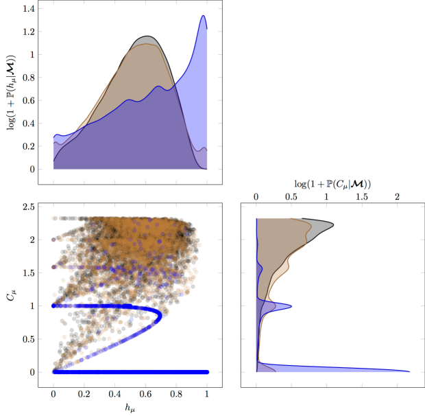
Figure 6: Model prior dependence on penalty parameter $\beta$: $50,000$ samples were taken from the joint prior $\mathbb{P}(h_{\mu},C_{\mu}|\bm{\mathcal{M}})$ using all binary-alphabet, topological $\epsilon$-machines with $1-5$ states and parameters: $\beta=0$ (black), $\beta=2$ (brown), and $\beta=4$ (blue). (Lower left) A subsample of size $5,000$ from the joint distribution is shown for each value of $\beta$. A Gaussian kernel density estimation, using all $50,000$ samples for each value of $\beta$, of the marginal distributions $\mathbb{P}(h_{\mu}|\bm{\mathcal{M}})$ (top) and $\mathbb{P}(C_{\mu}|\bm{\mathcal{M}})$ (right).

Here, we use a prior over all binary-alphabet, topological $\epsilon$-machines with one to five states. (Recall Table 1.) We denote the set of topological $\epsilon$-machines detailed in Table 1 as $\bm{\mathcal{M}}$. Equation (17) allows specifying a preference for smaller $\epsilon$-machines by setting $\beta>0$ and defining the function of model structure to be the number of states: $\phi(M_{i})=|M_{i}|$. Beyond setting this explicitly, there is an inherent bias to smaller models inversely proportional to the parameter space dimension. The parameter space is that of the estimated transition probabilities. Its dimension is the number of states with more than one out-going transition. However, candidate $\epsilon$-machine topologies with many states and few transitions result in a small parameter space and so may be assigned high probability for short data series. In addition, the prior over topologies must take into account the increasing number of candidates as the number of states increases. Setting $\beta$ sufficiently high so that large models are not given high probability under these conditions is reasonable, as we would like to approach structure estimates ($C_{\mu}$) monotonically from below, as data size increases.

Figure 6 plots samples from the resulting joint prior for $(h_{\mu},C_{\mu})$ as well as the corresponding Gkde for marginal densities of both quantities. The data are generated by using the method of Sec. IV.4 and replacing the posterior density with the prior density. Specifically, rather than sampling a topology $M_{i}$ from $\mathbb{P}(M_{i}|D,\bm{\mathcal{M}})$, we sample from $\mathbb{P}(M_{i}|\bm{\mathcal{M}})$. Similar substitutions are made at each level, using the distributions that do not depend on observed data, resulting in samples from the prior. Each color in the figure reflects samples using all $\epsilon$-machines in $\bm{\mathcal{M}}$ with different values for the prior parameter: $\beta=0$ (black), $\beta=2$ (brown) and $\beta=4$ (blue). While $\beta=0$ has many samples at high $C_{\mu}$, reflecting the large number of five-state $\epsilon$-machines, increasing to $\beta=2$ results in noticeable bands in the $h_{\mu}-C_{\mu}$ plane and peaks at $C_{\mu}=\log_{2}1$, $C_{\mu}=\log_{2}2$, $C_{\mu}=\log_{2}3$ bits, and so on. This reflects the fact that larger $\beta$ makes smaller machines more likely. As a consequence, the emergence of patterns due to one-, two-, and three-state topologies is seen. Setting $\beta=4$ shows a stronger a priori preference for one- and two-state machines, reflected by the strong peaks at $C_{\mu}=0$ bits and $C_{\mu}=1$ bit. Interestingly, the prior distribution over $h_{\mu}$ and $C_{\mu}$ is quite similar for $\beta=0$ and $2$, with more distributional structure due to smaller $\epsilon$-machines at $\beta=2$. However, the prior distribution for $h_{\mu}$ and $C_{\mu}$ is quite different for $\beta=4$, creating a strong preference for one- and two-state topologies. This results in an a priori preference for low $C_{\mu}$ and high $h_{\mu}$ that, as we demonstrate shortly, is modified for moderate amounts of data. We employ $\beta=4$ as a reasonable value in all subsequent examples. In practice, sensitivity to this choice should be tested in each application to verify that the resulting behavior is appropriate. We suggest small, nonzero values as reasonable starting points. As always, sufficient data makes the choice relatively unimportant for the resulting inference.

V.2.2 Markov Example: The Golden Mean Process

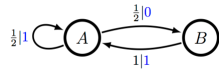
Figure 7: Golden Mean Process’s $\epsilon$-machine.

The first example of structural inference explores the Golden Mean Process, pictured in Fig. 7. Although it is illustrated as an HMM in the figure, it is effectively a Markov chain with no hidden states: observing a $1$ corresponds to state $A$, whereas observing $0$ means the process is in state $B$. Previously, we showed that this data source can be inferred using the model class of $k$th order Markov chains, as expected [29]. However, the Golden Mean Process is also a member of the class of binary-alphabet, topological $\epsilon$-machines considered here. As a result, structural inference from Golden Mean data is an example of in-class modeling.

We proceed using the approach laid out above for the Even Process transition probabilities and start states. We generated a single data series by randomizing the start state and creating a symbol sequence of length $T=2^{17}$ using the Golden Mean Process $\epsilon$-machine. As above, we monitor the convergence using subsamples $D_{0:L}=x_{0}x_{1}\ldots x_{L-1}$ for lengths $L=2^{i}$, $i=0,1,\ldots 17$. The candidate machines $\bm{\mathcal{M}}$ consist of all $36,600$ $\epsilon$-machine topologies in Table 1. Estimating $h_{\mu}$ and $C_{\mu}$ aids in monitoring convergence of inferred topology and related properties to the correct values. In addition, we provide supplementary tables and figures, using both $\bm{\mathcal{M}}$ and the maximum a posteriori model $M_{\mbox{\tiny MAP}}$ at each data length $L$, to give a detailed view of structural inference.

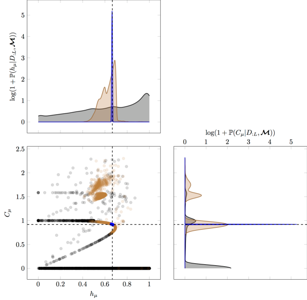
Figure 8: Convergence of randomness ($h_{\mu}$) and structure ($C_{\mu}$) calculated with model topologies, transition probabilities, and start states estimated from Golden Mean Process data, using all one- to five-state topological $\epsilon$-machines. $50,000$ samples were taken from the joint posterior distribution $\mathbb{P}(h_{\mu},C_{\mu}|D_{0:L},\bm{\mathcal{M}})$. (Lower left) Subsample of size $5,000$ for data sizes $L=1$ (black), $L=64$ (brown), and $L=16,384$ (blue). Gaussian kernel density estimates of the marginal distributions (using all $50,000$ samples) $\mathbb{P}(h_{\mu}|D_{0:L},\bm{\mathcal{M}})$ (top) and $\mathbb{P}(C_{\mu}|D_{:L},\bm{\mathcal{M}})$ (right) for the same values of $L$. Dashed lines indicate the true values of $h_{\mu}$ and $C_{\mu}$ for the Golden Mean Process.

Figure 8 plots samples from the joint posterior over $(h_{\mu},C_{\mu})$, as well as their marginal distributions, for three subsample lengths. As in Fig. 5, we consider $L=1$ (black), $L=64$ (brown), and $L=16,384$ (blue). However, this example employs the full set $\bm{\mathcal{M}}$ of candidate topologies. For small data size ($L=1$) the distribution closely approximates the prior distribution for $\beta=4$, as it should. At data size $L=64$, the samples of both the $h_{\mu}$ and $C_{\mu}$ are still broad, resulting in multimodal behavior with considerable weight given to both two- and three-state topologies. Consulting Table S2 in the supplementary material, we see that this is the shortest length that selects the correct topology for the Golden Mean Process (denoted n2k2id5 in Table S2). For smaller $L$, the single-state, two-edge topology is preferred (denoted n1k2id3). However, the probability of the correct model is only 78.7%, leaving a substantial probability for alternative candidates. The uncertainty is further reflected in the large credible interval for $C_{\mu}$ provided by the complete set of models $\bm{\mathcal{M}}$ (see Table S1), ranging from $0.8235$ bits as the lower bound to $1.797$ bits as the upper bound. However, by subsample length $L=16,384$ the probability of the correct topology is 99.998%, given the set of candidate machines $\bm{\mathcal{M}}$, and estimates of both $h_{\mu}$ and $C_{\mu}$ have converged to accurately reflect the correct values.

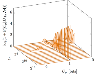
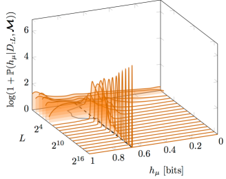
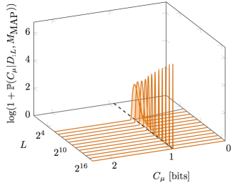
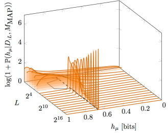
Figure S1: Golden Mean Process, $\beta=4$: Convergence of the posterior densities for $C_{\mu}$ (top) and $h_{\mu}$ (bottom) as a function of subsample length $L$ using the set of all topological $\epsilon$-machines with 1-5 states $\bm{\mathcal{M}}$ (left column) and the maximum a posteriori model $M_{\mbox{MAP}}$ (right column). In each panel, the black, dashed line indicates the true value and the gray, solid line shows the posterior mean.

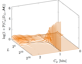
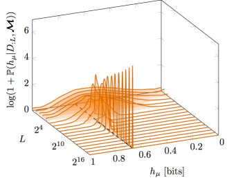
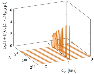
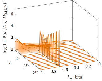
Figure S2: Golden Mean Process, $\beta=2$: Convergence of the posterior densities for $C_{\mu}$ (top) and $h_{\mu}$ (bottom) as a function of subsample length $L$ using the set of all topological $\epsilon$-machines with 1-5 states $\bm{\mathcal{M}}$ (left column) and the maximum a posteriori model $M_{\mbox{MAP}}$ (right column). In each panel, the black, dashed line indicates the true value and the gray, solid line shows the posterior mean. Contrast these panels with those in Figure S1, where the penalty for structure is higher.

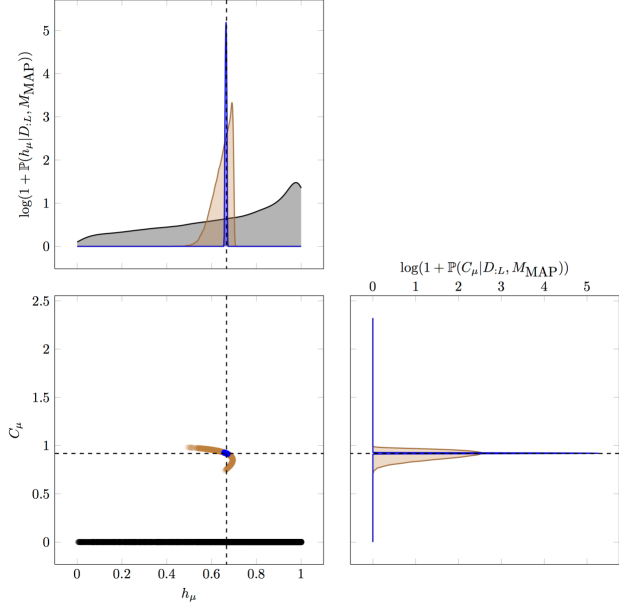
Figure S3: Golden Mean Process: Joint distribution samples using the MAP model at the given lengths instead of the full set of candidate models. Colors correspond to data subsample length, as in previous plots. The MAP topology for $L=1$ (black) has one state and $C_{\mu}=0$, as indicated by the samples in the $h_{\mu}-C_{\mu}$ plane. No Gkde approximation of these samples is provided due to this complete lack of variation.

In addition to Tables S1 and S2, the supplementary materials provide Fig. S1 showing the Gkde estimates of both $h_{\mu}$ and $C_{\mu}$ using $\bm{\mathcal{M}}$ and $M_{\mbox{\tiny MAP}}$ as a function of subsample length. The four panels clearly show the convergence of estimates to the correct values as $L$ increases. For long data series, there is little difference between the inference made using the maximum a posteriori (MAP) model and the posterior over the entire candidate set. However, this is not true for short time series, where using the full set more accurately captures the uncertainty in estimation of the information-theoretic quantities of interest. We note that the $C_{\mu}$ estimates approach the true value from below, preferring small topologies when there is little data and selecting the correct, larger topology only as available data increases. This desired behavior results from setting $\beta=4$ for the prior over $\bm{\mathcal{M}}$. Setting $\beta=2$, shown in Fig. S2, does not have this effect. This value of $\beta$ is insufficient to overcome the large number of three-, four-, and five-state $\epsilon$-machines. Finally, Fig. S3 plots samples from the joint posterior of $h_{\mu}$ and $C_{\mu}$ using only the MAP model for subsample lengths $L=1,64$, and $16,384$. This should be compared with Fig. 8 where the complete set $\bm{\mathcal{M}}$ is used. Again, there is a substantial difference for short data series and much in common for larger $L$.

Before moving to the next example, let’s briefly return to consider start-state inference. The data series generated to test inferring the Golden Mean Process started with the sequence $D_{0:T}=1110\ldots$. We note that the correct start state, which happens to be state $A$ in that realization, cannot be inferred and has lower probability than state $B$ due to the process’s structure: $\mathbb{P}(\sigma_{\mbox{gm},0}=A|D_{0:T}=1110\ldots,M_{\mbox{gm}})\approx 0.3328$ using Eq. (13). The reason for the inability to discern the start state is straightforward. Consulting Fig. 7, we can see that the string $1110$ can be produced beginning in both states $A$ and $B$. On the one hand, assuming $\sigma_{\mbox{gm},0}=A$, the state path would be $AAAAB$ with probability $p(1|A)^{3}p(0|A)=(1/2)^{4}$. On the other hand, assuming $\sigma_{\mbox{gm},0}=B$, the state path is $BAAAB$ with probability $p(1|B)p(1|A)^{2}p(0|A)=1\times(1/2)^{3}$. The only difference in the probabilities is a factor of $p(1|A)=1/2$ versus $p(1|B)=1$ resulting in:

$$\mathbb{P}(\sigma_{i,0}=A|D=1110,M_{\mbox{gm}}) = \frac{(1/2)^{4}}{(1/2)^{4}+(1/2)^{3}}$$

$$= 1/3.$$

This calculation agrees nicely with the result stated above, using finite data and the inference calculations from Eq. (13).

It turns out that any observed data series from the Golden Mean Process that begins with a $1$ will have this ambiguity in start state. However, observed sequences that begin with a $0$ uniquely identify $A$ as the start state since a $0$ is not allowed leaving state $B$. Despite this, the correct topology is inferred and accurate estimates of $h_{\mu}$ and $C_{\mu}$ are obtained.

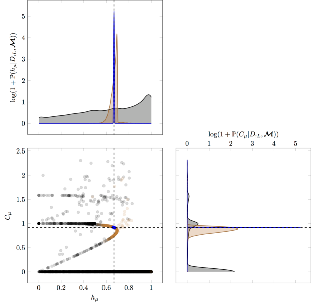
Figure 9: Convergence of randomness ($h_{\mu}$) and structure ($C_{\mu}$) calculated with model topologies, transition probabilities, and start states estimated from Even Process data, using all one- to five-state topological $\epsilon$-machines. $50,000$ samples from the joint posterior $\mathbb{P}(h_{\mu},C_{\mu}|D_{:L},\bm{\mathcal{M}})$. (Lower left) A subsample of $5,000$ for data sizes $L=1$ (black), $L=64$ (brown), and $L=16,384$ (blue). Gaussian kernel density estimates of the marginal distributions (using all $50,000$ samples) $\mathbb{P}(h_{\mu}|D_{:L},\bm{\mathcal{M}})$ (top) and $\mathbb{P}(C_{\mu}|D_{0:L},\bm{\mathcal{M}})$ (right) are shown for the same values of $L$. Dashed lines indicate the true values of $h_{\mu}$ and $C_{\mu}$ for the Even Process.

V.2.3 Infinite-order Markov Example: The Even Process

Next, we consider inferring the structure of the Even Process using the same set of binary-alphabet, one- to five-state, topological $\epsilon$-machines. To be clear, this example differs from Sec. V.1.1, where the correct topology was assumed. Now, we explore Even Process structure using $\bm{\mathcal{M}}$. As noted above, the Even Process is an infinite-order Markov process and inference requires the set of topological $\epsilon$-machines considered here. (However, see out-of-class inference of the Even Process using $k$th-order Markov chains in [29].) As a result, this is an example of in-class inference since the Even Process topology is contained within the set $\bm{\mathcal{M}}$. As with the previous example, a single data series was generated from the Even Process.

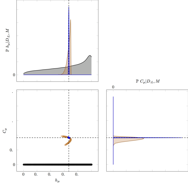
Figure S6: Even Process: Samples of the joint distribution using the MAP model at the given lengths instead of the full set of candidate models. Colors correspond to data subsample length, as in previous plots. The MAP topology for $L=1$ (black) has one state and $C_{\mu}=0$, as indicated by the samples in the $h_{\mu}-C_{\mu}$ plane. No Gkde approximation of these samples is provided due to this complete lack of variation.

Figure 9 shows samples from the posterior distribution over $(h_{\mu},C_{\mu})$ using three subsample lengths $L=1,64$, and $16,384$ as before. An equivalent plot using only the MAP model is provided in the supplementary materials for comparison; see Fig. S6. Again, for short data series the samples mirror the prior distribution as they should. (See black points for $L=1$.) At subsample length $L=64$ the values of $h_{\mu}$ and $C_{\mu}$ are much more tightly delineated. Comparing samples for the Golden Mean Process in Fig. 8 shows that there is much less uncertainty in structure for the Even Process at this data size. Consulting Table S4, the MAP topology for this value of $L$ already identifies the correct topology (denoted n2k2id7) and assigns a probability of 99.41%. This high probability is reflected by the smaller spread, when compared with the Golden Mean example, of the samples of $h_{\mu}$ and $C_{\mu}$. At subsample length $L=16,384$ the probability of the correct topology has grown to 99.998%. Estimates of both $h_{\mu}$ and $C_{\mu}$ are also very accurate, with small uncertainties, at this $L$; see Table S3.

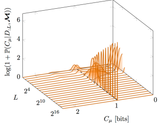
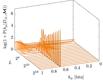
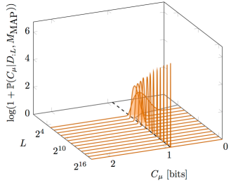
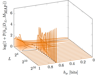
Figure S4: Even Process, $\beta=4$: Convergence of the posterior densities for $C_{\mu}$ (top) and $h_{\mu}$ (bottom) as a function of subsample length $L$ using the set of all topological $\epsilon$-machines with one- to five-states $\bm{\mathcal{M}}$ (left column) and the maximum a posteriori model $M_{\mbox{MAP}}$ (right column). In each panel, the black, dashed line indicates the true value and the gray, solid line shows the posterior mean.

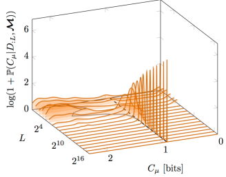
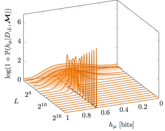
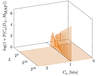
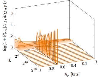
Figure S5: Even Process, $\beta=2$: Convergence of the posterior densities for $C_{\mu}$ (top) and $h_{\mu}$ (bottom) as a function of subsample length $L$ using the set of all topological $\epsilon$-machines with one- to five-states $\bm{\mathcal{M}}$ (left column) and the maximum a posteriori model $M_{\mbox{MAP}}$ (right column). In each panel, the black, dashed line indicates the true value and the gray, solid line shows the posterior mean.

The supplementary materials provide Figs. S4 and S5 to show the convergence of the posterior densities for $h_{\mu}$ and $C_{\mu}$ as a function of subsample length. Figure S4 shows estimates using both $\bm{\mathcal{M}}$ and $M_{\mbox{\tiny MAP}}$ for $\beta=4$. Whereas, Fig. S5 demonstrates the effects of using a small penalty ($\beta=2$) for model size. As seen with the Golden Mean Process, the difference is most apparent at small data sizes. At large $L$, the difference between using the complete set $\bm{\mathcal{M}}$ of models versus the MAP model is minor, as is the effect of choosing $\beta=4$ or $\beta=2$. However, at small data sizes the choices impact the resulting inference. In particular, the choice of $\beta=4$ allows the inference machinery to approach the correct $C_{\mu}$ from below whereas the choice of $\beta=2$ approaches $C_{\mu}$ from above; see Figs. S4 and S5. This behavior, which we believe is desirable, is similar to the inference dynamics observed for the Golden Mean Process, further strengthening the apparent suitability of using $\beta=4$.

Unlike the previous example, the start state for the correct structure is inferred with little data. In this example, the data series begins with the symbols $D_{0:T}=10\ldots$, which can only be generated from state $B$. So, at $L=2$ the start state for the correct topology is determined, but it takes more data—$32$ symbols in this case—for this structure to become the most probable in the set considered.

V.2.4 Out-of-Class Structural Inference: The Simple Nonunifilar Source

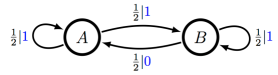
Figure 10: The Simple Nonunifilar Source.

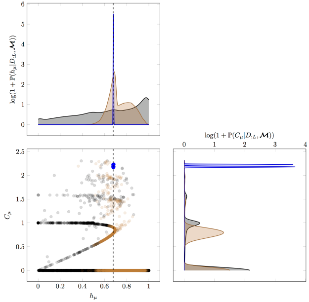
Figure 11: Convergence of randomness ($h_{\mu}$) and structure ($C_{\mu}$) calculated with model topologies, transition probabilities, and start states estimated from Simple Nonunifilar Source data, using all one- to five-state topological $\epsilon$-machines. Sample sizes, colors and line types mirror those in previous figures.

The Simple Nonunifilar Source (SNS) is our final and most challenging example of structural inference due its being out-of-class. The SNS is not only infinite-order Markov, any unifilar presentation requires a infinite number of states. In particular, its $\epsilon$-machine, the minimal unifilar presentation, has a countable infinity of causal states [36]. We can see the difference between the SNS and previous processes by inspecting state $A$, where both out-going edges emit a symbol ‘1’. (See Fig. 10 for a hidden Markov model presentation that is not an $\epsilon$-machine.) This makes the SNS a nonunifilar topology, as the name suggests. Importantly, even if we assume a start state, there is no longer a single, unique path through the hidden states for an observed output data series. This is completely different from the unifilar examples previously considered, where an assumed start state and observed data series either determined a unique path through hidden states or was disallowed. As a result, the inference tools developed here cannot use the HMM topology of Fig. 10. Concretely, this class of representation breaks our method for counting transitions.

Our goal, though, is to use the set of unifilar, topological $\epsilon$-machines at our disposal to infer properties of the Simple Nonunifilar Source. (One reason to do this is that unifilar models are required to calculate $h_{\mu}$.) Typical data series generated by the SNS model are accepted by many of the unifilar topologies in $\bm{\mathcal{M}}$ and a posterior distribution over these models can be calculated. As with previous examples, we demonstrate estimating $h_{\mu}$ and $C_{\mu}$ for the data source. Due to the nonunifilar nature of the source, we expect $C_{\mu}$ estimates to increase with the size of the available data series. However, the ability to estimate $h_{\mu}$ accurately is unclear a priori. Of course, in this example we cannot find the correct model topology because infinite structures are not contained in $\bm{\mathcal{M}}$.

Figure 11 presents the joint posterior for $(h_{\mu},C_{\mu})$ for three subsample lengths. As previously, a single data series of length $2^{17}$ is generated using the SNS and analysis of subsamples $D_{0:L}$ are employed to demonstrate convergence. The short subsample (L=1, black points) is predictably uninteresting, reflecting the the prior distribution over models. For subsamples shorter than $L=64$ the MAP model is the single-state, two-edge topology. (Denoted n1k2id3 in Table S6.) At $L=64$ the Golden Mean Process topology becomes most probable with a posterior probability of 53.01%. The probability of the single-state topology is still 43.98%, though, resulting in $C_{\mu}$’s strongly bimodal marginal posterior observed for $L=64$. (See Fig. 11 brown points, right panel.) Bimodality also appears in the marginal posterior for $h_{\mu}$, with the largest peak coming from the two-state topology and the high entropy rates being contributed by the single-state model. At large data size ($L=16,384$, blue points) $h_{\mu}$ has converged on the true value, while $C_{\mu}$ has sharp, bimodal peaks due to many nearly equally probable five-state topologies. Consulting Table S6, we see that the MAP structure for this value of $L$ has five states (denoted n5k2id22979, there) and a low posterior probability of only 8.63%. Further investigation reveals that there are four additional $\epsilon$-machine topologies (making a total of five) with similar posterior probability. These general details persist for longer subsamples sequences including the complete data series at length $2^{17}$. Although estimating $h_{\mu}$ converges smoothly, the inference of structure as reflected by $C_{\mu}$ does not show signs of graceful convergence.

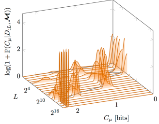
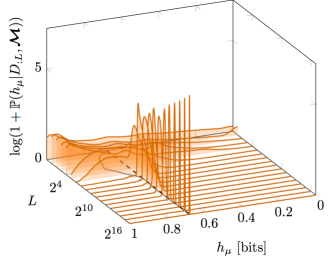
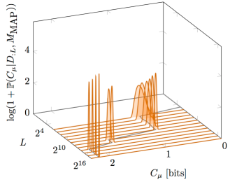
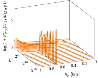
Figure S7: Simple Nonunifilar Source, $\beta=4$: Convergence of the posterior densities for $C_{\mu}$ (top) and $h_{\mu}$ (bottom) as a function of subsample length $L$ using the set of all topological $\epsilon$-machines with one- to five-states $\bm{\mathcal{M}}$ (left column) and the maximum a posteriori model $M_{\mbox{MAP}}$ (right column). In each panel, the black, dashed line indicates the true value and the gray, solid line shows the posterior mean.

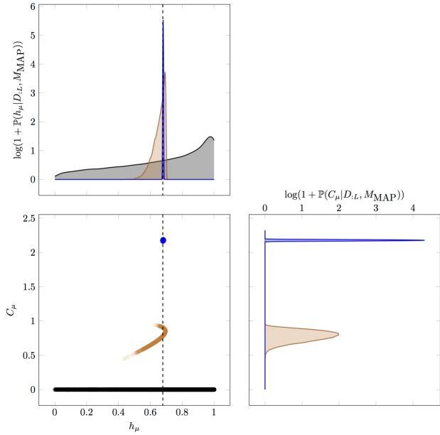
Figure S9: Simple Nonunifilar Source: Joint distribution samples using the MAP model at the given lengths instead of the full set of candidate models. Colors correspond to data subsample length, as in previous plots. The MAP topology for $L=1$ (black) has one state and $C_{\mu}=0$, as indicated by the samples in the $h_{\mu}-C_{\mu}$ plane. No Gkde approximation of these samples is provided due to this complete lack of variation.

We provide supplementary plots in Figs. S7 and S8 that show the convergence of $h_{\mu}$ and $C_{\mu}$ using $\bm{\mathcal{M}}$ and $M_{\mbox{\tiny MAP}}$ for prior parameters $\beta=4$ and $\beta=2$, respectively. Again, the choice of $\beta$ matters most at small data sizes. While the $C_{\mu}$ estimate increases as function of $L$ for $\beta=4$, the use of $\beta=2$ results in posterior means for $C_{\mu}$ that first decrease as function of $L$, then increase. Again, this supports the use of $\beta=4$ for this set of binary-alphabet, topological $\epsilon$-machines. The need to employ the complete model set $\bm{\mathcal{M}}$ versus the MAP topology is most evident at small data sizes; as was also seen in previous examples. However, the $C_{\mu}$ inference in this example is more complicated due to the large number of five-state topologies with roughly equal probability. The MAP method selects just one model, of course, and so cannot represent the posterior distribution’s bimodal behavior. Given that the data source is out-of-class, this trouble is perhaps not surprising. Figure S9 shows samples from the joint posterior of $(h_{\mu},C_{\mu})$ using only the MAP topology. Using the latter also suffers from requiring one to select a single exemplar topology for a posterior distribution that is simply not well represented by a single $\epsilon$-machine.

VI Discussion

The examples demonstrated structural inference of unifilar hidden Markov models using the set of one- to five-state, binary-alphabet, topological $\epsilon$-machines. We found that in-class examples, including the Golden Mean and Even Processes, were effectively and efficiently discovered. That is, the correct topology was accorded the largest posterior probability and estimates of information coordinates $h_{\mu}$ and $C_{\mu}$ were accurate. However, we found that a sufficiently large value of $\beta$, providing the model size penalty, was key to a conservative structural inference. Conservative means that $C_{\mu}$ estimates approach the true value from below, effectively counteracting the increasing number of topologies with larger state sets. For the out-of-class example, given by the Simple Nonunifilar Source, these broader patterns held true. However, structure could not be captured as reflected in the increasing number of states inferred as a function of data length. Also, many topologies had relevant posterior probability for the SNS data, reflecting a lack of consensus and a large degeneracy with regard to structure. This resulted in a multimodal posterior distribution for $C_{\mu}$ and a MAP model with very low posterior probability.

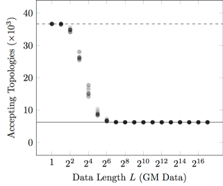
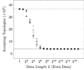
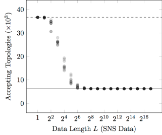
Figure S10: Number of accepting topologies for each of example processes as a function of subsample length $L$. For each, a set of ten data series was created and subsamples of length $L$ were analyzed to determined the number of binary-alphabet, one- to five-state topological $\epsilon$-machines that had at least one valid path for that length. (This would result in nonzero likelihood and posterior probability.) For each data series, a gray point is plotted. Overlapping gray points, created by multiple data series with the same number of accepting topologies at the given value of $L$ generate a darker gray or black point. The horizontal lines indicate the total number of candidate structures ($36,000$, gray dashed line) and the asymptotic number of accepting topologies (solid, gray line). For the Even Process (bottom, left panel), $3,813$ topologies were asymptotically accepting whereas the Golden Mean Process (top, left panel) and Simple Nonunifilar Source (top, right panel) both had $6,225$.

One of the surprises was the number of accepting topologies for a given data set. By this we mean the number of candidate structures for which the data series of interest had a valid path through hidden states, resulting in nonzero posterior probability. In many ways, this aspect of structural inference mirrors grammatical inference for deterministic finite automaton (DFA) [37, 38]. In the supplementary material we provide plots for the three processes considered above showing the number of accepting topologies in the set of one- to five-state $\epsilon$-machines used for $\bm{\mathcal{M}}$. (See Supplemental Fig. S10.) For all of these topologies, a rapid decline in the number of accepting topologies occurs for the first $2^{6}$ to $2^{7}$ symbols, followed by a plateau at a set of accepting topologies. For smaller topologies, which come from the model class under consideration, this pattern makes sense. Often, the smaller topology is embedded within a larger set of states, some of which are never used. For out-of-class examples like the SNS this behavior is less transparent. The rejection of a data series by a given topology provides a first level of filtering by assigning zero posterior probability to the structure due to vanishing likelihood of the data given the model. For the examples given above, of the $36,660$ possible topologies, $6,225$ accepted Golden Mean data, $3,813$ topologies accepted Even Process data, and $6,225$ accepted SNS data when the full data series was considered.

In all of the examples the data sources were stationary, so that statistics did not change over the course of the data series. This is important because stationarity is built into the model class definition employed: the model topology and transition probabilities did not depend on time. However, given a general data series with unknown properties, it is unwise to assume stationarity holds. How can this be probed? One method is to subdivide the data into overlapping segments of equal length. Given these, inference using $\bm{\mathcal{M}}$ or $M_{\mbox{\tiny MAP}}$ should return similar results for each segment. For in-class data sources like the Even and Golden Mean Processes, the true model should be returned for each data subsegment. For out-of-class, but stationary models like the Simple Nonunifilar Source, the true topology cannot be returned, but a consistent model within $\bm{\mathcal{M}}$ should be returned for each data segment.

However, one form of relatively simple nonstationarity—a structural change-point problem such as switching between the Golden Mean and Even Processes—can be detected by BSI applied to subsegments. The inferred topology for early segments returns the Golden Mean topology and later segments return the Even topology. Notably, the inferred topology using all of the data or a subsegment overlapping the switch returns a more complicated model topology reflecting both structures. Of course, detection of this behavior requires sufficient data and slow switching between data sources.

In a sequel we compare BSI to alternative structural inference methods. The range of and differences with these is large and so a comparison demands its own venue. Also, the sequel addresses expanding the model candidates beyond the set of topological $\epsilon$-machines to the full set of unifilar hidden Markov models. A necessary step before useful comparisons can be explored.

VII Conclusion

We demonstrated effective and efficient inference of topological $\epsilon$-machines using a library of candidate structures and the tools of Bayesian inference. Several avenues for further development are immediately obvious. First, as just noted, using full unrestricted $\epsilon$-machines—allowing models outside the set of topological $\epsilon$-machines—is straightforward. This will provide a broad array of candidates within the more general class of unifilar hidden Markov models. In the present setting, by way of contrast, processes with full support (all words allowed) can map only to the single-state topology. Second, refining the eminently parallelizable Bayesian Structural Inference algorithms will allow them to take advantage of large compute clusters and cloud computing to dramatically expand the number of candidate topologies considered. For comparison, the current implementation uses nonoptimized Python on a single thread. This configuration (running on contemporary Linux compute node) takes between $0.6$ and $1.6$ hours, depending on the number of accepting topologies, to calculate the posterior distribution over the $36,660$ candidates for a data series of length $2^{17}$. An additional $10$ to $20$ minutes is needed to generate the $50,000$ samples from the posterior to estimate functions of model parameters, like $h_{\mu}$ and $C_{\mu}$.

We note that the methods of Bayesian Structural Inference can be applied to any set of unifilar hidden Markov models and, moreover, they do not have to employ a large, enumerated library. For example, a small set of candidate fifty-state topologies could be compared for a given data series. This ability opens the door to automated methods for generating candidate structures. Of course, as always, one must keep in mind that all inferences are then conditioned on the, possibly limited or inappropriate, set of model topologies chosen.

Finally, let’s return to the scientific and engineering problem areas cited in the introduction that motivated structural inference in the first place. Generally, Bayesian Structural Inference will find application in fields, such as those mentioned, that rely on finite-order Markov chains or the broader class of (nonunifilar) hidden Markov models. It will also find application in areas requiring accurate estimates of various system statistics. The model class considered here ($\epsilon$-machines) consists of a novel set of topologies and usefully allows one to estimate both randomness and structure using $h_{\mu}$ and $C_{\mu}$. Two of the most basic informational measures. As a result, we expect Bayesian Structural Inference to find an array of applications in bioinformatics, linguistics, and dynamical systems.

Appendix A Overview

The supplementary materials provide tables and figures that lend an in-depth picture of the Bayesian Structural Inference examples. Unless otherwise noted, all analyses presented here use the same single data series and parameter settings detailed in the main text. Please use the main text as the primary guide.

The first three sections address the Golden Mean, Even, and SNS processes. Each provides a table of estimates of $h_{\mu}$ and $C_{\mu}$ using the complete set $\bm{\mathcal{M}}$ of one- to five-state $\epsilon$-machines denoted. Estimates are given for each subsample length $L=2^{i}$, where $i=0,1,2,\ldots,17$, as in the main text. To be clear, this means that we analyze subsamples $D_{0:L}=x_{0}x_{1}x_{2}\ldots x_{L-1}$ using different initial segments of a single long data series, allowing for a consistent view of estimate convergence. For both information-theoretic quantities, we list the posterior mean and equal-tailed, 95% credible interval (CI) constructed using the 2.5% and 97.5% quantiles estimated from $50,000$ samples of the posterior distribution. The CI is denoted by parenthesized number pairs. A second table provides the same estimates of $h_{\mu}$ and $C_{\mu}$ using only the $M_{\tiny\mbox{MAP}}$ model. As a result, this table no longer reflects uncertainty in model topology, which may be small or large depending on the data and subsample length under consideration. An additional column in this second table provides the MAP topology along with its posterior probability. The latter is denoted in parentheses.

In addition to the tables of estimates, figures demonstrate the convergence of $h_{\mu}$ and $C_{\mu}$ marginal posterior distributions as a function subsample length $L$. In this, we consider the difference between posteriors using the complete set $\bm{\mathcal{M}}$ of candidate models and those that only employ the MAP topology. This set of figures also illustrates the difference between $\beta=4$ and $\beta=2$. (We use different data, but still a single time series, for the $\beta=2$ example.) In all plots the marginal posterior distribution for the quantity of interest is estimated using a Gaussian kernel density estimation (Gkde) of the density using $50,000$ samples from the appropriate density. If there is little or no variation in the samples the Gkde fails and no density is drawn. This happens, for example, when the MAP topology has one state, and $C_{\mu}=0$, for small data sizes. Posterior samples are valid, however, and posterior mean and credible interval can be provided (see tables).

Section E plots the number of accepting topologies as a function of subsample length for each of the example data sources in Fig. S10. The panels demonstrate that there are many valid candidate topologies for a given data series, even when subsamples of considerable length are available.

Finally, Sec. F illustrates all topologies that met the MAP criterion for the data sources considered. Notably, there are not many structures to consider despite the large number of topologies that accept the data.

Appendix B Golden Mean Process: Structural Inference

Table S1: Inference of Golden Mean Process properties using $\bm{\mathcal{M}}$, $\beta=4$.

L	$h_{\mu}$	$C_{\mu}$
1	6.767e-01 (3.682e-02,9.994e-01)	1.467e-01 (0.000e+00,1.333e+00)
2	6.400e-01 (6.662e-02,9.990e-01)	1.074e-01 (0.000e+00,1.089e+00)
4	7.771e-01 (2.760e-01,9.996e-01)	1.146e-01 (0.000e+00,1.000e+00)
8	7.753e-01 (3.557e-01,9.994e-01)	1.441e-01 (0.000e+00,1.000e+00)
16	7.941e-01 (4.751e-01,9.976e-01)	1.128e-01 (0.000e+00,9.469e-01)
32	7.697e-01 (5.221e-01,9.773e-01)	2.564e-01 (0.000e+00,1.556e+00)
64	6.440e-01 (5.207e-01,6.942e-01)	1.052e+00 (8.235e-01,1.797e+00)
128	6.575e-01 (5.953e-01,6.930e-01)	9.209e-01 (8.667e-01,9.590e-01)
256	6.684e-01 (6.311e-01,6.917e-01)	9.128e-01 (8.740e-01,9.437e-01)
512	6.718e-01 (6.477e-01,6.889e-01)	9.107e-01 (8.835e-01,9.338e-01)
1024	6.622e-01 (6.428e-01,6.780e-01)	9.217e-01 (9.048e-01,9.369e-01)
2048	6.618e-01 (6.483e-01,6.736e-01)	9.225e-01 (9.107e-01,9.333e-01)
4096	6.587e-01 (6.490e-01,6.678e-01)	9.253e-01 (9.172e-01,9.329e-01)
8192	6.645e-01 (6.582e-01,6.704e-01)	9.203e-01 (9.143e-01,9.259e-01)
16384	6.643e-01 (6.599e-01,6.685e-01)	9.205e-01 (9.164e-01,9.245e-01)
32768	6.647e-01 (6.615e-01,6.676e-01)	9.202e-01 (9.173e-01,9.231e-01)
65536	6.662e-01 (6.640e-01,6.682e-01)	9.188e-01 (9.167e-01,9.208e-01)
131072	6.670e-01 (6.655e-01,6.684e-01)	9.180e-01 (9.165e-01,9.194e-01)

Table S2: Inference of Golden Mean Process properties using $M_{\mbox{MAP}}$, $\beta=4$.

L	$h_{\mu}$	$C_{\mu}$	MAP Topology
1	7.221e-01 (9.729e-02,9.996e-01)	0.000e+00 (0.000e+00,0.000e+00)	n1k2id3 (8.570e-01)
2	6.603e-01 (6.849e-02,9.992e-01)	0.000e+00 (0.000e+00,0.000e+00)	n1k2id3 (8.954e-01)
4	8.116e-01 (3.066e-01,9.997e-01)	0.000e+00 (0.000e+00,0.000e+00)	n1k2id3 (8.896e-01)
8	8.129e-01 (3.811e-01,9.995e-01)	0.000e+00 (0.000e+00,0.000e+00)	n1k2id3 (8.600e-01)
16	8.141e-01 (4.787e-01,9.981e-01)	0.000e+00 (0.000e+00,0.000e+00)	n1k2id3 (8.795e-01)
32	8.134e-01 (5.668e-01,9.830e-01)	0.000e+00 (0.000e+00,0.000e+00)	n1k2id3 (7.324e-01)
64	6.636e-01 (5.842e-01,6.942e-01)	9.061e-01 (8.188e-01,9.622e-01)	n2k2id5 (7.873e-01)
128	6.577e-01 (5.962e-01,6.929e-01)	9.198e-01 (8.666e-01,9.583e-01)	n2k2id5 (9.971e-01)
256	6.684e-01 (6.316e-01,6.918e-01)	9.125e-01 (8.736e-01,9.433e-01)	n2k2id5 (9.987e-01)
512	6.717e-01 (6.477e-01,6.889e-01)	9.108e-01 (8.836e-01,9.338e-01)	n2k2id5 (9.994e-01)
1024	6.621e-01 (6.429e-01,6.781e-01)	9.217e-01 (9.046e-01,9.369e-01)	n2k2id5 (9.997e-01)
2048	6.617e-01 (6.481e-01,6.735e-01)	9.226e-01 (9.108e-01,9.335e-01)	n2k2id5 (9.998e-01)
4096	6.588e-01 (6.491e-01,6.677e-01)	9.253e-01 (9.172e-01,9.328e-01)	n2k2id5 (9.999e-01)
8192	6.645e-01 (6.582e-01,6.705e-01)	9.202e-01 (9.143e-01,9.259e-01)	n2k2id5 (1.000e+00)
16384	6.643e-01 (6.599e-01,6.685e-01)	9.205e-01 (9.164e-01,9.245e-01)	n2k2id5 (1.000e+00)
32768	6.646e-01 (6.616e-01,6.677e-01)	9.202e-01 (9.173e-01,9.231e-01)	n2k2id5 (1.000e+00)
65536	6.662e-01 (6.640e-01,6.682e-01)	9.188e-01 (9.167e-01,9.208e-01)	n2k2id5 (1.000e+00)
131072	6.670e-01 (6.655e-01,6.684e-01)	9.180e-01 (9.165e-01,9.194e-01)	n2k2id5 (1.000e+00)

Appendix C Even Process: Structural Inference

Table S3: Inference of Even Process properties using $\bm{\mathcal{M}}$, $\beta=4$.

L	$h_{\mu}$	$C_{\mu}$
1	6.777e-01 (3.811e-02,9.994e-01)	1.480e-01 (0.000e+00,1.388e+00)
2	7.414e-01 (0.000e+00,9.997e-01)	2.222e-01 (0.000e+00,1.528e+00)
4	7.697e-01 (2.359e-01,9.996e-01)	1.191e-01 (0.000e+00,1.224e+00)
8	8.572e-01 (4.097e-01,9.998e-01)	1.249e-01 (0.000e+00,1.422e+00)
16	8.235e-01 (4.751e-01,9.998e-01)	3.080e-01 (0.000e+00,9.454e-01)
32	6.457e-01 (4.655e-01,9.616e-01)	6.909e-01 (0.000e+00,8.961e-01)
64	6.804e-01 (6.276e-01,6.942e-01)	8.746e-01 (7.675e-01,9.464e-01)
128	6.824e-01 (6.453e-01,6.942e-01)	8.854e-01 (8.166e-01,9.359e-01)
256	6.783e-01 (6.485e-01,6.939e-01)	8.993e-01 (8.568e-01,9.333e-01)
512	6.679e-01 (6.422e-01,6.868e-01)	9.151e-01 (8.890e-01,9.374e-01)
1024	6.756e-01 (6.602e-01,6.874e-01)	9.069e-01 (8.875e-01,9.243e-01)
2048	6.700e-01 (6.581e-01,6.801e-01)	9.144e-01 (9.016e-01,9.260e-01)
4096	6.666e-01 (6.578e-01,6.744e-01)	9.181e-01 (9.096e-01,9.263e-01)
8192	6.704e-01 (6.647e-01,6.757e-01)	9.142e-01 (9.080e-01,9.202e-01)
16384	6.666e-01 (6.623e-01,6.707e-01)	9.183e-01 (9.141e-01,9.225e-01)
32768	6.660e-01 (6.629e-01,6.689e-01)	9.189e-01 (9.160e-01,9.219e-01)
65536	6.657e-01 (6.635e-01,6.677e-01)	9.193e-01 (9.172e-01,9.213e-01)
131072	6.658e-01 (6.643e-01,6.672e-01)	9.192e-01 (9.177e-01,9.206e-01)

Table S4: Inference of Even Process properties using $M_{\mbox{MAP}}$, $\beta=4$.

L	$h_{\mu}$	$C_{\mu}$	MAP Topology
1	7.226e-01 (1.003e-01,9.996e-01)	0.000e+00 (0.000e+00,0.000e+00)	n1k2id3 (8.570e-01)
2	8.426e-01 (3.541e-01,9.998e-01)	0.000e+00 (0.000e+00,0.000e+00)	n1k2id3 (7.893e-01)
4	8.100e-01 (2.982e-01,9.997e-01)	0.000e+00 (0.000e+00,0.000e+00)	n1k2id3 (8.721e-01)
8	9.027e-01 (5.764e-01,9.999e-01)	0.000e+00 (0.000e+00,0.000e+00)	n1k2id3 (8.626e-01)
16	9.517e-01 (7.735e-01,9.999e-01)	0.000e+00 (0.000e+00,0.000e+00)	n1k2id3 (6.023e-01)
32	6.316e-01 (4.650e-01,6.941e-01)	7.152e-01 (4.825e-01,8.861e-01)	n2k2id7 (9.434e-01)
64	6.802e-01 (6.282e-01,6.942e-01)	8.728e-01 (7.690e-01,9.445e-01)	n2k2id7 (9.941e-01)
128	6.823e-01 (6.456e-01,6.942e-01)	8.845e-01 (8.165e-01,9.351e-01)	n2k2id7 (9.973e-01)
256	6.783e-01 (6.483e-01,6.939e-01)	8.991e-01 (8.566e-01,9.334e-01)	n2k2id7 (9.989e-01)
512	6.681e-01 (6.426e-01,6.869e-01)	9.149e-01 (8.887e-01,9.370e-01)	n2k2id7 (9.995e-01)
1024	6.757e-01 (6.604e-01,6.873e-01)	9.068e-01 (8.878e-01,9.241e-01)	n2k2id7 (9.997e-01)
2048	6.700e-01 (6.581e-01,6.801e-01)	9.143e-01 (9.017e-01,9.260e-01)	n2k2id7 (9.999e-01)
4096	6.666e-01 (6.579e-01,6.744e-01)	9.181e-01 (9.096e-01,9.262e-01)	n2k2id7 (9.999e-01)
8192	6.704e-01 (6.647e-01,6.757e-01)	9.142e-01 (9.080e-01,9.202e-01)	n2k2id7 (1.000e+00)
16384	6.666e-01 (6.623e-01,6.707e-01)	9.183e-01 (9.141e-01,9.224e-01)	n2k2id7 (1.000e+00)
32768	6.660e-01 (6.629e-01,6.689e-01)	9.189e-01 (9.160e-01,9.219e-01)	n2k2id7 (1.000e+00)
65536	6.657e-01 (6.635e-01,6.678e-01)	9.193e-01 (9.172e-01,9.213e-01)	n2k2id7 (1.000e+00)
131072	6.658e-01 (6.642e-01,6.672e-01)	9.192e-01 (9.177e-01,9.207e-01)	n2k2id7 (1.000e+00)

Appendix D SNS Process: Structural Inference

Table S5: Inference of SNS Process properties using $\bm{\mathcal{M}}$, $\beta=4$.

L	$h_{\mu}$	$C_{\mu}$
1	6.780e-01 (3.817e-02,9.993e-01)	1.483e-01 (0.000e+00,1.325e+00)
2	7.425e-01 (0.000e+00,9.997e-01)	2.207e-01 (0.000e+00,1.525e+00)
4	7.698e-01 (2.398e-01,9.997e-01)	1.207e-01 (0.000e+00,1.225e+00)
8	7.781e-01 (3.449e-01,9.994e-01)	1.326e-01 (0.000e+00,1.357e+00)
16	7.952e-01 (2.702e-01,9.994e-01)	3.679e-01 (0.000e+00,2.084e+00)
32	7.555e-01 (4.978e-01,9.605e-01)	8.161e-02 (0.000e+00,8.579e-01)
64	7.228e-01 (5.935e-01,9.142e-01)	4.627e-01 (0.000e+00,1.043e+00)
128	6.808e-01 (6.365e-01,6.942e-01)	8.006e-01 (6.982e-01,8.808e-01)
256	6.756e-01 (6.411e-01,6.937e-01)	7.801e-01 (7.088e-01,8.407e-01)
512	6.799e-01 (6.562e-01,6.929e-01)	8.151e-01 (7.419e-01,1.390e+00)
1024	6.849e-01 (6.693e-01,6.931e-01)	9.021e-01 (7.717e-01,1.757e+00)
2048	6.827e-01 (6.701e-01,6.922e-01)	1.441e+00 (7.905e-01,2.219e+00)
4096	6.825e-01 (6.756e-01,6.896e-01)	1.787e+00 (1.673e+00,2.228e+00)
8192	6.828e-01 (6.782e-01,6.874e-01)	2.002e+00 (1.692e+00,2.233e+00)
16384	6.800e-01 (6.769e-01,6.832e-01)	2.198e+00 (2.168e+00,2.231e+00)
32768	6.789e-01 (6.766e-01,6.811e-01)	2.197e+00 (2.170e+00,2.229e+00)
65536	6.784e-01 (6.769e-01,6.800e-01)	2.199e+00 (2.174e+00,2.228e+00)
131072	6.788e-01 (6.777e-01,6.799e-01)	2.201e+00 (2.178e+00,2.230e+00)

Table S6: Inference of SNS Process properties using $M_{\mbox{MAP}}$, $\beta=4$.

L	$h_{\mu}$	$C_{\mu}$	MAP Topology
1	7.231e-01 (9.607e-02,9.996e-01)	0.000e+00 (0.000e+00,0.000e+00)	n1k2id3 (8.570e-01)
2	8.414e-01 (3.462e-01,9.998e-01)	0.000e+00 (0.000e+00,0.000e+00)	n1k2id3 (7.893e-01)
4	8.086e-01 (2.981e-01,9.997e-01)	0.000e+00 (0.000e+00,0.000e+00)	n1k2id3 (8.721e-01)
8	8.136e-01 (3.826e-01,9.996e-01)	0.000e+00 (0.000e+00,0.000e+00)	n1k2id3 (8.829e-01)
16	8.800e-01 (5.927e-01,9.997e-01)	0.000e+00 (0.000e+00,0.000e+00)	n1k2id3 (7.774e-01)
32	7.665e-01 (5.040e-01,9.641e-01)	0.000e+00 (0.000e+00,0.000e+00)	n1k2id3 (9.105e-01)
64	6.712e-01 (5.947e-01,6.942e-01)	7.842e-01 (6.406e-01,8.918e-01)	n2k2id5 (5.301e-01)
128	6.803e-01 (6.370e-01,6.942e-01)	7.981e-01 (7.021e-01,8.756e-01)	n2k2id5 (9.835e-01)
256	6.755e-01 (6.408e-01,6.937e-01)	7.786e-01 (7.083e-01,8.393e-01)	n2k2id5 (9.953e-01)
512	6.804e-01 (6.600e-01,6.928e-01)	7.887e-01 (7.416e-01,8.313e-01)	n2k2id5 (9.721e-01)
1024	6.858e-01 (6.746e-01,6.929e-01)	8.029e-01 (7.714e-01,8.321e-01)	n2k2id5 (8.989e-01)
2048	6.871e-01 (6.801e-01,6.922e-01)	8.066e-01 (7.848e-01,8.273e-01)	n2k2id5 (3.419e-01)
4096	6.826e-01 (6.760e-01,6.893e-01)	1.703e+00 (1.672e+00,1.733e+00)	n4k2id3334 (1.336e-01)
8192	6.834e-01 (6.792e-01,6.877e-01)	1.709e+00 (1.687e+00,1.730e+00)	n4k2id3334 (6.462e-02)
16384	6.800e-01 (6.769e-01,6.831e-01)	2.177e+00 (2.166e+00,2.188e+00)	n5k2id22979 (8.630e-02)
32768	6.789e-01 (6.766e-01,6.810e-01)	2.176e+00 (2.169e+00,2.184e+00)	n5k2id22979 (8.632e-02)
65536	6.784e-01 (6.769e-01,6.799e-01)	2.178e+00 (2.173e+00,2.184e+00)	n5k2id22979 (8.560e-02)
131072	6.788e-01 (6.777e-01,6.798e-01)	2.181e+00 (2.177e+00,2.185e+00)	n5k2id22979 (8.539e-02)

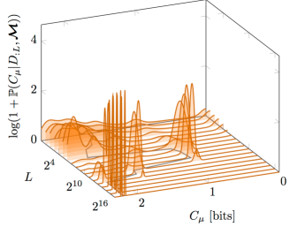
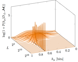
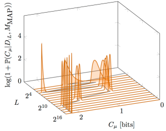
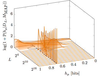
Figure S8: Simple Nonunifilar Source, $\beta=2$: Convergence of the posterior densities for $C_{\mu}$ (top) and $h_{\mu}$ (bottom) as a function of subsample length $L$ using the set of all topological $\epsilon$-machines with one- to five-states $\bm{\mathcal{M}}$ (left column) and the maximum a posteriori model $M_{\mbox{MAP}}$ (right column). In each panel, the black, dashed line indicates the true value and the gray, solid line shows the posterior mean.

Appendix E Number of Accepting Topologies for Processes

Appendix F Maximum a posteriori topologies

Figure S11 lists all MAP topologies encountered when inferring $\epsilon$-machine structure using data from the Even, Golden Mean, and SNS Processes. All processes had n1k2id3 (panel A) as the MAP topology for small $L$, reflecting a preference for small structures when limited data is available. The Golden Mean Process transitioned from n1k2id3 to n2k2id5 (panel B), the correct structure, at $L=64$, as documented in Table S2. In a similar manner, the Even Processes changed from n1k2id3 to n2k2id7 (panel C), the correct structure, at data size $L=32$, as shown in Table S4. The fact that these in-class $\epsilon$-machine structures quickly converge on the correct topology is perhaps expected. Predicting the sample size at which this occurs, however, is not obvious.

The Simple Nonunifilar Source has a more complicated series of MAP topologies, starting with the simple n1k2id3 and progressing through n2k2id5 (panel B), to n4k2id3334 (panel D) and, finally, to n5k2id22979 (panel E) at data size $2^{17}$. Of course, this out-of-class data source cannot be exactly captured by the set of finite-state unifilar $\epsilon$-machines considered here. Nonetheless, we expect the size of the inferred model to increase if more data from the SNS were employed and a larger numbers of states were allowed. It is important to note that the MAP structure in this case has very low posterior probability. As discussed in the main text, the topology listed is one of five similar structures with nearly equal posterior probabilities.

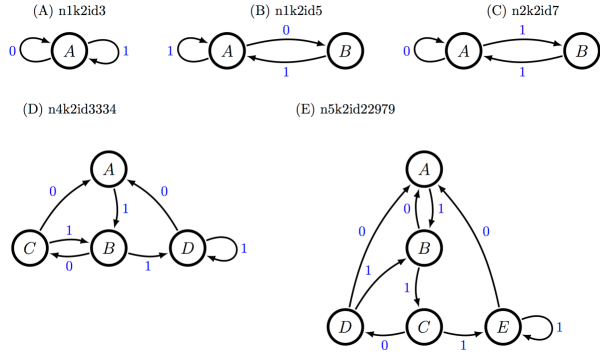
Figure S11: Maximum a posteriori topologies for the Golden Mean, Even, and SNS Process data series. Transitions are only listed with emitted output symbol. Transition probabilities are inferred from data for states that have more than one out-going transition. Transitions from states with only one out-going arc must have probability one, by definition of the topology. Consult Tables S2, S4, and S6 to see when these structures corresponded to the MAP topologies for the given data sources.

References

- [1] B.-J. Yoon. Hidden Markov models and their applications in biological sequence analysis. Curr. Genomics, 10:402–415, 2009.
- [2] L. Narlikar, N. Mehta, S. Galande, and M. Arjunwadkar. One size does not fit all: On how Markov model order dictates performance of genomic sequence analyses. Nucleic Acids Res., 2012.
- [3] R. L. Davidchack, Y.-C. Lai, E. M. Bollt, and M. Dhamala. Estimating generating partitions of chaotic systems by unstable periodic orbits. Phys. Rev. E, 61:1353–1356, 2000.
- [4] C. S. Daw, C. E A Finney, and E. R. Tracy. A review of symbolic analysis of experimental data. Rev. Sci. Instrum., 74:915–930, 2003.
- [5] M. B. Kennel and M. Buhl. Estimating good discrete partitions from observed data: Symbolic false nearest neighbors. Phys. Rev. Lett., 91:084102, 2003.
- [6] C. C. Strelioff and J. P. Crutchfield. Optimal instruments and models for noisy chaos. CHAOS, 17:043127, 2007.
- [7] R. P. N. Rao, N. Yadav, M. N. Vahia, H. Joglekar, R. Adhikari, and I. Mahadevan. A Markov model of the Indus script. Proc. Natl. Acad. Sci. USA, 106:13685–13690, 2009.
- [8] R. Lee, P. Jonathan, and P. Ziman. Pictish symbols revealed as a written language through application of Shannon entropy. Proc. Roy. Soc. A, 2010.
- [9] D. Kelly, M. Dillingham, A. Hudson, and K. Wiesner. A new method for inferring hidden Markov models from noisy time sequences. PLoS ONE, 7:e29703, 2012.
- [10] C.-B. Li, H. Yang, and T. Komatsuzaki. Multiscale complex network of protein conformational fluctuations in single-molecule time series. Proc. Natl. Acad. Sci. USA, 105:536–541, 2008.
- [11] P. Graben, J. D. Saddy, M. Schlesewsky, and J. Kurths. Symbolic dynamics of event-related brain potentials. Phys. Rev. E, 62:5518–5541, 2000.
- [12] R. Haslinger, K. L. Klinkner, and C. R. Shalizi. The computational structure of spike trains. Neural Comput, 22:121–157, 2009.
- [13] D. P. Varn, G. S. Canright, and J. P. Crutchfield. Inferring pattern and disorder in close-packed structures via -machine reconstruction theory: Structure and intrinsic computation in zinc sulphide. Acta. Cryst. Sec. B, 63(2):169–182, 2007.
- [14] D. P. Varn, G. S. Canright, and J. P. Crutchfield. -Machine spectral reconstruction theory: A direct method for inferring planar disorder and structure from X-ray diffraction studies. Acta. Cryst. Sec. A, 69(2):197–206, 2013.
- [15] J. P. Crutchfield. Between order and chaos. Nature Physics, 8(January):17–24, 2012.
- [16] J. P. Crutchfield and K. Young. Inferring statistical complexity. Phys. Rev. Let., 63:105–108, 1989.
- [17] D. P. Varn, G. S. Canright, and J. P. Crutchfield. Discovering planar disorder in close-packed structures from X-Ray diffraction: Beyond the fault model. Phys. Rev. B, 66(17):174110–3, 2002.
- [18] C. R. Shalizi, K. L. Shalizi, and J. P. Crutchfield. Pattern discovery in time series, Part I: Theory, algorithm, analysis, and convergence. 2002. Santa Fe Institute Working Paper 02-10-060; arXiv.org/abs/cs.LG/0210025.
- [19] C. R. Shalizi, K. L. Shalizi, and R. Haslinger. Quantifying self-organization with optimal predictors. Phys. Rev. Lett., 93:118701, 2004.
- [20] B. D. Johnson, J. P. Crutchfield, C. J. Ellison, and C. S. McTague. Enumerating finitary processes. 2012. SFI Working Paper 10-11-027; arxiv.org:1011.0036 [cs.FL].
- [21] E. Ott. Chaos in Dynamical Systems. Cambridge University Press, New York, 1993.
- [22] S. H. Strogatz. Nonlinear Dynamics and Chaos: with applications to physics, biology, chemistry, and engineering. Addison-Wesley, Reading, Massachusetts, 1994.
- [23] D. Lind and B. Marcus. An Introduction to Symbolic Dynamics and Coding. Cambridge University Press, New York, 1995.
- [24] A. B. Gelman, J. S. Carlin, H. S. Stern, and D. B. Rubin. Bayesian Data Analysis. Chapman & Hall, CRC, 1995.
- [25] C. R. Shalizi and J. P. Crutchfield. Computational mechanics: Pattern and prediction, structure and simplicity. J. Stat. Phys., 104:817–879, 2001.
- [26] N. Travers and J. P. Crutchfield. Exact synchronization for finite-state sources. J. Stat. Phys., 145(5):1181–1201, 2011.
- [27] N. Travers and J. P. Crutchfield. Asymptotic synchronization for finite-state sources. J. Stat. Phys., 145(5):1202–1223, 2011.
- [28] N. Travers and J. P. Crutchfield. Equivalence of history and generator -machines. 2011. SFI Working Paper 11-11-051; arxiv.org:1111.4500 [math.PR].
- [29] C. C. Strelioff, J. P. Crutchfield, and A. W. Hübler. Inferring Markov chains: Bayesian estimation, model comparison, entropy rate, and out-of-class modeling. Phys. Rev. E, 76:011106, 2007.
- [30] C. J. Ellison, J. R. Mahoney, and J. P. Crutchfield. Prediction, retrodiction, and the amount of information stored in the present. J. Stat. Phys., 136(6):1005–1034, 2009.
- [31] C. J. Ellison and J. P. Crutchfield. States of states of uncertainty. page arxiv.org: 13XX.XXXX, in preparation.
- [32] L. Rabiner. A tutorial on hidden Markov models and selected applications in speech recognition. Proc. IEEE, 77:257–286, 1989.
- [33] S. S. Wilks. Mathematical Statistics. John Wiley & Sons, Inc., New York, NY, 1962.
- [34] D. H. Wolpert and D. R. Wolf. Estimating functions of probability distributions from a finite set of samples. Phys. Rev. E, 52:6841–6854, 1995.
- [35] L. Yuan and H. K. Kesavan. Bayesian estimation of Shannon entropy. Commun. Stat. Theory Methods, 26:139–148, 1997.
- [36] J. P. Crutchfield. The calculi of emergence: Computation, dynamics, and induction. Physica D, 75:11–54, 1994.
- [37] K. J. Lang, B. A. Pearlmutter, and R. A. Price. Results of the Abbadingo One DFA learning competition and a new evidence-driven state merging algorithm. In V. Honavar and G. Slutzki, editors, Grammatical Inference, volume 1433 of Lect. Notes Comp. Sci., pages 1–12. Springer Berlin Heidelberg, 1998.
- [38] C. de la Higuera. A bibliographical study of grammatical inference. Patt. Recog., 38:1332–1348, 2005.
Supplementary Material