Properties of M31. III: Candidate Beat Cepheids from PS1 PAndromeda Data and Their Implication on Metallicity Gradient

Abstract

We present a sample of M31 beat Cepheids from the Pan-STARRS 1 PAndromeda campaign. By analyzing three years of PAndromeda data, we identify seventeen beat Cepheids, spreading from a galactocentric distance of 10 to 16 kpc. Since the relation between fundamental mode period and the ratio of fundamental to the first overtone period puts a tight constraint on metallicity we are able to derive the metallicity at the position of the beat Cepheids using the relations from the model of Buchler (2008). Our metallicity estimates show sub-solar values within 15 kpc, similar to the metallicities from HII regions (Zurita & Bresolin, 2012). We then use the metallicity estimates to calculate the metallicity gradient of the M31 disk, which we find to be closer to the metallicity gradient derived from planetary nebula (Kwitter et al., 2012) than the metallicity gradient from HII regions (Zurita & Bresolin, 2012).

1 Introduction

Beat Cepheids are pulsating simultaneously in two radial modes. Studies of beat Cepheids can be dated back to Oosterhoff (1957a, b), where he introduced a beat period to explain the large scattered photometric measurements of U TrA and TU Cas in the Milky Way. Several attempts to search for Galactic beat Cepheids have been conducted (see e.g. Pike & Andrews, 1979; Henden, 1979, 1980), however, only 20 Galactic beat Cepheids are documented to-date (see e.g. McMaster Cepheid Data Archive , where 651 Type I Cepheids and 209 Type II Cepheids are listed as well). The first larger samples of beat Cepheids have been identified in microlensing survey data. For example, the MACHO project has discovered 45 beat Cepheids in the Large Magellanic Cloud, where 30 are pulsating in the fundamental mode and first overtone, while 15 are pulsating in the first and second overtone (Alcock et al., 1995). The OGLE team found 93 beat Cepheids in the Small Magellan Clouds (Udalski et al., 1999) and 76 beat Cepheids in the Large Magellanic Clouds (Soszynski et al., 2000). A recent study from the EROS group has increased the number of known beat Cepheids in the Magellanic clouds to over 200 (Marquette et al., 2009). The OGLE-III survey has found the largest number of beat Cepheids so far: 271 objects in the LMC (Soszynski et al., 2008) and 277 in the SMC (Soszynski et al., 2010). These numbers will be even larger during the currently conducted OGLE-IV phase.

Beat Cepheids pulsating in the fundamental mode and first overtone can be used as a tracer of the metallicity content within a galaxy. This is because from modelling, there exists only a sub-region in the parameter spaces of mass, luminosity, temperature, and metallicity where both the fundamental mode and first overtone are linearly unstable (see e.g. Kolláth et al., 2002). Beaulieu et al. (2006) have thus made use of the beat Cepheids found in the CFHT M33 survey (Hartman et al., 2006) and derived the metallicity gradient of M33 to be -0.16 dex/kpc. Their metallicity gradient supports the HII region result from Garnett et al. (1997) but disagrees with the much shallower gradient from Crockett et al. (2006), who also used HII region to derive the metallicity. It is important to note that both results from Garnett et al. (1997) and Crockett et al. (2006) are derived from HII regions, yet are inconsistent with each other.

In this study we present a sample of beat Cepheids identified from the PS1 PAndromeda project. We derive the metallicity gradient of M31 and compare our results with previous studies of HII regions and planetary nebulae. Our paper is composed as follows. In section 2 we demonstrate our method to search for beat Cepehids. We elucidate the approach to derive metallicity in section 3. The metallicity gradient of M31 from our sample, as well as a comparison with previous HII region and planetary nebulae method is presented in section 4, followed by a conclusion and outlook in section 5.

2 Beat Cepheid Identification

We use the optical data taken by the PAndromeda project to search for beat Cepheids. PAndromeda monitors the Andromeda galaxy with the 1.8m PS1 telescope with a $\sim$ 7 deg² field-of-view (see Kaiser et al., 2010; Hodapp et al., 2004; Tonry & Onaka, 2009, for a detailed description of the PS1 system, optical design, and the imager). Observations are taken in $r_{\rm P1}$ and $i_{\rm P1}$ on daily basis during July to December in order to search for microlensing events and variables. Several exposures in $g_{\rm P1}$, $z_{\rm P1}$, and $y_{\rm P1}$ are also taken as complementary information for studies on the stellar content.

The data reduction is based on the MDia tool (Koppenhoefer et al., 2013) and is explained in Lee et al. (2012) in detail. We outline our data reduction steps as follows. The raw data are detrended by the image processing pipeline (IPP, Magnier, 2006) and warped to a sky-based image plane (so-called skycells). The images at the skycell stage are further analyzed by our sophisticated imaging subtraction pipeline mupipe (Gössl & Riffeser, 2002) based on the idea of image differencing analysis advocated by Alard & Lupton (1998). This includes the creation of deep reference images from best seeing data, stacking of observations within one visit to have better signal to noise ratio (hereafter “visit stacks”), subtraction of visit stacks from the reference images to search for variability, and creating light-curves from the subtracted images.

We have shown in Kodric et al. (2013) how to obtain Cepheid light-curves in the PAndromeda data. The major difference is that the data-set used in this work contains three years of PAndromeda, instead of one year and a few days from the second year data used in Kodric et al. (2013). The sky tessellation is also different, in order to have the central region of M31 in the center of a skycell (skycell 045), instead of at the corner of adjacent skycells (skycell number 065, 066, 077, and 078) as in Kodric et al. (2013); the skycells are larger and overlap in the new tessellation. The new tessellation is drawn in Fig. 1. We have extended the analysis to 47 skycells, twice as many as the number of skycells used in Kodric et al. (2013). The skycells we used are 012-017, 022-028, 032-038, 042-048, 052-058, 062-068, 072-077, which cover the whole of M31. The search of Cepheids is conducted in both $r_{\rm P1}$ and $i_{\rm P1}$, where we start from the resolved sources in the $r_{\rm P1}$ reference images, and require variability in both $r_{\rm P1}$ and $i_{\rm P1}$ filters. In addition one could search for variables also in the pixel-based light-curves. This approach would add light-curves for fainter variable sources (among them potentially lower period Cepheids) which we do not aim to study in this work.

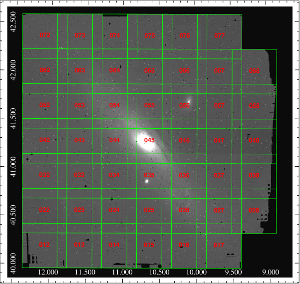
Figure 1: Illustration of our new tessellation. The background image is a mosaic of reference images from all skycells analyzed in this work.

We use the SigSpec package (Reegen, 2007) to determine the period of all variables. For a given light-curve, we iterate the period search five times both in $r_{\rm P1}$ and $i_{\rm P1}$ to search for multiple periods. In each iteration, SigSpec computes the significance spectrum and determines the most significant period. It then fits a multi-sine function based on this period, subtracts the best-fitted multi-sine curve to the input light-curve, and performs another iteration of period search based on this pre-whitened light-curve.

For the beat Cepheids, we look for sources that are showing only two significant periods (i.e. where SigSpec does not find a period after the second iteration). We also require that both periods are found in $r_{\rm P1}$ and $i_{\rm P1}$ light-curves and are consistent within ten percent. We adopt the period derived from $r_{\rm P1}$ as final period, due to the better sampling and the higher amplitude than the $i_{\rm P1}$-band light-curves. This leads to a sample of seventeen beat Cepheids. Their locations, periods in fundamental mode (P₀) and first overtone (P₁) , and light-curves are shown in Fig. 2, Fig. 3, and Table 2. In the next section, we present their metallicities derived from the period and the period ratio. Given the periods and metallicities, we are also able to obtain an estimate of their ages.

Name	RA	Dec	P${}_{0}^{r_{\rm P1}}$	P${}_{1}^{r_{\rm P1}}$	P${}_{1}^{r_{\rm P1}}$/P${}_{0}^{r_{\rm P1}}$	P${}_{0}^{i_{\rm P1}}$	P${}_{1}^{i_{\rm P1}}$	P${}_{1}^{i_{\rm P1}}$/P${}_{0}^{i_{\rm P1}}$
	(J2000)	(J2000)	[days]	[days]		[days]	[days]
PSO J010.0031+40.6271	10.00313	40.62716	5.08121$\pm$0.00131	3.57641$\pm$0.00049	0.703850	5.08163$\pm$0.00790	3.57673$\pm$0.00161	0.703855
PSO J010.0289+40.6434	10.02891	40.64346	4.42890$\pm$0.00084	3.11390$\pm$0.00071	0.703087	4.42311$\pm$0.00269	3.11339$\pm$0.00099	0.703892
PSO J010.0908+40.8632	10.09082	40.86323	3.82737$\pm$0.00050	2.69071$\pm$0.00028	0.703018	3.82750$\pm$0.00103	2.69091$\pm$0.01056	0.703046
PSO J010.1097+41.1233	10.10973	41.12339	3.88787$\pm$0.00057	2.76180$\pm$0.00049	0.710363	3.88655$\pm$0.00129	2.76147$\pm$0.00076	0.710520
PSO J010.1601+41.0591	10.16016	41.05914	4.81211$\pm$0.00068	3.37280$\pm$0.00057	0.700898	4.81242$\pm$0.00120	3.37283$\pm$0.00140	0.700859
PSO J010.2081+40.5311	10.20820	40.53114	3.73484$\pm$0.00059	2.66164$\pm$0.00085	0.712652	3.73517$\pm$0.00191	2.66181$\pm$0.01328	0.712634
PSO J010.3333+41.2202	10.33331	41.22027	3.96209$\pm$0.00066	2.82765$\pm$0.00021	0.713676	3.96449$\pm$0.00257	2.82771$\pm$0.00043	0.713259
PSO J010.3431+40.8255	10.34310	40.82556	8.68802$\pm$0.00299	6.02351$\pm$0.00240	0.693312	8.69612$\pm$0.00515	6.02638$\pm$0.00361	0.692996
PSO J010.5507+40.8208	10.55071	40.82087	4.68226$\pm$0.00140	3.28483$\pm$0.00052	0.701548	4.67941$\pm$0.00300	3.28542$\pm$0.00074	0.702101
PSO J010.6214+41.4763	10.62146	41.47634	5.86549$\pm$0.00125	4.08473$\pm$0.00099	0.696400	5.86891$\pm$0.00338	4.08356$\pm$0.02249	0.695795
PSO J010.8571+41.7272	10.85714	41.72723	4.12749$\pm$0.00071	2.93815$\pm$0.00049	0.711849	4.12611$\pm$0.00164	2.93745$\pm$0.00260	0.711918
PSO J011.2784+41.8935	11.27840	41.89359	4.77328$\pm$0.00088	3.37092$\pm$0.00056	0.706206	4.77551$\pm$0.02909	3.34082$\pm$0.01690	0.699573
PSO J011.3670+41.7533	11.36709	41.75335	8.26314$\pm$0.00167	5.78110$\pm$0.00110	0.699625	8.26723$\pm$0.00300	5.78289$\pm$0.00169	0.699495
PSO J011.3993+41.6778	11.39932	41.67789	4.81283$\pm$0.00192	3.39273$\pm$0.00053	0.704935	4.81013$\pm$0.00356	3.39258$\pm$0.00090	0.705299
PSO J011.4131+42.0052	11.41317	42.00529	3.66634$\pm$0.00081	2.60609$\pm$0.00043	0.710815	3.66630$\pm$0.00272	2.60564$\pm$0.00130	0.710700
PSO J011.4436+41.9044	11.44369	41.90446	2.37187$\pm$0.00066	1.69231$\pm$0.00032	0.713492	2.37164$\pm$0.00096	1.69201$\pm$0.00750	0.713435
PSO J011.4835+42.1621	11.48356	42.16218	6.09759$\pm$0.00176	4.25145$\pm$0.00131	0.697234	6.09709$\pm$0.00277	4.25231$\pm$0.00364	0.697433
Table 1: Location and periods of our beat Cepheid sample. We high-lighted the $r_{\rm P1}$-band columns in because these are the ones we adopt for the final analysis.

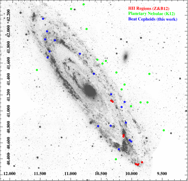
Figure 2: Spatial distribution of our sample (blue circle), HII regions in Zurita & Bresolin (2012), and planetary nebulae in Kwitter et al. (2012), over-plotted with GALEX NUV image (Gil de Paz et al., 2007).

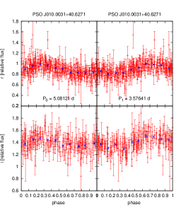
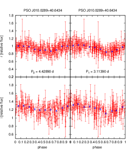
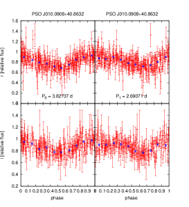
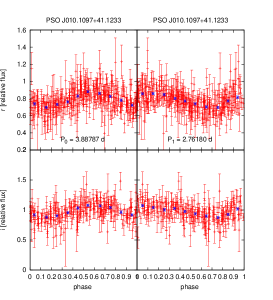
Figure 3: Light-curves of our sample. We fold the light-curves with the $r_{\rm P1}$-band period of fundamental mode P₀ (left-hand side) and first overtone P₁ (right-hand side). The red points are un-binned data, while the blue points are data binned with 0.1 phase interval.

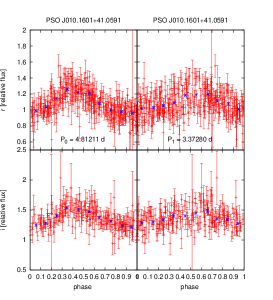
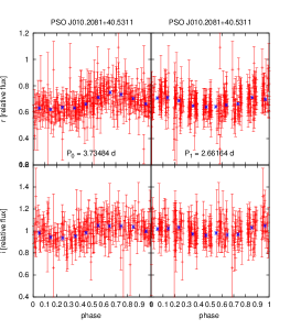
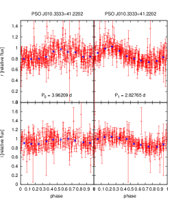
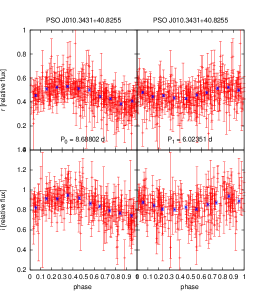
Figure 3: Light-curves of our sample - continued.

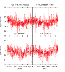
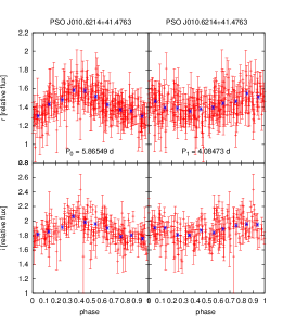
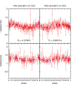
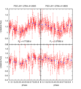
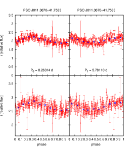
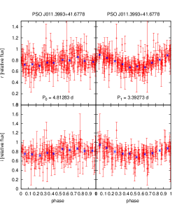
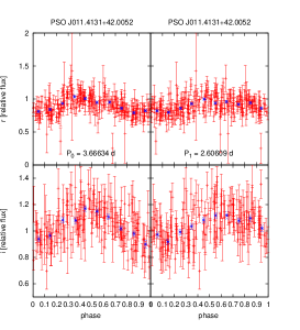
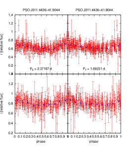
Figure 3: Light-curves of our sample - continued.

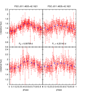
Figure 3: Light-curves of our sample - continued.

Figure 3: Light-curves of our sample - continued.

3 Metallicity Estimate

Given a uniquely measured period (P₀) and period ratio (P₁/P₀) of a beat Cepheid, the pulsation models only allow a sub-region in the parameter spaces of mass, luminosity, temperature, and metallicity for stable double mode pulsations. This enables us to narrow down the metallicity of the beat Cepheids (Beaulieu et al., 2006). As has been shown by Buchler (2008), one can derive the upper and lower metallicity limits simply by the location of a beat Cepheid on the log($P_{0}$) v.s. P₁/P₀ diagram (the so-called Petersen diagram, Petersen 1973). In the paper of (Buchler & Szabó, 2007; Buchler, 2008), they have shown that the metallicity estimates from this method fall in the generally accepted ballpark for Magellanic Clouds and M33. Fig. 4 shows our M31 sample on the Petersen diagram, as well as beat Cepheids from Milky Way, Large and Small Magellanic Clouds, and M33 with tracks of different metallicities taken from Buchler (2008). Our sample - similar to the beat Cepheids in the Milky Way - is on the metal rich side. On the other hand, the beat Cepheids in the Magellanic Clouds appear to be metal poor.

We interpolate the theoretical tracks by Buchler (2008) to derive the limits on the metallicity for our beat Cepheids. In Buchler (2008), two different solar mixtures are compared, one from Grevesse & Noels (1993), and the other from Asplund et al. (2005). In this work we use the metallicity tracks based on the solar mixture of Grevesse & Noels (1993), which agree better with the commonly used values. The metallicity is derived as follows. From the theoretical tracks by Buchler (2008), one can delimit the lower (Z_min, Fig. 4, left-hand side) and upper (Z_max, Fig. 4, right-hand side) boundaries of a given position in the Petersen diagram by interpolating between isometallictiy lines. We adopt the average of Z_min and Z_max as the metallicity estimate Z. The uncertainty is taken as $\frac{Z_{max}-Z_{min}}{2}$. For example, PSO J011.4436+41.9044 has log P₀ $\sim$ 0.38 and P₁/P₀ $\sim$ 0.7135; On Fig. 4, its lower boundary Z_min is bracketed by isometallicity lines Z = 0.009 and 0.010, while its upper boundary Z_max is between Z = 0.011 and 0.012, as also shown in the zoom-in for Petersen diagram in Fig. 5. By interpolation, we thus derive Z_min = 0.0098 and Z_max = 0.01152. The metallicity estimate is thus Z = $\frac{Z_{max}+Z_{min}}{2}$ = 0.01066 and the uncertainty is $\frac{Z_{max}-Z_{min}}{2}$ = 0.00086. The derived metallicity and its error for our sample are shown in Table 2. We also explore the impact on the metallicity estimates from errors in P₁/P₀ and present the results in the appendix. In Fig. 7, when calculating lower boundary Z_min, we use P₁/P₀ + (error of P₁/P₀) instead of P₁/P₀; and for upper boundary Z_max, we use P₁/P₀ - (error of P₁/P₀). The results are shown in Table 3 in the appendix, where the metallicity estimates Z remain the same, with or without taking into account of error of P₁/P₀. Only the uncertainty of the metallicity estimates changes very slightly.

The fact that the uncertainties in the metallicity become large when log($P_{0}$) $\sim$ 0.84 only allows us to determine the value of Z for fifteen out of seventeen beat Cepheids in our sample.

Once we have the period and metallicity, we can use the period-age relation from Table 4 of Bono et al. (2005):

$$\mathrm{log}(t)=\alpha+\beta\mathrm{log}(P)$$ (1)

to derive the age of our sample. Here we use P${}_{0}^{r_{\rm P1}}$ to calculate the age. However, one should bear in mind that this period-age relation is for fundamental mode, but not specially for beat Cepheids. We adopt ($\alpha$, $\beta$) = (8.49, -0.79) for Z $<$ 0.007 , (8.41, -0.78) for Z between 0.007 and 0.015, and (8.31, -0.67) for Z between 0.015 and 0.025. The ages of our beat Cepheids are all in the order of $\sim$ 100 Myr, showing that they are tracing a rather young stellar population. The age estimates can be found in Table. 2.

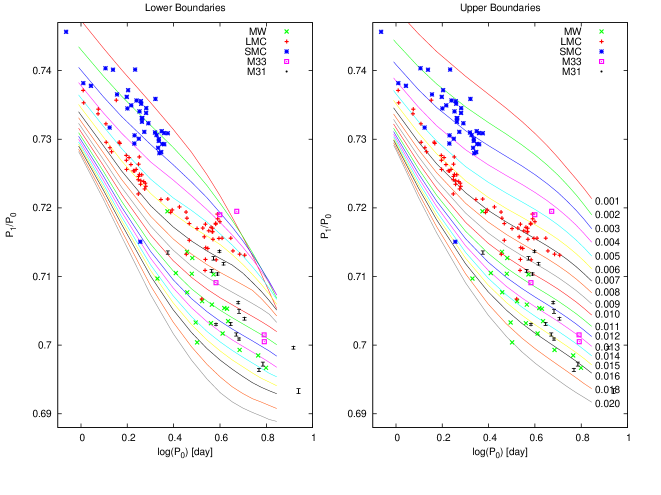
Figure 4: Petersen diagram of our sample (black symbols) and beat Cepheids of Milky Way (green crosses, from McMaster Cepheid Data Archive), Large and Small Magellanic Clouds (red and blue crosses, Marquette et al., 2009), and M33 (violet squares, Beaulieu et al., 2006). The period errors of our sample in terms of log(P₀) are too small to be seen in this figure. Track of different metallicities (Buchler, 2008) are shown as solid lines in different colors, where the corresponding metallicities are given in the right panel.

Figure 5: Zoom-in of the Petersen diagram on each candidate beat Cepheid. We show the adjacent theoretical isometallicity tracks and the interpolated Z values at the position of the beat Cepheids. The dashed and dash-dotted curves are isometallicity tracks from the theoretical work of Buchler (2008), which are the higher and lower isometallicity tracks adjacent to our measured log P₀ and P₁/P₀ values shown in black. The dotted isometallicity line is the interpolation that passes through our measured log P₀ and P₁/P₀ values. The estimated lower (Z_min, left subfigures) and upper (Z_max, right subfigures) metallicity limits are obtained from these interpolated values. We adopt the average of Z_min and Z_max as the metallicity estimate Z. The uncertainty is taken as $\frac{Z_{max}-Z_{min}}{2}$.

Figure 5: Zoom-in of the Petersen diagram - continued.

Figure 5: Zoom-in of the Petersen diagram - continued.

Name	log P0	Z	log($t$)	Distance	log(O/H)+12†
	[day]		[yr]	[kpc]
PSO J010.0031+40.6271	0.70597$\pm$0.00011	0.0116$\pm$0.0011	7.85935$\pm$0.00009	11.120	8.572$\pm$0.030
PSO J010.0289+40.6434	0.64630$\pm$0.00008	0.0129$\pm$0.0012	7.90589$\pm$0.00006	10.757	8.604$\pm$0.030
PSO J010.0908+40.8632	0.58290$\pm$0.00006	0.0140$\pm$0.0014	7.95534$\pm$0.00004	10.454	8.630$\pm$0.030
PSO J010.1097+41.1233	0.58971$\pm$0.00006	0.0091$\pm$0.0009	7.95002$\pm$0.00005	16.627	8.499$\pm$0.031
PSO J010.1601+41.0591	0.68234$\pm$0.00006	0.0139$\pm$0.0013	7.87778$\pm$0.00005	12.765	8.627$\pm$0.029
PSO J010.2081+40.5311	0.57227$\pm$0.00007	0.0081$\pm$0.0008	7.96363$\pm$0.00005	14.849	8.461$\pm$0.031
PSO J010.3333+41.2202	0.59792$\pm$0.00007	0.0073$\pm$0.0008	7.94362$\pm$0.00006	11.497	8.429$\pm$0.028
PSO J010.5507+40.8208	0.67046$\pm$0.00013	0.0136$\pm$0.0013	7.88704$\pm$0.00010	13.257	8.621$\pm$0.030
PSO J010.6214+41.4763	0.76830$\pm$0.00009	0.0158$\pm$0.0015	7.79524$\pm$0.00006	10.390	8.666$\pm$0.025
PSO J010.8571+41.7272	0.61569$\pm$0.00007	0.0081$\pm$0.0008	7.92976$\pm$0.00006	12.597	8.460$\pm$0.028
PSO J011.2784+41.8935	0.67882$\pm$0.00008	0.0105$\pm$0.0009	7.88052$\pm$0.00006	10.495	8.542$\pm$0.028
PSO J011.3993+41.6778	0.68240$\pm$0.00017	0.0112$\pm$0.0010	7.87773$\pm$0.00014	13.731	8.561$\pm$0.029
PSO J011.4131+42.0052	0.56423$\pm$0.00010	0.0092$\pm$0.0009	7.96990$\pm$0.00007	12.386	8.501$\pm$0.032
PSO J011.4436+41.9044	0.37509$\pm$0.00012	0.0107$\pm$0.0009	8.11743$\pm$0.00009	11.941	8.547$\pm$0.029
PSO J011.4835+42.1621	0.78516$\pm$0.00013	0.0149$\pm$0.0013	7.79758$\pm$0.00010	15.221	8.648$\pm$0.028

Table 2: Beat Cepheid properties; † See section 4 for a detailed explanation.

4 Metallicity gradient

To derive the metallicity gradient, we first de-project the coordinates of the beat Cepheids to galactocentric distances using the transformation of Haud (1981). We assume that the center of M31 is located at RA=00h42’44”.52 (J2000) and Dec=+41d16’08”.69 (J2000), with a position angle of 37d42’54”. We also assume an inclination angle of 12.5 degrees (Simien et al., 1978) and a distance of 770 kpc (Freedman & Madore, 1990).

To compare with previous results from HII region studies (Zurita & Bresolin, 2012; Sanders et al., 2012), which are shown in log(O/H), we first convert our Z values to [O/H] by using a Z_⊙ value of 0.017 and [O/H] = [Fe/H]/1.417 from Maciel et al. (2003). We then use log(O/H)_⊙ + 12 = 8.69 (Asplund et al., 2009) to calculate the values of log(O/H) + 12 for our sample, and compare them with previous results from the HII regions and planetary nebulae observations of M31 shown in Fig. 6.

There are several ways to extract the chemical abundance from spectroscopic observations of HII regions. For example, Zurita & Bresolin (2012) have determined the electron temperature of the gas from HII regions and derive the chemical abundance accordingly (so-called direct-$T_{e}$ method). On the other hand, one can use the flux ratio between strong lines to infer the chemical abundance of certain elements. For example, Sanders et al. (2012) have used the flux ratio between [N II] and H_α proposed by Nagao et al. (2006) to obtain the log(O/H) values from HII regions. In Fig. 2 and Fig. 6 we only show the eight HII region samples from Zurita & Bresolin (2012), because they are the only ones who derive $T_{e}$ and [O/H] values from the faint [O III] line directly. In Sanders et al. (2012), they have hundreds of HII region measurements, but their [O/H] value varies depending on which strong-lines are used. Our beat Cepheid result is closer to the metallicities from the direct method of Zurita & Bresolin (2012) than the strong-line mentioned. Our errors are much smaller than those for traditional metallicity measurement methods. As a consequence, the difference of our metallicity values to that of Zurita & Bresolin (2012) is significant.

In addition to the HII regions, chemical abundance can be derived from the planetary nebulae as well. We also compare our result to the metallicities from Kwitter et al. (2012) in Fig. 6. Contrary to the metallicities from planetary nebulae, our result shows sub-solar log(O/H) value within 15 kpc, similar to the result from HII regions. The mean log(O/H)+12 value from our sample is 8.56, while observations from planetary nebulae give a higher value (8.64). Our sample has a gradient of -0.008$\pm$0.004 dex/kpc, close to the value of -0.011$\pm$0.004 dex/kpc from planetary nebulae (Kwitter et al., 2012). Our result shows scatter around the linear gradient, which could originate from the intrinsic variation of in situ metallicity.

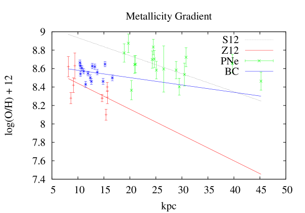
Figure 6: Metallicity as a function of de-projected distance to the center of M31. The blue crosses are derived from our sample (see section 4 for a detailed description). The black line is from Sanders et al. (2012), where they use the N2 diagnosis (strong line method) to obtain the log(O/H) values from HII regions. The red line and red data points (see our Fig. 2 for their positions) are from Zurita & Bresolin (2012). They determine the electron temperature of the gas from HII regions and derive the chemical abundance accordingly (direct method). The green points mark chemical abundances derived from planetary nebulae by Kwitter et al. (2012). Since planetary nebulae and beat Cepheids are tracing different stellar population, we expect different metallicity estimates from these two methods. Our result is closer to the results obtained with the direct method from HII region than to results obtained with the strong line method (grey dashed line). Also, our metallicities are significantly differ from the metallicities derived for planetary nebulae in the outer M31 disk.

The detailed properties of our sample, including the metallicity, galactocentric distance, and age are shown in Table 2.

5 Conclusion and Outlook

We present a sample of the beat Cepheids based on the PAndromeda data. We use the P₁/P₀ to P₀ relations from pulsation models of Buchler (2008) to estimate the Cepheid metallicities. We de-project the location of beat Cepheids, and derive the metallicity gradient of M31. Our result is closer to the results from the planetary nebulae of Kwitter et al. (2012).

In this work we only concentrate on searching beat Cepheids from a sample of resolved sources. In a future work we will also conduct searches for variables from pixel-based light-curves. In this case we could find fainter variables.

Because the beat Cepheids are pulsating at relative short periods, they are intrinsically very faint, and with a 2-m class telescope like PS1 it is difficult to find a large sample at the distance of M31. To increase the number of beat Cepheids in M31, it requires deeper surveys. Our understanding of beat Cepheid content in M31 can be improved with the CFHT POMME survey (Fliri & Valls-Gabaud, 2012) and the up-coming LSST project (Ivezic et al., 2008).

6 Appendix

In this section we explore the impact on the metallicity estimates from errors in P₁/P₀ and present the results. In Fig. 7, when calculating lower boundary Z_min, we use P₁/P₀ + (error of P₁/P₀) instead of P₁/P₀; and for upper boundary Z_max, we use P₁/P₀ - (error of P₁/P₀). The results are shown in Table 3, where the metallicity estimates Z remain the same, with or without taking into account of error of P₁/P₀. Only the uncertainty of the metallicity estimates changes very slightly.

Name	Z	Z
	without $\frac{P_{1}}{P_{0}}$-err	with $\frac{P_{1}}{P_{0}}$-err
J010.0031+40.6271	0.0116$\pm$0.0011	0.0116$\pm$0.0012
J010.0289+40.6434	0.0129$\pm$0.0012	0.0129$\pm$0.0014
J010.0908+40.8632	0.0140$\pm$0.0014	0.0140$\pm$0.0014
J010.1097+41.1233	0.0091$\pm$0.0009	0.0091$\pm$0.0010
J010.1601+41.0591	0.0139$\pm$0.0013	0.0139$\pm$0.0014
J010.2081+40.5311	0.0081$\pm$0.0008	0.0081$\pm$0.0010
J010.3333+41.2202	0.0073$\pm$0.0008	0.0073$\pm$0.0008
J010.5507+40.8208	0.0136$\pm$0.0013	0.0136$\pm$0.0015
J010.6214+41.4763	0.0158$\pm$0.0015	0.0158$\pm$0.0016
J010.8571+41.7272	0.0081$\pm$0.0008	0.0081$\pm$0.0009
J011.2784+41.8935	0.0105$\pm$0.0009	0.0105$\pm$0.0011
J011.3993+41.6778	0.0112$\pm$0.0010	0.0112$\pm$0.0012
J011.4131+42.0052	0.0092$\pm$0.0009	0.0092$\pm$0.0010
J011.4436+41.9044	0.0107$\pm$0.0009	0.0107$\pm$0.0010
J011.4835+42.1621	0.0149$\pm$0.0013	0.0149$\pm$0.0015

Table 3: Z of beat Cepheid properties; derived with and without taking into account errors in P₁/P₀.

Figure 7: Zoom-in of the Petersen diagram on each candidate beat Cepheid. We show the adjacent theoretical isometallicity tracks and the interpolated Z values at the position of the beat Cepheids. The dashed and dash-dotted curves are isometallicity tracks from the theoretical work of Buchler (2008), which are the higher and lower isometallicity tracks adjacent to our measured log P₀ and P₁/P₀ values shown in black. The dotted isometallicity line is the interpolation that passes through our measured log P₀ and P₁/P₀ values. The estimated lower (Z_min, left subfigures) and upper (Z_max, right subfigures) metallicity limits are obtained from these interpolated values.

Figure 7: Zoom-in of the Petersen diagram - continued.

Figure 7: Zoom-in of the Petersen diagram - continued.

References

- Alard & Lupton (1998) Alard, C., & Lupton, R. H. 1998, ApJ, 503, 325
- Alcock et al. (1995) Alcock, C., Allsman, R. A., Axelrod, T. S., et al. 1995, AJ, 109, 1653
- Asplund et al. (2005) Asplund, M., Grevesse, N., & Sauval, A. J. 2005, Cosmic Abundances as Records of Stellar Evolution and Nucleosynthesis, 336, 25
- Asplund et al. (2009) Asplund, M., Grevesse, N., Sauval, A. J., & Scott, P. 2009, ARA&A, 47, 481
- Beaulieu et al. (2006) Beaulieu, J.-P., Buchler, J. R., Marquette, J.-B., Hartman, J. D., & Schwarzenberg-Czerny, A. 2006, ApJ, 653, L101
- Bono et al. (2005) Bono, G., Marconi, M., Cassisi, S., et al. 2005, ApJ, 621, 966
- Buchler & Szabó (2007) Buchler, J. R., & Szabó, R. 2007, ApJ, 660, 723
- Buchler (2008) Buchler, J. R. 2008, ApJ, 680, 1412
- Crockett et al. (2006) Crockett, N. R., Garnett, D. R., Massey, P., & Jacoby, G. 2006, ApJ, 637, 741
- Fliri & Valls-Gabaud (2012) Fliri, J., & Valls-Gabaud, D. 2012, Ap&SS, 341, 57
- Freedman & Madore (1990) Freedman, W. L., & Madore, B. F. 1990, ApJ, 365, 186
- Garnett et al. (1997) Garnett, D. R., Shields, G. A., Skillman, E. D., Sagan, S. P., & Dufour, R. J. 1997, ApJ, 489, 63
- Gil de Paz et al. (2007) Gil de Paz, A., Boissier, S., Madore, B. F., et al. 2007, ApJS, 173, 185
- Gössl & Riffeser (2002) Gössl, C. A., & Riffeser, A. 2002, A&A, 381, 1095
- Grevesse & Noels (1993) Grevesse, N., & Noels, A. 1993, Origin and Evolution of the Elements, 15
- Hartman et al. (2006) Hartman, J. D., Bersier, D., Stanek, K. Z., et al. 2006, MNRAS, 371, 1405
- Haud (1981) Haud, U. 1981, Ap&SS, 76, 477
- Henden (1980) Henden, A. A. 1980, MNRAS, 192, 621
- Henden (1979) Henden, A. A. 1979, MNRAS, 189, 149
- Hodapp et al. (2004) Hodapp, K. W., Siegmund, W. A., Kaiser, N., et al. 2004, Proc. SPIE, 5489, 667
- Ivezic et al. (2008) Ivezic, Z., Tyson, J. A., Acosta, E., et al. 2008, arXiv:0805.2366
- Kaiser et al. (2010) Kaiser, N., Burgett, W., Chambers, K., et al. 2010, Proc. SPIE, 7733,
- Kodric et al. (2013) Kodric, M., Riffeser, A., Hopp, U., et al. 2013, AJ, 145, 106
- Kolláth et al. (2002) Kolláth, Z., Buchler, J. R., Szabó, R., & Csubry, Z. 2002, A&A, 385, 932
- Koppenhoefer et al. (2013) Koppenhoefer, J., Saglia, R. P., & Riffeser, A. 2013, Experimental Astronomy, 35, 329
- Kwitter et al. (2012) Kwitter, K. B., Lehman, E. M. M., Balick, B., & Henry, R. B. C. 2012, ApJ, 753, 12
- Lee et al. (2012) Lee, C.-H., Riffeser, A., Koppenhoefer, J., et al. 2012, AJ, 143, 89
- Maciel et al. (2003) Maciel, W. J., Costa, R. D. D., & Uchida, M. M. M. 2003, A&A, 397, 667
- Magnier (2006) Magnier, E. 2006, The Advanced Maui Optical and Space Surveillance Technologies Conference,
- Marquette et al. (2009) Marquette, J. B., Beaulieu, J. P., Buchler, J. R., et al. 2009, A&A, 495, 249
- Nagao et al. (2006) Nagao, T., Maiolino, R., & Marconi, A. 2006, A&A, 459, 85
- Oosterhoff (1957a) Oosterhoff, P. T. 1957, Bull. Astron. Inst. Netherlands, 13, 317
- Oosterhoff (1957b) Oosterhoff, P. T. 1957, Bull. Astron. Inst. Netherlands, 13, 320
- Petersen (1973) Petersen, J. O. 1973, A&A, 27, 89
- Pike & Andrews (1979) Pike, C. D., & Andrews, P. J. 1979, MNRAS, 187, 261
- Reegen (2007) Reegen, P. 2007, A&A, 467, 1353
- Sanders et al. (2012) Sanders, N. E., Caldwell, N., McDowell, J., & Harding, P. 2012, ApJ, 758, 133
- Simien et al. (1978) Simien, F., Pellet, A., Monnet, G., et al. 1978, A&A, 67, 73
- Soszynski et al. (2000) Soszynski, I., Udalski, A., Szymanski, M., et al. 2000, Acta Astron., 50, 451
- Soszynski et al. (2008) Soszynski, I., Poleski, R., Udalski, A., et al. 2008, Acta Astron., 58, 163
- Soszynski et al. (2010) Soszynski, I., Poleski, R., Udalski, A., et al. 2010, Acta Astron., 60, 17
- Tonry & Onaka (2009) Tonry, J., & Onaka, P. 2009, Advanced Maui Optical and Space Surveillance Technologies Conference,
- Udalski et al. (1999) Udalski, A., Soszynski, I., Szymanski, M., et al. 1999, Acta Astron., 49, 1
- Zurita & Bresolin (2012) Zurita, A., & Bresolin, F. 2012, MNRAS, 427, 1463