On the influence of physical galaxy properties on Ly$\alpha$ escape in star-forming galaxies

Abstract

Context. Among the different observational techniques used to select high-redshift galaxies, the hydrogen recombination line Lyman-alpha (Ly$\alpha$) is of particular interest as it gives access to the measurement of cosmological quantities such as the star formation rate of distant galaxy populations. However, the interpretation of this line and the calibration of such observables is still subject to serious uncertainties.

Aims. In this context, it important to understand the mechanisms responsible for the attenuation of Ly$\alpha$ emission, and under what conditions the Ly$\alpha$ emission line can be used as a reliable star formation diagnostic tool

Methods. We use a sample of 24 Ly$\alpha$ emitters at $z\sim 0.3$ with an optical spectroscopic follow-up to calculate the Ly$\alpha$ escape fraction and its dependency upon different physical properties. We also examine the reliability of Ly$\alpha$ as a star formation rate indicator. We combine these observations with a compilation of Ly$\alpha$ emitters selected at $z=0-0.3$ from the literature to assemble a larger sample.

Results. We confirm that the Ly$\alpha$ escape fraction depends clearly on the dust extinction following the relation $f_{esc}$(Ly$\alpha$)$=C_{Ly\alpha}\times 10^{-0.4\leavevmode\nobreak\ E(B-V)\leavevmode\nobreak\ k_{Ly\alpha}}$ where $k_{Ly\alpha}\sim 6.67$ and C${}_{Ly\alpha}=0.22$. However, the correlation does not follow the expected curve for a simple dust attenuation. A higher attenuation can be attributed to a scattering process, while $f_{esc}$(Ly$\alpha$) values that are clearly above the continuum extinction curve can be the result of various mechanisms that can lead to an enhancement of the Ly$\alpha$ output. We also observe that the strength of Ly$\alpha$ and the escape fraction appear unrelated to the galaxy metallicity. Regarding the reliability of Ly$\alpha$ as a star formation rate (SFR) indicator, we show that the deviation of SFR(Ly$\alpha$) from the true SFR (as traced by the UV continuum) is a function of the observed SFR(UV), which can be seen as the decrease of $f_{esc}$(Ly$\alpha$) with increasing UV luminosity. Moreover, we observe redshift-dependence of this relationship revealing the underlying evolution of $f_{esc}$(Ly$\alpha$) with redshift.

1 Introduction

The study of galaxy formation and evolution is strongly related to the observational techniques used to detect galaxy populations at different epochs. In particular, the detection of the Ly$\alpha$ emission line in very distant galaxies has triggered many cosmological applications. The Ly$\alpha$ line is predicted to be the dominant spectral signature in young galaxies (Charlot & Fall 1993; Schaerer 2003), and combined to its rest-frame wavelength in the UV, one obtains a very efficient tool to detect galaxies at $2<z<7$ in the optical window from ground-based telescopes. Therefore, this potential has often been used to assemble large samples of star-forming galaxies at high redshift (e.g. Gronwall et al. 2007; Nilsson et al. 2009; Ouchi et al. 2010; Hayes et al. 2010; Cassata et al. 2011; Kashikawa et al. 2011). Ly$\alpha$-based samples additionally offer the opportunity of constraining the stage of cosmic reionization using the expected sharp drop in their number density as the ionization state of the intergalactic medium (IGM) changes (eg. Malhotra & Rhoads 2006), or the shape of the Ly$\alpha$ line profile itself (Kashikawa et al. 2006; Dijkstra & Wyithe 2010).

The interpretation of the Ly$\alpha$-based observations hinges however on a complete understanding of the redshift-evolution of the intrinsic properties of galaxies, the physical properties responsible for Ly$\alpha$ emission, and how the Ly$\alpha$ emitters (LAEs) are related to other galaxy populations. Given the different selection methods, it is still unclear how the LAE population is connected to the Lyman-Break Galaxies (LBGs) selected upon their rest-frame UV continuum. The possible overlap between these galaxy populations has been questioned in many studies recently but no definitive answer has emerged yet. Specifically, only a fraction of LBGs (Shapley et al. 2003) and H$\alpha$ emitting galaxies (Hayes et al. 2010) show Ly$\alpha$ in emission , and LBGs appear to be more massive, dustier and older (e.g. Gawiser et al. 2006; Erb et al. 2006). A reasonable scenario attributes these observed differences to the radiative transport of Ly$\alpha$ photons in the ISM (Schaerer & Verhamme 2008; Verhamme et al. 2008; Pentericci et al. 2010). Most observed trends of Ly$\alpha$ would be driven by variations of $N$(Hi) and the accompanying variation of the dust content that will dramatically enhance the suppression of the Ly$\alpha$ line as shown in Atek et al. (2009b). However, Kornei et al. (2010) found that Ly$\alpha$ emission is stronger in older and less dusty galaxies, and Finkelstein et al. (2009b) found that Ly$\alpha$ emission is stronger in massive and old galaxies. Although these results are still model-dependent, as they rely on SED fitting to infer the stellar population properties, they are apparently not compatible with the radiative transfer scenario.

We have been until recently in the curious situation, where we studied thousands of LAEs at redshift $z\sim 2$ and higher, whereas only a handful of Ly$\alpha$ galaxies is available in the nearby universe without any statistical bearing, since such studies are hampered by the difficulty to obtain UV observations. In the past few years, the situation has changed significantly with the advent of the Galaxy Evolution Explorer (GALEX, Martin 2005) whose UV grism capabilities enabled the study of a large sample of UV-selected galaxies at $z\ \lower 2.15277pt\hbox{$\buildrel<\over{\sim}$}\leavevmode\nobreak\ 1$ (Deharveng et al. 2008; Atek et al. 2009a; Finkelstein et al. 2009a; Scarlata et al. 2009; Cowie et al. 2010). The study of low-redshift LAEs offers the advantage of a much higher flux and the possibility to obtain critical complementary informations at longer wavelengths in subsequent optical follow-up observations. We obtained in Atek et al. (2009a) optical spectroscopy for a subsample of LAEs detected by GALEX at a redshift of $z\sim 0.3$. Using optical emission lines, we were able for the first time to empirically measure the Ly$\alpha$ escape fraction $f_{esc}$(Ly$\alpha$) in a sample of LAEs and found a clear anti-corellation with the dust extinction. Other studies derived the same quantity at different redshifts and find in general the same trend (Scarlata et al. 2009; Kornei et al. 2010; Hayes et al. 2010). Nevertheless, all these results show a large scatter around the $f_{esc}$(Ly$\alpha$)-dust relationship, which is presumably the result of a number of other physical parameters that may affect the Ly$\alpha$ escape fraction.

The next generation of telescopes James Webb Space Telescope JWST and Extremely Large Telescopes (ELTs) will heavily depend on Ly$\alpha$ as a detection and star-formation diagnostic tool in distant galaxies. Therefore, it is crucial that we understand how to retrieve the intrinsic Ly$\alpha$ emission from the observed quantity in order to properly derive the cosmological quantities. Consequently, the Ly$\alpha$ escape fraction represents a key-parameter for the interpretation of current and future Ly$\alpha$ based surveys. Using our sample of $z\sim 0.3$ Ly$\alpha$ galaxies, we discuss in the present work the dependence of the Ly$\alpha$ escape fraction on the physical properties of the host galaxy. In Section 2, we present our spectroscopic follow-up of GALEX-detected LAEs and the sample of local galaxies included in the study. We expose in Section 3 our emission-line measurements and the procedure we followed to derive the physical properties of our galaxies, i.e the metallicity and extinction estimates and the AGN/starburst classification. In Section 4, we discuss the correlation of Ly$\alpha$ with various parameters, while section 5 is devoted to the regulation of the Ly$\alpha$ escape fraction. Finally we compare in section 6 the SFR measurement based on Ly$\alpha$ with other indicators before a general summary in section 7.

2 Observations

2.1 The GALEX sample

The galaxy sample used in the present study represents a subset of a Ly$\alpha$ emitters sample detected by Deharveng et al. (2008) from a GALEX slitless spectroscopic survey. Details about grism mode and the spectral extraction are given in Morrissey et al. (2007). The five deepest fields were used to extract all continuum spectra with a minimum signal-to-noise ratio (S/N) per resolution element of 2 in the far ultraviolet (FUV) channel ($1350\AA-1750\AA$), giving a total area of 5.65 deg². Ly$\alpha$ emitters are then visually selected on the basis of a potential Ly$\alpha$ emission feature, which corresponds approximately to a threshold of $EW_{\mathrm{Ly}\alpha}$ $\lower 2.58334pt\hbox{$\buildrel>\over{\sim}$}\leavevmode\nobreak\ 10\AA$. This visual search yielded 96 Ly$\alpha$ galaxies in the redshift range $z\sim 0.2-0.35$, classified into three categories ($1=$good, $2=$fair, and $3=$uncertain) according to the quality of their identification (see Table 2. of Deharveng et al. 2008).

2.2 Spectroscopic follow-up

We obtained optical spectra for 24 galaxies in the Chandra Deep Field South (CDFS) and ELAIS-S1, which have been first presented in Atek et al. (2009a). We have selected only galaxies with good quality (Q=1 or 2) Ly$\alpha$ spectra in Deharveng et al. (2008). We used EFOSC2 on the NTT at ESO La Silla, under good observational conditions, with photometric sky and sub-arcsec seeing ($0.5\arcsec-1\arcsec$). We used Grism #13 to obtain a full wavelength coverage in the optical domain ($3690-9320\AA$) giving access to emission lines from [Oii] 3727Å to [Sii] 6717+6731 Å at the redshift range of our sample. A binning of $2\times 2$ is used and corresponds to a pixel-scale of 0.24″ px^-1 and a spectral resolution of FWHM $\sim$ 12 Å (for 1″ slit). To avoid second order contamination that affects the longer wavelength range, an order sorting filter has been mounted to cut off light blue-ward of 4200 Å. We first used a 5″ longslit to perform a spectrophotometry of our targets to obtain aperture matched fluxes with respect to the GALEX Ly$\alpha$ measurements. Then, we re-observed our targets in spectroscopic mode with 1″ slit, which offers the higher spectral resolution required to separate H$\alpha$ from Nii contamination.

The NTT spectra were reduced and calibrated using standard IRAF routines. The EFOSC2 images were flat-fielded using both normal and internal flats taken before each pointing. The two flats give similar results, particularly in terms of fringes residual in the red part of the 2D spectra. Frames were combined for each object with cosmic ray rejection and useless segments of the images (blue-ward 4200 Å for instance) removed to prevent artificial discrepancies in the sensitivity function and potential errors in the flux calibration. Then, the aperture extraction of 1D spectra was performed with the DOSLIT task, where the dispersion solution is obtained from internal lamp calibration spectra to correct for telescope position variations. Finally, spectra were flux calibrated using a mean sensitivity function determined by observations of standard stars (Feige110, HILT600, LTT1020, EG21) from the Oke (1990) catalog. A representative subset of the optical spectra is presented in Fig. 1.

2.3 IUE starburst sample

We include in this analysis 11 local starbursts that have been spectroscopically observed in the UV by the IUE satellite. The UV spectra were obtained with 20″$\times$ 10″aperture, while the median size of the galaxies is about 25″ in the optical). The spectra cover a wavelength range of $1200-3300$ Å with a spectral resolution of 5 to 8 Å. The ground-based optical spectra were obtained at CTIO (Cerro Tololo Inter-American Observatory) using 10″-wide slit and a spectral resolution of 8Å. The spectra were extracted in a 20″-long aperture in order to match the IUE large aperture. We have re-analyzed the original UV spectra and the optical spectroscopic follow-up data presented in McQuade et al. (1995) and Storchi-Bergmann et al. (1995) (see also Giavalisco et al. 1996), and re-measured the line fluxes. The objects are chosen to be distant enough to separate the Ly$\alpha$ feature of the galaxy from geocoronal Ly$\alpha$ emission. The definition of a Ly$\alpha$ emitter/absorber, as well as the Ly$\alpha$ flux measurement, could be ambiguous for P Cygni profiles or an emission blended with absorption. Therefore, in our measurement procedure, we consider only the net Ly$\alpha$ flux emerging from the galaxy. The line measurements have been performed following the same procedure used for our optical follow-up. We also show the 1D spectra in Fig. 2, which include UV and optical coverage. We included in our analysis only net Ly$\alpha$ emitters, i.e. with $EW_{\mathrm{Ly}\alpha}$ $>0$. Furthermore, we included here our results from HST/ACS imaging of four nearby galaxies (Atek et al. 2008).

Table 1: Target informations and emission line measurements for the GALEX sample. Line fluxes are in units of 10^-15 erg s^-1 cm^-2. The Ly$\alpha$ flux is measured in the GALEX spectra by Deharveng et al. (2008). The redshift is based on the mean position of optical lines with at least 3$\sigma$ significance. Target names follow Deharveng et al. (2008) nomenclature.

. Object RA DEC z Ly$\alpha$ [Oii] H$\beta$ [Oiii]$\lambda 5007$ H$\alpha$ [Nii]$\lambda 6583$ (J2000) (J2000) CDFS–10937 53.7850 -28.0454 0.350 5.89 1.13$\pm$0.05 0.53$\pm$0.04 1.82$\pm$0.04 2.21$\pm$0.30 … CDFS–1348 53.2405 -28.3883 0.213 5.43 0.81$\pm$0.02 0.43$\pm$0.02 0.35$\pm$0.02 1.70$\pm$0.03 0.53$\pm$0.02 CDFS–16104 53.2360 -27.8879 0.374 4.35 2.10$\pm$0.04 0.95$\pm$0.04 2.98$\pm$0.04 2.85$\pm$0.04 0.24$\pm$0.03 CDFS–1821 53.2585 -28.3577 0.246 3.37 0.67$\pm$0.01 0.25$\pm$0.01 0.62$\pm$0.01 0.91$\pm$0.24 0.13$\pm$0.03 CDFS–19355 53.7296 -27.8008 0.312 7.49 0.60$\pm$0.02 0.71$\pm$0.02 0.40$\pm$0.02 2.35$\pm$0.05 1.12$\pm$0.04 CDFS–21667 53.2803 -27.7424 0.218 2.50 … 0.19$\pm$0.03 … 0.58$\pm$0.20 0.27$\pm$0.02 CDFS–21739 53.7113 -27.7293 0.329 4.05 1.83$\pm$0.05 0.99$\pm$0.04 2.08$\pm$0.05 2.77$\pm$0.10 0.72$\pm$0.10 CDFS–2422 52.8947 -28.3395 0.183 4.79 3.18$\pm$0.10 0.96$\pm$0.09 0.91$\pm$0.09 3.41$\pm$0.17 1.19$\pm$0.08 CDFS–30899 53.3592 -27.4543 0.353 7.29 … 0.31$\pm$0.13 … 0.89$\pm$1.30 … CDFS–33311 53.1045 -27.2904 0.394 8.65 0.92$\pm$0.05 0.46$\pm$0.04 1.40$\pm$0.20 0.86$\pm$1.21 0.02$\pm$0.09 CDFS–3801 52.7375 -28.2794 0.288 3.62 1.05$\pm$0.05 0.73$\pm$0.06 0.87$\pm$0.10 1.48$\pm$0.30 0.65$\pm$0.40 CDFS–4927 52.9765 -28.2386 0.282 8.12 0.24$\pm$0.01 0.21$\pm$0.01 0.10$\pm$0.01 0.47$\pm$1.00 0.35$\pm$0.08 CDFS–5448 53.0780 -28.2224 0.286 11.4 3.25$\pm$0.07 1.23$\pm$0.06 2.25$\pm$0.08 5.14$\pm$0.30 0.45$\pm$0.17 CDFS–6535 52.9622 -28.1890 0.214 5.16 … 0.16$\pm$0.04 … 0.46$\pm$0.35 0.03$\pm$0.02 CDFS–6617 53.1743 -28.1903 0.212 17.2 2.41$\pm$0.05 1.42$\pm$0.04 7.61$\pm$0.04 3.85$\pm$0.09 0.64$\pm$0.07 CDFS–7100 52.9993 -28.1644 0.245 2.96 1.81$\pm$0.05 0.73$\pm$0.05 1.56$\pm$0.05 3.33$\pm$0.16 0.47$\pm$0.14 ELAISS1–16921 10.2733 -43.8748 0.317 4.14 2.64$\pm$0.07 1.50$\pm$0.06 2.61$\pm$0.06 5.49$\pm$0.11 1.87$\pm$0.10 ELAISS1–16998 9.5205 -43.8745 0.219 8.16 … 0.42$\pm$0.04 … 1.10$\pm$0.03 0.33$\pm$0.03 ELAISS1–21062 9.6663 -43.7225 0.208 2.81 0.78$\pm$0.01 0.51$\pm$0.01 2.01$\pm$0.01 1.52$\pm$0.02 0.10$\pm$0.01 ELAISS1–23257 9.4752 -43.6410 0.296 5.17 1.29$\pm$0.06 1.13$\pm$0.06 3.12$\pm$0.06 3.36$\pm$0.26 0.49$\pm$0.14 ELAISS1–23425 9.3711 -43.6356 0.303 6.49 3.04$\pm$0.11 1.57$\pm$0.11 2.43$\pm$0.10 2.54$\pm$0.28 0.64$\pm$0.16 ELAISS1–2386 10.0078 -44.4288 0.275 2.81 0.87$\pm$0.05 0.33$\pm$0.04 0.67$\pm$0.04 0.90$\pm$1.20 0.14$\pm$0.11 ELAISS1–6587 9.5590 -44.2436 0.278 17.9 1.30$\pm$0.04 0.73$\pm$0.03 3.86$\pm$0.03 2.39$\pm$0.10 0.12$\pm$0.05 ELAISS1–8180 9.8839 -44.1917 0.186 10.1 0.46$\pm$0.04 0.47$\pm$0.10 0.15$\pm$0.03 1.58$\pm$0.80 0.58$\pm$0.39

Table 2: Same as Table 1 for the IUE sample. The line fluxes are in units of 10^-14 erg s^-1 cm^-2. The Ly$\alpha$ flux is measured in the IUE spectra.

Object	RA	DEC	z	Ly$\alpha$	[Oii]	H$\beta$	[Oiii]$\lambda 5007$	H$\alpha$	[Nii]$\lambda 6583$
	(J2000)	(J2000)
Haro15	00:48:35.4	-12:43:00	0.0210	8.2 $\pm$ 0.4	25.91$\pm$0.16	7.88$\pm$0.17	18.72$\pm$0.17	36.71$\pm$0.20	5.13 $\pm$ 0.21
IC1586	00:47:56.3	+22:22:22	0.0193	2.5 $\pm$ 0.2	14.57$\pm$0.12	4.80$\pm$0.11	5.32$\pm$0.11	21.39$\pm$0.09	3.99 $\pm$ 0.09
IC214	02:14:05.6	+05:10:24	0.0301	-9.1 $\pm$ 0.8	3.87$\pm$0.08	2.82$\pm$0.07	3.87$\pm$0.08	15.43$\pm$0.06	4.78 $\pm$ 0.06
Mrk357	01:22:40.6	+23:10:15	0.0528	15.0 $\pm$ 1.0	14.00$\pm$0.06	7.85$\pm$0.06	21.63$\pm$0.07	31.09$\pm$0.06	4.72 $\pm$ 0.06
Mrk477	14:40:38.1	+53:30:16	0.0381	77.0 $\pm$ 0.9	23.75$\pm$0.20	12.32$\pm$0.22	121.00$\pm$0.21	49.29$\pm$0.17	20.77 $\pm$ 0.16
Mrk499	14:40:38.1	+53:30:16	0.0256	-20.6 $\pm$ 0.8	6.68$\pm$0.07	2.42$\pm$0.07	6.24$\pm$0.07	13.58$\pm$0.06	3.49 $\pm$ 0.06
Mrk66	13:25:53.8	+57:15:16	0.0216	7.1 $\pm$ 0.4	15.55$\pm$0.12	5.08$\pm$0.11	15.23$\pm$0.12	13.53$\pm$0.09	2.17 $\pm$ 0.09
NGC5860	15:06:33.8	+42:38:29	0.0181	4.7 $\pm$ 0.4	3.73$\pm$0.16	4.06$\pm$0.11	2.75$\pm$0.17	31.47$\pm$0.09	13.99 $\pm$ 0.09
NGC6090	16:11:40.7	+52:27:24	0.0293	11.0 $\pm$ 0.5	16.03$\pm$0.19	13.43$\pm$0.20	8.11$\pm$0.20	65.86$\pm$0.15	28.21 $\pm$ 0.15
1941-543	19:45:00.5	-54:15:03	0.0193	7.3 $\pm$ 0.9	20.73$\pm$0.21	7.74$\pm$0.22	25.31$\pm$0.21	28.02$\pm$0.24	2.53 $\pm$ 0.25
Tol1924-416	19:27:58.2	-41:34:32	0.0098	58.0 $\pm$ 0.4	71.97$\pm$0.17	36.73$\pm$0.15	173.50$\pm$0.16	112.22$\pm$0.15	2.50 $\pm$ 0.14

Figure 1: Examples of the rest-frame optical spectra of our sample illustrating the quality of the data. The flux density units are the same for all spectra, although the scales are different. The target name is marked on top of each spectrum.

Figure 2: Example of rest-frame UV and optical spectra of the IUE sample. Most of the FUV spectra cover 1200-2000 Å wavelength range and the optical spectra the 3200-7000 Å range. The gap in between is set to zero.

3 Physical and spectral properties analysis

3.1 Emission line measurements

The spectra were analyzed using the SPLOT package in IRAF. The redshifts of the galaxies were derived from the position of several emission lines, and line measurements performed interactively on rest-frame spectra. When possible, we measured the flux and equivalent width of [Oii] 3727Å, [Oiii] 4959, 5007 Å, H$\delta$, H$\gamma$, H$\alpha$, H$\beta$ and [Nii] 6548, 6584 Å. For most spectra, the H$\alpha$ line (6563 Å) is blended with [Nii] lines (6548 and 6584 Å) even for the 1″ slit observations. In this case a deblending routine is used within SPLOT measure individual fluxes in each line, then, [Nii]/H$\alpha$ line ratio is used to correct the spectrophotometric observations for [Nii] contamination. In cases where weak emission lines are only present in the higher resolution mode, photometry is deduced by scaling the flux with strong Balmer lines (such as H$\alpha$). Another concern is related to the contamination of Balmer emission lines by underlying stellar absorption. The equivalent width of stellar absorption is directly measured from higher order Balmer lines (typically H$\gamma$ and H$\delta$) provided they are in absorption. When these lines are in emission or undetectable, a typical average value of 2 Å, representative of star forming galaxies, is adopted (Tresse et al. 1996; González Delgado et al. 1999).

To determine uncertainties in the line fluxes, we used SPLOT package to run 1000 Monte Carlo simulations in which random Gaussian noise, based on the actual data noise, is added to a noise-free spectrum (our fitting model). Then, emission lines were fitted in each simulation. The computed MC errors depend essentially on the S/N quality of spectra. Note that these Monte Carlo simulations are done automatically in SPLOT after each line fit.We then propagated the errors through the calculation of all the quantities described above and the line ratios, extinction etc, computed hereafter.

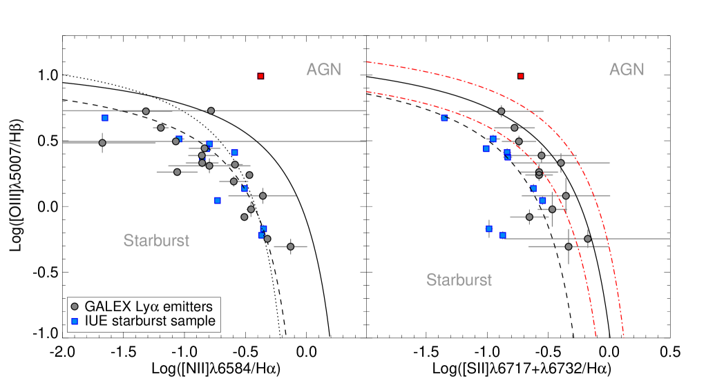
Figure 3: BPT diagrams used to classify narrow emission-line galaxies. GALEX Ly$\alpha$ emitters are represented with black circles with corresponding error bars, together with an IUE sample of local starburst galaxies in blue squares. The left panel show [Oiii] $\lambda 5007$/H$\beta$ versus [Nii] $\lambda 6584$/H$\alpha$ ratios. The dashed and solid curves are theoretical boundaries separating starbursts and AGN objects assuming respectively an instantaneous burst (Dopita et al. 2000) and an extended star formation episode (Kewley et al. 2001). The dotted curve is the “Kauffmann line” (Kauffmann et al. 2003). T͡he right panel represents the [Oiii] $\lambda 5007$/H$\beta$ versus [Sii] ($\lambda 6717+6732$)/H$\alpha$ diagnostic with the same theoretical models as in the right panel. The red dot-dashed shows typical model uncertainties of $\pm$ 0.1 dex. The diagram includes all the 11 IUE local galaxies, amongst which an object previously classified as an AGN (red square) that we decided to show as an example.

3.2 Extinction

In order to measure the gas-phase dust extinction we use the Balmer ratio between H$\alpha$ and H$\beta$. The reddening contribution of our Galaxy is negligible since all our objects are located at high galactic latitude. The extinction coefficient $C(H\beta)$ is then given by the relation:

$$\frac{f(H\alpha)}{f(H\beta)}=B\times 10^{-c[S(H\alpha)-S(H\beta)]}$$ (1)

where f(H$\alpha$) and f(H$\beta$) are the observed fluxes and $B$ is the intrinsic Balmer ratio. We adopted a value of $B=2.86$, assuming a case B recombination theory and a temperature of 10⁴ K (Osterbrock 1989). $S(H\alpha)$ and $S(H\beta)$ are the extinction curve values at H$\alpha$ and H$\beta$ wavelengths respectively and were computed from the Cardelli et al. (1989) extinction law. The reddening $E_{B-V}$ is then simply computed using Eq. 1 and the relation $E(B-V)=c/1.47$. The extinction parameter A_V is derived using a mean ratio of $R=A_{V}/E(B-V)=3.2$.

We will see in Sect. 4.2 and 5 that some galaxies show negative E(B-V). Because we assumed an average correction for the stellar absorption, an overcorrection would lead to an underestimate of the H$\alpha$/H$\beta$ ratio that can explain the few negative values as it can be appreciated from the error bars on the E(B-V) values. In addition, a nebular reflection can also artificially increase the H$\beta$ contribution. In all the following calculations, we assigned E(B-V)=0 to all galaxies showing negative values. However, we show the actual measured values in the plots so the reader can appreciate the uncertainties.

3.3 AGN–Starburst classification

To discuss the nature of the ionizing source in our galaxies, we rely on optical emission line ratios. We examine the [Oiii] $\lambda 5007$/H$\beta$ versus [Nii] $\lambda 6584$/H$\alpha$ diagnostic diagram, also known as the BPT diagram (Baldwin et al. 1981). It allows to distinguish Hii regions photoionized by young stars from regions which photoionization is dominated by a harder radiation field such as that of AGNs or low-ionization nuclear emission-line objects (LINERs). The underlying physics is that because photons from AGNs induce more heating than those of massive stars they will favor the emission from collisionally excited lines with respect to recombination lines. We also use an additional diagram originally proposed by Veilleux & Osterbrock (1987) representing [Oiii] $\lambda 5007$/H$\beta$ versus [Sii] ($\lambda 6717+6732$)/H$\alpha$.

Figure 3 shows the location of our galaxies in these diagrams using dereddened line ratios, although these values are nearly insensitive to dust extinction, and associated uncertainties discussed above. A sample of IUE star forming galaxies in the nearby universe are also shown for comparison. As expected, the points lie in a relatively narrow region highlighting the separation of starburst-like galaxies from other types. In both figures, we have plotted the theoretical curves based on photoionization grids, that leave star forming regions to their lower-left and AGN-type objects to the upper-right. On the left panel, the dashed line represent the upper limit for Hii regions with an instantaneous zero-age star formation model (Dopita et al. 2000), the solid line for an extended burst scenario (more than 4-5 Myr Kewley et al. 2001). The BPT boundary lines are strongly dependent on the effective temperature of the ionizing source, which evolves with time and therefore depends strongly on the star-formation time scale (see for example Cerviño & Mas-Hesse 1994; Kewley et al. 2001). Using a large sample from the sloan digital sky survey (SDSS), Kauffmann et al. (2003) revised this upper limit (plotted with a dotted line) downward. On the right panel we have also plotted the “Dopita and Kewley lines” for the second diagnostic method. However, these models are subject to different uncertainties related to the assumptions made on the chemical abundances, slope of the initial mass function (IMF) or the stellar atmospheres models. The errors on the starburst boundaries may be of the order of 0.1 dex (Kewley et al. 2001). We show in red dash-dotted line, an example of a typical error of 0.1 dex on the [Oiii] $\lambda 5007$/H$\beta$ versus [Sii] ($\lambda 6717+6732$)/H$\alpha$.

We can see that all $z\sim 0.3$ galaxies but one lie on or below the solid starburst division line. This is very clear on the left [Oiii]/H$\beta$ versus [Nii]/H$\alpha$ diagram but proves more ambiguous on the right [Oiii]/H$\beta$ versus [Sii]/H$\alpha$ plot, although this is still consistent with both model and observations uncertainties. The observational uncertainties are particularly important on the right diagram because both redshifted [Sii] $\lambda 6717,6732$ and H$\alpha$ lines are affected by a bright sky background at these wavelengths. Therefore, The BPT diagrams cast doubts on 3 candidates, as objects possibly excited by active nuclei, which we exclude from our analysis. This represents about $\sim 12\%$ of our sample, which is consistent with Cowie et al. (2010) and Scarlata et al. (2009) who find an AGN fraction of 10% and 17%, respectively, in their $z\sim 0.3$ LAE samples. This appears higher than typical AGN fraction ($\sim 0-5\%$) found in high redshift LAE sample (Wang et al. 2004; Gawiser et al. 2006, 2007; Nilsson et al. 2009; Ouchi et al. 2008). Lacking optical spectroscopy, the high-redshift AGN fraction is determined from X-ray data, where the low-luminosity sources comparable to the low-z galaxies might be missed (Finkelstein et al. 2009a). Therefore, this apparent evolution of the AGN fraction might be due to selection effects due to the difficulty to identify AGN in high redshift observations. At low redshift, Finkelstein et al. (2009a) find a significantly higher fraction up to $\sim$ 45% for their LAE sample. There is an overlap of 14 galaxies between the samples of Cowie et al. (2010) and Finkelstein et al. (2009a). Their AGN classification agree on nine of them, while the disagreement for the remaining three stems from, either a discrepancy in the line measurements, i.e. the position in the BPT diagram, or the presence/absence of high-ionization lines. In Particular, object GALEX1421+5239 has been classified as a star-forming galaxy by Cowie et al. (2011) based on the BPT diagram, while Finkelstein et al. (2009a) identified this object (EGS14 in their catalog) as an AGN after the detection of high-ionization lines.

3.4 Oxygen abundance

The determination of the nebular metallicity can give important constraints on the chemical evolution and star formation histories of galaxies. The metal production and the chemical enrichment of the ISM is a direct result of stellar mass build-up and star formation feedback. In addition, the influence of the metal abundance on the evolution of the Ly$\alpha$ output in these galaxies can be investigated.

In order to derive the nebular metallicity of our galaxies we use the optical emission line ratios and different metallicity calibrations according to the lines available in our spectra. For most of our galaxies, we measure the widely used abundance indicator, the $R_{23}$ index, which is based on the ratio ([Oii] $\lambda$3727 + [Oiii] $\lambda\lambda$ 4959,5007)/H$\beta$ (Pagel et al. 1979; McGaugh 1991; Kobulnicky et al. 1999; Pilyugin 2003). The main problem with the relationship (O/H)-$R_{23}$ is that there is a turnover around 12 + log(O/H) $\sim$ 8.4 that makes this index double-valued. A given $R_{23}$ value could correspond to a high or low metallicity. Kewley & Ellison (2008) have shown that additional line ratios such as [Nii]/[Oii] or [Nii]/H$\alpha$ can be used to break this degeneracy. We used the [Nii]/[Oii] ratio to determine which of the upper and lower branch of the metallicity calibration to use.

Several studies have demonstrated that the $R_{23}$ method generally overestimates the actual metallicity when compared to the direct method (e.g. Kennicutt et al. 2003; Bresolin et al. 2005; Yin et al. 2007). This discrepancy prevents us from having an accurate measurement with $R_{23}$ for intermediate metallicities, i.e. around the turnover region. Therefore, we here turn to other metallicity indicators that give more consistent results. We first use the emission-line ratio Log([Nii]$\lambda$6583/H$\alpha$), known as the $N2$ index (Denicoló et al. 2002; Pettini & Pagel 2004). The calibration of this indicator has been derived from the comparison of (O/H) measured using the “direct” method (via the electron temperature $T_{e}$), and the $N2$ index in a large sample of extragalactic Hii regions. They obtain the relationship that translates $N2$ to oxygen abundance, 12 + log (O/H) $=8.90+0.57\times N2$. Then, we consider the $O3N2$ index originally introduced by Alloin et al. (1979), which corresponds to the line ratio Log{([Oiii] $\lambda$5007/H$\beta$)/([Nii] $\lambda$ 6583/H$\alpha$)}. Pettini & Pagel (2004) used a sub-sample of their Hii regions to produce a calibration for this indicator and found a best fit with 12 + Log (O/H) $=8.73-0.32\times O3N2$. However this relationship is only valid for galaxies with $O3N2<2$, which is the cases for our galaxies. Of our sample of 21 galaxies, we were able to perform these metallicity measurements for 20 of them (for the remaining one the quality of the spectrum is not sufficient to confidently measure emission line fluxes), and for all of the 10 IUE galaxies.

It is well known that the $R_{23}$ and other indicators are sensitive to the ionization parameter, and applying the above calibration to our sample assumes no variation in the ionization state, which can lead to inaccurate metallicity estimates. A detailed discussion about the effects of the ionization parameter on the different metallicity indicators has been presented in several studies using photoionization models (see for example Cerviño & Mas-Hesse 1994; Kewley & Dopita 2002). When $Z<0.5Z_{\odot}$, i.e. 12 + log (O/H) $\lesssim 8.6$, an increasing ionization parameter corresponds to an increasing value of the $R_{23}$ index, and inversely for metallicities higher than 0.5 $Z_{\odot}$ (see Fig. 5 in Kewley & Dopita 2002). For single-valued indicators, the index increases with increasing ionization parameter. However, for their sample of $z\sim 0.3$ galaxies, Cowie et al. (2011) determined the metallicity using the “direct” method thanks to the detection of the [Oiii]$\lambda$4363, and compared the results to the $N2$ indicator. They found a good correlation with small scatter indicating relatively small effects from the ionization parameter. Moreover, while the absolute value of the metallicity may suffer from uncertainties, the trends analyzed here should hold irrespective of the absolute values, given the small range of metallicities covered by the sample.

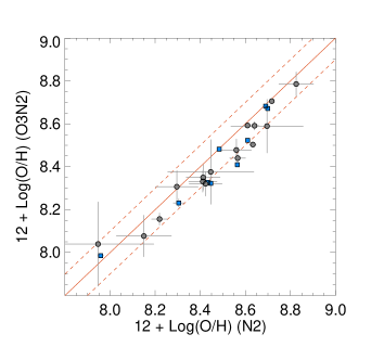
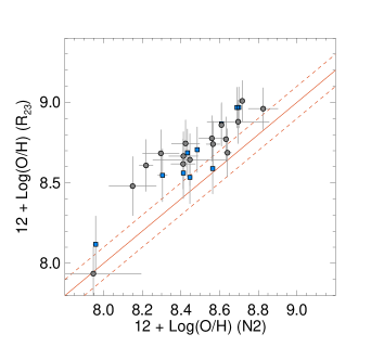
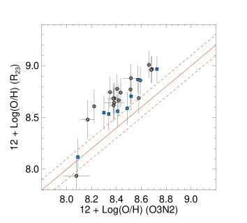
Figure 4: Comparison between the oxygen abundances derived different indicators: R₂₃= ([Oii] $\lambda$3727 + [Oiii] $\lambda\lambda$ 4959,5007)/H$\beta$ (Pagel et al. 1979), $N2$ = Log([Nii]$\lambda$6583/H$\alpha$) and $O3N2$ = Log{([Oiii] $\lambda$5007/H$\beta$)/([Nii] $\lambda$ 6583/H$\alpha$)} (Pettini & Pagel 2004). The $z\sim 0.3$ galaxies are shown with black circles and the local galaxies with blue squares with 1$\sigma$ error bars. The solid line represents the 1:1 ratio with $\pm$0.1 dex uncertainties (dashed lines). Note that some galaxies are not present in all the plots because the corresponding diagnostic lines were not detected with a sufficient significance.

We show in Fig. 4 a comparison between the oxygen abundance derived from several indicators: R₂₃,$N2$, and $O3N2$. It appears that $N2$ and $O3N2$ are in good agreement, although the values derived from $O3N2$ are systematically lower by 0.1 dex on average than those of the $N2$ method. On the other hand, although we do not have a direct measurement of the metallicity, we confirm that $R_{23}$ index overestimates the oxygen abundance by a factor up to 0.4 dex when compared to the two other methods used here. The $N2$ index is used in the rest of this analysis when it is available, otherwise $O3N2$ is adopted.

4 The regulatory factors of the Ly$\alpha$ output in galaxies

4.1 Effects of metallicity

The first detections of the Ly$\alpha$ emission line in star-forming galaxies goes back to the early IUE observations of nearby Hii galaxies (e.g. Meier & Terlevich 1981; Hartmann et al. 1984; Deharveng et al. 1985). However, in the case of detection, the line was very weak, while in the remaining galaxies it was found in absorprtion. The most natural explanation was the attenuation of the Ly$\alpha$ photons by dust. The metallicity was often used as a dust indicator and compared with the Ly$\alpha$ strength. The study of small galaxy samples (Meier & Terlevich 1981; Terlevich et al. 1993; Charlot & Fall 1993) shows an anti-correlation between $EW_{\mathrm{Ly}\alpha}$ and the metallicity, whereas the more comprehensive results of Giavalisco et al. (1996) show only a marginal trend.

Here we investigate the effects of the metallicity on Ly$\alpha$ emission in a large sample of galaxies. While the metallicity can be correlated with the H$\alpha$ equivalent width as the result of metal enrichment with the age of the galaxy, this is not necessarily the case for the Ly$\alpha$ strength. Cowie et al. (2011) compared the metallicity of a LAE sample and UV-selected galaxies and found that galaxies without Ly$\alpha$ tend to have median metallicities 0.4 higher. Finkelstein et al. (2011b) also show that LAEs at low redshift have lower metallicities than similar-mass galaxies from the SDSS. One may expect a strong intrinsic Ly$\alpha$ emission for a low-metallicity galaxy but the observed Ly$\alpha$ output will also depend on other factors. Classical examples are IZw 18 and SBS 0335, the most metal-poor galaxies known, that show a strong absorption in Ly$\alpha$ (Kunth et al. 1998; Mas-Hesse et al. 2003; Atek et al. 2009b). In fact, the metallicity distributions of the LAEs and UV-continuum galaxies measured in Cowie et al. (2011) overlap significantly. Figure 5 shows how Ly$\alpha$ equivalent width is uncorrelated with the oxygen abundance. This means in particular that strong Ly$\alpha$ emitters are not systematically metal-poor galaxies.

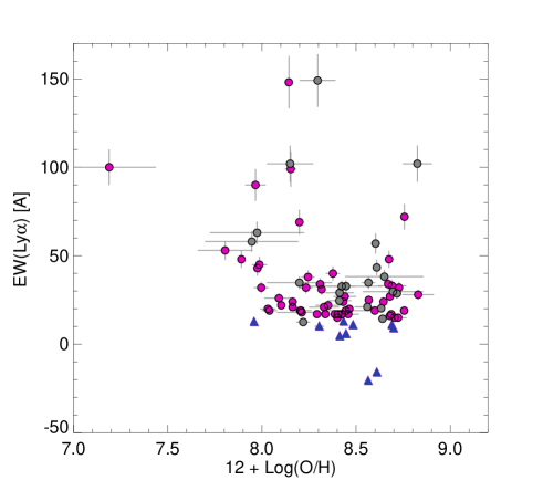
Figure 5: The Ly$\alpha$ equivalent with as a function of metallicity. The oxygen abundance is derived from the $N2$ index Log([Nii]$\lambda$6583/H$\alpha$) using the equation of Pettini & Pagel (2004). The present sample is shown with black circles, Cowie et al. (2011) galaxies with magenta circles, and IUE galaxies with blue triangles.

4.2 Effects of dust

As detailed in Sect. 3.2, we have derived the dust extinction in the gas phase from the Balmer decrement H$\alpha$/H$\beta$ for all the galaxies studied here. Previous investigations concerning the effects of dust on the Ly$\alpha$ emission, and in particular the correlation between the Ly$\alpha$ equivalent width and extinction, have interestingly led to different results and conclusions. Giavalisco et al. (1996) found a large scatter in the correlation between $EW_{\mathrm{Ly}\alpha}$ and the color excess $E(B-V)$ in a sample of 22 nearby starbursts. They concluded that, in addition to resonance scattering effects, Ly$\alpha$  escape may be affected by the geometry of the neutral phase of the ISM, such as patchy dusty regions or ionized holes. However, these results stand in contrast with high redshift studies of Ly$\alpha$ emitters. Composite spectra of $z\sim 3$ LBGs (Shapley et al. 2003) showed a trend between $EW_{\mathrm{Ly}\alpha}$ and $E(B-V)$ where objects with strong Ly$\alpha$ emission have also steeper UV continuum. Similar trends have been observed more recently (Vanzella et al. 2009; Pentericci et al. 2009; Kornei et al. 2010) where LBGs that exhibit Ly$\alpha$ in emission tend to have bluer UV slopes than those with Ly$\alpha$ in absorption. Following Shapley et al. (2003), Pentericci et al. (2009) separated their $z\sim 4$ LBG sample in bins of extinction and noted same trend between the mean values of $EW_{\mathrm{Ly}\alpha}$ versus stellar extinction. Again, all the observed correlations listed here are model-dependent, and may be affected by several uncertainties. Differences in the inferred physical properties may arise from the different extinction laws adopted in those studies, such as Calzetti et al. (2000) vs SMC (Prevot et al. 1984), which depends also on the age and the redshift of the galaxies (Reddy et al. 2006; Siana et al. 2009). More generally, the choice of a specific IMF and metallicity, or the degeneracy between age and extinction may introduce systematic uncertainties. Finally, as discussed in Hayes et al. (2013), the IUE aperture at $z\sim 0.01$ probes a much smaller physical size than other studies at higher redshift. For lower dust extinction, Ly$\alpha$ is spatially more extended leading to aperture losses, hence an underestimation of the Ly$\alpha$ escape fraction.

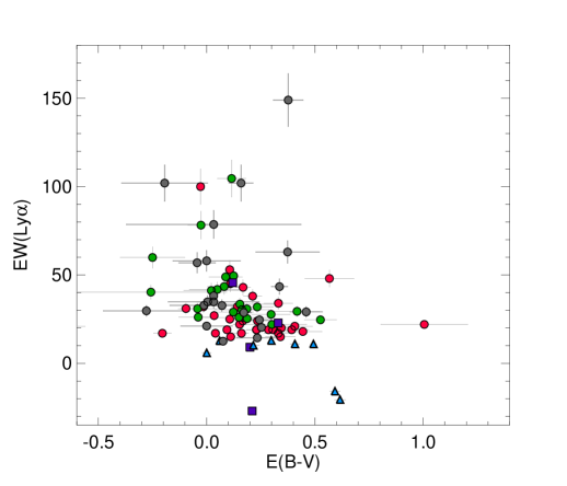
Figure 6: The Ly$\alpha$ equivalent width as a function of the gas-phase dust extinction. Black circles are the GALEX Ly$\alpha$ emitters, green and red circles are the other GALEX samples of Scarlata et al. (2009) and Cowie et al. (2011), respectively. The blue triangles represent the IUE spectroscopic sample, and purple squares local starbursts from Atek et al. (2008).

Figure 6 shows $EW_{\mathrm{Ly}\alpha}$ as a function of the extinction. The plot includes a compilation of local starbursts and $z\sim 0.3$ GALEX-selected samples. The published values of Cowie et al. (2011) are in bins of flux, which explains the discrete positions of E(B-V) for this sample. The Ly$\alpha$ equivalent width shows a large scatter for $E(B-V)$ ranging from no extinction to $\sim 0.45$. This is consistent with previous results of Ly$\alpha$ imaging observations of local starbursts (Atek et al. 2008; Östlin et al. 2009), of which data points are plotted on the figure (purple squares). The dispersion of Ly$\alpha$ strength observed for a given value of extinction is indicative of the influence of other galaxy parameters besides pure dust attenuation, such as Hi column density that may increase the suppression of Ly$\alpha$ or neutral gas outflow that may ease the escape of Ly$\alpha$ photons. However, as previously shown by Schaerer & Verhamme (2008); Verhamme et al. (2008); Atek et al. (2009b), the effects of superwinds might become insufficient in the case of high extinction, in which case we observe Ly$\alpha$ in absorption or with a low equivalent width. This can be observed in Fig. 6 where no high $EW_{\mathrm{Ly}\alpha}$ values can be observed for large extinctions.

The absence of anti-correlation between EW_Lyα and E(B-V) can be attributed to the difference in the type of extinction probed. While the stellar extinction is responsible for continuum attenuation, the Ly$\alpha$ line flux is affected by the nebular extinction around the recombination regions. Therefore, the quantity of dust, and more importantly, the geometry of the dust distribution, can be very different between the two phases. In that case, the total extinction we derive from integrated fluxes would not be representative of the ”effective” extinction affecting each radiation, and the total E(B-V) could become meaningless for very high extinction. We show in Table 3 the extinction factor at $\lambda$ = 1216 Å for different E(B-V) values and two extinction laws (Cardelli et al. 1989; Prevot et al. 1984). As we can see, for E(B-V) values above 0.3, we could hardly detect any UV continuum nor Ly$\alpha$ emission, since the extinction factor becomes rapidly higher than 100. At E(B-V) $\sim 1$, photons in the UV domain should be completely absorbed, which stands in contrast with $EW_{\mathrm{Ly}\alpha}$ values around 50 Å observed at such extinction levels. This suggests two mechanisms: (i) because of their resonant scattering, Ly$\alpha$ photons can spatially diffuse far from the ionized regions where the Balmer lines are produced (from which we measure the extinction) and will sample different extinction, (ii) in the optical domain we will sample deeper regions and derive large average E(B-V) values, while in the UV, the observations are dominated by the contribution of the few stars/regions with lower values of extinction. Deeper regions would be completely obscured and would not contribute significantly in the UV. As a result, the average E(B-V) value in the UV (both Ly$\alpha$ and continuum), would be much lower than in the optical (see Otí-Floranes et al. 2012, for a detailed discussion about the differential extinction). In Sect. 5, we will also investigate the effects of the differential extinction scenario on the Ly$\alpha$ escape fraction.

Table 3: Extinction factors at $\lambda$ = 1216 Å, calculated for different values of E(B-V) using the Galactic extinction (Cardelli et al. 1989) and the SMC law (Prevot et al. 1984).

E(B-V)	0.1	0.2	0.3	0.5	1
Cardelli et al. (1989)	0.37	0.14	0.05	7$\times 10^{-3}$	5$\times 10^{-5}$
Prevot et al. (1984)	0.19	0.04	7$\times 10^{-3}$	2$\times 10^{-4}$	6$\times 10^{-8}$

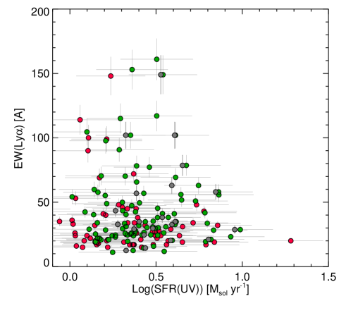
Figure 7: $EW_{\mathrm{Ly}\alpha}$ as a function of UV star formation rate. The color-code is the same as Fig. 6

. The Ly$\alpha$ equivalent width is the observed rest-frame value and the SFR_UV values are calculated from FUV luminosity at 1530 Å not corrected for extinction. $EW_{\mathrm{Ly}\alpha}$ uncertainties are 10% error bars, and SFR_UV errors are derived from GALEX FUV photometry.

4.3 Ly$\alpha$ equivalent width as a function of UV luminosity

With the aim of understanding the different parameters governing the Ly$\alpha$ escape and observability, many studies, both observational and theoretical, have found an apparent variation of the Ly$\alpha$ strength with the UV luminosity (Shapley et al. 2003; Ando et al. 2006; Ouchi et al. 2008; Verhamme et al. 2008; Vanzella et al. 2009; Pentericci et al. 2009; Balestra et al. 2010; Stark et al. 2010; Schaerer et al. 2011; Shimizu et al. 2011). In particular, the data show a lack of high Ly$\alpha$ equivalent width in luminous LBGs. A well known trend is the decrease of $EW_{\mathrm{Ly}\alpha}$ with SFR_UV (Ando et al. 2004; Tapken et al. 2007; Verhamme et al. 2008). At higher redshift, Stark et al. (2010) found that galaxies with strong Ly$\alpha$ emitters have smaller UV luminosities, and have in general a bluer UV slope compared to galaxies with weak Ly$\alpha$ emission. A similar plot is shown in Fig. 7. Although, the correlation presented in Verhamme et al. (2008) or Stark et al. (2010) cover a larger range in both SFR_UV and $EW_{\mathrm{Ly}\alpha}$, our data do not show such a clear trend, but rather an $EW_{\mathrm{Ly}\alpha}$ distribution independent of UV luminosity. Together, Fig. 6 and 7 indicate that the difference in the type of extinction probed combined with complex transport of Ly$\alpha$ make the picture difficult to interpret. While the stellar extinction is responsible for continuum attenuation, the line flux is affected by the nebular extinction around the recombination regions combined to gas outflows. Therefore, the quantity of dust, and more importantly, the geometry of the dust distribution, can be very different between the two phases, and therefore between the continuum and the line behaviour. The absence of strong Ly$\alpha$ emission at high SFR(UV) observed in high-$z$ samples can be due to differences in star formation histories and time scales, rather than an increase of the dust content, because powerful instantaneous bursts that produce very high $EW_{\mathrm{Ly}\alpha}$ are more likely at young ages, i.e. small SFR_UV, and constant star formation episodes at later stage characterized by modest $EW_{\mathrm{Ly}\alpha}$ at equilibrium.

5 The Ly$\alpha$ Escape Fraction

In Atek et al. (2009a), we presented an empirical estimate of the Ly$\alpha$ escape fraction in a large sample of galaxies selected from GALEX spectroscopy (Deharveng et al. 2008). Here we derive $f_{esc}$(Ly$\alpha$) for two additional $z\sim 0.3$ galaxy samples of Scarlata et al. (2009) and Cowie et al. (2011). The Ly$\alpha$ escape fraction is calculated following the equation:

$$f_{esc}(\mathrm{Ly}\alpha)=f(\mathrm{Ly}\alpha)/(8.7\times f(\mathrm{H}\alpha)_{C}),$$ (2)

where $f$(Ly$\alpha$) is the observed flux and $f$(H$\alpha$)_C is the extinction-corrected H$\alpha$ flux. The recombination theory (case B) gives a an intrinsic ratio of $f$(Ly$\alpha$)/$f$(H$\alpha$) = 8.7 (Brocklehurst 1971). The Cowie et al. data were obtained with a 1″ slit, while Scarlata et al. used a 1.5″slit. These measurements are not well matched to the GALEX aperture and can suffer from systematic errors. Both groups used a larger aperture for only few galaxies in their samples, and only to assess the importance of aperture effects. Scarlata et al. (2009) used a 5″slit for eight targets and compared the results with those made in the narrow slit, finding errors up to 25 %. For the same reason, Cowie et al. (2011) compared their measurements in the narrow and wide slits with those of Scarlata et al. (2009) for a subset of galaxies that overlap, and they found a general agreement for their line fluxes. However in some cases the differences were important reaching a factor of 2 or more. We note that those large aperture measurements were not used in their analysis. If this is the case for some of our galaxies, we would overestimate their $f_{esc}$(Ly$\alpha$) values. Two effects can lead to inaccurate measurements of $f_{esc}$(Ly$\alpha$): (i) if the dust is not uniformly distributed across the galaxy, targeting only the central part of the galaxy would produce systematic error on E(B-V). (ii) The spatial extension of the H$\alpha$ emission can go well beyond the size of the narrow slit, which results in an underestimate of the total H$\alpha$ flux that should match the total Ly$\alpha$ flux from GALEX. In order to better quantify these two effects on our results, we compared our measurements in 1″and 5″slits. We found that the dust reddening E(B-V) tends to be overestimated by a factor of 1.5 in the narrow slit, which possibly means the dust amount is higher in the center of the galaxy. Regarding H$\alpha$ emission, we first corrected both observed H$\alpha$ fluxes using the E(B-V) calculated in their respective slits. We found that the intrinsic H$\alpha$ flux is underestimated by 30% on average when using the narrow slit. We therefore applied these aperture correction factors to the samples of Scarlata et al. (2009) and Cowie et al. (2011). The effect of such a correction is to increase the intrinsic H$\alpha$ flux, and hence to decrease the Ly$\alpha$ escape fraction. However, this does not have a significant impact on our results because Log($f_{esc}$_,Lyα) is revised by only $\sim$0.1 on average, and the observed trends remain unchanged (eg. the correlation between Log($f_{esc}$_,Lyα) and E(B-V)). Another difference is that, unlike the Scarlata et al. sample, Cowie et al. did not apply any stellar absorption to their emission lines. However, the median value for their H$\alpha$ equivalent width is $\sim 80\AA$. A typical correction of 2Å is then negligible and introduces a much smaller errors than the slit loss problems discussed above. Finally, we show in Fig. 8 a comparison between the $EW_{\mathrm{Ly}\alpha}$ distribution of our sample and those of Cowie et al. and Scarlata et al. We note that the distribution of our sample is shifted to higher $EW_{\mathrm{Ly}\alpha}$ compared to that of Cowie et al. which peaks at small $EW_{\mathrm{Ly}\alpha}$ (less than 20 Å). This is the result of our selection in the Deharveng et al. sample of good quality Ly$\alpha$ lines only which favors high $EW_{\mathrm{Ly}\alpha}$. This will also result in selecting relatively higher Ly$\alpha$ escape fraction as we will see later.

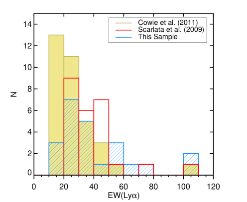
Figure 8: Ly$\alpha$ equivalent width distribution for the three GALEX samples used in this work. It includes all sources with optical follow-up spectroscopy.

We first show in Fig. 9, that the Ly$\alpha$ escape fraction is not correlated to the oxygen abundance. This is similar to what we have seen in section 4.1. It indicates that the metal abundance is not an important regulatory factor of the Ly$\alpha$ escape.

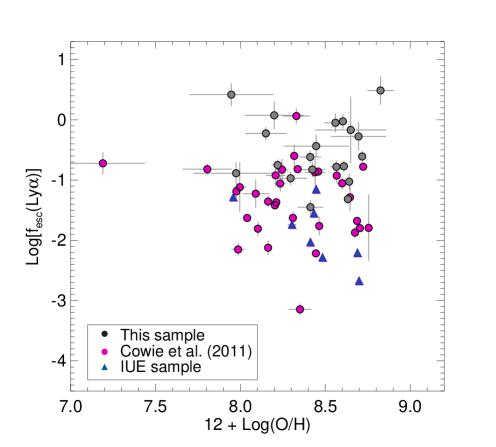
Figure 9: The Ly$\alpha$ escape fraction as a function of the gas-phase metallicity. The oxygen abundance is derived from the $N2$ index Log([Nii]$\lambda$6583/H$\alpha$) using the equation of Pettini & Pagel (2004). The color code as the same as in Fig. 5

We present on the left side of Figure 10 the relation between $f_{esc}$(Ly$\alpha$) and the gas-phase extinction. The color-code for the different samples is presented in the legend. We fitted the Log($f_{esc}$)-E(B-V) correlation using the MPFITEXY IDL routine (Williams et al. 2010) which is based on MPFIT procedure (Markwardt 2009). The routine fits the best straight line to the data taking into account the errors in both X and Y directions. The black solid line represents the best fit to the function $f_{esc}$(Ly$\alpha$)$=C_{Ly\alpha}\times 10^{-0.4\leavevmode\nobreak\ E(B-V)\leavevmode\nobreak\ k_{Ly\alpha}}$ where the origin C_Lyα and the slope $k_{Ly\alpha}$ are left as free parameters. Overall, the figure confirms the decreasing trend of $f_{esc}$(Ly$\alpha$) with increasing extinction observed in several studies (Atek et al. 2008, 2009a; Verhamme et al. 2008; Kornei et al. 2010; Hayes et al. 2010, 2011). However, when the origin is fixed at C${}_{Ly\alpha}=1$, i.e. assuming $f_{esc}$(Ly$\alpha$)=1 in the absence of dust, we derive an extinction coefficient of $k_{Ly\alpha}\sim 11.3\pm 0.7$, which is slightly higher than what would be expected if dust extinction were the only factor affecting Ly$\alpha$ escape, $k_{1216}=9.9$ assuming a Cardelli et al. (1989) extinction law (the dot-dashed line).

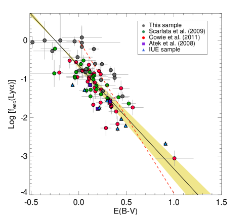
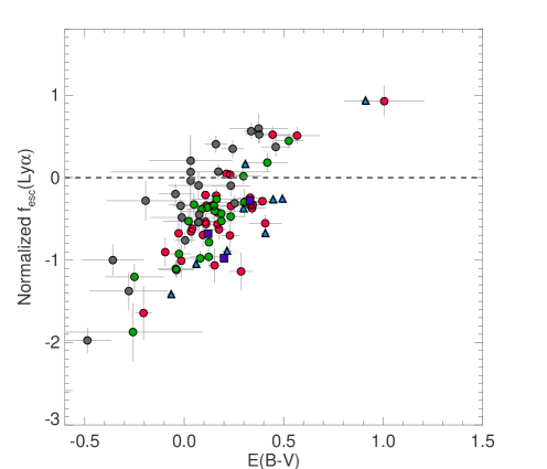
Figure 10: Ly$\alpha$ escape fraction as a function of the nebular dust extinction. The figure shows the $z\sim 0.3$ Ly$\alpha$ emitters of this work with black circles. We also derived $f_{esc}$(Ly$\alpha$) for other galaxy samples: $z\sim 0$ IUE sample represented by blue triangles, $z\sim 0.3$ sample of Scarlata et al. (2009) with green circles, Cowie et al. (2011) sample with red circles, $z\sim 0$ galaxies of Atek et al. (2008) with purple squares. Note that the negative values of E(B-V) are shown in the plot but were assigned E(B-V)=0 before $f_{esc}$(Ly$\alpha$) calculation or fitting the $f_{esc}$-E(B-V) relationship. The left panel shows $f_{esc}$(Ly$\alpha$) as a function of E(B-V) assuming a Cardelli et al. (1989) extinction law. The solid black line denotes the best 2-parameter fit to the relationship with both the slope and the intercept as free parameters. The yellow region covers the 1$\sigma$ uncertainties of the fit derived from MC simulations. The dashed red line is the expected attenuation law at the Ly$\alpha$ wavelength. In the right panel we plot the normalized escape fraction $f_{esc}$_,rel(Ly$\alpha$)=log[$f_{esc}$(Ly$\alpha$)/$f_{esc}$(cont)] as a function of extinction. The normalized escape fraction represents the deviation of $f_{esc}$(Ly$\alpha$) from the classical dust attenuation law at 1216 Å. The color code for the samples is the same as in the left panel.

In the case of a 2-parameter fit, we find $k_{Ly\alpha}\sim 6.67\pm 0.52$ and C${}_{Ly\alpha}=0.22\pm 0.03$. The fit is shown by the solid black line in Fig. 10 while the uncertainties are represented by the shaded yellow region. To estimate the errors on the fit, we performed Monte Carlo simulations by generating a sample of 1000 datasets by randomly varying $f_{esc}$(Ly$\alpha$) and E(B-V) within their respective uncertainties. Then, we used the same procedure to fit each dataset. The two-parameter fit shows that even when no dust is present, the Ly$\alpha$ emission is still attenuated by resonant scattering and the geometrical configuration of the ISM. Removing object GALEX1421+5239, which might be an AGN (cf. Sect. 3.3), results in a slightly higher extinction coefficient with $k_{Ly\alpha}\sim 6.73$. Hayes et al. (2011) used the same prescription to describe the effects of dust on the Ly$\alpha$ escape fraction in a compilation of galaxies at redshift $z\sim 2$. However, the E(B-V) was derived from full SED fitting, and $f_{esc}$(Ly$\alpha$) was based either on the UV continuum or the H$\alpha$ line corrected for extinction using the stellar E(B-V). After fitting the $f_{esc}$(Ly$\alpha$)-E(B-V) relation, they obtained $k_{Ly\alpha}\sim 13.8$ and C${}_{Ly\alpha}=0.445$, assuming a Calzetti et al. (2000) extinction law. Compared to these values, we obtain a smaller extinction coefficient $k_{Ly\alpha}$ and a lower intercept point at zero extinction. Here we draw attention to selection effects that can possibly contribute to the observed differences. The $z\sim 0.3$ LAEs detected by GALEX were selected based on a relatively strong Ly$\alpha$ emission, which is therefore biased towards high Ly$\alpha$ escape fractions. In the case of the $z\sim 2$ sample, galaxies were mostly selected upon their UV continuum or H$\alpha$ emission. In fact, it has been shown in Hayes et al. (2010) that Ly$\alpha$- selected galaxies have higher $f_{esc}$(Ly$\alpha$) values than H$\alpha$-selected ones.

While the dust-dependence of $f_{esc}$(Ly$\alpha$) is clear, it does not follow classical dust attenuation prescriptions because of secondary parameters at play. In the right panel of Figure 10, we illustrate the deviation of $f_{esc}$(Ly$\alpha$) from the value expected from E(B-V) under standard assumptions by plotting the normalized escape fraction defined as:

$$f_{esc}^{norm}(Ly\alpha)=f_{esc}(Ly\alpha)/f_{esc}(cont_{1216})$$ (3)

where, $f_{esc}$(Ly$\alpha$) is the Ly$\alpha$ escape fraction and $f_{esc}(cont_{1216})$ is the escape fraction of the UV continuum at 1216 Å. The dashed horizontal line indicates the case where the Ly$\alpha$ emission obeys to the same attenuation law as the UV continuum radiation. The values of $f_{esc}$(Ly$\alpha$) below this line can be explained by the the scattering of Ly$\alpha$ photons in the neutral gas, which increases their optical path, thus the extinction coefficient. $f_{esc}$(Ly$\alpha$) values above the upper limit driven by the nebular dust extinction could be attributed to several physical processes or any combination thereof. First, the geometry of the ISM can change the behavior of Ly$\alpha$ photons with respect to dust attenuation. In the case of a multi-phase ISM, where the neutral gas and dust reside in small clouds within an ionized inter-cloud medium, Ly$\alpha$ photons scatter off of the surface of the clouds to escape easier than non-resonant photons that enter the clouds to encounter dust grains (Neufeld 1991; Hansen & Peng Oh 2006; Finkelstein et al. 2008). Therefore, the preferential escape of Ly$\alpha$ increases with increasing extinction, which is observed in our case. Finkelstein et al. (2011a) investigated the effects of ISM geometry on the Ly$\alpha$ escape in a sample of 12 LAEs. Five of their galaxies where consistent with an enhancement of the observed $EW_{\mathrm{Ly}\alpha}$. Laursen et al. (2012) and Duval et al. (2013) recently discussed the scenario of multi-phase ISM scenario to explain unusually high Ly$\alpha$ equivalent widths observed in high-$z$ LAEs. Their models show that very specific and restrictive conditions are needed in order to enhance the intrinsic EW(Ly$\alpha$), such as a high extinction and a low expansion velocity. Always in the context of a peculiar ISM geometry, Scarlata et al. (2009) discussed the possibility of a different effective attenuation resulting from a clumpy ISM (Natta & Panagia 1984), which does not take the classical e^-τ form but will depend on the number of clumps. This can reproduce the Ly$\alpha$ enhancement observed in the objects above the dashed line. Given the increase of $f_{esc}^{norm}$ with increasing extinction, it is possible that the two mechanisms (enhancement of Ly$\alpha$ by scattering and a peculiar extinction law) are at play, as they both require a high extinction to significantly increase the escape of Ly$\alpha$. If we go beyond the simplistic spherical geometry, more realistic configurations of the ISM could also favor Ly$\alpha$ transmission. Ionized cones along the observer’s sightline can preferentially transmit Ly$\alpha$ photons via channeling, i.e. scattering of Ly$\alpha$ photons on the Hi outskirts along the cone. Moreover, the Ly$\alpha$ strength depends also on the inclination of the galaxy. Because Ly$\alpha$ photons will follow the path of least opacity they will preferentially escape face-on. This is not necessarily the case for H$\alpha$ photons which don’t undergo an important angular redistribution (Verhamme et al. 2012).

More generally, as we have shown in Sect. 4.2, when the extinction is high enough (typically E(B-V) $>0.3$), the differential extinction sampling would naturally produce $f_{esc}^{norm}$ values higher than one. In the Hii regions affected by dust, $f_{esc}$(Ly$\alpha$) will be very low, while in the dust-free regions, where the Ly$\alpha$ emission will dominate the rest of Balmer lines, $f_{esc}^{norm}$ will be higher than unity, since the total E(B-V) derived does not apply to those regions. In summary, if one expect starburst galaxies to have a gradation of extinction in different parts of the Hii regions, from regions completely onscured in the UV to regions almost devoid of dust, the convolution of all regions would give an evolution of $f_{esc}^{norm}$ with average E(B-V) similar to the diagram shown in Fig. 10.

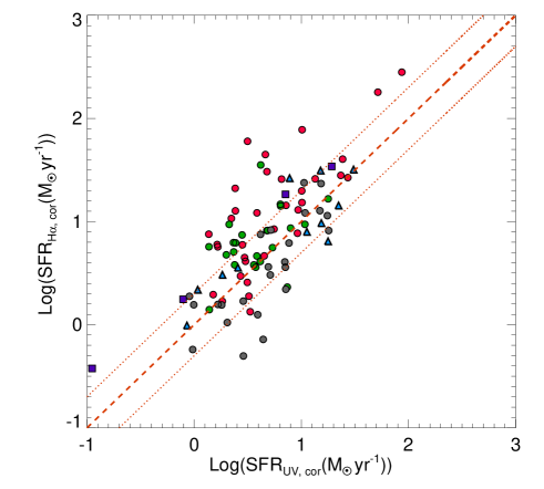
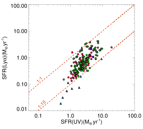
Figure 11: Comparison between SFR indicators. The SFR values are calculated using Kennicutt (1998) calibration. The left panel shows SFR(H$\alpha$) versus SFR(UV) both corrected for dust extinction derived from the Balmer decrement. The dashed line denotes the line of equality, while the dotted lines have a factor of 2 deviation. The right panel presents the observed SFR(Ly$\alpha$) as a function of SFR(UV), with no correction for dust extinction. The two dashed lines marks the 1:1 and 1:10 ratios for SFR_Lyα:SFR_UV. The symbols are the same as in Fig. 10.

Another possible source of the Ly$\alpha$ excess is collisional excitation. If the electron temperature is high enough (typically higher than $\sim 2\times 10^{4}$ K), collisions with thermal electrons lead to excitation and then radiative de-excitation. This process becomes non negligible compared to the recombination source in the case of high ISM temperatures. Furthermore, it has been suggested that a weak component of Ly$\alpha$ emission can originate from ionization by the plasma of very-hot X-ray emitting filaments, as Otí-Floranes et al. (2012) observed a spatial correlation between the soft X-ray emission and the diffuse Ly$\alpha$ component in the galaxy Haro 2. Given the small values of $f_{esc}$(Ly$\alpha$) that show a significant Ly$\alpha$ enhancement, i.e. $f_{esc}$(Ly$\alpha$) $<5\%$ for $f_{esc}^{norm}$(Ly$\alpha$) $>1$, one needs a relatively small contribution from the other emission processes to reproduce the deviation from expected attenuation by dust.

6 Ly$\alpha$ as a star formation rate indicator

In view of the important role that the Ly$\alpha$ line will plays in the exploration of the distant universe with the upcoming new generation of telescopes such as the JWST and the ELTs, it is essential to know to what extent the observed Ly$\alpha$ flux is representative of the intrinsic emission. The key capability for the detection of galaxies at $z>7$ will be the rest-frame UV emission and, in the case of faint galaxies, the strongest emission line Ly$\alpha$. Typical high-redshift emission-line surveys rely on the strength of the Ly$\alpha$ line, which is usually observed on top of a faint continuum. However, the interpretation of this line is hampered by many uncertainties related to complex transmission through the ISM and the IGM.

In Figure 11, we first compare the SFR derived from H$\alpha$ with the one based on the UV. Both quantities were corrected for dust extinction, were the stellar extinction affecting the UV continuum was assumed to be a factor of 2 lower than the gas phase extinction derived from the H$\alpha$/H$\beta$ ratio (Calzetti et al. 2000). The H$\alpha$ emission is the result of the recombination of hydrogen atoms that have been previously ionized by the radiation of hot OB stars which have short lifetimes. It traces therefore the quasi instantaneous star formation rate on the scale of few Myrs. The UV (non ionizing) radiation is also emitted by less massive galaxies with longer life times – typically few Gyrs – and is indicative of the averaged SFR over the galaxy lifetime. We can see that the two SFR indicators are in broad agreement with a significant dispersion. Small differences are actually expected due to different star formation histories traced by these two emissions (cf. Kennicutt 1998; Schaerer 2003)

In order to assess the reliability of Ly$\alpha$ as tracer of star formation, we now compare the SFR(Ly$\alpha$) with SFR(UV). The result is presented in the right panel of Fig. 11, which shows the observed SFRs derived using the Kennicutt (1998) calibrations. The two dashed lines represent the ratios SFR_UV/SFR_Lyα = 1 and 10. We see that the Ly$\alpha$ indicator clearly underestimates the SFR when compared with the UV indicator. This is consistent with the discrepancy found in most of high-$z$ observations (e.g. Yamada et al. 2005; Taniguchi et al. 2005; Gronwall et al. 2007; Tapken et al. 2007; Guaita et al. 2010). We note that the correction of SFR(Ly$\alpha$) with $f_{esc}$(Ly$\alpha$) gives a good estimate of the true SFR since it becomes equivalent to plotting SFR(H$\alpha$), given the definition of $f_{esc}$(Ly$\alpha$) (cf. Equation 2). However, obtaining the Ly$\alpha$ escape fraction for high-$z$ galaxies remains very challenging.

We now compare the deviation of SFR(Ly$\alpha$) from the true SFR (which is assumed to be SFR(UV)) as a function of SFR(UV). The idea is to know when the observed Ly$\alpha$ flux can be used as an SFR measurement. We plot in Figure 12 the logarithm of the observed ratio SFR_Lyα/SFR_UV as a function of SFR_UV. It is important here to compare our results to the high-z studies available in the literature. For this reason, we included in the plot of Fig. 12 additional samples described in the caption from $z\sim 2$ to $z\sim 6$. For reference, the dashed horizontal line represents the 1:1 ratio for SFR_UV/SFR_Lyα. The yellow region represents the range of values of SFR_UV/SFR_Lyα that would be retrieved for different star formation histories, when the standard calibration from Kennicutt (1998) is used (this calibration is based on the case of an evolved starburst already in its equilibrium phase). For a young burst or constant star formation that hasn’t reached equilibrium yet (age $<100$ Myr), SFR(Ly$\alpha$) is higher than SFR(UV), and a ratio of SFR_Lyα/SFR_UV $\sim 4$ can be observed (Schaerer 2003; Verhamme et al. 2008), which is represented by the upper part of the yellow region. For older galaxies ($>$ 1 Gyr) with a constant star formation history, SFR(UV) becomes higher than SFR(Ly$\alpha$), which explains the lower part of the yellow region.

Clearly, the SFR measured from Ly$\alpha$ is most of the time, and at all redshifts, lower than the true SFR. We can observe a general decline of the SFR_Lyα/SFR_UV with increasing SFR_UV. As discussed for Fig. 7 describing the decrease of $EW_{\mathrm{Ly}\alpha}$ as a function of SFR_UV, this can be interpreted as a decrease of $f_{esc}$(Ly$\alpha$) with increasing UV luminosity, mass, and possibly dust content, but also to the natural decline resulting from ploting 1/x versus x. This trend is predicted by the models, as Garel et al. (2012) find a lower $f_{esc}$(Ly$\alpha$) in higher-SFR galaxies at $z\sim 3-5$. An equivalent result is the observed decline of the fraction of LBGs that show Ly$\alpha$ emission (defined as the Ly$\alpha$ fraction $x_{\rm{Ly}\alpha}$) with increasing UV luminosity (e.g. Stark et al. 2010; Schaerer et al. 2011; Schenker et al. 2012). Quantitatively, the studies find $x_{\rm{Ly}\alpha}\sim 50\%$ for $M_{UV}=-19$ and $x_{\rm{Ly}\alpha}\sim 10\%$ for $M_{UV}=-21$ at $3<z<6$.

More importantly, we note that this relationship in the different samples is shifted as the redshift increases, from $z\sim 0$ (triangles and circles) to $z$ $\buildrel>\over{\sim}$ 6 (stars) passing by $z\sim 2-3$ (diamonds). This can be seen as the result of an increasing Ly$\alpha$ escape fraction as a function of redshift. Indeed, the ratio of SFR_Lyα over SFR_UV represent a proxy for the Ly$\alpha$ escape fraction, assuming constant star formation history. By comparing the observed Ly$\alpha$ luminosity function with the intrinsic one at different redshifts, a clear evolution of $f_{esc}$(Ly$\alpha$) with redshift can be seen in Hayes et al. (2011). The study relies on a compilation of Ly$\alpha$ LFs extracted from the literature between $z\sim 0$ and 8, and integrated over homogeneous limits to obtain a Ly$\alpha$ luminosity density, which is then compared to the intrinsic Ly$\alpha$ luminosity density to obtain the sample-averaged volumetric Ly$\alpha$ escape fraction. The intrinsic Ly$\alpha$ luminosity density is obtained from dust-corrected H$\alpha$ at $z\sim 2.3$ and from UV continuum at $z>2.3$ where H$\alpha$ observations are not available. The resulting Ly$\alpha$ escape fraction increases from $\lesssim 1$% at $z\sim 0$ to $\sim 40$% at $z\sim 6$, comparable to the redshift range presented in Fig. 12. Similarly, Stark et al. (2010) showed that the prevalence of Ly$\alpha$ emitters amongst LBGs increases with redshift over $3<z<6$. This trend seems to continue down to $z\sim 0.3$, where Cowie et al. (2010) showed that only $5\%$ of their GALEX-NUV-selected galaxies are Ly$\alpha$ emitters, while they represent $\sim 20\%$ of the $z\sim 3$ LBG sample of Shapley et al. (2003).

This trend is mainly driven by the decrease of dust content of galaxies with redshift. The measured E(B-V) in the galaxy samples compiled in Hayes et al. (2011) evolves clearly with redshift. Furthermore, Hayes et al. (2011) combined the $f_{esc}$(Ly$\alpha$)-E(B-V) relation with their measured Ly$\alpha$ and UV SFR densities, to predict the evolution of dust content with redshift. Independently of the measured E(B-V) they found a clear decrease of dust with increasing redshift up to $z\sim 6$. Such evolution has been demonstrated in other studies, by measuring the UV slope of LBGs at $2<z<7$ (e.g. Hathi et al. 2008; Bouwens et al. 2009).

Considering the different techniques used to detect high-z galaxies, one should be aware of possible selection biases that could affect this kind of analysis. First, since the evolution of the SFR ratio is attributed to the evolution of $f_{esc}$(Ly$\alpha$), we should investigate whether this ratio is affected by other important factors. It has been shown for instance that the prevalence of high-EW sources increases with redshift (Ouchi et al. 2008; Atek et al. 2011; Shim et al. 2011), which could produce the observed redshift-evolution. Because, most of the high-$z$ LAEs are elected in narrow-band surveys, they could miss the low-EW objects that lie below the detection threshold, whereas they will be detected in lower-redshift studies that use spectroscopic selection for instance. However, the typical threshold used by narrow-band survey is $EW_{{\rm Ly}\alpha}$ = 20 Å, and the distributions of $EW_{{\rm Ly}\alpha}$ at high-$z$ suggest that a maximum of 20% of such galaxies can be missed. Another effect is that we are comparing galaxy samples with different UV luminosities while there is evidence that Ly$\alpha$ is stronger in lower-luminosity galaxies as explained above (Ando et al. 2006; Verhamme et al. 2008; Pentericci et al. 2009; Stark et al. 2010; Schaerer et al. 2011). This is what we see in the same Fig. 12 where the, the SFR ratio is decreasing with increasing SFR(UV) for a given redshift slice. The result is consistent with both theoretical and observational evidences, where galaxies with higher UV luminosities are more obscured by dust and tend to have higher metallicities, masses, and larger reservoir of neutral gas (Reddy et al. 2006; Pirzkal et al. 2007; Gawiser et al. 2007; Overzier et al. 2008; Verhamme et al. 2008; Lai et al. 2008), all of which are contributing to lower the Ly$\alpha$ escape fraction and therefore the SFR ratio. The region at the center of the plot where the different samples tend to overlap is most likely symptomatic of the general dispersion of $f_{esc}$(Ly$\alpha$) because of the multi-parameter nature of the resonant scattering process (Verhamme et al. 2006; Atek et al. 2008, 2009a; Hayes et al. 2010). We here refer the reader to Hayes et al. (2011) for a detailed discussion about the other factors that can affect the Ly$\alpha$/UV ratio.

As pointed out in Section 5, the galaxy sample of the present study is clearly biased towards strong Ly$\alpha$ emitters as opposed to high-z LBGs for instance. This favors galaxies that show high Ly$\alpha$ escape fractions, which could explain the high number of galaxies with recombination ratios above the level expected from dust attenuation when compared to other selection methods (Kornei et al. 2010; Hayes et al. 2011). If anything, this selection bias should work against the anti-correlation observed in Fig. 12 between the SFR ratio and SFR(UV). Another selection effect is that at higher redshift, galaxies will have a higher UV luminosity, which make the increase of SFR ratio as a function of redshift not very obvious at a given UV (or SFR) luminosity. Ideally, we would assemble samples of galaxies at different redshift within the same UV luminosity bin. Nevertheless, as the redshift increases, the SFR(UV) increases, but so does $f_{esc}$(Ly$\alpha$). For this reason we are able to clearly see mean SFR_Lyα/SFR_UV getting closer to unity at high redshift.

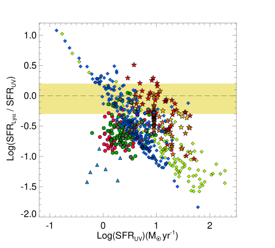
Figure 12: SFR(Ly$\alpha$) to SFR(UV) ratio as a function of SFR(UV). The color-code for the local sample is the same as previous figures. Several high-z samples are also included: green and blue diamonds (Gronwall et al. 2007; Guaita et al. 2010); yellow, orange and red stars (Curtis-Lake et al. 2012; Taniguchi et al. 2005; Jiang et al. 2013). The SFRs are observed values, not corrected for dust extinction.

The dashed line corresponds to the SFR ratio of unity. The yellow region denotes the SFR ratio values that would be derived for different star formation histories (see text for details).

7 Conclusion

We have analyzed a large sample Ly$\alpha$ emitters at redshift $z\sim 0$ and $z\sim 0.3$. We combined our spectroscopic follow-up of $z\sim 0.3$ galaxies, originally detected by Deharveng et al. (2008) with GALEX, with various data obtained from the literature to investigate the influence of several physical parameters on the escape of Ly$\alpha$ emission. After estimating the AGN contamination, we measured the oxygen abundance and the gas-phase extinction, using optical emission line ratios. We also derived the Ly$\alpha$ escape fraction, $f_{esc}$(Ly$\alpha$), using the H$\alpha$ flux and the nebular extinction. We summarize here the main conclusions we draw from the comparison of these parameters with the Ly$\alpha$ and UV properties.

• The Ly$\alpha$ escape fraction or equivalent width does not show a correlation with metallicity. While one may expect metal-poor galaxies to show strong Ly$\alpha$ emission as observed in Cowie et al. (2011), our results show that this is not always the case, and are in agreement with the observations of local blue compact galaxies, such as IZw 18 and SBS 0335.

• Looking at the Ly$\alpha$ equivalent width as a function of extinction, we do not find the trend commonly observed in high-redshift samples (e.g. Shapley et al. 2003; Pentericci et al. 2009). We explain the absence of correlation by the decoupling of the attenuation affecting the UV continuum and the multi-parameter process responsible for the attenuation the Ly$\alpha$ line. In addition, high-redshift studies use a model-dependent extinction that refers to the stellar extinction, which can be very different from the gas-phase dust encountered by Ly$\alpha$ photons.

• The Ly$\alpha$ escape fraction presents a clear correlation with the dust extinction, confirming earlier results (e.g. Atek et al. 2009a; Kornei et al. 2010; Hayes et al. 2011), albeit with a large dispersion indicating that dust attenuation is not the only regulatory factor of Ly$\alpha$ emission. A two-parameter fit of $f_{esc}$(Ly$\alpha$)-E(B-V) yields an extinction coefficient of $k_{Ly\alpha}\sim 6.67\pm 0.52$ and an intercept point of C${}_{Ly\alpha}=0.22\pm 0.03$. We see that even when no dust is present, the point of $f_{esc}$(Ly$\alpha$)=1 is only an upper limit and Ly$\alpha$ emission can be attenuated by the resonant scattering into neutral gas.

• We also introduce the normalized $f_{esc}$(Ly$\alpha$), which corresponds to the deviation of the observed $f_{esc}$(Ly$\alpha$) from what is expected from the case of pure dust attenuation. At low extinction, Ly$\alpha$ appears more attenuated than the UV continuum, most likely because of the scatting process. At higher extinction, $f_{esc}$(Ly$\alpha$) show above the predictions for standard dust attenuation. This can be the results of various mechanisms, including an enhancement of Ly$\alpha$ due to the ISM geometry (Neufeld 1991; Laursen et al. 2012; Verhamme et al. 2012), a different extinction law (Scarlata et al. 2009), a significant contribution from collisional excitation, or ionization by a hot plasma (Otí-Floranes et al. 2012).

• In order to assess the reliability of the Ly$\alpha$ emission line as a star formation indicator, we compared SFR(Ly$\alpha$) and SFR(UV), which has the advantage of being independent of the extinction. Overall, Ly$\alpha$ tend to underestimate the SFR by a factor up to 10. We observe that the SFR_Lyα/SFR_UV ratio is decreasing with increasing SFR_UV, which can be interpreted as a decrease in $f_{esc}$(Ly$\alpha$) as a function of UV luminosity as observed in several studies. We also note that this trend is being shifted with increasing redshift because of the redshift-dependence of the Ly$\alpha$ escape fraction.

Figure 13: Same as Fig. 1