A hot Jupiter transiting a mid-K dwarf found in the pre-OmegaCam Transit Survey

Abstract

We describe the pre-OmegaTranS project, a deep survey for transiting extra-solar planets in the Carina region of the Galactic disc. In 2006–2008, we observed a single dense stellar field with a very high cadence of $\sim$2 min using the European Southern Observatory Wide Field Imager at the La Silla Observatory.
Using the Astronomical Wide-field Imaging System for Europe environment and the Munich Difference Imaging Analysis pipeline, a module that has been developed for this project, we created the light curves of 16000 stars with more than 4000 data points which we searched for periodic transit signals using a box-fitting least-squares detection algorithm. All light curves are publicly available. In the course of the pre-OmegaTranS project, we identified two planet candidates – POTS-1b and POTS-C2b – which we present in this work.
With extensive follow-up observations we were able to confirm one of them, POTS-1b, a hot Jupiter transiting a mid-K dwarf. The planet has a mass of 2.31$\pm$0.77 M_Jup and a radius of 0.94$\pm$0.04 R_Jup and a period of $P$ = 3.16 d. The host star POTS-1 has a radius of 0.59$\pm$0.02 R_⊙ and a mass of 0.70$\pm$0.05 M_⊙. Due to its low apparent brightness of $I$ = 16.1 mag the follow-up and confirmation of POTS-1b was particularly challenging and costly.

1 Introduction

The field of transiting extra-solar planet detection has changed a lot in the last decade. After the first transit observations of the planet HD 209458b (Charbonneau et al., 2000) that had been detected using the radial velocity (RV) method, the OGLE-III deep survey (Udalski et al., 2004) was able to deliver the first detections of transiting planet candidates which were successfully confirmed with RV follow-up observations. The characteristics of this project allowed the detection of planets around faint stars which made any follow-up study difficult and expensive in terms of observing time. Nevertheless, the OGLE-III survey was the first to provide an estimate on the fraction of stars hosting a previously undetected population of very hot Jupiters with periods below 3 d (Fressin et al., 2007; Beatty & Gaudi, 2008). At the same time, several wide-angle surveys were initiated which target brighter stars using small-aperture optics such as TRES (O’Donovan et al., 2007), XO (McCullough et al., 2005), HAT (Bakos et al., 2004) and WASP (Pollacco et al., 2006). The number of known transiting planets was rising very quickly with each of them being an interesting target for follow-up studies such as the measurement of the spin–orbit alignment (e.g. Winn et al., 2009), thermal emission (e.g. Charbonneau et al., 2005), transit timing variations (e.g. Maciejewski et al., 2010; Fukui et al., 2011) or transmission spectroscopy studies (e.g. Berta et al., 2012).
The SWEEPS survey (Sahu et al., 2006) utilized the Hubble Space Telescope to search for short-period transiting planets in the Galactic bulge and found two planets and 14 additional candidates which are too faint ($V$ $>$ 19 mag) to be followed up and confirmed with current instrumentation. The launch of the CoRoT and Kepler satellites (Auvergne et al., 2009; Borucki et al., 2010) marked a new age of transit detection. An unprecedented precision of typically 10^-5 allows those missions to study the population of extra-solar planets down to Earth radii with great statistics. Up to now, 2312 planet candidates have been published by the Kepler team (Batalha et al., 2012) and even if the confirmation by RV measurements will be difficult and will take time, the expectation is that many of the detected objects are indeed planets (Morton & Johnson, 2011) although there are indications that the false positive rate varies significantly with planetary and stellar properties (Colón, Ford & Morehead, 2012).
Another comparably young branch of projects is formed by ground-based surveys dedicated to the detection of planets around M dwarfs. The MEarth project (Irwin et al., 2009) is monitoring bright M dwarfs with a network of small telescopes. The WFCAM Transit Survey (Kovács et al., 2013) is a deep J-band survey for planets around cool stars. M dwarfs have the advantage that their habitable zone is much closer compared to earlier spectral types making the detection of planets in this distance easier. Two large-area deep surveys, the Palomar Transient Factory (Law et al., 2011) and Pan-Planets (Koppenhoefer et al., 2009), are aiming at the detection of Jupiter- to Neptune-sized planets by observing of the order of 100000 M dwarfs.
In this work, we present the final results of the pre-OmegaTranS (POTS) project which is a pilot study for a larger scale transit survey that was planned to be conducted with the ESO Very Large Telescope (VLT) Survey Telescope (VST). In Section 2, we give an overview of the POTS including a description of the data reduction and light curve analysis. We present two planet candidates that we found in the survey. Section 3 summarizes several follow-up studies we conducted in order to confirm the planetary nature of our best candidate – POTS-1b. Using both photometric and spectroscopic observations, we were able to derive the mass and radius of the planet. Making use of high-resolution imaging with adaptive optics (AO) as well as a detailed analysis of the light curves enabled us to exclude all possible blend scenarios. In section 4, we present our second best candidate, POTS-C2 and in Section 5 we discuss the results and draw our conclusions.

2 The POTS Project

In 2004, a consortium of astronomers from INAF Capodimonte (Italy), Sterrewacht Leiden (Netherlands) and MPE Garching (Germany) designed the OmegaCam Transit Survey (OmegaTranS). A total of 26 nights of guaranteed time observations with OmegaCam (Kuijken et al., 2002) at the VST (Capaccioli, Mancini & Sedmak, 2002) were granted to this project by the three institutes. Scaling from existing surveys, such as OmegaTranS, was expected to deliver 10–15 new detections per year with the main power being the large 1 square degree field of view (FoV) of the OmegaCam detector.
Due to delays in the construction and commissioning of the telescope, the start of the project has been delayed and ultimately cancelled. Instead, we conducted the POTS using the ESO Wide Field Imager (WFI) mounted on the 2.2 m telescope at the La Silla observatory (Baade et al., 1999).
In Section 2.1, we present a characterization of the POTS target population. We obtained absolute magnitudes in the $U$, $B$, $V$, $R$ and $I$ filters and colours for each star in our target field. In Section 2.2, we give an overview of the POTS data collected in three observational seasons 2006–2008. The creation of the light curves using the difference imaging technique and the light-curve analysis and candidate selection are presented in Section 2.4.

2.1 Characterization of the POTS target population

In the course of the POTS, we observed one single WFI field (OTSF-1a) which is the north-west corner of the previously selected best OmegaTranS field OTSF-1 (Barbieri, 2007). The image centre is RA = 13^h35^m41$\aas@@fstack{s}$6 and Dec. = –$66^{\circ}$42’21” and the field dimensions are 34 arcmin $\times$ 33 arcmin.
In order to determine absolute magnitudes and colours for each star in our target field, we performed a photometric calibration. In 2006 March, we obtained observations of OTSF-1a in the $U$, $B$, $V$, $R$ and $I$ bands (filter #877, #878, #843, #844 and #879) as well as a set of standard star observations at several different airmasses.
We transformed the measured magnitude of each star into a calibrated magnitude in the Johnson–Cousins magnitude system using a filter-dependent extinction and a colour term. We assume the colour coefficients to be fixed properties of the WFI filters which are constant over time and therefore adapted the standard values obtained from the ESO/WFI instrument page. The extinction coefficients were measured using multiple observations of standard star fields (Landolt, 1992) which were taken at various airmasses (except for the $U$-band calibration where too few standard star field observations were available; we used the $U$-band extinction coefficient published on the WFI web page).
We performed aperture photometry on all standard stars using a large aperture with 30 pixel diameter ($\hat{=}$ 6 arcsec) which is much larger than the maximum full width at half maximum (FWHM) of the point spread functions (PSFs) of all images ($\sim$2 arcsec) and compared our measurements to a reference catalogue that has been exported from the Astronomical Wide-field Imaging System for Europe (Astro-WISE) (Valentijn et al., 2007) and which contains measurements from Landolt (1992), Stetson (2000) and from the Sloan Digital Sky Survey (SDSS) DR5 (Adelman-McCarthy et al., 2007). SDSS measurements were transformed into the Johnson–Cousins filter system using the equations given in Jester et al. (2005).
We assumed the extinction coefficient to be independent of CCD number and used the average of the values we obtained for the individual CCDs. Table 1 lists the measured extinction coefficients for the $B$, $V$, $R$ and $I$ bands as well as the extinction coefficient of the $U$ band and all colour coefficients that were taken from the WFI web page.
After the extinction and colour term correction, we derived a zero-point for each CCD and each filter by fitting a constant offset to the residuals. In order to check if we had to correct for zero-points variations over the FoV of one CCD (known as illumination correction), we analysed the residuals as a function of $x$- and $y$-position on the CCD and found no trends. We therefore used a constant zero-point for each CCD.
Table 2 lists our measured zero-points. The errors of the zero-points were estimated from the rms of the final residuals.

	$U$	$B$	$V$	$R$	$I$
Extinction coefficient	0.48	0.23	0.18	0.16	0.11
Colour coefficient	0.05	0.25	–0.13	0.00	0.03

Table 1: Extinction and colour coefficients used in this work.

CCD	$ZP_{U}$ (mag)	$ZP_{B}$ (mag)	$ZP_{V}$ (mag)	$ZP_{R}$ (mag)	$ZP_{I}$ (mag)
ccd50	22.32$\pm$0.06	24.77$\pm$0.03	24.12$\pm$0.04	24.46$\pm$0.05	23.36$\pm$0.09
ccd51	22.20$\pm$0.11	24.88$\pm$0.02	24.24$\pm$0.03	24.55$\pm$0.03	23.48$\pm$0.05
ccd52	22.20$\pm$0.09	24.66$\pm$0.04	24.01$\pm$0.03	24.37$\pm$0.06	23.29$\pm$0.07
ccd53	22.18$\pm$0.06	24.83$\pm$0.05	24.20$\pm$0.03	24.55$\pm$0.09	23.42$\pm$0.08
ccd54	22.24$\pm$0.12	24.80$\pm$0.03	24.15$\pm$0.04	24.54$\pm$0.09	23.41$\pm$0.08
ccd55	22.25$\pm$0.12	24.89$\pm$0.05	24.24$\pm$0.04	24.58$\pm$0.07	23.47$\pm$0.09
ccd56	22.14$\pm$0.10	24.82$\pm$0.04	24.19$\pm$0.04	24.51$\pm$0.05	23.39$\pm$0.05
ccd57	22.21$\pm$0.11	24.66$\pm$0.04	24.03$\pm$0.03	24.39$\pm$0.06	23.31$\pm$0.07

Table 2: Measured U-, B-, V-, R- and I-band zero-points for each CCD.

In order to derive the $U$-, $B$-, $V$-, $R$- and $I$-band magnitudes of all stars in our target field, we performed aperture photometry on each of the OTSF-1a images. Since the field is very crowded and our target stars are comparably faint, we used a small aperture of 15 pixels and applied an aperture correction to the measured fluxes. The aperture correction was determined by comparing the 15 and 30 pixel aperture fluxes of bright stars. For each filter, three observations of OTSF-1a were taken which gives us up to three independent measurements of each star. We use the median value for each star.
In a final step, we corrected our measurements for Galactic extinction. From Schlegel, Finkbeiner & Davis (1998), we obtained the total reddening for extragalactic objects $E(B-V)$ = 0.698. Assuming a standard extinction law, this translates in $E(U-B)$ = 0.64 $\times$ $E(B-V)$ = 0.45 (Binney & Merrifield, 1998). Since our target stars are located inside the Galaxy, the actual reddening should be lower than the extragalactic reddening (depending on the individual distance of each star). Fig. 1 shows the $UBV$ colour–colour plot of the OTSF-1a stars after correcting for an average reddening of half the extragalactic value (Schlegel, Finkbeiner & Davis, 1998). For individual sources (i.e. our detected transit candidates), we performed a more detailed analysis and derived individual extinction values and distances (see Section 2.4). Yellow and red lines indicate the location of main-sequence dwarfs and luminosity class III giants (according to Binney & Merrifield, 1998).

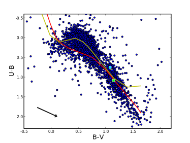
Figure 1: Extinction corrected $UBV$ colour–colour diagram of the 3000 brightest stars in the OTSF-1a field. The yellow and red lines show the position of the main-sequence and luminosity class III giants (according to Binney & Merrifield, 1998). The green and cyan squares show the positions of the planet POTS-1 and the candidate POTS-C2 which are presented in this work (see the text). The black arrow shows the extinction correction that has been applied.

2.2 Photometric observing campaigns 2006–2008

A total of 129 h of observations were collected in the years 2006–2008. Spread over 34 nights, we obtained 4433 epochs in the Johnson $R$ band (filter #844). The exposure time was 25 s in most cases. Under very good and very bad observing conditions, we slightly adjusted the exposure time in order to achieve a stable signal-to-noise ratio (S/N) or to avoid saturating too many stars. The average cadence (exposure, readout and file transfer time) is 107 s. The median seeing is 1.6 arcsec. 167 images with a seeing larger than 2.5 arcsec were not used because of their bad quality. Fig. 2 shows the probability to witness two or more transits as a function of the orbital period. The survey sensitivity drops quickly towards longer periods due to the limited amount of observing time that was available for this pilot study.
In addition to the science images, we obtained calibration images (i.e. bias and flat-field exposures) for each of the 34 nights.

Figure 2: Orbital phase coverage of the POTS light curves. The line shows the probability to see at least two transits for a given orbital period.

2.3 Data analysis and light-curve extraction

The basic CCD data reduction steps were done using the Astro-WISE standard calibration pipeline (Valentijn et al., 2007). The processing steps include overscan and bias correction, flat-fielding and masking of satellite tracks, bad pixels and cosmics. The data reduction pipeline treats all CCDs as independent detectors. For a complete description of all tasks, we refer to the Astro-WISE User and Developer manual.
All images of one CCD roughly map the same part of the sky. However, small shifts of the individual exposures (smaller than 20 pixels) arise from a limited pointing accuracy and a small dithering.
We calculated for each CCD the absolute astrometric solution for the very best seeing image by measuring the positions and brightnesses of several hundred stars with sextractor (Bertin & Arnouts, 1996) and comparing them to the positions in the USNO-A2.0 catalogue. Using least-squares methods, a transformation was calculated that corrects for a shift, a rotation and a third-order polynomial distortion.
We combined the 15 best seeing images of each CCD (typically around 0.6 arcsec FWHM) to create a reference stack which was then used to perform a relative astrometric calibration of all single images. In this way, we achieved a median rms of the astrometric solutions of 40 mas. Note that a very good overlap is important for the difference imaging approach (see below). Out of the 4266 single images, 12 had an rms of the astrometric residuals that was larger than 0.1 arcsec and were not used in the following steps. Each image was resampled to a new grid with a pixel scale of 0.2 arcsec pixel^-1 using the program swarp which uses a LANCZOS3 interpolation algorithm.
We applied the Munich Difference Imaging Analysis (mdia) package (Koppenhoefer, Saglia & Riffeser, 2013) to the resampled images in order to create light curves using the difference imaging method (Tomaney & Crotts, 1996; Alard & Lupton, 1998). The technique has become the most successful method used for the creation of high-precision light curves in crowded fields such as the Milky Way bulge (Udalski et al., 2008) or the Andromeda Galaxy (Riffeser, Seitz & Bender, 2008). The mdia package is based on the implementation presented in Gössl & Riffeser (2002).
The method uses a reference image which is degraded by convolution in order to match the seeing of each single image in the data set. Subtracting the convolved reference image from a single image, one gets a so-called difference image with all constant sources being removed and variable sources appearing as positive or negative PSF-shaped residuals.
In the difference imaging process, we adopted the standard parametrization of the kernel base functions (Alard & Lupton, 1998) and a kernel size of 41 $\times$ 41 pixels, together with a third-order polynomial to account for background differences. The 60 free parameters were determined via $\chi^{2}$-minimization. We used almost all pixels to determine the optimal kernel and background coefficients. Only pixels that belong to variable objects were not taken into account since these would have destroyed the normalization of the kernel. As we did not know a priori which pixel belong to variable objects, we first created a subset of difference images without masking any pixel, identified variable objects and masked them in the second run when we created all difference images. In order to account for small variations of the PSF over the FoV of the detector, we split each image into 4 $\times$ 8 subfields and determine a kernel in each of the subfields independently.
To construct the light curves of each object, we combine the differential fluxes measured in the difference images with the constant flux measured in the reference image. The flux measurements in the reference image were done with usmphot which is an iterative PSF-fitting program that is very similar to daophot (Stetson, 1987).
The photometry on the difference image was done also with PSF photometry. We constructed the PSF from the normalized convolved reference image using the same isolated stars we used to measure the fluxes in the reference image. Note that in this way we automatically obtained the differential fluxes in the same units as in the reference image which results in correct amplitudes (i.e. transit depths).
In a final step, we normalized the fluxes of all light curves to 1 (i.e. divided by the median flux) and applied a barycentric time correction using the formulae of Meeus (1982) as implemented in the skycalc program by Thorstensen.

2.4 Light-curve analysis and candidate selection

For each CCD, we extracted the light curves of the 2000 brightest sources. Fig. 3 shows the magnitude distribution of the selected objects. In order to correct for red noise, we applied the $sysrem$ algorithm (Tamuz, Mazeh & Zucker, 2005) which has turned out to be very successful in reducing systematic effects and which is used in a large number of transit surveys (e.g. Pont, Zucker & Queloz, 2006; Snellen et al., 2007).
$Sysrem$ works most efficiently if all light curves of variable stars are removed from the sample. Therefore, we fitted a constant baseline to each light curve and calculated the reduced $\chi^{2}$ of the fit. We applied the $sysrem$ algorithm to all light curves with $\chi^{2}$ $\leq$ 1.5 (70 per cent of all light curves) and subtracted four systematic effects.
Fig. 4 shows the rms of the light curves before (black points) and after the $sysrem$ correction (red points). The black line shows the theoretical rms for 25 s exposure time, airmass 1.4, sky brightness of 20.3 mag arcsec^-2 and 1.5 arcsec seeing and 0.0005 mag scintillation noise [estimated using the formula of Young (1967)]. The other lines show the contributions of the different noise components. Note that the magnitude-independent scintillation noise is outside the limits of the figure. The $sysrem$ algorithm reduced the rms of the light curves by only a small amount. We therefore conclude that systematic effects in our data set are not as prominent as is the case for other surveys (see e.g. Pont, Zucker & Queloz, 2006; Snellen et al., 2007). At the bright end, we reached a photometric precision of $\sim$2–3 mmag which is close to the theoretical precision.

Figure 3: Magnitude histogram of all selected sources in the POTS.

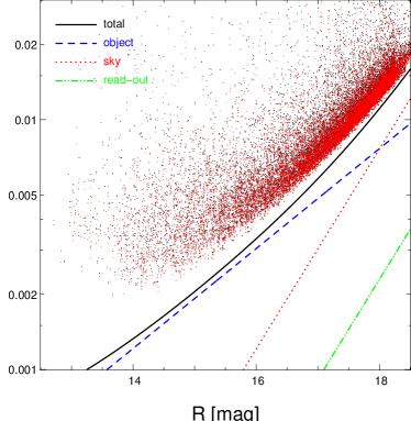
Figure 4: rms before (black points) and after (red points) application of the $sysrem$ algorithm. The black line shows the theoretical rms for our survey parameters. The blue dashed and the red dotted lines show the contribution of the photon noise from object and sky background, respectively, and the green dash–dotted line shows the contribution of the readout noise.

In order to find transiting planet candidates, we applied the box-fitting least-squares (BLS) algorithm proposed by Kovács, Zucker & Mazeh (2002) to all $sysrem$-corrected light curves. We tested 4001 different periods equally spaced in 1/$p$ between 0.9 and 9.1 d. We used 1000 bins in the folded light curves. Note that the choice of only 4001 different periods could be questioned since the survey data span a period of 572 d which would correspond to 63 or 636 revolutions for the longest and shortest periods, respectively. In the worst case (i.e. when the true period is exactly between two tested periods), the uncertainty adds up to a phase shift between the first and the last observations of 0.07 or 0.04 phase units, respectively. This is of the same order of the typical fractional transit duration (0.01 and 0.1 phase units for the longest and shortest periods) and our choice of 4001 test periods in principle could have limited our survey sensitivity. However, 95 per cent of the data were taken within a period of 241 d (2006 July to 2007 May) and therefore the impact on the survey sensitivity is not very strong.
We determined the survey sensitivity using Monte Carlo simulations (Koppenhoefer, 2009). The overall efficiency of 23 per cent was relatively low mainly due to the limited amount of total observing time.
For each light curve we determined the best-fitting period $P$, epoch $t_{0}$, transit depth $\Delta F$/$F$ and fractional transit length $\tau$. We also determine the number of transits, number of data points during a transit, the S/N of the light curve and the SDE of each detection and calculate the reduced $\chi^{2}$ of the box fit.
As an additional very useful parameter, we measured the variations that are in the out-of-transit part of the light curve. After masking the detected signal, we run the BLS algorithm again on the remaining data points and compare the S/N found in the masked light curve, S/N${}_{\textrm{removed}}$ hereafter, to the S/N found in the unmasked light curve. In the case of variable stars, the difference between the two values (S/N - S/N${}_{\textrm{removed}}$) is expected to be low, whereas for a transiting planet the difference should be high.
In order to identify all interesting transiting planet candidates and to reject variable stars and other false positives, we applied three selection criteria: we require a minimum of two transits (otherwise the period of the orbit could not be determined). Furthermore, we require S/N $\geq$ 12 and (S/N - S/N${}_{\textrm{removed}}$) $\geq$ 4.7. The last two selection criteria were optimized using Monte Carlo simulations. More details about the optimization procedure can be found in Koppenhoefer (2009).

Among $\sim$200 light curves that passed the detection criteria presented in the previous section, we identified two transiting planet candidates. The remaining detections were visually classified as variable stars or false detections caused by systematic outliers. Due to limited observing time in combination with the faintness of the candidates we decided to follow up only the best candidate, i.e. POTS-1. The quality of the candidate POTS-C2 is also good; however, we decided to concentrate on POTS-1 because it is brighter (0.8 mag in $I$) and slightly redder.
We present our intensive spectroscopic and photometric follow-up observations of POTS-1 in Section 3 which lead to a confirmation of the planetary nature of POTS-1b. In Section 4, we present the candidate POTS-C2 which we propose for follow-up in the future. Fig. 5 shows a 1.5 $\times$ 1.5 arcmin finding chart for each of the two objects.

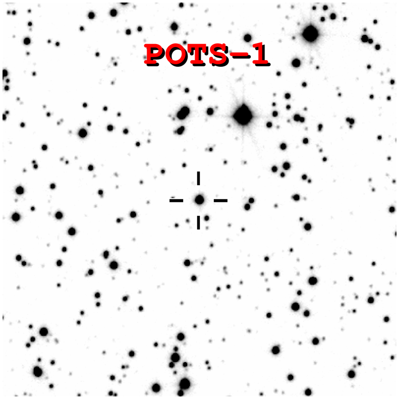
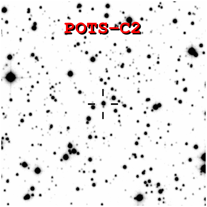
Figure 5: Finding chart of POTS-1 and POTS-C2. The FoV is 1.5 $\times$ 1.5 arcmin. North is up and east is left.

3 Follow-up and confirmation of POTS-1

In the last years we performed several complementary follow up studies which allowed us to confirm one of our candidates, POTS-1b, as a planet. In section Section 3.1, we describe the spectroscopic observations we used to determine the atmospheric parameters of the host star as well as the mass of POTS-1b. In Section 3.2, we present the combined analysis of the POTS light curve together with targeted multiband observations of three additional transits. With high angular resolution adaptive imaging we excluded contaminating sources in the vicinity of POTS-1, as described in Section 3.3. Finally, in Section 3.4 we describe how we ruled out possible blend scenarios.

3.1 Spectroscopic observations with UVES

3.1.1 Observations and reduction of the spectra

We observed POTS-1 with the UV–Visual Echelle Spectrograph (UVES; Dekker et al., 2000), mounted at the Nasmyth B focus of UT2 of ESO’s VLT at Paranal, Chile. The aim of these observations was to estimate the spectroscopic parameters of the host star, and to determine the RV variations which then allowed us to estimate the mass of the transiting object.
In 2009, we collected a total of 10 observations in fibre mode, with UVES connected to the FLAMES facility (Pasquini et al., 2002). We used a setup with a central wavelength of 580 nm, resulting in a wavelength coverage of 4785–6817$\AA$ over two CCDs, at a resolving power of R = 47000. Due to the faintness of the target, we had to use long exposure times of 46 min. Three observations turned out to have a high background contamination due to stray light within the detector. We were not able to use those data but we got compensation in the form of a re-execution in 2010.
In 2010, we collected seven observations with UVES in slit mode. The exposure times were 48 min. We chose a slit width of 1 arcsec which translates into a resolving power of R = 40000. We used the standard setup with a central wavelength of 520 nm, resulting in a wavelength coverage of 4144$-$6214$\AA$.
Both UVES data sets were reduced using the midas-based pipelines provided by ESO, which result in fully reduced, wavelength-calibrated spectra. Unfortunately, the pipeline for fibre-mode observations failed to extract the spectra of four of our observations.
Table 3 gives an overview of the spectroscopic observations that are used in this work. The S/N per resolution element, in the central part of the red orders, varied between 10 and 30 for the different epochs.

3.1.2 Spectroscopic analysis of the host star

We estimated the atmospheric parameters and chemical abundances of POTS-1 analysing simultaneously the spectral energy distribution (SED) and high-resolution spectra obtained combining the seven epochs taken in slit mode. The combined spectrum has an S/N of 43.4 per resolution element in the central parts of the spectral region.
For both SED and spectral analysis we employed the marcs stellar model atmosphere code from Gustafsson et al. (2008). For all calculations, local thermodynamical equilibrium and plane-parallel geometry were assumed, and we used the vald data base (Piskunov et al., 1995; Kupka et al., 1999; Ryabchikova et al., 1999) as a source of atomic line parameters for opacity calculations and abundance determination.
We first derived the effective temperature $T_{\mathrm{eff}}$ by imposing simultaneously the Ti i excitation equilibrium and the Ti ionization equilibrium and by fitting synthetic fluxes to the available photometry (see Section 3.1.3). We adopted Ti because it is the only atom for which we measured a significant number of lines, with reliable $\log gf$ values, of two ionization stages. In addition, the measured Ti i lines have a much more uniform distribution in excitation energy, compared to any other measured ion. We derived the line abundance from equivalent widths analysed with a modified version (Tsymbal, 1996) of the width9 code (Kurucz, 1993).
We determined $T_{\mathrm{eff}}$ assuming first a $\log g$ value of 4.7 (typical of a main-sequence mid-K-type star) and a microturbulence velocity ($\upsilon_{\mathrm{mic}}$) of 0.85 km s^-1 (Valenti & Fischer, 2005). We could make this first assumption because in this temperature regime both equilibria (excitation and ionization) and the SED are almost completely insensitive to $\log g$ and $\upsilon_{\mathrm{mic}}$ variations (Morel, & Miglio, 2012). We finally obtained and adopted an effective temperature of 4400$\pm$200 K.
Having fixed $T_{\mathrm{eff}}$, and knowing that $\log g$ variations have negligible effects on $\upsilon_{\mathrm{mic}}$ determination, we measured the microturbulence velocity by imposing the equilibrium between the line abundance and equivalent widths for Tii, obtaining 0.8$\pm$0.3 $\mathrm{km\,s}^{-1}$, in agreement with what is commonly measured for late-type stars (Pavlenko et al., 2012).
In order to derive the metallicity of POTS-1, we measured a total of 54 Fe i lines from which we obtained an average abundance, relative to the Sun (Asplund et al., 2009) of $[$Fe/H$]$ = $-$0.03$\pm$0.15, where the uncertainty takes into account the uncertainties on the atmospheric parameters (see Fossati et al. (2009) for more details). We measured also the abundance of Mg, Al, Si, Ca, Sc, Ti, V, Cr, Mn, Co, Ni, Y, Zr and Ba, all of them being consistent with the solar values. The fit of synthetic spectra to the observed spectrum did not require the addition of any rotational broadening; therefore, the stellar projected rotational velocity (${\upsilon}\sin i$) is constrained by the minimum measurable ${\upsilon}\sin i$ allowed by the resolution of the spectrograph. With the given spectral resolution of 40000, ${\upsilon}\sin i$ is $\leq$ 5.3 $\mathrm{km\,s}^{-1}$, in agreement with the derived evolutionary status of the star.
In a completely independent analysis of the spectroscopic data, we fitted synthetic models computed by the wita6 program (Pavlenko, 1997) for a grid of sam12 model atmospheres (Pavlenko, 2003) of different $T_{\mathrm{eff}}$, $\log g$, $[$Fe/H$]$ and find stellar parameters which are in very good agreement with the ones derived with the marcs models.
Figs 6 and 7 show the Dartmouth isochrones in the range from 1 to 13 Gyr for solar metallicity (Dotter et al., 2008). The $\log g$ and mass evolution of a mid-K dwarf over the age of the Universe is rather small. Given the possible range for $T_{\mathrm{eff}}$ , we constrain the surface gravity to $\log g$  = 4.63$\pm$0.05 and the mass to M_⋆ = 0.695$\pm$0.050 M_⊙. We compared these results to the values obtained using low-mass stellar evolution models from Baraffe et al. (1998) which agree very well ($\log g$  = 4.66$\pm$0.04 and M_⋆ = 0.70$\pm$0.06 M_⊙).
As a spectroscopic confirmation of the derived $\log g$ value, Fig. 8 shows a region of the summed spectra centred on the Na i D lines together with synthetic spectra of three different surface gravities which underlines our adopted value of $\log g$  = 4.63.

BJD	Mode	Phase	S/N	RV	Bisector span
2454924.70252	Fibre	0.278	12.2	–16.779$\pm$0.358 km s-1	0.112$\pm$0.382 km s-1
2454924.73647	Fibre	0.288	12.9	–16.879$\pm$0.378 km s-1	–0.001$\pm$0.229 km s-1
2454924.77903	Fibre	0.302	16.3	–16.739$\pm$0.428 km s-1	0.024$\pm$0.197 km s-1
2454924.81228	Fibre	0.313	16.2	–16.476$\pm$0.578 km s-1	–0.128$\pm$0.228 km s-1
2455066.49230	Fibre	0.139	12.6	–17.252$\pm$0.532 km s-1	–0.060$\pm$0.227 km s-1
2455258.62018	Fibre	0.928	20.1	–16.289$\pm$0.552 km s-1	0.304$\pm$0.209 km s-1
2455289.79078	Slit	0.790	14.8	–15.976$\pm$0.401 km s-1	0.000$\pm$0.152 km s-1
2455327.63875	Slit	0.765	15.6	–15.871$\pm$0.329 km s-1	0.117$\pm$0.143 km s-1
2455349.61383	Slit	0.718	12.5	–15.629$\pm$0.569 km s-1	–0.326$\pm$0.180 km s-1
2455376.49998	Slit	0.224	11.9	–15.941$\pm$0.354 km s-1	–0.156$\pm$0.163 km s-1
2455384.53550	Slit	0.767	16.4	–15.512$\pm$0.514 km s-1	0.259$\pm$0.196 km s-1
2455387.52652	Slit	0.713	14.3	–15.947$\pm$0.308 km s-1	–0.031$\pm$0.192 km s-1
2455387.56369	Slit	0.725	13.2	–15.701$\pm$0.304 km s-1	0.058$\pm$0.161 km s-1

Table 3: Overview of the spectroscopic observations of POTS-1 taken with UVES. The first four columns give the Barycentric Julian Date of the exposure mid-point, the instrument mode, the planet’s orbital phase at the time of observation and the average signal-to-noise ratio of the spectra per resolution element. Columns 5 and 6 give the RV and the bisector span measurements.

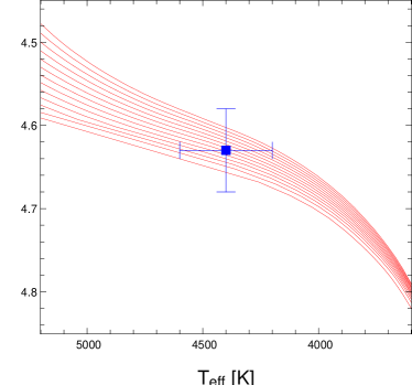
Figure 6: log $g$ – $T_{\mathrm{eff}}$ relation for low-mass stars showing isochrones of 1 to 13 Gyr for solar metallicity (Dotter et al., 2008). Assuming that POTS-1 is on the main sequence, we derive a $\log g$ of 4.63$\pm$0.05 using the estimate for $T_{\mathrm{eff}}$ derived from SED fitting.

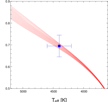
Figure 7: Mass – $T_{\mathrm{eff}}$ relation for low-mass stars. The lines show isochrones ranging from 1 to 13 Gyr for solar metallicity (Dotter et al., 2008). Assuming that POTS-1 is on the main sequence, we derive a mass of 0.695$\pm$0.050 M_⊙ using the estimate for $T_{\mathrm{eff}}$ derived from SED fitting.

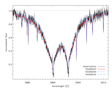
Figure 8: Comparison between the observed Na i D lines (black solid line) and synthetic profiles calculated with our final adopted parameters (red thick line) and with $\log g$ increased by 0.3 dex (blue dashed line) and decreased by 0.3 dex (blue dash–dotted line). Interstellar absorption is visible just redwards of the cores of the Na i D lines.

$T_{\mathrm{eff}}$	=	4400$\pm$200 K
$\log g$	=	4.63$\pm$0.05
$[$Fe/H$]$	=	–0.03$\pm$0.15
$\upsilon_{\mathrm{mic}}$	=	0.8$\pm$0.2 $\mathrm{km\,s}^{-1}$
${\upsilon}\sin i$	$\leq$	5.3 $\mathrm{km\,s}^{-1}$
$M_{s}$	=	0.695$\pm$0.050 M⊙
$K$	=	407$\pm$117 m s-1
$M_{p}$	=	2.31$\pm$0.77 MJup

Table 4: Stellar parameters of POTS-1 and RV amplitude as determined from our spectroscopic observations and SED fitting.

3.1.3 Spectral energy distribution

We extracted the $UBVRI$ magnitudes of POTS-1 from the photometric calibration (see Section 2.1). In addition, we cross-matched with the 2MASS All-Sky Point Source Catalog (PSC) (Skrutskie et al., 2006) and identified POTS-1 as object 13342613–6634520 and extracted the $JHK$ magnitudes. All magnitudes are listed in Table 5.
Using the optical and NIR photometry, we derived $T_{\mathrm{eff}}$ making use of the marcs synthetic fluxes (Gustafsson et al., 2008). Without accounting for any reddening, it was not possible to fit POTS-1’s SED assuming any $T_{\mathrm{eff}}$, when using simultaneously both the WFI and 2MASS photometry. By adding the reddening to the SED, we derived a best-fitting temperature of $T_{\mathrm{eff}}$ = 4400$\pm$200 K and reddening of $E(B-V)$ = 0.40$\pm$0.05 mag, where the optical photometry provided the strongest constraint to the reddening while the NIR photometry constrained mostly $T_{\mathrm{eff}}$. Fig. 9 shows our best fit. It is important to mention that at these temperatures, the SED is only very little dependent on the other atmospheric parameters of the star, such as $\log g$ or metallicity. Our best-fitting reddening value is in good agreement with that obtained from galactic interstellar extinction maps by Amôres & Lépine (2005).
Given the reddening and the galactic coordinates of the star, we derived a distance to the star of 1.2$\pm$0.6 kpc. To independently check our results, we calculated the distance to the star from the $V$ magnitude (corrected for the reddening), the effective temperature (4400 K) and a typical main-sequence radius of 0.67 R_⊙, obtaining a distance of about 0.9 kpc, in agreement with what was previously derived.

POTS-1 (2MASS 13342613–6634520)
RA (J2000.0)	13h34m26$\aas@@fstack{s}$1
Dec. (J2000.0)	–66∘34′52′′
$U$	20.89$\pm$0.10 mag
$B$	19.54$\pm$0.04 mag
$V$	17.94$\pm$0.03 mag
$R$	17.01$\pm$0.06 mag
$I$	16.14$\pm$0.07 mag
$J$	15.17$\pm$0.06 mag
$H$	14.38$\pm$0.04 mag
$K$	14.24$\pm$0.08 mag
$d$	1.2$\pm$0.6 kpc
$E(B-V)$	0.40$\pm$0.05 mag
$T_{\mathrm{eff}}$	4400$\pm$200 K
Spectral type	K5V

Table 5: Basic parameters of the POTS-1 system.

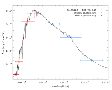
Figure 9: SED fitting for POTS-1. The plot shows the comparison between marcs model theoretical fluxes calculated with $T_{\mathrm{eff}}$ = 4400 K and log $g$ = 4.7 (our final set of fundamental parameters), taking into account a reddening of E($B$-$V$) = 0.40 mag, with the Johnson–Cousins $UBVRI$ photometry (red crosses) and 2MASS photometry (blue asterisks).

To confirm that POTS-1 hosts a planet, it is crucial to completely exclude that it is a giant. The sole constraint given by the Na i D line profile is not enough to guarantee that the star is not a giant, as these lines could be fitted by various sets of $T_{\mathrm{eff}}$ and $\log g$, i.e. lower gravity and lower temperature such as $T_{\mathrm{eff}}$ = 3950 K and log $g$ = 3.0. However, to fit the SED with such a set of stellar parameters, we would require a reddening much smaller than 0.40 mag. If we now assume that the star is a giant, because of the large radius, the star would be at a distance much larger than 1.2 kpc, implying a reddening much larger than 0.40 mag, in contradiction with what was required to fit the SED. Note that a large radius of POTS-1 can also be excluded from the mean stellar density obtained in the light-curve fitting (see below).
Table 4 lists all host parameters that we derived from the combined analysis of the spectroscopic data and SED fitting.

3.1.4 RV analysis

To calculate the RV variations of POTS-1 caused by the transiting object, we cross-correlated the orders of the 13 spectra with a Kurucz synthetic model spectrum for a star with $T_{\mathrm{eff}}$ = 4500 K and $\log g$  = 4.5 (the model grid has a resolution of 250 K and 0.5 dex). The resulting barycentric corrected RV measurements are presented in Table 3. The uncertainties have been estimated from the variation of the RV estimates obtained for the different echelle orders. The final RV measurements as a function of orbital phase are shown in Fig. 10. We fitted the data with a sine function with amplitude and zero-point velocity as free parameters. We find a best-fitting RV amplitude of K = 407$\pm$117 m s^-1, with V₀ = –16.234 km s^-1. Using the period obtained from the transit fit, the RV curve fit and the stellar parameters derived above, we obtain a planetary mass of M_p = 2.31$\pm$0.77 M_Jup.
In order to check for line asymmetries, we determined the values of the bisector span (following Queloz et al., 2001) as a function of orbital phase which are shown in Fig. 11. A least-squares fit of the bisector span measurements with a sine function revealed no significant variations at a level of 0.045$\pm$0.056 km s^-1. Although this means that there is no indication that the measured RV variations are due to line-shape variations, caused by either stellar activity or blends, the errors are very large, making any claim based on the bisector span uncertain.
Due to the specific scheduling of the observations, most of the measurements around phase $\sim$0.25 are taken in 2009 and most of the observations around phase $\sim$0.75 in 2010. As a consequence, the variation of the RV of POTS-1 can also be explained by a linear trend which could be caused by a long-period massive companion to POTS-1. Fig. 12 shows the distribution of the RV measurements in time together with the best-fitting linear trend. Although there is no indication that a long-period companion to POTS-1 exists, we explore this scenario by removing the linear trend and fitting a sinusoidal RV variation to the residuals. The resulting semi-amplitude is K = 35${}^{+151}_{-35}$ m s^-1 which corresponds to a planetary mass of M_p = 0.20${}^{+0.67}_{-0.20}$ M_Jup.
Alternatively, the detected RV variation can be explained by an offset between the UVES slit-mode and fibre-mode measurements. RV offsets of up to a few 100 m s^-1 are commonly found when combining RV observations from different instruments (see e.g. Pasquini et al., 2012). The solid red and blue lines in Fig. 12 show the average of all measurements taken with UVES in slit mode and fibre mode, respectively. Fitting a sinusoid to the RV measurements of the observations taken in different modes independently we find a semi-amplitude of K = 337${}^{+203}_{-202}$ m s^-1 for the fibre-mode obesrvations and a semi-amplitude of K = 67${}^{+142}_{-67}$ m s^-1 for the slit-mode observations which translates into mass estimates of M_p = 1.91${}^{+1.30}_{-1.19}$ and 0.38${}^{+0.86}_{-0.38}$ M_Jup, respectively.

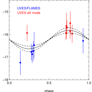
Figure 10: The RV measurements of POTS-1 as a function of orbital phase. The solid and dashed lines show the best-fitting velocity amplitude and 1$\sigma$ upper and lower limits of the determined RV amplitude.

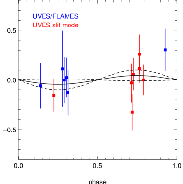
Figure 11: Bisector variations as a function of orbital phase. The solid line and dashed lines in the top panel indicate the least-squares fit to the sinusoidal variation in the bisector span and its uncertainty at 0.004$\pm$0.012 km s^-1.

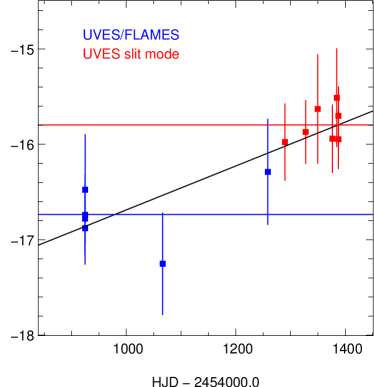
Figure 12: The RV measurements of POTS-1 as a function of BJD. A linear trend which could be caused by an undetected stellar companion fits the data quite well. In this case, the 1$\sigma$ upper limit for the mass of the planet would be 0.87 M_Jup as measured by a least-squares fit to the residuals.

3.2 Photometric transit observations with GROND

In order to precisely determine the physical parameters of the POTS-1 system such as period, $t_{0}$, planet radius and orbital inclination, we observed three full transits of POTS-1 with the GROND instrument (Greiner et al., 2008) mounted on the MPI/ESO 2.2m telescope at the La Silla observatory. The GROND instrument has been used several times for the confirmation of a transiting planet candidate (e.g. Snellen et al., 2009) and for detailed follow-up studies of known transiting extra-solar planets (see e.g. Lendl et al., 2010; de Mooij et al., 2012; Nikolov et al., 2012). GROND is a seven-channel imager that allows us to take four optical ($g^{\prime}$, $r^{\prime}$, $i^{\prime}$ and $z^{\prime}$) and three near-infrared ($JHK$) exposures simultaneously. For our observations, the $JHK$ light curves turned out to have a large scatter; we therefore did not use them in our analysis.
We observed POTS-1 during the nights of 2009 April 17, 2010 April 6 and 2010 July 13 and collected a total of 84, 68 and 123 images in each optical band. The exposure time was ranging from 133 to 160 s resulting in a cycle rate of about 3.5 min.
All optical images were reduced with the mupipe software developed at the University Observatory in Munich. After the initial bias and flat-field corrections, cosmic rays and bad pixels were masked and the images were resampled to a common grid. The frames did not suffer from detectable fringing, even in the z’ band. We performed aperture photometry on POTS-1 and typically 10 interactively selected reference stars after which light curves were created for each of the four bands.
In order to account for the wide range of seeing conditions, the aperture radii were chosen between 4 and 16 pixels (corresponding to 0.6–2.4 arcsec) by minimizing the rms scatter in the out of transit part of the light curves. For each band at a given night, we used a fixed aperture size. The sky background was determined as the median value in an annulus with an inner radius of 25 and an outer radius of 30 pixels measured from the object centre positions.
The light curves were fitted with analytic models presented by Mandel & Agol (2002). We used quadratic limb-darkening coefficients taken from Claret & Bloemen (2011), for a star with metallicity $[\rm{Fe/H}]$ = 0.0, surface gravity log $g$ = 4.7 and effective temperature $T_{\mathrm{eff}}$ = 4400 K. The values of the limb-darkening coefficients are obtained as linear interpolations of the available grid.
Using a simultaneous fit to the individual light curves in all five bands (the four optical GROND bands plus the WFI R band) we derived the period $P$, epoch $t_{0}$, mean stellar density $\rho_{s}$ = $M_{s}$ / $R^{3}_{s}$ in solar units, the radius ratio $R_{p}$ / $R_{s}$ and the impact parameter $\beta_{\rm{impact}}$ (in units of $R_{s}$). Together with three scaling factors for each GROND filter (one for each night) and one scaling factor for the R-band light curve, a total of 18 free parameters were fitted. The light curves and the best-fitting models are shown in Figs. 13–17. The rms values of the residuals in the combined light curves are 8.9, 3.6, 3.8, 5.4 and 7.7 mmag for $g^{\prime}$, $r^{\prime}$, $i^{\prime}$, $z^{\prime}$ and R bands, respectively.
Using the stellar mass estimate of $M_{s}$ = 0.695$\pm$0.050 M_⊙ as derived in Section 3.1, we calculate the radius of the star and the planet, as well as the inclination of the orbit. In order to derive uncertainties of the system parameters, we minimized the $\chi^{2}$ on a grid centred on the previously found best-fitting parameters and searched for extreme grid points with $\Delta\chi^{2}$ = 1 when varying one parameter while simultaneously minimizing over the others. The resulting final parameters and error estimates are listed in Table 6. Note that the best-fitting value of $\log g$ based on the light curves is in reasonable agreement with the value derived from the spectra and colours.
We fit the individual transits in order to search the light curves for transit timing variations. The WFI R-band light curve shows only a single complete transit. Together with the three transits observed with GROND, we find the central transit times reported in Table 7. We find no significant transit timing variations.

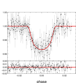
Figure 13: Folded $g^{\prime}$-band light curve of POTS-1 containing the observations of three individual transits. The red line shows the best-fitting model with the parameters listed in Table 6.

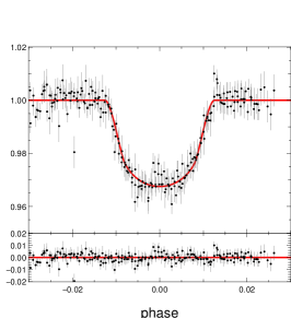
Figure 14: Folded $r$’-band light curve of POTS-1 containing the observations of three individual transits. The red line shows the best-fitting model with the parameters listed in Table 6.

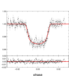
Figure 15: Folded $i^{\prime}$-band light curve of POTS-1 containing the observations of three individual transits. The red line shows the best-fitting model with the parameters listed in Table 6.

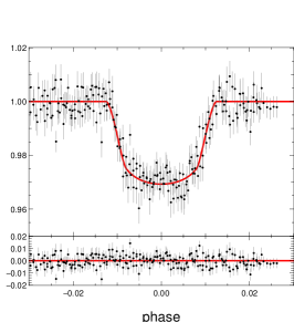
Figure 16: Folded $z^{\prime}$-band light curve of POTS-1 containing the observations of three individual transits. The red line shows the best-fitting model with the parameters listed in Table 6.

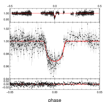
Figure 17: Folded POTS R-band light curve of POTS-1. The red line shows the best-fitting model with the parameters listed in Table 6. Note that due to a deficiency of points at phase 0.5, the R-band light curve would be consistent with a period that is actually half the detected period (i.e. with each second eclipse being hidden in the gap). However, we ruled this out with additional GROND observations at phase 0.5 which showed no sign of the eclipse.

$\rho_{s}$	=	3.417${}^{+0.410}_{-0.261}$ $\rho_{\rm{\odot}}$
$R_{p}$ / $R_{s}$	=	0.16432${}^{+0.00176}_{-0.00218}$
$\beta_{\rm{impact}}$	=	0.459${}^{+0.045}_{-0.073}$
$t_{0}$	=	2454231.65488$\pm$4.4$\times 10^{-4}$ BJD
$P$	=	3.16062960$\pm$1.57$\times 10^{-6}$ d
$i$	=	88$\aas@@fstack{\circ}$06${}^{+0.47}_{-0.34}$
$R_{p}$	=	0.941${}^{+0.036}_{-0.047}$ RJup
$R_{s}$	=	0.588${}^{+0.020}_{-0.028}$ R⊙
$\log g$	=	4.74$\pm$0.07
$a_{p}$	=	0.03734$\pm$0.00090 AU

Table 6: The orbital, host star and planetary parameters of the POTS-1 system as determined from the photometric observations.

Civil date	Filter	$t_{0}$ (BJD)	O–C
14.03.2007	$R$	2454174.76322$\pm$7.0$\times 10^{-4}$	–3.3$\times 10^{-4}$
17.04.2009	$griz$	2454939.63572$\pm$2.9$\times 10^{-4}$	–1.9$\times 10^{-4}$
06.04.2010	$griz$	2455293.62673$\pm$3.8$\times 10^{-4}$	3.0$\times 10^{-4}$
13.07.2010	$griz$	2455391.60583$\pm$3.7$\times 10^{-4}$	–1.1$\times 10^{-4}$

Table 7: Central times $t_{0}$ for the individual transits observed with WFI and GROND. No significant transit timing variations are detected.

3.3 High-resolution imaging with NACO

On 2011 March 25 we obtained follow-up high-contrast imaging observations of POTS-1 with NACO (Lenzen et al., 2003; Rousset et al., 2003), the AO imager of ESO-VLT, at the Paranal observatory in Chile. The wavefront analysis was performed with NACO’s visible wavefront sensor VIS, using the AO reference star 2MASS J13342468–6634348 (V$\sim$15.1 mag, $K_{s}$$\sim$9.3 mag), which is located about 19.2 arcsec north-west of POTS-1.
The observations were carried out at an airmass of about 1.35 with a seeing of $\sim$0.8 arcsec and coherence time $\tau_{0}\sim$3 mas of the atmosphere in average, which corresponds to a value of the coherent energy of the PSF of the star of 33$\pm$4 per cent.
We took 21 frames with NACO’s high-resolution objective S13 (pixel scale 13.23 mas pixel^-1 and 13.5 arcsec $\times$ 13.5 arcsec FoV) in the $K_{s}$ band each with a detector integration time of 60 s, in the HighDynamic detector mode. For the subtraction of the bright background of the night sky in the $K_{s}$ band, the telescope was moved between individual integrations (standard jitter mode) with a jitter width of 7 arcsec, sufficiently large to avoid overlapping of the PSF of detected sources.
For the flat-field correction, internal lamp flats as well as skyflats were taken before and after the observations during daytime or twilight, respectively. The data reduction (background estimation, background subtraction, and then flat-fielding), as well as the final combination (shift+add) of all images, was then performed with eso-eclipse (Devillard, 2001).
Our fully reduced NACO image of POTS-1 is shown in Fig. 18. The elliptical shape of the PSF is due to the fact that we observed the object outside the isoplanatic angle. This was necessary because POTS-1 is too faint to be used as AO reference and we had to choose a brighter nearby reference. A careful look at Fig. 18 shows that the long axis of the elliptical PSF (PA$\sim$5^∘) is not aligned with the direction to the AO reference star (PA$\sim$330^∘) which could be an indication that the ellipticity is caused by a second object very close to POTS-1. However, the analysis of the PSF of the two brightest other stars in the FoV revealed almost identical position angles, elongations and ellipticities. We conclude that the ellipticity of the NACO PSF of POTS-1 is not due to a close-by contaminating star but a result of limited AO performance.
The achieved detection limit of our NACO observation is illustrated in Fig. 19. We reach a detection limit of about 20 mag at an angular separation of 0.5 arcsec from POTS-1. Within 1 arcsec around the star, there is no object detected. The closest source found next to POTS-1 is located about 1.3 arcsec north-west from the star and exhibits a magnitude difference of $\Delta K_{s}$ = 4.28$\pm$0.08 mag. If physically bound, the system would be similar to Bakos et al. (2006), however with a much larger separation of $\sim$1500 AU.
Using the Besançon model (Robin et al., 2003) of the POTS target field, we estimate the by-chance alignment of a K = 14.2 mag star and a star with $\Delta$K $\leq$ 4.3 mag and a separation $\leq$ 1.3 arcsec to be $\sim$24 per cent.
In order to check if this star could result in a significant blending of the light curves that were obtained with GROND (see Section 3.2), we built a stack of the 20 best seeing images in each of the four bands $g^{\prime}$, $r^{\prime}$, $i^{\prime}$ and $z$’. Fig. 20 shows isophotal contours of these images together with the position of the contaminating source. Since the two bluer bands $g^{\prime}$ and $r^{\prime}$ are less affected (if at all) than the $i^{\prime}$ and $z^{\prime}$ bands we conclude that the contaminating object is redder than POTS-1 and the contamination of the light curves due to this object is less than 2 per cent in the optical bands and therefore has a negligible impact on the parameters we derived for the POTS-1 system.

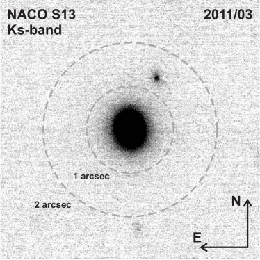
Figure 18: Fully reduced NACO image of POTS-1. The closest source found next to POTS-1 located about 1.3 arcsec north-west.

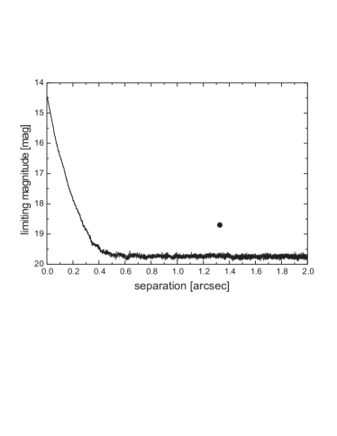
Figure 19: The achieved detection limit of our NACO observation is about 20 mag at an angular separation of 0.5 arcsec from POTS-1. Within 1 arcsec around the star, there is no object detected. The filled circle indicates the position and brightness of the closest source found next to POTS-1 (compare with Fig. 18).

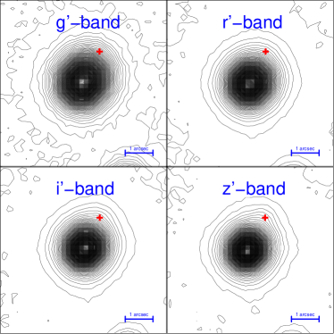
Figure 20: Isophotal contours for a stack of the 20 best seeing images in each of the four optical GROND bands. The 150 contours are equally spaced between 0 and the peak values of POTS-1. The object that is located 1.3 arcsec north-west (indicated by the red cross) is slightly distorting the contours of the redder bands $i^{\prime}$ and $z^{\prime}$ but not visible in the $g^{\prime}$ and $r^{\prime}$ bands.

3.4 Rejection of blend scenarios

Although the small amplitude of the RV variation, the bisector analysis presented in Section 3.1 and the high-resolution imaging presented in Section 3.3 confirm the planetary nature of POTS-1b, we perform an additional test to strengthen our result. Based on the light curves we rule out a scenario in which the POTS-1 system consists of an eclipsing binary system which is blended by a third object that is coincidentally in the line of sight or physically bound to the binary. In such a blend system, the transit depth would vary across the different bands if the spectral type of the blending star differs from the spectral type of the binary, since in each band the blending fraction will be different. If, on the other hand, the blending star is of a very similar spectral type, the shape of the transit would become inconsistent with the observations.
In a quantitative analysis similar to Torres et al. (2011), we simulated light curves of a large range of possible blend scenarios, i.e. foreground/background eclipsing binary and physical triplet systems with different amount of blending – quantified as the average fraction of third light in the observed bands – and different spectral types of the blending sources. To each of the blended light curves, we fitted an analytic eclipse model according to the equations of Mandel & Agol (2002) with quadratic limb-darkening coefficients taken as linear interpolations of the grid published by Claret & Bloemen (2011) and compared the $\chi^{2}$ of the blended to the unblended case. Fig. 21 shows the 1$\sigma$, 2$\sigma$ and 3$\sigma$ contours for all possible scenarios. For a small difference in $T_{eff}$ between POTS-1 and the blending source, an average third light fraction of up to $\sim$50 per cent is consistent with the observed light curves. Note however that in this case the radius of POTS-1b would be $\sim$1.33 R_Jup which is still well comparable to the radii of other extra-solar planets found in the past. In this sense, we can rule out all eclipsing binary scenarios with a fore- or background star that is contributing more than 50 per cent of the total light, which underlines the confirmation of the planetary nature of POTS-1b. Note that although this analysis shows that a blending light of up to 50 per cent is consistent with the light curves, there is no indication at all for a blend. We are therefore confident that all parameters derived in the previous sections are correct.
We investigated the possibility to apply the centroid-shift method (see e.g. Jenkins et al., 2010) to the GROND data as an additional test for a blend scenario; however, the faintness of POTS-1 and the low number of available out-of-transit points did not allow us to get any useful measurement.

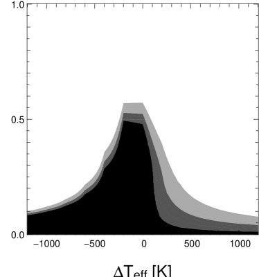
Figure 21: 1$\sigma$, 2$\sigma$ and 3$\sigma$ contours for all possible blend scenarios with a light contribution coming from the contaminating object quantified as the average third light fraction in all five available bands. Values of f${}_{3rd}>$ 50 per cent correspond to scenarios where the blending object is brighter than the eclipsing system, and values of f${}_{3rd}<$ 50 per cent correspond to scenarios where the eclipsing system is dominant. For effective temperature differences between POTS-1 and the blending star that are larger than a few hundred K, we can rule out a significant contamination. For very similar spectral types, up to $\sim$50 per cent contamination is still consistent with the light curves.

4 POTS-C2

In this section, we present our second best candidate POTS-C2. We list all $UBVRI$ magnitudes from the photometric calibration (see Section 2.1) and the 2MASS $JHK$ magnitude (Skrutskie et al., 2006) in Table 8. Since no H- and K-band error estimates were available in the 2MASS PSC, we list the typical 2MASS uncertainty for the given apparent brightness.
Using the broad-band photometry, we derived the stellar surface temperature $T_{\mathrm{eff}}$ making use of the synthetic fluxes calculated with marcs models (Gustafsson et al., 2008). We were able to derive an effective temperature of $T_{\mathrm{eff}}$ = 4900$\pm$400 K, a reddening of $E(B-V)$ = 0.43$\pm$0.08 mag and a distance of 2.3$\pm$1.0 kpc (see Fig. 22).
To determine the orbital and planetary parameters, we fitted analytical transit light-curve models according to the equations of Mandel & Agol (2002) with quadratic limb-darkening coefficients taken as linear interpolations of the grid published by Claret & Bloemen (2011). We make use of the spectral type estimate from SED fitting. The free parameters of the fits were period $P$, epoch $t_{0}$, inclination $i$ and planetary radius $R_{p}$. We also fitted a scale in order to renormalize the out-of-transit part of the light curve to 1.
In order to derive uncertainties of the system parameters, we minimized the $\chi^{2}$ on a grid centred on the previously found best-fitting parameters and searched for extreme grid points with $\Delta\chi^{2}$ = 1 when varying one parameter and simultaneously minimizing over the others. The best-fitting parameters and their error estimates are listed in Table 8. We show the folded light curves of POTS-C2 in Fig. 23 together with the best analytical model fit. Note that there are signs of a shallow secondary eclipse at phase value 0.5 which could indicate a significant brightness of POTS-C2b. However, the available data are not precise enough to make any claim in this direction.

POTS-C2 (2MASS 13373207–6650403)
Stellar parameters:
RA (J2000.0)	13h37m32$\aas@@fstack{s}$1
Dec. (J2000.0)	–66∘50′41′′
$U$	20.90$\pm$0.12 mag
$B$	19.90$\pm$0.04 mag
$V$	18.50$\pm$0.03 mag
$R$	17.70$\pm$0.06 mag
$I$	16.91$\pm$0.07 mag
$J$	15.93$\pm$0.12 mag
$H$	15.16$\pm$0.10 mag
$K$	15.09$\pm$0.14 maga
$d$	2.3$\pm$1.0 kpc
$E(B-V)$	0.43$\pm$0.08 mag
$T_{\mathrm{eff}}$	4900$\pm$400 K
Spectral type	K2V
Planetary and orbital parameters:
$P$	2.76303$\pm$2.0$\cdot 10^{-4}$ d
$t_{0}$	2454241.3652$\pm$0.0025 BJD
$R_{p}$	1.30$\pm$0.21 RJup
$i$	87$\aas@@fstack{\circ}$3$\pm$2$\aas@@fstack{\circ}$0
$a_{p}$	0.0349 AU
Light-curve and detection parameters:
S/N	38.0
$q$	0.031
$\Delta F$/$F$	0.024
No. of transits	3
No. of transit points	128
Baseline rms	0.0129

Table 8: Planetary, orbital and stellar parameters of the POTS-C2 system. Note that zero eccentricity has been assumed.

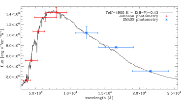
Figure 22: SED fitting for POTS-C2. The plot shows the comparison between marcs model theoretical fluxes calculated with $T_{\mathrm{eff}}$ = 4900 K and $\log g$ = 4.5 (our final set of fundamental parameters), taking into account a reddening of E($B$-$V$) = 0.43 mag, with the Johnson–Cousins $UBVRI$ photometry (red crosses) and 2MASS photometry (blue asterisks).

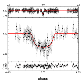
Figure 23: Folded R-band light curve of POTS-C2. The red line shows the best-fitting model with the parameters listed in Table 8.

5 Conclusions

We have presented the results of the POTS, a pilot project aiming at the detection of transiting planets in the Galactic disc. Using the difference imaging approach, we produced high-precision light curves of 16000 sources with several thousands of data points and a high cadence of $\sim$2 min. All light curves are publicly available.
A detailed analysis of the POTS light curves revealed two very interesting planet candidates. With extensive spectroscopic and photometric follow-up observations, we were able to derive the parameters of the POTS-1 system and confirm its companion as a planet with a mass of 2.31$\pm$0.77 M_Jup and a radius of 0.94$\pm$0.04 R_Jup. This would lead to the conclusion that POTS-1b has a relatively high but not unusual density.
Due to the specific dates of the RV observations, there is a possibility that the RV variation is caused by a log-term linear trend due to an undetected stellar companion of POTS-1 in which case the true RV amplitude and the true mass of POTS-1b would be lower. Also there could be a systematic offset between the observations taken in the two different instrument configurations. As a consequence, the true RV variation could be actually smaller or larger than that estimated in our analysis and the true mass and density of POTS-1b could be lower or higher. We therefore analysed the RV data of the two instrumental configurations independently (see Section 3.1.4) and found best planetary masses of M_p = 1.91${}^{+1.30}_{-1.19}$ and 0.38${}^{+0.86}_{-0.38}$ M_Jup, respectively, which are both in the planetary regime.
In order to rule out a blend scenario, we analysed the bisector span as a function of orbital phase which showed no significant variations although the errors on the measurements are rather large. In addition, we investigate the possibility to rule out a blend scenario based on the light curves alone. We were able to set an upper limit of $\sim$50 per cent on the light coming from a blending source.
Using high-resolution imaging we identified a contaminating source $\sim$1.3 arcsec north-west of POTS-1; however, the contamination in the $K_{s}$ band is as low as $\sim$2 per cent. There is no indication for any additional bright blending source.
Despite its faintness, the parameters of the POTS-1 system, i.e. planetary radius and stellar density, inclination, orbital period and epoch, are very well constraint thanks to the high-precision observations with GROND and the long baseline between the WFI and GROND data sets.
Among all transiting planets discovered so far, POTS-1b is orbiting one of the coolest stars and the period of 3.16 d is one of the longest periods of all transiting planets detected around mid/end-K dwarfs and M dwarfs.
In Section 4, we presented an unconfirmed candidate found in the POTS, i.e. POTS-C2b, which has a period of 2.76303$\pm$2.0 $\times$ 10^-4 d. The host star has an effective temperature of 4900$\pm$400 K as derived from SED fitting, and the best-fitting radius of the planet candidate is 1.30$\pm$0.21 R_Jup. Our follow-up observations of POTS-1 have shown that the confirmation of a planet orbiting a faint star can be difficult and costly with currently available instrumentation. In the optical wavelength regime, POTS-C2 is $\sim$0.6 mag fainter than POTS-1. Nevertheless, POTS-C2b may be an interesting target for follow-up studies in the future.
As a final remark, we want to point out that the main reason for not finding any candidates around brighter stars is the limited survey area of this pilot project.

References

- Adelman-McCarthy et al. (2007) Adelman-McCarthy J. K. et al., 2007, ApJS, 172, 634
- Alard & Lupton (1998) Alard C., Lupton R. H., 1998, ApJ, 503, 325
- Amôres & Lépine (2005) Amôres E. B., Lépine J. R. D., 2005, AJ, 130, 659
- Asplund et al. (2009) Asplund M., Grevesse N., Sauval A. J., Scott P., 2009, ARA&A, 47, 481
- Auvergne et al. (2009) Auvergne M. et al., 2009, A&A, 506, 411
- Baade et al. (1999) Baade D. et al., 1999, The Messenger, 95, 15
- Bakos et al. (2004) Bakos G., Noyes R. W., Kovács G., Stanek K. Z., Sasselov D. D., Domsa I., 2004, PASP, 116, 266
- Bakos et al. (2006) Bakos, G. Á., Pál, A., Latham, D. W., Noyes, R. W., Stefanik, R. P., 2006, ApJ, 641, L57
- Baraffe et al. (1998) Baraffe I., Chabrier G., Allard F., Hauschildt P. H., 1998, A&A, 337, 403
- Barbieri (2007) Barbieri M., 2007, in Afonso C., Weldrake D., Henning T., eds, ASP Conf. Ser., Vol. 366, Transiting Extrapolar Planets Workshop. Astron. Soc. Pac., San Francisco, p. 78
- Batalha et al. (2012) Batalha N. M. et al., 2013, ApJS, 204, 24
- Beatty & Gaudi (2008) Beatty T. G., Gaudi B. S., 2008, ApJ, 686, 1302
- Berta et al. (2012) Berta Z. K. et al., 2012, ApJ, 747, 35
- Bertin & Arnouts (1996) Bertin E., Arnouts S., 1996, A&AS, 117, 393
- Binney & Merrifield (1998) Binney J., Merrifield M., 1998, Galactic Astronomy. Princeton Univ. Press, Princeton, NJ
- Borucki et al. (2010) Borucki W. J. et al., 2010, Science, 327, 977
- Capaccioli, Mancini & Sedmak (2002) Capaccioli M., Mancini D., Sedmak G., 2002, in Tyson J. A., Wolff S., eds, Proc. SPIE Conf. Ser. Vol. 4836, Survey and Other Telescope Technologies and Discoveries. SPIE, Bellingham, p. 43
- Charbonneau et al. (2000) Charbonneau D., Brown T. M., Latham D. W., Mayor M., 2000, ApJ, 529, L45
- Charbonneau et al. (2005) Charbonneau D. et al., 2005, ApJ, 626, 523
- Claret & Bloemen (2011) Claret A., Bloemen S., 2011, A&A, 529, A75
- Colón, Ford & Morehead (2012) Colón K. D., Ford E. B., Morehead R. C., 2012, MNRAS, 426, 342
- de Mooij et al. (2012) de Mooij E. J. W. et al., 2012, A&A, 538, A46
- Dekker et al. (2000) Dekker H., D’Odorico S., Kaufer A., Delabre B., Kotzlowski H., 2000, in Iye M., Moorwood A. F., eds, Proc. SPIE Conf. Ser. Vol. 4008, Optical and IR Telescope Instrumentation and Detectors. SPIE, Bellingham, p. 534
- Devillard (2001) Devillard N., 2001, in Harnden Jr. F. R., Primini F. A., Payne H. E., eds, ASP Conf. Ser. Vol. 238, Astronomical Data Analysis Software and Systems X. Astron. Soc. Pac., San Francisco, p. 525
- Dotter et al. (2008) Dotter A., Chaboyer B., Jevremović D., Kostov V., Baron E., Ferguson J. W., 2008, ApJS, 178, 89
- Fossati et al. (2009) Fossati L., Ryabchikova T., Bagnulo S., Alecian E., Grunhut J., Kochukhov O., Wade G., 2009, A&A, 503, 945
- Fressin et al. (2007) Fressin F., Guillot T., Morello V., Pont F., 2007, A&A, 475, 729
- Fukui et al. (2011) Fukui A. et al., 2011, PASJ, 63, 287
- Gössl & Riffeser (2002) Gössl C. A., Riffeser A., 2002, A&A, 381, 1095
- Greiner et al. (2008) Greiner J. et al., 2008, PASP, 120, 405
- Gustafsson et al. (2008) Gustafsson B., Edvardsson B., Eriksson K., Jørgensen U. G., Nordlund Å., Plez B., 2008, A&A, 486, 951
- Irwin et al. (2009) Irwin J., Charbonneau D., Nutzman P., Falco E., 2009, in Pont F., Sasselov D., Holman M., eds, Proc. IAU Symp. Vol. 253, Transiting Planets. Cambridge Univ. Press, Cambridge, p. 37
- Jenkins et al. (2010) Jenkins J. M. et al., 2010, ApJ, 724, 1108-1119
- Jester et al. (2005) Jester S. et al., 2005, AJ, 130, 873
- Koppenhoefer (2009) Koppenhoefer, J., 2009, PhD thesis, Ludwig Maximilians University Munich
- Koppenhoefer et al. (2009) Koppenhoefer J., Afonso C., Saglia R. P., Henning T., 2009, A&A, 494, 707
- Koppenhoefer, Saglia & Riffeser (2013) Koppenhoefer J., Saglia R. P., Riffeser A., 2013, Exp. Astron., 35, 329
- Kovács, Zucker & Mazeh (2002) Kovács G., Zucker S., Mazeh T., 2002, A&A, 391, 369
- Kovács et al. (2013) Kovács G. et al., 2013, MNRAS, 433, 889
- Kuijken et al. (2002) Kuijken K. et al., 2002, The Messenger, 110, 15
- Kupka et al. (1999) Kupka F., Piskunov N., Ryabchikova T. A., Stempels H. C., Weiss W. W., 1999, A&AS, 138, 119
- Kurucz (1993) Kurucz R., 1993, ATLAS9 Stellar Atmosphere Programs and 2 km/s grid. Kurucz CD-ROM No. 13. Smithsonian Astrophysical Observatory, Cambridge, p. 13
- Landolt (1992) Landolt A. U., 1992, AJ, 104, 340
- Law et al. (2011) Law N. M., Kraus A. L., Street R. R., Lister T., Shporer A., Hillenbrand L. A., Palomar Transient Factory Collaboration, 2011, in Johns-Krull C., Browning M. K., West A. A., eds, ASP Conf. Ser. Vol. 448, 16th Cambridge Workshop on Cool Stars, Stellar Systems, and the Sun. Astron. Soc. Pac., San Francisco, p. 1367
- Lendl et al. (2010) Lendl M., Afonso C., Koppenhoefer J., Nikolov N., Henning T., Swain M., Greiner J., 2010, A&A, 522, A29
- Lenzen et al. (2003) Lenzen R. et al., 2003, in Iye M., Moorwood A. F. M., eds, Proc. SPIE Conf. Ser. Vol. 4841, Instrument Design and Performance for Optical/Infrared Ground-based Telescopes. SPIE, Bellingham, p. 944
- Maciejewski et al. (2010) Maciejewski G. et al., 2010, MNRAS, 407, 2625
- Mandel & Agol (2002) Mandel K., Agol E., 2002, ApJ, 580, L171
- McCullough et al. (2005) McCullough P. R., Stys J. E., Valenti J. A., Fleming S. W., Janes K. A., Heasley J. N., 2005, PASP, 117, 783
- Meeus (1982) Meeus J., 1982, Astronomical Formulae for Calculators. Willmann-Bell, Richmond, VA, p. 43
- Morel, & Miglio (2012) Morel, T. and Miglio, A., 2012, MNRAS, 419, 34
- Morton & Johnson (2011) Morton T. D., Johnson J. A., 2011, ApJ, 738, 170
- Nikolov et al. (2012) Nikolov N., Henning T., Koppenhoefer J., Lendl M., Maciejewski G., Greiner J., 2012, A&A, 539, A159
- O’Donovan et al. (2007) O’Donovan F. T. et al., 2007, ApJ, 663, L37
- Pasquini et al. (2002) Pasquini L. et al., 2002, The Messenger, 110, 1
- Pasquini et al. (2012) Pasquini L. et al., 2012, A&A, 545, A139
- Pavlenko (1997) Pavlenko Y. V., 1997, Ap&SS, 253, 43
- Pavlenko (2003) Pavlenko Y. V., 2003, Astron. Rep., 47, 59
- Pavlenko et al. (2012) Pavlenko Y. V., Jenkins J. S., Jones H. R. A., Ivanyuk O., Pinfield D. J., 2012, MNRAS, 422, 542
- Piskunov et al. (1995) Piskunov N. E., Kupka F., Ryabchikova T. A., Weiss W. W., Jeffery C. S., 1995, A&AS, 112, 525
- Pollacco et al. (2006) Pollacco D. L. et al., 2006, PASP, 118, 1407
- Pont, Zucker & Queloz (2006) Pont F., Zucker S., Queloz D., 2006, MNRAS, 373, 231
- Queloz et al. (2001) Queloz D. et al., 2001, A&A, 379, 279
- Riffeser, Seitz & Bender (2008) Riffeser A., Seitz S., Bender R., 2008, ApJ, 684, 1093
- Robin et al. (2003) Robin, A. C., Reylé, C., Derrière, S. and Picaud, S., 2003, A&A, 409, 523
- Rousset et al. (2003) Rousset G. et al., 2003, in Wizinowich P. L., Bonaccini D., eds, Proc. SPIE Conf. Ser. Vol. 4839, Adaptive Optical System Technologies II. SPIE, Bellingham, p. 140
- Ryabchikova et al. (1999) Ryabchikova T. A., Piskunov N. E., Stempels H. C., Kupka F., Weiss W. W., 1999, Phys. Scr. T, 83, 162
- Sahu et al. (2006) Sahu K. C. et al., 2006, Nature, 443, 534-540
- Schlegel, Finkbeiner & Davis (1998) Schlegel D. J., Finkbeiner D. P., Davis M., 1998, ApJ, 500, 525
- Skrutskie et al. (2006) Skrutskie M. F. et al., 2006, AJ, 131, 1163
- Snellen et al. (2009) Snellen I. A. G. et al., 2009, A&A, 497, 545
- Snellen et al. (2007) Snellen I. A. G., van der Burg R. F. J., de Hoon M. D. J., Vuijsje F. N., 2007, A&A, 476, 1357
- Stetson (1987) Stetson P. B., 1987, PASP, 99, 191
- Stetson (2000) Stetson P. B., 2000, PASP, 112, 925
- Tamuz, Mazeh & Zucker (2005) Tamuz O., Mazeh T., Zucker S., 2005, MNRAS, 356, 1466
- Tomaney & Crotts (1996) Tomaney A. B., Crotts A. P. S., 1996, AJ, 112, 2872
- Torres et al. (2011) Torres G. et al., 2011, ApJ, 727, 24
- Tsymbal (1996) Tsymbal V., 1996, in Adelman S. J., Kupka F., Weiss W. W., eds, ASP Conf. Ser. Vol. 108, M.A.S.S.: Model Atmospheres and Spectrum Synthesis. Atron. Soc. Pac., San Francisco, p. 198
- Udalski et al. (2004) Udalski A., Szymanski M. K., Kubiak M., Pietrzynski G., Soszynski I., Zebrun K., Szewczyk O., Wyrzykowski L., 2004, Acta Astron., 54, 313
- Udalski et al. (2008) Udalski A., Szymanski M. K., Soszynski I., Poleski R., 2008, Acta Astron., 58, 69
- Valenti & Fischer (2005) Valenti J. A., Fischer D. A., 2005, ApJS, 159, 141
- Valentijn et al. (2007) Valentijn E. A. et al., 2007, in Shaw R. A., Hill F., Bell D. J., eds, ASP Conf. Ser. Vol. 376, Astronomical Data Analysis Software and Systems XVI. Astron. Soc. Pac., San Francisco, p. 491
- Winn et al. (2009) Winn J. N., Johnson J. A., Albrecht S., Howard A. W., Marcy G. W., Crossfield I. J., Holman M. J., 2009, ApJ, 703, L99
- Young (1967) Young, A. T., 1967, AJ, 72, 747