Localizability of Wireless Sensor Networks:
Beyond Wheel Extension

Abstract

A network is called localizable if the positions of all the nodes of the network can be computed uniquely. If a network is localizable and embedded in plane with generic configuration, the positions of the nodes may be computed uniquely in finite time. Therefore, identifying localizable networks is an important function. If the complete information about the network is available at a single place, localizability can be tested in polynomial time. In a distributed environment, networks with trilateration orderings (popular in real applications) and wheel extensions (a specific class of localizable networks) embedded in plane can be identified by existing techniques. We propose a distributed technique which efficiently identifies a larger class of localizable networks. This class covers both trilateration and wheel extensions. In reality, exact distance is almost impossible or costly. The proposed algorithm based only on connectivity information. It requires no distance information.

Key words:  Wireless sensor networks, graph rigidity, localization, localizable networks, distributed localizability testing.

1 Introduction

A sensor is a small sized and low powered electronic device with limited computational and communicating capability. A sensor network is a network containing some ten to millions of sensors. Wireless sensor networks (WSNs) have wide-ranging applications in problems such as traffic control, habitat monitoring, battlefield surveillance (e.g., intruder detection or giving assistance to mobile soldiers etc.), fire detection for monitoring forest-fires, disaster management, to alert the appearance of phytoplankton under the sea, etc. WSNs can help in gathering information from regions, where human access is difficult. To react to an event detected by a sensor, the knowledge about the position of the sensor is necessary. Sensor deployment may be random. For example, they may be dropped from an air vehicle with no pre-defined infra-structure. In such cases, the positions of the sensors are completely unknown to start with. The problem of finding the positions of nodes in a network is known as network localization.

A wireless ad-hoc network embedded in $\mathbb{R}^{m}$ ($m$-dimensional Euclidean space) may be represented by a distance graph $G=(V,E,d)$ whose vertices represent computing devices. A pair of nodes, $\{u,v\}\in E$ if and only if the Euclidean distance between $u$ and $v$ ($d(u,v)=|u-v|$) is known. Determining the coordinates of vertices in an embedding of $G$ in $\mathbb{R}^{m}$ may be considered as graph realization problem [1, 2, 3, 4]. A realization of a distance graph $G=(V,E,d)$ in $\mathbb{R}^{m}$ is an injective mapping $p:V\rightarrow\mathbb{R}^{m}$ such that $|p(u)-p(v)|=d(u,v)$, $\forall\{u,v\}\in E$ (i.e., one-to-one assignment of coordinates $(x_{1},\ldots,x_{m})\in\mathbb{R}^{m}$ to every vertex in $V$ so that the $d(u,v)$ represents the distance between $u$ and $v$. The pair $(G,p)$ is called a framework of $G$ in $\mathbb{R}^{m}$. Two frameworks $(G,p)$ and $(G,q)$ are congruent if $|p(u)-p(v)|=|q(u)-q(v)|$, $\forall u,v\in V$ (i.e., preserving the distances between all pairs of vertices). A framework $(G,p)$ is rigid, if it has no smooth deformation [5] preserving the edge lengths. The distance graph $G$ is generically globally rigid [5], if all realizations with generic configurations (set of points with coordinates not being algebraically dependent) are congruent. A set $A=\{\alpha_{1},\ldots,\alpha_{m}\}$ of real numbers is algebraically dependent if there is a non-zero polynomial $h$ with integer coefficients such that $h(\alpha_{1},\ldots,\alpha_{m})=0$. The graph $G$ is termed as globally rigid, if all realizations of $G$ are congruent. In this work, we consider realizations of a distance graph only in plane with generic configurations. Here onwards, all the discussions and results are concerned only in $\mathbb{R}^{2}$.

In real applications, positions of the nodes of a network may either be 1) estimated [6, 7, 8, 9, 10] within some tolerable error level or 2) uniquely realized. If all realizations of a network are congruent, the network is called localizable. A distance graph is localizable if and only if it is globally rigid. Starting from three anchors (nodes with known unique position), all the nodes in a globally rigid graph can be uniquely realized. If the nodes cannot be localized using the given information, in several applications location estimation may serve well. Localization of a network is $NP$-hard [11] even when it is localizable [12]. Jackson and Jordán [12] proved that a graph is globally rigid, if and only if it is $3$-connected and redundantly rigid. A graph is $3$-connected, if at least three vertices must be removed to make the graph disconnected. A graph is redundantly rigid, if it remains rigid after removing any edge. Localizability of a graph can be answered in polynomial time [12] by testing the 3-connectivity and redundant rigidity when complete network wide information is available in a single machine. To gather complete network information in a single machine is infeasible or very costly. On the contrary, finding methods to recognize globally rigid graphs in distributed environments based on local information is still a challenging problem [13].

The rest of the paper is organized as follows. Section 2 describes motivation and contribution of this work. Section 3 introduces some classes of localizable graphs which include trilateration graph and wheel extension as their special cases. Section 4 defines the problem. It also describes a mapping of the problem into triangle bar recognition. Section 5 describes the proposed distributed algorithm of localizability testing. Section 6 proves correctness and performance analysis of the algorithm. Finally, we conclude in Section 7.

2 Background and our contribution

The most commonly used technique for localization is trilateration [14, 15]. It efficiently localizes a trilateration graph starting from three anchors. A trilateration graph is a graph with a trilateration ordering, $\pi=(u_{1},u_{2},\ldots,u_{n})$ where $u_{1}$, $u_{2}$, $u_{3}$ form a $K_{3}$ and every $u_{i}$ ($i>3$) is adjacent to at least three nodes before $u_{i}$ in $\pi$. However, not all localizable networks admit trilateration ordering.

(a) Wheel graph

(b) Wheel

extension

(c) Triangle cycle

(d) Triangle

circuit

(e) Triangle bridge

(f) Triangle net

Figure 1: Examples of some localizable graphs having different properties

Fig. 1 (a) and 1 (b) respectively show a wheel graph and a wheel extension graph which have no trilateration ordering. A wheel $W_{n}$ with $n$ vertices is a graph consisting of a cycle with $n-1$ nodes and a vertex which is adjacent to all vertices on the cycle. A wheel extension is a graph having an ordering $\pi=(u_{1},u_{2},\ldots,u_{n})$ of nodes where $u_{1}$, $u_{2}$, $u_{3}$ form a $K_{3}$ and each $u_{i}$, $i>3$, lies in a wheel subgraph containing at least three nodes before $u_{i}$ in $\pi$. A wheel extension is generically globally rigid and its localizability can be identified efficiently and distributedly [13]. However, there are many more localizable graphs which do not have wheel extensions. For example, Fig. 1 (c), 1 (d), 1 (e) and 1 (f) are examples of graphs which are generically globally rigid, but do not have wheel extensions.

The main contributions of this paper are as follows. It introduces some elementary class of localizable graphs triangle cycle, triangle circuit, triangle bridge, triangle notch and triangle net. Using these elementary classes of graphs, we build up a new family of generically globally rigid graphs called triangle bar. Trilateration graphs and wheel extensions are special cases of triangle bars. We propose an efficient distributed algorithm that recognizes triangle bars starting from a $K_{3}$ based only on connectivity information. It requires no distance information. In real applications, exact node distance is impossible or costly. However, several localizable graphs still fall outside the class triangle bar. To the best of our knowledge, distributedly recognizing an arbitrary localizable network still is an open problem.

3 Rigidity and localizability of triangle bar

Unique realizability is closely related to graph rigidity [1, 2]. The realizability testing of a distance graph $G=(V,E,d)$ is $NP$-hard [11]. We expect data are consistent to have a realization, if the distance information is collected from an actual deployment of devices. A realization of $G$ may be visualized as a frame constructed by a finite set of hinged rods. The junctions and free ends are considered as vertices of the realization and rods as the edges. With perturbation on the frame, we may have a different realization preserving the edge distances. The realizations obtained by flipping, rotating or shifting the whole structure are congruent. By flip, rotation or shift on a realization, we mean a part of the realization is flipped, rotated or shifted. If two globally rigid graphs in $\mathbb{R}^{2}$ share exactly one vertex in common, one of them may be rotated around the common vertex keeping the other fixed. Such a vertex is called a joint. If two globally rigid graphs in $\mathbb{R}^{2}$ share exactly two vertices, rotation about these vertices is no longer possible, but one of the graphs may be flipped, about the line joining the two common vertices, keeping the other fixed. This pair of vertices is called a flip.

Lemma 1 ([16])

If two globally rigid subgraphs, $B_{1}$ and $B_{2}$, of a graph embedded in plane share at least three non-collinear vertices, then $B_{1}\cup B_{2}$ is globally rigid.

In this section, we formally introduce some elementary classes of localizable graphs: triangle cycle, triangle circuit, triangle bridge, triangle notch, triangle net. Using these elementary classes, a larger class of localizable graphs triangle bar is formally defined.

3.1 Triangle cycle, triangle circuit and triangle bridge

Let ${\cal T}=(T_{1},T_{2},\ldots,T_{m})$ be a sequence of distinct triangles such that for every $i$, $2\leq i\leq m-1$, $T_{i}$ shares two distinct edges with $T_{i-1}$ and $T_{i+1}$. Such a sequence ${\cal T}$ of triangles is called a triangle stream (Fig. 2 (a)).

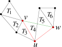
(a) Triangle chain

(b) triangle cycle

(c) triangle circuit

(d) triangle bridge

Figure 2: Examples of triangle chain, triangle cycle, triangle circuit and triangle bridge

$G({\cal T})$ is the graph constructed by taking the union of the $T_{i}$s in ${\cal T}$. A node $u$ of a triangle $T_{i}$ is termed a pendant of $T_{i}$, if the edge opposite to $u$ in $T_{i}$ is shared by another triangle in ${\cal T}$. This shared edge is called an inner side of $T_{i}$. Each triangle $T_{i}$ has at least one edge which is not shared by another triangle in ${\cal T}$. Such a non-shared edge is called an outer side of $T_{i}$. In Fig. 2 (a), $T_{4}=\{u,v,w\}$ has two pendants $v$ and $w$. It has two inner sides $uw$ and $uv$ and one outer side $vw$. If each of $T_{1}$ and $T_{m}$ has unique and distinct pendants, then $G({\cal T})$ is termed a triangle chain. Fig. 2 (a) shows an example of triangle chain. By construction, a triangle chain involves only flips; hence rigid. If $T_{1}$ and $T_{m}$ share a common edge other than those shared with $T_{2}$ and $T_{m-1}$, then the union $G({\cal T})$ is called a triangle cycle. In a triangle cycle, each triangle has exactly two inner and one outer sides. Fig. 2 (b) shows an example of a triangle cycle. Every wheel graph is a triangle cycle.

If $G({\cal T})$ is not a triangle cycle and $T_{1}$ and $T_{m}$ have a unique pendant in common, then $G({\cal T})$ is called a triangle circuit (Fig. 2 (c)). The common pendant is called a circuit knot. $x$ is the circuit knot of the triangle circuit. Let ${\cal T}=(T_{1},T_{2},\ldots,T_{m})$ be a triangle stream corresponding to a triangle chain. $T_{1}$ and $T_{m}$ have unique and distinct pendants. We connect these pendants by an edge $e$. $G({\cal T})\cup\{e\}$ is called a triangle bridge (Fig. 2 (d)). The edge $e$ is called the bridging edge. The length of a triangle stream ${\cal T}$ is the number of triangles in it and is denoted by $l({\cal T})$.

Lemma 2

1) Every triangle cycle has a spanning wheel or triangle circuit (a wheel or triangle circuit which is a spanning subgraph of the triangle cycle). 2) Every triangle circuit has a spanning triangle bridge (a triangle bridge which is a spanning subgraph of the triangle circuit).

Proof

See Appendix 0.A.1 for the first part. For the second part, see Appendix 0.A.2. ∎

We have seen that a rigid realization in $\mathbb{R}^{2}$ may have flip ambiguity, i.e., it may yield another configuration by applying flip operation only. In $\mathbb{R}^{2}$, if a rigid realization admits no flip ambiguity, then it is globally rigid. Using this, we shall prove the generically global rigidity as follows.

Lemma 3

Triangle cycle, circuit and bridge are generically globally rigid.

Proof

A triangle cycle has a spanning wheel or triangle circuit (Lemma 2). A wheel graph is generically globally rigid. A triangle circuit always has a spanning triangle bridge (Lemma 2). If we can prove that a triangle bridge is generically globally rigid, the result will follow.

Let $G({\cal T})$ be a triangle bridge with the triangle stream ${\cal T}=(T_{1},T_{2},\ldots,T_{n})$ and the bridging edge $e$. Consider a generic configuration of $G({\cal T})$ (Fig. 3). Note that $G({\cal T})$ contains $n+2$ nodes.

Figure 3: A generic configuration of a triangle bridge $G({\cal T})$

$G({\cal T})-e$ is a spanning triangle chain (a triangle chain which is a spanning subgraph of the triangle bridge) of $G({\cal T})$. Since $G({\cal T})-e$ can only have flips, i.e., no smooth deformation. Therefore, $G({\cal T})$ also admits no smooth deformation.

Consider a different realization of $G({\cal T})$ obtained from the current realization through a sequence of flip operations. Without loss of generality, we assume that $T_{1}$ remains fixed with positions $(x_{0},y_{0})$, $(x_{1},y_{1})$ and $(x_{2},y_{2})$ for $w$ and two other nodes in $T_{1}$ respectively. If $T_{2}$ is involved in a flip, then the only possibility is the flip that is taken with respect to the inner edge with $T_{1}$. Only one point of $T_{2}$ changes its position. Let $(x_{3},y_{3})$ and $(x_{3}^{\prime},y_{3}^{\prime})$ be the positions of this point in the original and the modified configuration respectively. From elementary coordinate geometry, $x_{3}^{\prime}$ and $y_{3}^{\prime}$ can be expressed in the form of $\frac{\phi_{3}}{\psi_{3}}$ and $\frac{\xi_{3}}{\eta_{3}}$ where $\phi_{3}$, $\psi_{3}$, $\xi_{3}$ and $\eta_{3}$ are non-zero polynomials of $x_{1}$, $y_{1}$, $x_{2}$, $y_{2}$, $x_{3}$ and $y_{3}$ with integer coefficients such that $\psi_{3}\neq 0$ and $\eta_{3}\neq 0$. Once, the positions of $T_{1}$ and $T_{2}$ in the second configuration are computed (fixed) then only one point of $T_{3}$ may need to be computed. This node again may be involved in a flip with respect to the inner edge of $T_{2}$. If $(x_{4},y_{4})$ and $(x_{4}^{\prime},y_{4}^{\prime})$ are the positions of this point in the original and modified configurations respectively, $x_{4}^{\prime}$ and $y_{4}^{\prime}$ can be expressed in the form of $\frac{\phi_{4}^{\prime}}{\psi_{4}^{\prime}}$ and $\frac{\xi_{4}^{\prime}}{\eta_{4}^{\prime}}$ where $\phi_{4}^{\prime}$, $\psi_{4}^{\prime}$, $\xi_{4}^{\prime}$ and $\eta_{4}^{\prime}$ are non-zero polynomials of $x_{2}$, $y_{2}$, $x_{3}^{\prime}$, $y_{3}^{\prime}$, $x_{4}$ and $y_{4}$ with integer coefficients such that $\psi_{4}^{\prime}\neq 0$ and $\eta_{4}^{\prime}\neq 0$. In this expression, if we substitute $x_{3}^{\prime}$ and $y_{3}^{\prime}$ by expressions involving $x_{1}$, $y_{1}$, $x_{2}$, $y_{2}$, $x_{3}$ and $y_{3}$ (obtained from the previous equations), $x_{4}^{\prime}$ and $y_{4}^{\prime}$ can be expressed in the form of $\frac{\phi_{4}}{\psi_{4}}$ and $\frac{\xi_{4}}{\eta_{4}}$ where $\phi_{4}$, $\psi_{4}$, $\xi_{4}$ and $\eta_{4}$ are non-zero polynomials of $x_{1}$, $y_{1}$, $x_{2}$, $y_{2}$, $x_{3}$, $y_{3}$, $x_{4}$ and $y_{4}$ with integer coefficients such that $\psi_{4}\neq 0$ and $\eta_{4}\neq 0$. Proceeding in this way, finally $(x_{n+1}^{\prime},y_{n+1}^{\prime})$, the position of $v$, can be expressed in the form of $\frac{\phi}{\psi}$ and $\frac{\xi}{\eta}$ where $\phi$, $\psi$, $\xi$ and $\eta$ are non-zero polynomials of $x_{i}$s and $y_{i}$s, $1\leq i\leq n+1$, the coordinates of the nodes in the first configuration, with integer coefficients such that $\psi\neq 0$ and $\eta\neq 0$.

Since $v$ and $w$ are adjacent, $d(w,v)$ (the Euclidean distance between $w$ and $v$) remains preserved in both configurations. In terms of the coordinates,

$$(x_{n+1}^{\prime}-x_{0})^{2}+(y_{n+1}^{\prime}-y_{0})^{2} = (x_{n+1}-x_{0})^{2}+(y_{n+1}-y_{0})^{2},$$

$$\eta^{2}(\phi-x_{0}\psi)^{2}+\psi^{2}(\xi-y_{0}\eta)^{2} = \eta^{2}\psi^{2}(x_{n+1}-x_{0})^{2}+\eta^{2}\psi^{2}(y_{n+1}-y_{0})^{2}.$$

So the coordinates in the original configuration are algebraically dependent. It contradicts that the configuration is generic. Therefore, no flip is possible. ∎

3.2 Triangle notch and triangle net

Consider a sequence ${\cal T}=(T_{1},T_{2},\ldots,T_{m})$ of triangles. Suppose, for $i=2$, $3$, $\cdots$, $m$, each $T_{i}$ shares exactly one edge with exactly one $T_{j}$, $1\leq j<i$. The node opposite to this sharing edge is called a pendant of $T_{i}$ in ${\cal T}$. Fig. 5 shows an example of such a sequence and $x$ is a pendant of $T_{2}$. $T_{1}$ has no pendant.

Figure 4: Triangle tree

Figure 5: (a) Triangle tree (b) $u$ and $v$ are Extended nodes

For $2\leq i\leq m$, each $T_{i}$ has exactly one pendant in $\cal T$. The graph $G({\cal T})$ corresponding to such a sequence $\cal T$, is called a triangle tree. Fig. 5 is an example of a triangle tree with $11$ triangles. $G({\cal T})$ contains no triangle cycle. Otherwise, there always exists a $T_{j}$ which shares two edges with some triangles before $T_{j}$ in ${\cal T}$. If a triangle $T_{i}$ shares no edge with $T_{j}$, $j>i$, is called a leaf triangle. A leaf triangle shares exactly one edge with other triangles in ${\cal T}$. It has a unique pendant, called a leaf knot. $T_{5}$, $T_{7}$ and $T_{11}$ are leaf triangles and $u$, $v$ and $w$ are leaf knots. By construction, any realization of a triangle tree is rigid.

Definition 1

Let $G({\cal T})$ be a triangle tree. A node $v$, outside $G({\cal T})$, is called an extended node of $G({\cal T})$, if $v$ is adjacent to at least three nodes, each being $i)$ a pendant in $G({\cal T})$; or $ii)$ an extended node of $G({\cal T})$. Each of the edges which connect the extended node to a pendant or an extended knot of $G({\cal T})$ is called an extending edge.

Fig. 5 (a) is a triangle tree, say $G({\cal T})$. Fig. 5 (b) consists of a replica of the graph in Fig. 5 (a) and some more nodes and edges. Fig. 5 (a) does not contain $u$ of Fig. 5 (b). $u$ is adjacent to three pendants $w$, $x$ and $z$. So $u$ is an extended node of $G({\cal T})$. The edges $uw$, $ux$ and $uz$ are the extending edges of $u$. Similarly, $v$ is adjacent to an extended node $u$ and two pendants $s$ and $y$. So $v$ is also an extended node of $G({\cal T})$; where $vu$, $vs$ and $vy$ are the extending edges.

Definition 2

A graph $G$ is called a triangle notch, if it can be generated from a triangle tree $G^{\prime}({\cal T})$, where $G^{\prime}$ is proper subgraph of $G$, by adding only one extended node $v$ where all the leaf knots of $G^{\prime}({\cal T})$ are adjacent to $v$. The extended node $v$ is called the apex of $G$.

Fig. 6 (b) shows an example of a triangle notch with the apex $v$. The triangle tree from which it is generated is separately shown in Fig. 6 (a).

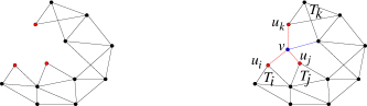
(a)                                 (b)

Figure 6: (a) Triangle tree $G({\cal T})$ (b) Triangle notch with apex $v$

Lemma 4

A triangle notch is generically globally rigid.

Proof

See Appendix 0.A.3. ∎

Lemma 5

Let $G$ be a graph obtained from a triangle tree $G^{\prime}({\cal T})$ by adding extended nodes, where $G^{\prime}$ is a proper subgraph of $G$. Any extended node along with all pendants and extended nodes adjacent to it lie in a generically globally rigid subgraph.

Proof

If the extended node $v$ is adjacent to only pendants of $G^{\prime}({\cal T})$, then these pendants are leaf knots of some triangle tree $G^{\prime\prime}({\cal T^{\prime}})$ where the triangles of ${\cal T^{\prime}}$ are all taken from ${\cal T}$. $G^{\prime\prime}({\cal T^{\prime}})\cup\{v\}$ forms a triangle notch. Fig. 7 (a) shows an example of such a case.

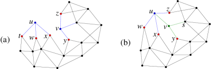
Figure 7: $u$ and $v$ are extended nodes where (a) $u$, $v$ are adjacent to pendants only, (b) $u$, $v$ are adjacent to both pendant and extended nodes

By Lemma 4, $G^{\prime\prime}({\cal T^{\prime}})\cup\{v\}$ is generically globally rigid. Now consider the case when $v$ is adjacent to at least one extended node. Let $u$ be an extended node which is adjacent to $v$ (Fig. 7 (b)). Since $u$ is also an extended node of $G^{\prime}({\cal T})$, we assume that $u$ lies in a generically globally rigid subgraph $G_{1}$ of $G$ and is generated from a triangle tree $G^{\prime\prime}({\cal T^{\prime}})$ by adding extended nodes (including $u$), where ${\cal T^{\prime}}$ contains triangle only from ${\cal T}$. Consider a generic configuration $\cal P$ of $G_{1}$. If $G_{1}$ admits any flip operation in $\cal P$ to yield a different configuration ${\cal P}^{\prime}$, then proceeding in a manner similar to that in the proof of Lemma 4, we can show that at least three nodes (pendants or extended nodes adjacent to $v$) are algebraically dependent. ∎

Definition 3

A graph $G$ is called a triangle net, if it may be generated from a triangle tree $G^{\prime}({\cal T})$ by adding one or more extended nodes and satisfying the following conditions:

1. $G$ contains no triangle cycle, triangle circuit or triangle bridge;   and

2. there exists an extended node $u$ such that every leaf knot of $G^{\prime}({\cal T})$ is connected to $u$ by a path (extending path) containing only extending edges.

The last extended node added to generate the triangle net is called an apex of the triangle net.

In Fig. 8 (a), $u$ and $v$ are two extended nodes. The leaf knots $t$, $w$ and $x$ are connected to $u$ by extending paths. Other leaf knots $y$ and $z$ are connected to $v$ by extending paths. No extending path exists between the $y$ and $u$, and $x$ and $v$. So the graph shown in Fig. 8 (a) is not a triangle net. Fig. 8 (b) contains two extended nodes $u$ and $v$. All the leaf knots $w$, $x$, $y$ and $z$ are connected to $u$ by extending paths.

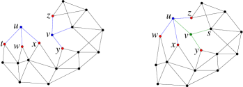
(a)                                  (b)

Figure 8: (a) Not a triangle net (b) A triangle net

Thus Fig. 8 (b) is an example of a triangle net. The graph shown in Fig. 8 (b), is generated from a triangle tree by adding extended nodes $u$ and then $v$. So $v$ is an apex of $G$. Triangle notch is a special case of triangle net.

Lemma 6

A triangle net is generically globally rigid.

Proof

See Appendix 0.A.4. ∎

3.3 Triangle bar

A graph $G$ is called a triangle bar, if it satisfies one of the followings:

1. $G$ can be obtained from a triangle cycle, triangle circuit, triangle bridge or triangle net by adding zero or more edges, but no extra node;

2. $G=B_{i}\cup B_{j}$ where $B_{i}$ and $B_{j}$ are triangle bars which share at least three nodes; or

3. $G=B_{i}\cup\{v\}$ where $B_{i}$ is a triangle bar and $v$ is a node not in $B_{i}$, and adjacent to at least three nodes of $B_{i}$.

Note that triangle cycle, triangle circuit, triangle bridge and triangle net are also triangle bars. These triangle bars will be referred as elementary bars.

Fig. 9 shows some examples of triangle bars. The first figure is a triangle cycle. Next two are triangle nets.

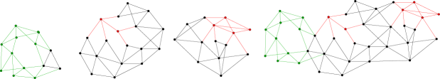
Figure 9: Examples of triangle bar

The fourth figure shows an example of a triangle bar which is obtained by stitching the first three elementary bars through common triangles.

Theorem 3.1

Triangle bar is generically globally rigid.

Proof

From Lemma 3 and 6, elementary bars are generically globally rigid. Suppose two triangle bars $B_{i}$ and $B_{j}$ share three nodes. Since all the nodes are in generic position, these three nodes are non-collinear. Using Lemma 1, $B_{i}\cup B_{j}$ is generically globally rigid.

Let a triangle bar $B$ be obtained from another triangle bar $B^{\prime}$ by adding a node $v$ which is adjacent to three nodes in $B^{\prime}$. In a generic realization of $B^{\prime}$, any node placed with three given distances from known positions has a unique location. So $B$ is generically globally rigid. ∎

Theorem 3.2

Trilateration graph and wheel extension are triangle bars.

Proof

See Appendix 3.2. ∎

4 Problem statement

A triangle bar is a class of graphs which includes trilateration and wheel extension graphs as special cases. Starting from a triangle of three reference nodes, we find a maximal triangle bar. Let $G({\cal T})$ be a triangle tree where ${\cal T}=(T_{1}$, $T_{2}$, $\ldots$, $T_{n})$. Three nodes in $T_{1}$ are chosen as the reference nodes. This triangle is called seed triangle. Our goal is to identify a maximal triangle bar containing $T_{1}$ and then mark the nodes in this triangle bar as localizable.

Problem 1

Consider a distance graph $G=(V,E,d)$, generically embedded in plane with a seed triangle $T_{1}$. Find a maximal triangle bar containing $T_{1}$ in a distributed environment and mark the nodes of the triangle bar as localizable.

We solve the problem involving only connectivity information. No distance information is used. Here onwards, we ignore the distance function $d$ and consider the graph $G=(V,E)$. The stated problem is solved by exploiting flips of triangles in $G$. In order to solve the problem, we introduce the notion of flip-triangle graph of $G$.

4.1 Flip-triangle graph

Given a graph $G=(V,E)$, we construct a graph ${\cal G}=({\cal V},{\cal E})$ with ${\cal V}$ = $\{t_{1}$, $t_{2}$, $\ldots$, $t_{N}\}$ where $t_{i}$ represents a triangle $T_{i}$ in $G$ and $\{t_{i},t_{j}\}\in{\cal E}$ if and only if $T_{i}$ and $T_{j}$ share an edge in $G$. The graph ${\cal G}$ is termed as flip-triangle graph of $G$, in short $FTG(G)$. If no ambiguity occurs, we use $t_{i}$ to denote a vertex of $FTG(G)$ and $T_{i}$ to refer the corresponding triangle in $G$. A maximal tree in $FTG(G)$ is called a flip-triangle tree ($FTT$). A connected $FTG(G)$ has unique $FTT$. Let ${\cal T}$ = $(T_{1}$, $T_{2}$, $\ldots$, $T_{m})$ be a sequence of triangles in $G$ and $\tau$ = $(t_{1}$, $t_{2}$, $\ldots$, $t_{m})$ be the corresponding sequence of nodes in ${\cal G}$. If no ambiguity occurs, ${\cal T}$ also means the subgraph obtained from the union of $T_{i}$s in ${\cal T}$. Similarly, $\tau$ means corresponding subgraph in ${\cal G}$. We describe some properties which are useful for developing the proposed algorithm.

Proposition 1

${\cal T}$ is a triangle cycle of length $n$ in $G$ if and only if $\tau$ is an $n$-cycle in ${\cal G}$.

Proof

Let ${\cal T}$ be a triangle cycle in $G$. By construction, pairs of nodes $t_{i}$ and $t_{i+1}$ for $1\leq i\leq n-1$, and $t_{m}$ and $t_{1}$ are adjacent in ${\cal G}$. For some $i$, $j$ $(|i-j|>1)$ (except $t_{1}$ and $t_{m}$), if $t_{i}$ and $t_{j}$ are adjacent in ${\cal G}$ then $T_{i}$ and $T_{j}$ share an edge. This contradicts that ${\cal T}$ is a triangle cycle in $G$. Therefore, $\tau$ is an $n$-cycle in ${\cal G}$.

Conversely, let $\tau$ be an $n$-cycle in ${\cal G}$. For some $i$, $j$ $(|i-j|>1)$ (except $T_{1}$ and $T_{m}$), if $T_{i}$ and $T_{j}$ share an edge in $G$ then $t_{i}$ and $t_{j}$ are adjacent in ${\cal G}$. It contradicts that $\tau$ is an $n$-cycle in ${\cal G}$. Therefore, ${\cal T}$ is a triangle cycle in $G$ of length $n$. ∎

Proposition 2

${\cal T}$ is a triangle tree in $G$ if and only if $\tau$ is a tree in ${\cal G}$.

Proof

Let ${\cal T}$ be a triangle tree in $G$. By construction, $\tau$ is connected subgraph in ${\cal G}$. In view of Proposition 1, $\tau$ contains a cycle in ${\cal G}$ if and only if ${\cal T}$ contains a triangle tree in $G$. Hence the result follows. ∎

Proposition 3

${\cal T}$ is a maximal triangle tree in $G$ if and only if $\tau$ is an $FTT$ in $FTG(G)$.

Proof

Let ${\cal T}$ be a maximal triangle tree in $G$. $\tau$ is a tree in ${\cal G}$ (Proposition 2). If $\tau$ is not an $FTT$ in $FTG(G)$, there exists a tree $\tau^{\prime}$ containing $\tau$ as a proper subtree in ${\cal G}$. The triangle tree ${\cal T}^{\prime}$ corresponding to $\tau^{\prime}$ also contains ${\cal T}$ as a proper subgraph in $G$. This is contradicts that ${\cal T}$ is a maximal triangle tree in $G$.

Conversely, let $\tau$ is an $FTT$. If ${\cal T}$ is not maximal triangle tree in $G$, there is a ${\cal T}^{\prime}$ containing ${\cal T}$ as a proper subgraph. ${\cal T}^{\prime}$ corresponds a tree $\tau^{\prime}$ in ${\cal G}$ (Proposition 2) while $\tau^{\prime}$ contains $\tau$ as a proper subtree. This is a contradiction. Hence the result follows. ∎

4.2 Solution plan

Consider a graph $G=(V,E)$. A triangle bar may be identified in $G$ by three rules as in its definition. First, we find elementary bars in $G$. If possible, then we stitch them via three common nodes to form a larger triangle bar; or extend a triangle bar ${\cal B}$ successively by adding a new node which is adjacent to at least three nodes of ${\cal B}$. After computing the $FTG(G)$, the stated problem is solved in a distributed set up as follows:

1. We identify all the components of ${\cal G}$. For each component ${\cal G}^{\prime}$ in ${\cal G}$, we compute a corresponding spanning tree $FTT({\cal G}^{\prime})$ which is a maximal subtree in ${\cal G}$.

2. Finding triangle cycles is equivalent to finding the cycles in ${\cal G}=FTG(G)$ (Proposition 1). We identify a set of base cycles (a minimal set of cycles such that any cycle of the graph may be obtained by union of some base cycles and deleting some parts).

3. A triangle chain is also a triangle tree. The generator chains of triangle circuits and bridges and generator trees of triangle nets are uniquely identified by subtrees in $FTG(G)$ (Proposition 2). We identify other elementary bars in $G$ from the $FTT$s by suitable extensions.

4. Finally, we stitch or extend these elementary bars to form a maximal triangle bar in $G$ containing $T_{1}$; then we mark the nodes in this triangle bar as localizable.

5 Localizability testing

This section describes a distributed technique to find the maximal triangle bar with a seed triangle $T_{1}$ in three phases. This triangle bar is reported as the localizable subgraph of $G$.

5.1 Representation of graph and flip-triangle graph

Each node contains data structures suitable for describing and storing necessary information for the execution of the algorithm. We assume that each node contains a unique number as its identification (called node-id) and a list (${\tt nbrs}$) of node-ids of its neighbours. The node contains no edge distance information. To represent a triangle in computer, we define a data structure, with type name ${\tt\mathbf{Trngl}}$, containing:   1) node-ids of the nodes of the triangle; and   2) a list of adjacent nodes in $FTG(G)$ (i.e., triangles sharing its edge in $G$). In a distributed environment, the node with minimum node-id among three nodes of a triangle is designated as the leader. The leader contains all the information of the triangle and processes them. Each node $v$ additionally contains a list (${\tt trngls}$) of all the triangles containing $v$ as the leader.

5.2 Communication protocols for $G$ and $FTG(G)$

A communication between two adjacent nodes in $FTG(G)$ (i.e., two triangles sharing an edge in $G$) means communication between their leaders which may involve at most 2-hop communication in $G$. Intermediate communications via other nodes uses standard communication tools for $G$ (i.e., communication within $G$). By a communication between a node $s_{i}\in G$ and a node $t_{j}\in FTG(G)$ (i.e., triangle $T_{j}$), we mean the communication between $s_{i}$ and the leader of $T_{j}$. The nodes of $G$ and $FTG(G)$ use different types of signals to indicate the types of the contents of the messages. We list these signals as follows:

Signal types	Significance of the symbol
visit	On arrival of this signal a node of $FTG(G)$ wake up and starts processing.
visitNode	On arrival of this signal a node of $G$ wake up and starts processing.
child	A node in $G$ sends a child signal to its parent to register itself as a child in parent.
cycle	A node in $G$ or $FTG(G)$ sends a cycle signal on identification of an elementary bar.

5.3 Phase I: Computing the $FTG$

Phase-I of the algorithm sets up the basic structure of the $FTG(G)$ using the procedures recvNbrList( ) and recvTriangle( ) described with pseudo-codes as follows.

1:procedure recvNbrList( ) /* $s_{i}$ = current node */

2:     Wake on arrival of neighbours (${\tt nbrs_{j}}$) form $s_{j}$

3:     for (each common $s_{k}$ in ${\tt nbrs_{j}}$ and ${\tt nbrs_{i}}$) do/* A triangle $T(\triangle s_{i}s_{j}s_{k})$ is identified. */

4:         if ($s_{i}$ is the leader of $T$) then /* $T$ corresponds new node in $FTG(G)$ */

5:              for (each $T^{\prime}\in s_{i}.{\tt trngls}$ sharing an edge with $T$) do /* Found a new edge $TT^{\prime}$ */

6:                  Push $T^{\prime}$ into $T.{\tt trngls}$ and $T$ into $T^{\prime}.{\tt trngls}$ as a neighbour of each other in ${\cal G}$.

7:                 /* Both of these push operations occur in $s_{i}$, since $s_{i}$ is the leader $T$ and $T^{\prime}$. */

8:              end for

9:              Store the new triangle $T$ into $s_{i}.{\tt trngls}$ in its leader.

10:              Send the triangle $T$ to $s_{j}$ and $s_{k}$ to find and set edges with other triangles.

11:         end if

12:     end for

13:end procedure

 

1:procedure recvTriangle( )/* $s_{i}$ = current node */

2:     Wake on arrival of a triangle $T(\triangle s_{j}s_{k}s_{l})$ such that $j<k<l$

3:     for (each $T^{\prime}\in s_{i}.{\tt trngls}$ sharing an edge with $T$) do /* Found a new edge $TT^{\prime}$ for ${\cal G}$ */

4:         Push $T$ into $T^{\prime}.{\tt trngls}$ as a neighbour of $T^{\prime}$ in $FTG(G)$. /* $s_{i}$ is the leader of $T^{\prime}$ */

5:     end for

6:     if ($i\in\{j,k,l\}$, say $i=l$) /* Note that beyond $1$-hop, $i\notin\{j,k,l\}$ */

7:         Send the triangle $T$ to all neighbours of the current node except $s_{j}$ and $s_{k}$

8:end procedure

Proposition 4

1. All the processes in Phase I are synchronized.

2. The algorithm guarantees the progress and finite termination of Phase I.

3. Number of communications from each node is thrice the number of neighbours.

4. Phase I of the algorithm computes the $FTG(G)$.

Proof

On arrival of a triangle message $T$, recvTriangle( ) wakes up. If the node is the leader of $T$, it stores the triangle information. It also checks, if $T$ shares an edge with the existing triangles in the list ${\tt trngls}$. Note that each triangle in the list ${\tt trngls}$ share an edge with $T$. We call these triangles as neighbour triangles of $T$.

Synchonization: Each node starts by sending its neighbour list (${\tt nbrs}$) to every neighbour. When a node $s_{i}$ receives the neighbour list from a node $s_{j}$, it identifies all triangles which contain $s_{i}$ and $s_{j}$ as two nodes. Each of two processes in Phase I is atomic. Any order of insertions of triangles into the neighbour triangle list will finally give the same result.

Progress and finite termination: Every node executes recvNbrList( ) exactly one for a neighbour list each neighbour. Each For loop runs over neighbour lists which are finite in size. Since the processes are atomic and loops runs on finite neighbour list, progress is guaranteed. In recvTriangle( ), If block conditions are false beyond $1$-hop from $s_{i}$ and stops resending $T$. Assumed channels are reliable, every message reaches its destination in finite time. We use Lamport’s logical clock. In each node, the value of logical clock does not exceed thrice the number of neighbours; one neighbour list and two triangle messages from each neighbour. It also follows the number of communications from a node.

Computation of $FTG(G)$: Each node receives a neighbour list of a neighbour exactly once. Consider an arbitrary triangle $T(\triangle s_{i}s_{j}s_{k})$ in $G$ (Fig. 10) while $i<j<k$. Let $T$ is received by $s_{i}$, the leader node of $T$. recvNbrList( ) inserts $T$ into $s_{i}.{\tt trngls}$. No other node incorporates $T$, though $s_{j}$ and $s_{k}$ also identify $T$. It may be adjacent to the edges in $FTG(G)$ due to sharing its edges with other triangles.

Figure 10: Examples showing all possible triangle communications

The inner for loop in recvNbrList( ) sets up the edges which are obtained while $T$ shares an edge with the triangles whose leader is $s_{i}$. $s_{i}$ also sends a triangle message $T$ to $s_{j}$ and $s_{k}$ to find and set other edges with $T$ in $FTG(G)$. $T$ shares no edge in $G$ beyond $1$-hop. The edges in $FTG(G)$ between $T$ and other triangles with leaders other than $s_{i}$ are set by recvTriangle( ). When $s_{j}$ (or $s_{k}$) receives $T$, it checks whether $T$ shares any triangle in its list ${\tt trngls}$ sends to sends $T$ to its neighbours other than $s_{i}$ and $s_{j}$. Thus $T$ reaches all the nodes which contains a triangle that may share an edge with $T$. ∎

5.4 Phase II: Finding $FTT$s and elementary bars

For finding elementary bars, we may assume that $G$ is connected; otherwise, we proceed with the component containing the seed triangle $T_{1}$. Phase-II identifies the $FTT$ of ${\cal G}$ containing $t_{1}$(i.e., $T_{1}$ in $G$); then elementary bars. This process is triggered by $t_{1}$ in ${\cal G}$ sending a $\mathbf{visit}$ signal to its adjacent nodes in ${\cal G}$.

5.4.1 Representation of $FTT$s of $G$ and elementary bars:

For this purpose, each node in ${\cal G}$ (a triangle in $G$) contains additional five fields:

1. ${\tt status}$ (assumes 0 or visited, initially 0) is used to indicate the status regarding the processing of the node. After the required processing of a node, ${\tt status}$ is set to visited.

2. ${\tt elementLst}$ is a list of elementary bars in which this particular node (triangle) is a constituent part; initially it is empty.

3. ${\tt parent}$ contains the immediate ancestor of the triangle in a $FTT$ of $G$. The seed triangle has no parent; and it is treated as root node.

4. ${\tt children}$ is a list containing direct descendants in ${\cal G}$. These are used to set the trees in ${\cal G}$.

5. ${\tt hearLst}$ holds the list of received triangles with some extra information that help in identifying elementary bars.

Each node in $G$ also contains similar five fields to store the information regarding pendants, extended knots and elementary bars.

5.4.2 Finding the $FTT$ and base cycles in ${\cal G}^{\prime}$:

The $FTT$ of ${\cal G}$ containing $T_{1}$ are identified by distributed $BFS$ on ${\cal G}$. If we take any $FTT$ and add to it a new edge from ${\cal E}$ a set of base cycles of ${\cal G}$ may be obtained. The details of these steps are described in procedure visitTriangle( ).

On arrival of $\mathbf{visit}$ signal into $t_{i}\in{\cal V}$, visitTriangle( ) in leader node of $T_{i}$ sets its status to $\mathbf{visited}$. $t_{i}.{\tt parent}$ is assigned the value $t_{j}$. This helps in backtracking in the tree in $FTG(G)$. After visiting $t_{i}$, the process sends $\mathbf{visit}$ signal to all neighbours in $FTG(G)$. At the same time, $t_{i}$ sends a $\mathbf{visitNode}$ signal with $T_{i}$ to the pendant $s_{k}$ of $T_{i}$ with respect to $T_{j}$ in $G$ for finding elementary bars other than triangle cycles.

1:procedure visitTriangle( ) /* $t_{i}$= current node of ${\cal G}^{\prime}$ */

2:     Wake on a $\mathbf{visit}$ signal from $t_{j}\in{\cal V}$

3:     if (${\tt status}\neq\mathbf{visited}$) then

4:         Set ${\tt parent}\leftarrow t_{j}$, ${\tt status}\leftarrow\mathbf{visited}$

5:         Send a $\mathbf{visit}$ signal to all adjacent nodes in ${\cal G}^{\prime}$ other than $t_{j}$

6:         Send a $\mathbf{child}$ signal to $t_{j}$ to indicate that $s_{i}$ is a child of $s_{j}$

7:         Send a $\mathbf{visitNode}$ signal to $s_{k}\in T_{i}-T_{j}$ with $T_{i}$ qualified as $\mathbf{triangle}$

8:     else/* a base cycle is identified by $t_{i}t_{j}$ */

9:         Push $T_{i}T_{j}$ into ${\tt elementLst}$ to indicate that $t_{i}$ lies in the cycle $T_{i}T_{j}$

10:         Send a $\mathbf{cycle}$ signal to $t_{j}$ and ${\tt parent}$ with $T_{i}T_{j}$ as elementary bar-id

11:     end if

12:end procedure

 

1:procedure elementaryBars($x_{i}$) /* $x_{i}$ is the current ($t_{i}\in{\cal V}$ or $s_{i}\in V$) */

2:     Wake on arrival of a $\mathbf{cycle}$ signal with elementary bar identity as $bar$-$id$

3:     if ($bar$-$id$ is qualified as $\mathbf{delete}$) then

4:         Delete $bar$-$id$ from ${\tt elementLst}$

5:     else if ($bar$-$id\notin{\tt elementLst}$) then

6:         Push $bar$-$id$ into ${\tt elementLst}$

7:         Send a $\mathbf{cycle}$ signal to ${\tt parent}$ with $bar$-$id$

8:     else/* Elementary bars in ${\cal G}^{\prime}$ are traced */

9:         Send a $\mathbf{cycle}$ signal with $bar$-$id$ qualified as $\mathbf{delete}$ to its ${\tt parent}$

10:     end if

11:end procedure

1:procedure visitNode( ) /* $s_{i}$=current node in $G$ */

2:     Wake on a $\mathbf{visitNode}$ signal with $X_{j}$ ($=T_{j}$ or $s_{j}$)

3:     Push $X_{j}$ into ${\tt hearLst}$

4:     if (${\tt status}\neq\mathbf{visited}$) then

5:         Set ${\tt parent}\leftarrow X_{j}$,   ${\tt status}\leftarrow\mathbf{visited}$

6:         if ($X_{j}=T_{j}$)/* $s_{i}\in T_{j}$, let $T_{j}=\triangle s_{i}s_{k}s_{m}$ */

7:              Send a $\mathbf{visitNode}$ signal with $s_{i}$ to all $s_{m}\in{\tt nbrs}-\{s_{k},s_{l}\}$

8:         Send a $\mathbf{child}$ signal to ${\tt parent}$ to inform that $s_{i}$ is a child

9:     else if ($X_{j}=T_{j}$) then/* if ${\tt parent}=T_{k}$ */

10:         Send a $\mathbf{cycle}$ signal to $t_{j}$ and $t_{k}$ with $T_{j}s_{i}T_{k}$ as elementary bar-id

11:     else if ($X_{j}=s_{j}$) then

12:         if (${\tt parent}=T_{k}$) then /* a bridge or net */

13:              Send a $\mathbf{cycle}$ signal to $s_{j}$ and $t_{k}$ with $s_{j}s_{i}T_{k}$ as elementary bar-id

14:         else if (${\tt parent}=s_{k}$) then

15:              if (${\tt mark}=\textbf{extended}$) then

16:                  Send a $\mathbf{visitNode}$ signal with $s_{i}$ to all $s_{m}\in{\tt nbrs}-\{s_{k}\}$

17:                  Send a $\mathbf{cycle}$ signal to $s_{j}$ and $s_{k}$ with $s_{j}s_{i}s_{k}$ as elementary bar-id

18:              else if ($size({\tt hearLst})=3$) then

19:                  Set ${\tt mark}\leftarrow\mathbf{extended}$

20:                  for all ($s_{j}\in{\tt hearLst}$) do

21:                       Send a $\mathbf{cycle}$ signal to $s_{k}$ and $s_{j}$ with $s_{j}s_{i}s_{k}$ as bar-id

22:                  end for

23:              end if

24:         end if

25:     end if

26:end procedure

It sends back a $\mathbf{child}$ signal to the sender $t_{j}$ to inform itself as a child. The $\mathbf{child}$ signal is handled (handler is not described separately) by inserting its sender into the list ${\tt children}$. If $t_{i}$ is already visited by some other node $t_{k}$, a base cycle in $FTG(G)$ is identified with $t_{i}t_{j}$ and sends a $\mathbf{cycle}$ signal with $t_{i}t_{j}$ to $t_{j}$ and $t_{k}$. A cycle in $FTG(G)$ corresponds a triangle cycle in $G$ (Proposition 1). A triangle cycle $G$, corresponding to a base cycle in $FTG(G)$, contains at least one new triangle which is not a part of any other triangle cycle in $G$. The outcome of the procedure may be summarized below in an proposition.

Proposition 5

visitTriangle( ) identifies the $FTT$ and triangle cycles of $G$ containing $T_{1}$.

5.4.3 Finding triangle circuits and triangle bridges in ${\cal G}^{\prime}$:

Triangle cycles are identified by handling $\mathbf{cycle}$ signals. In view of the Proposition 3, a $FTT$ generate maximal triangle tree in $G$. These maximal trees provide maximal triangle bars including appropriate edges and extended knots. The steps are described in the procedure visitNode( ).

On arrival of a $\mathbf{visitNode}$ signal with $X_{j}$ (either a triangle $T_{j}$ or a node $s_{j}$), a node $s_{i}\in V$ wakes up and visitNode( ) stores $X_{j}$s into a list ${\tt hearLst}$. If $s_{i}$ is being visited for the first time as a node in $G$, $s_{i}$ set its ${\tt status}$ as visited and ${\tt parent}$ to $X_{j}$ for backtracking. If $X_{j}=T_{j}$ and $s_{i}$ is a pendant of $T_{j}$, $s_{i}$ sends a $\mathbf{visitNode}$ signal with $s_{i}$ to all neighbours other those in $T_{j}$. Otherwise, if $s_{i}$ 1) receives a triangle $T_{j}$ and its parent is a triangle $T_{k}$, a triangle circuit is identified; 2) receives a node $s_{j}$ and its parent is a triangle $T_{k}$ (either a pendant or extended knot), a triangle bridge or net is identified; and 3) if three $\mathbf{visitNode}$ signals, it identifies itself as an extended knot and as well as a triangle net. If $s_{i}$ marks himself as an extended knot it sends $\mathbf{visitNode}$ signal with $s_{i}$ to all neighbours except its parent for identifying other extended knots and nets. Note that $\mathbf{visitNode}$ signal with triangle is sent only to a pendant from the process visitTriangle( ). The final outcome of this process is described below.

Proposition 6

All triangle circuits and triangle bridges in ${\cal G}^{\prime}$ are identified by visitNode( ).

5.4.4 Identifying triangle nets in ${\cal G}^{\prime}$:

On arrival of a $\mathbf{cycle}$ signal into $x_{i}$ (either a node in $FTG(G)$ or pendant or extended knots in $G$), elementaryBars( ) inserts elementary bar-id into the ${\tt elementLst}$ and in turn sends the same $\mathbf{cycle}$ signal to its parent until it finds a node in $FTG(G)$ containing same elementary bar-id in respective ${\tt elementLst}$. If a matching bar-id is found, it sends $\mathbf{cycle}$ signal with this bar-id qualified as $\mathbf{delete}$. If it finds bar-id qualified as $\mathbf{delete}$ and bar-id is deleted from ${\tt elementLst}$ and sends $\mathbf{delete}$ signal same bar-id qualified as $\mathbf{delete}$ to its parent until the root node $t_{1}$ in $FTG(G)$ is reached.

5.5 Phase III: Identifying the maximal triangle bar containing $T_{1}$

visitNode( ) and elementaryBars( ) provide a maximal triangle bar for the $FTT$. Thus, we have obtained a set ${\cal M}$ of maximal triangle bars for the $FTT$ containing $T_{1}$. Maximal triangle bars for a $FTT$ do not share any triangle in this $FTT$. From ${\cal M}$, two maximal triangle bars $M_{1}$ and $M_{2}$ which have three nodes in common are replaced by $M_{1}\cup M_{2}$. Repeat these until no replacement. This task may be achieved by sending a special signal from all nodes of $M_{1}$ (assuming that $M_{1}$ contains $T_{1}$) to their neighbours. Another $M_{i}$ sends this special signal if it hears this signal from three nodes. Finally, a maximal triangle bar in $G$ will be identified.

Proposition 7

The maximal triangle bar of $G$ containing $T_{1}$ is identified in polynomial time with $O(|E|)$ one-hop communications over the network.

Mark localizable nodes:

At the end of Phase-II when $t_{1}.{\tt elementLst}$ is empty, $t_{1}$ set its ${\tt status}$ as $\mathbf{localizable}$. The triangle $T_{1}$ (i.e., $t_{1}$) triggers the Phase-III by sending the ${\tt elementLst}$ to all its adjacent nodes (${\tt children}$) in ${\cal G}$. On arrival of an elementary bar list into $x_{i}$ ($t_{i}\in FTG(G)$ or $s_{i}\in G$), markLocalizable( ) starts execution.

1:procedure markLocalizable($x_{i}$) /* $x_{i}$ is the current ($t_{i}\in{\cal V}$ or $s_{i}\in V$) */

2:     Wake on arrival of an elementary bar list, say $barLst$

3:     if ($barLst\cap{\tt elementLst}\neq\emptyset$ and ${\tt status}\neq\mathbf{localizable}$) then

4:         Set ${\tt status}\leftarrow\mathbf{localizable}$

5:         Send a message with ${\tt elementLst}$ to all nodes in $x_{i}.{\tt children}$

6:     end if

7:end procedure

If the current node, $x_{i}$, lies in an elementary bar in the received list and is not marked as localizable, the process marks $x_{i}$ as localizable and sends $x_{i}.{\tt elementLst}$ to all nodes in $x_{i}.{\tt children}$.

Theorem 5.1

If an elementary bar contains $T_{1}$, then all the nodes (in $G$) of these bars are marked as localizable through markLocalizable( ) (identifying the bar through $T_{1}$) in the complete run of the algorithm.

Proof

The result follows from the statements in Proposition 1, 2, 5 6. ∎

6 Performance analysis of the algorithm

6.0.1 Synchronization, Correctness and Progress:

Phase I computes the $FTG(G)$. Its synchronization, progress, finite termination and correctness of are proved in Proposition 4. Phase II uses $BFS$ tool to find the trees in a connected $FTG(G)$. This ensures that the $FTT$s are found correctly (Proposition 3). Theorems 3.1 and 5.1 establish the correctness of Phase II and III of the algorithm.

Each of the procedures in the algorithm may contain loop which run over a list either ${\tt nbrs}$ or ${\tt trngls}$. The sizes of these lists do not exceed the number of neighbours of a node. The loops executes without waiting for any signal. Therefore, the finite termination of each procedure in any individual node is guaranteed. Since the transmission medium is reliable, every message sometime reaches the destination. Thus, executions in the whole system terminate in finite time.

6.0.2 Time complexity:

We have used Lamport’s logical clock. The maximum value of this logical clock in any node does not exceed thrice the number of its neighbours (Proposition 4). Phase I communicates no message beyond $2$-hop. The running time complexity of recvNbrList( ) in each node is $O(n)$ in the worst case. Therefore, the worst case time complexity of Phase I is $O(n^{2})$ in total. Time complexity for communication in Phase II and III is guided by the $BFS$ of $FTG(G)$ in distributed way. A visit signal from $t_{1}$ will reach any other $t_{i}$ in $FTG(G)$ along its shortest path in between them. In worst case, it may be equal $|V|$. This dominates time required to find extended knots. Thus, the worst case time complexity is equal to the number of nodes in $G$, i.e., $O(n)$. Thus the overall time complexity of the execution in the whole system is $O(n^{2})$.

6.0.3 Energy complexity:

Since message communication dominates the leading consumer of energy, we only count the communications for energy analysis. Every node sends the neighbour list ${\tt nbrs}$ only once. It counts $n$ (number of nodes in the network) transmissions. A node executes recvNbrList( ) once for each of its neighbours. recvNbrList( ) sends a triangle message for a newly obtained triangle whose leader is a different. The total number of these triangle messages is $|E|$ maximum. recvNbrList( ) also sends a flip message for a newly obtained flip with a triangle whose leader is a different node. The total number of such flip messages does not exceed $|E|$. Thus the number message transmissions in Phase I is $O(|E|)$. It is easy to see that, in Phase II and Phase III, each node communicates with its neighbours constant number of times. Hence, the total energy dissipation is $O(|E|)$ in worst.

7 Conclusion

In this paper, we consider the problem of localizability of nodes as well as networks. We do not compute the positions of nodes. So, exact distances are not necessary and error in distance measurements does not affect the localizability testing. We propose an efficient distributed technique to solve this problem for a specific class of networks, triangle bar. The proposed technique is better than both trilateration and wheel extension techniques. We also illustrate some network scenarios which are wrongly reported as not localizable by wheel extension technique, but the proposed algorithm recognizes them as localizable in a distributed environment. The proposed algorithm runs with $O(|V|^{3})$ time complexity and energy complexity of $O(|E|)$ in the worst case.

In centralized environment localizability testing can be carried out in polynomial time. Though the proposed algorithm recognizes a class of localizable networks distributedly, several localizable networks remains unrecognized by this technique. For localizability testing, we only consider a maximal triangle bar of $G$ which includes the anchor triangle $T_{1}$ in $G=(V,E,d)$. Our future plan is to extend localizability testing considering other triangle bars in $FTG(G)$.

Appendix 0.A Appendix

0.A.1 Proof of the first part of Lemma 2

Proof

A wheel graph $W_{n}$ with $n$ nodes is a triangle cycle with $n-1$ triangles. A triangle cycle with three or four triangles is a wheel $W_{4}$ or a wheel $W_{5}$ (Fig. 12) respectively. These wheels show the existence of spanning wheels for some triangle cycles. Consider a sufficiently large triangle cycle $G({\cal T})$ with the triangle stream ${\cal T}=(T_{1},T_{2},\ldots,T_{n})$ which has no spanning wheel. If we consider three consecutive triangles in ${\cal T}$, then we have at least one node with degree at least four. Consider such a node $v$ with $deg(v)\geq 4$. If $deg(v)=4$, then the edges incident on $v$ lie in three consecutive triangles $T_{i}$, $T_{i+1}$, $T_{i+2}$ (Fig. 12 (a)).

Figure 11: Triangle cycle with three and four triangles

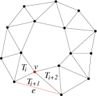
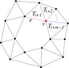
(a)                                    (b)

Figure 12: Triangle cycles without spanning wheel

Deleting the outer side $e$ of $T_{i+1}$ (i.e., $G({\cal T})-e$) gives a spanning triangle circuit of $G({\cal T})$. Suppose, $deg(v)=m>4$. The edges adjacent to $v$ lie in $m-1$ consecutive triangles $T_{i+1}$, $T_{i+2}$, $\ldots$, $T_{i+m-1}$ (Fig. 12 (b)). Deleting the outer side of $T_{i+1}$ gives a spanning triangle circuit of $G({\cal T})$. ∎

0.A.2 Proof of the second part of Lemma 2

Proof

Let $G({\cal T})$ be a triangle circuit with triangle stream ${\cal T}=(T_{1}$, $T_{2}$, $\ldots$, $T_{n})$ and circuit knot $v$ (Fig. 13). $v$ is the only pendant for both $T_{1}$ and $T_{n}$. $T_{2}$ and $T_{3}$ share the edge $f$ and $w$ is the corresponding pendant in $T_{2}$.

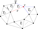
Figure 13: Triangle circuit ${\cal T}$ gives a spanning triangle bridge ${\cal T}-e$

$T_{1}$ has two outer sides which are incident on $v$; one edge is incident on $w$ and the other is incident on $f$. If $e$ is the outer side of $T_{1}$ incident on $f$, then $G({\cal T})-e$ gives a spanning triangle bridge of $G({\cal T})$. ∎

0.A.3 Proof of Lemma 4

Proof

Let $G$ be a triangle notch generated from a triangle tree $G({\cal T})$ with the apex $v$. $G$ contains $n+2$ nodes $u_{i}$, $i=1$, $2$, $\ldots$, $n+2$. All the leaf knots of $G({\cal T})$ are adjacent to $v$. Fig. 6 (b) shows an example of such a graph. The leaf knots $u_{i}$, $u_{j}$ and $u_{k}$ of $G({\cal T})$ are adjacent to $v$. Consider a generic configuration $\cal P$ of $G$ where $v$ is realized as $(x,y)$ and $u_{i}$ as $(x_{i},y_{i})$ for $i=1$, $2$, $\ldots$, $n+2$. $G({\cal T})$ can have only flips. If possible, let a flip operation on $\cal P$ generate a different configuration ${\cal P}^{\prime}$ with coordinates $(x^{\prime},y^{\prime})$ for $v$ and $(x_{i}^{\prime},y_{i}^{\prime})$ for $u_{i}$, $i=1$, $2$, $\ldots$, $n+2$. Without loss of generality, we assume that the leaf triangle $T_{i}$, with a leaf knot $u_{i}$, remains fixed in both the configurations $\cal P$ and ${\cal P}^{\prime}$. Consider another leaf triangle $T_{j}$ with leaf knot $u_{j}$. Let ${\cal T}_{ij}$ be the unique triangle stream from $T_{i}$ to $T_{j}$ in the graph $G({\cal T})$. Proceeding in a manner similar to that in the proof of Lemma 3, each of $x_{j}^{\prime}$ and $y_{j}^{\prime}$ can be expressed in the form of $\frac{\phi}{\psi}$ where $\phi$ and $\psi$ are two non-zero polynomials of the coordinates of the points in ${\cal T}_{ij}-\{u_{i}\}$ with integer coefficients such that $\psi\neq 0$. From elementary coordinate geometry in $\mathbb{R}^{2}$, $x^{\prime}$ and $y^{\prime}$ can also be expressed similarly in terms of the coordinates of the points in ${\cal T}_{ij}$. Similarly, from the triangle stream ${\cal T}_{jk}$, $x_{k}^{\prime}$ and $y_{k}^{\prime}$ have similar expressions involving the coordinates of the points in ${\cal T}_{jk}-\{u_{i},v\}$. Since, the edge distance between $u_{k}$ and $v$ is given, then at least the coordinates of $u_{i}$, $v$ and $u_{k}$ are algebraically dependent. This contradicts the assumption that every three nodes in $\cal P$ are in general position. So the union of ${\cal T}_{ij}$, ${\cal T}_{jk}$ and $v$ in $\cal P$ admits no flip; and the union is generically globally rigid. Since, the leaf triangles chosen are arbitrary and any triangle lies on at least one triangle stream between some pair of leaf triangles, the generic global rigidity of $G$ follows. ∎

0.A.4 Proof of Lemma 6

Proof

Consider a triangle net $G$ generated by a triangle tree $G({\cal T})$ where ${\cal T}=(T_{1},T_{2},\ldots,T_{n})$. If $u_{r}$ is an apex of $G$, then the extended nodes have an ordering $u_{1}$, $u_{2}$, $\ldots$, $u_{r}$. Consider a generic configuration of $G$ (e.g. Fig. 14).

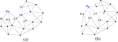
Figure 14: Triangle nets with extended nodes $u$ and $v$ where (a) $u$, $v$ are adjacent to pendants only, (b) $u$, $v$ are adjacent to both pendant and extended nodes

The extended node added to $G({\cal T})$ is $u_{1}$ which is adjacent to only pendants. These pendants are leaf knots of a triangle tree, which is a subgraph of $G({\cal T})$. This triangle tree is a triangle notch; hence it is generically globally rigid (Lemma 4).

Consider a leaf knot $y$ (e.g., Fig. 14). Let $P$ be an extending path which connects $y$ to the apex $u_{r}$. In view of Lemma 5, considering the extended nodes along $P$ and combining the corresponding generically globally rigid graphs, $G$ is generically globally rigid. ∎

0.A.5 Proof of Theorem 3.2

Proof

Let $G$ be a trilateration graph having a trilateration ordering $\pi=(u_{1},u_{2},\ldots,u_{n})$ where $u_{1}$, $u_{2}$ and $u_{3}$ are in $K_{3}$. $u_{4}$ is adjacent to three nodes before $u_{4}$ in $\pi$. So $u_{1}$, $u_{2}$, $u_{3}$ and $u_{4}$ form a $K_{4}$ which is a triangle cycle and consequently a triangle bar. Suppose $\pi^{\prime}=(u_{1},u_{2},\ldots,u_{i})$, $4\leq i<n$ forms a triangle bar ${\cal B}^{\prime}$. The node $u_{i+1}$ is adjacent to at least three nodes in ${\cal B}^{\prime}$. Therefore, ${\cal B}^{\prime}\cup\{v_{i+1}\}$ is a triangle bar. By mathematical induction, $G$ is a triangle bar.

Consider a wheel extension graph $G$ with a node ordering $\pi=(u_{1}$, $u_{2}$, $\ldots$, $u_{n})$. $u_{1}$, $u_{2}$ and $u_{3}$ are in $K_{3}$ and $u_{i}$ ($i\geq 4$) lies in a wheel containing at least three nodes in $\pi$ before $u_{i}$. So, $u_{4}$ lies on a wheel, say $W_{1}$, which contains $u_{1}$, $u_{2}$ and $u_{3}$. If any, let $u_{j}$, $j>4$, be the first node in $\pi$ such that $u_{j}$ does not lie on $W_{1}$. $u_{j}$ lies on another wheel, say $W_{2}$, which shares at least three nodes with $W_{1}$. Therefore, $W_{1}\cup W_{2}$ is generically globally rigid (by Lemma 1). Similarly, let $u_{k}$, if any, be the first node in $\pi$ such that $u_{k}$ does not lie on $W_{1}\cup W_{2}$. Assume $u_{k}$ lies on a wheel $W_{3}$ which shares three nodes with $W_{1}\cup W_{2}$. By Lemma 1, $W_{1}\cup W_{2}\cup W_{3}$ is generically globally rigid. Proceeding in this way, we can obtain, ${\cal W}=(W_{1},W_{2},\ldots,W_{m})$, a finite sequence of wheels such that each $W_{i}$ shares at least three nodes on some $W_{j}$s before $W_{i}$ in ${\cal W}$ and $G=\bigcup\limits_{i=1}^{m}W_{i}$, $m\geq 1$. Wheel graph is triangle cycle. Hence, $G$ is a triangle bar. ∎

References

- [1] Laman, G.: On graphs and rigidity of plane skeletal structures. Journal of Engineering Mathematics 4(4) (December 1970)
- [2] Hendrickson, B.: Conditions for unique graph realizations. SIAM J. Comput 21 (1992) 65–84
- [3] apkun, S., Hamdi, M., Hubaux, J.P.: Gps-free positioning in mobile ad hoc networks. Cluster Computing 5 (2002) 157–167
- [4] Aspnes, J., Eren, T., Goldenberg, D., Morse, A., Whiteley, W., Yang, Y., Anderson, B., Belhumeur, P.: A theory of network localization. Mobile Computing, IEEE Transactions on 5(12) (December 2006) 1663–1678
- [5] Connelly, R.: Generic global rigidity. Discrete and Computational Geometry 33(4) (2005) 549–563
- [6] Moore, D., Leonard, J., Rus, D., Teller, S.: Robust distributed network localization with noisy range measurements. In: SenSys ’04: Proceedings of the 2nd international conference on Embedded networked sensor systems, New York, NY, USA, ACM (2004) 50–61
- [7] Biswas, P., Toh, K.C., Ye, Y.: A distributed sdp approach for large-scale noisy anchor-free graph realization with applications to molecular conformation. SIAM J. Sci. Comput. 30(3) (2008) 1251–1277
- [8] Cakiroglu, A., Erten, C.: Fully decentralized and collaborative multilateration primitives for uniquely localizing wsns. EURASIP Journal on Wireless Communications and Networking 2010, Article ID 605658, 7 pages (2010)
- [9] Kwon, O.H., Song, H.J., Park, S.: Anchor-free localization though flip error resistant map stitching in wireless sensor network. IEEE Transactions on Parallel and Distributed Systems 99(PrePrints) (2010)
- [10] Zhu, Z., So, A.C., Ye, Y.: Universal rigidity: Towards accurate and efficient localization of wireless networks. In: IEEE INFOCOM 2010. (2010)
- [11] Saxe, J.: Embeddability of weighted graphs in -space is strongly np-hard. In: Proc. 17th. Allerton Conference in Communications, Control and Computing. (1979) 480–489
- [12] Jackson, B., Jordán, T.: Connected rigidity matroids and unique realizations of graphs. Journal of Combinatorial Theory Series B 94(1) (2005) 1–29
- [13] Yang, Z., Liu, Y., Li, X.: Beyond trilateration: on the localizability of wireless ad hoc networks. IEEE/ACM Trans. Netw. 18(6) (December 2010) 1806–1814
- [14] Niculescu, D., Nath, B.: Dv based positioning in ad hoc networks. Journal Telecommunication Systems 22 (2003) 267–280
- [15] Savvides, A., Han, C., Strivastava, M.: Dynamic fine-grained localization in ad-hoc networks of sensors. In: Proc. of the Annual International Conference on Mobile Computing and Networking (MobiCom 2001), Rome, Italy, ACM (July 2001) 166–179
- [16] Sau, B., Mukhopadhyaya, K.: Length-based anchor-free localization in a fully covered sensor network. In: Proc. of the First international conference on COMmunication Systems And NETworks. COMSNETS’09, Piscataway, NJ, USA, IEEE Press (2009) 137–146