Optimal Payoffs under State-dependent Preferences

Abstract

Most decision theories, including expected utility theory, rank dependent utility theory and cumulative prospect theory, assume that investors are only interested in the distribution of returns and not in the states of the economy in which income is received. Optimal payoffs have their lowest outcomes when the economy is in a downturn, and this feature is often at odds with the needs of many investors. We introduce a framework for portfolio selection within which state-dependent preferences can be accommodated. Specifically, we assume that investors care about the distribution of final wealth and its interaction with some benchmark. In this context, we are able to characterize optimal payoffs in explicit form. Furthermore, we extend the classical expected utility optimization problem of Merton to the state-dependent situation. Some applications in security design are discussed in detail and we also solve some stochastic extensions of the target probability optimization problem.

Key-words: Optimal portfolio selection, state-dependent preferences, conditional distribution, hedging, state-dependent constraints.

Introduction

Studies of optimal investment strategies are usually based on the optimization of an expected utility, a target probability or some other (increasing) law-invariant measure. Assuming that investors have law-invariant preferences is equivalent to supposing that they care only about the distribution of returns and not about the states of the economy in which the returns are received. This is, for example, the case under expected utility theory, Yaari’s dual theory, rank-dependent utility theory, mean-variance optimization and cumulative prospect theory. Clearly, an optimal strategy has some distribution of terminal wealth and must be the cheapest possible strategy that attains this distribution. Otherwise, it is possible to strictly improve the objective and to contradict its optimality. Dybvig (1988) was the first to study strategies that reach a given return distribution at lowest possible cost. Bernard and Boyle (2010) call these strategies cost-efficient and their properties have been examined further in Bernard, Boyle and Vanduffel (2014a). In a fairly general market setting these authors show that the cheapest way to generate a given distribution is obtained by a contract whose payoff is decreasing in the pricing kernel (see also Carlier and Dana (2011)). The basic intuition is that investors consume less in states of economic recession because it is more expensive to insure returns under these conditions. This feature is also explicit in a Black-Scholes framework, in which optimal payoffs at time horizon $T$ are shown to be an increasing function of the price of the risky asset (as a representation of the economy) at time $T$. In particular, such payoffs are path-independent.

An important issue with respect to the optimization criteria and the resulting payoffs under most standard frameworks, is that their worst outcomes are obtained when the market declines. Arguably, this property of optimal payoffs does not fit with the aspirations of investors, who may seek protection against declining markets or, more generally, may consider a benchmark when making investment decisions. In other words, two payoffs with the same distribution do not necessarily present the same “value” for a given investor. Bernard and Vanduffel (2014b) show that insurance contracts can usually be substituted by financial contracts that have the same payoff distribution but are cheaper. The existence of insurance contracts that provide protection against specific events shows that these instruments must present more value for an investor than financial payoffs that lack this feature. This observation supports the general observation that investors are more inclined to receive income in a “crisis” (for example when their property burns down or when the economy is in recession) than under “normal” conditions.

This paper makes several theoretical contributions to the study of optimal investment strategies and highlights valuable applications of its findings in the areas of portfolio management and security design. First, we clarify the setting under which optimal investment strategies necessarily exhibit path-independence. These findings complement Cox and Leland (1982, 2000) and Dybvig’s (1988) seminal results and underscore the important role of path-independence in traditional optimal portfolio selection. Thereafter, as our main contribution, we introduce a framework for portfolio selection that makes it possible to consider the states in which income is received. More precisely, it is assumed that investors target some distribution for their terminal wealth and additionally aim for a certain (desired) interaction with a random benchmark. For example, the investor may want his strategy to be unrelated to the benchmark when it decreases but to follow this benchmark when it performs well. Using our framework, we can characterize optimal payoffs explicitly (Theorems 3.2 and 3.4) in this setting. Such explicit characterizations are derived independently in Theorems 3.1 and 3.3 of Takahashi and Yamamoto (2013) but proved only for cases in which there is a countable number of states. Furthermore, we show that optimal strategies in this setting become conditionally increasing functions of the terminal value of the underlying risky asset.

A further main contribution in this part of the paper is the extension of the classical result of portfolio optimization under expected utility (Cox and Huang (1989)). Specifically, we determine the optimal payoff for an expected utility maximizer under a dependence constraint, reflecting a desired interaction with the benchmark (Theorem 5.2). The proof builds on isotonic approximations and their properties (Barlow et al. (1972)). We also solve two stochastic generalizations of Browne (1999) and Cvitanic̀ and Spivak’s (1999) classical target optimization problem in the given state-dependent context.

Finally, we show how these theoretical results are useful in security design and can help to simplify (and improve) payoffs commonly offered in the financial markets. We show how to substitute highly path-dependent products by payoffs that depend only on two underlying assets, which we refer to as “twins”. This result is illustrated with an extensive discussion of the optimality of Asian options. We also construct alternative payoffs with appealing properties.

The paper is organized as follows. Section 1 outlines the setting of the investment problem under study. In Section 2, we restate basic optimality results for path-independent payoffs for investors with law-invariant preferences. We also discuss in detail the sufficiency of path-independent payoffs when allocating wealth. In Section 3, we point out drawbacks of optimal path-independent payoffs and introduce the concept of state-dependence used in the following sections. We show that “twins”, defined as payoffs that depend only on two underlying asset values, are optimal for state-dependent preferences. In Section 4, we discuss applications to improve security designs. In particular, we propose several improvements in the design of geometric Asian options. In Section 5, we solve the standard Merton problem of maximization of expected utility of final wealth when the investor constrains the interaction of the final wealth with a given benchmark. In this context, we also generalize the results of Browne (1999) and Cvitanic̀ and Spivak (1999) with regard to target probability maximization. Final remarks are presented in Section 6. Most of the proofs are provided in the Appendix.

1 Framework and notation

Consider investors with a given finite investment horizon $T$ and no intermediate consumption. We model the financial market on a filtered probability space $\left(\Omega,\mathcal{F},\mathbb{P}\right),$ in which $\mathbb{P}$ is the real-world probability measure. The market consists of a bank account $B$ paying a constant risk-free rate $r>0$, so that $B_{0}$ invested in a bank account at time $0$ yields $B_{t}=B_{0}e^{rt}$ at time $t.$ Furthermore, there is a risky asset (say, an investment in stock) whose price process is denoted by $S=\left(S_{t}\right)_{0\leqslant t\leqslant T}.$ We assume that $S_{t}$ $(0<t<T)$ has a continuous distribution $F_{S_{t}}$. The no-arbitrage price at time 0 of a payoff $X_{T}$ paid at time $T>0$ is given by

$$c_{0}(X_{T})=\mathbb{E}[\xi_{T}X_{T}],$$ (1)

where $(\xi_{t})_{t}$ is the state-price density process ensuring that $(\xi_{t}S_{t})_{t}$ is a martingale. Moreover, based on standard economic theory, we assume throughout this paper that state prices are decreasing with asset prices, i.e.,

$$\xi_{t}=g_{t}(S_{t}),\text{ }t\geqslant 0,$$ (2)

where $g_{t}$ is decreasing (in markets where $\mathbb{E}[S_{T}]>S_{0}e^{rT}$). There is empirical evidence that this relationship may not hold in practice, which is called the pricing kernel puzzle (Brown and Jackwerth (2004), Grith et al. (2013)). Many explanations have been provided in the literature (Brown and Jackwerth (2004), Hens and Reichlin (2013)), including state-dependence of preferences (Chabi-Yo et al. (2008)). Therefore, (2) is not consistent with a market populated by investors with state dependent preferences. However, we do not tackle the problem of equilibrium and instead study the situation of a small investor whose state-dependent preferences do not influence the pricing kernel that is exogenously given in the market. This is a commonly studied situation since the work of Karatzas et al. (1987).

The functional form (2) for $(\xi_{t})_{t}$ allows us to present our results regarding optimal portfolios using $(S_{t})_{t}$ as a reference, which is practical. We will explain in Section 6 how the results and characterizations of the optimality of a payoff $X_{T}$ are tied to its (conditional) anti-monotonicity with $\xi_{T}$ and do not depend on the functional form (2) per se. Note that assumption (2) is satisfied by many popular pricing models, including the CAPM, the consumption-based models and by exponential Lévy markets in which the market participants use Esscher pricing (Vanduffel et al. (2008), Von Hammerstein et al. (2014)). It is also possible to use a market model in which prices are obtained using the Growth Optimal portfolio (GOP) as numéraire (Platen and Heath (2006)), as is discussed further in Section 6.

The Black–Scholes model can be seen as a special case of this latter setting. Since we will use it to illustrate our theoretical results, we recall here its main properties. In the Black–Scholes market, under the real probability $\mathbb{P}$, the price process $\left(S_{t}\right)_{t}$ satisfies

$$\frac{dS_{t}}{S_{t}}=\mu dt+\sigma dZ_{t},$$

with solution $S_{t}=S_{0}\exp\left(\left(\mu-\frac{\sigma^{2}}{2}\right)t+\sigma Z_{t}\right)$. Here, $\left(Z_{t}\right)_{t}$ is a standard Brownian motion, $\mu$ ($>r$) the drift and $\sigma>0$ the volatility. The distribution (cdf) of $S_{T}$ is given as

$$F_{S_{T}}(x)=\mathbb{P}(S_{T}\leqslant x)=\Phi\left(\frac{\ln\left(\frac{x}{S_{0}}\right)-(\mu-\frac{\sigma^{2}}{2})T}{\sigma\sqrt{T}}\right),$$ (3)

where $\Phi$ is the cdf of a standard normal random variable. In the Black–Scholes market, the state-price density process $(\xi_{t})_{t}$ is unique and $\xi_{t}=e^{-rt}e^{-\theta Z_{t}-\frac{\theta^{2}t}{2}}$ where $\theta=\frac{\mu-r}{\sigma}$. Consequently, $\xi_{t}$ can also be expressed as a decreasing function of the stock price $S_{t}$,

$$\xi_{t}=\alpha_{t}\left(\frac{S_{t}}{S_{0}}\right)^{-\beta},$$ (4)

where $\alpha_{t}=\exp\left(\frac{\theta}{\sigma}\left(\mu-\frac{\sigma^{2}}{2}\right)t-\left(r+\frac{\theta^{2}}{2}\right)t\right),\ \beta=\frac{\theta}{\sigma}>0$ (because we assume that $\mathbb{E}[S_{T}]=S_{0}e^{\mu T}>S_{0}e^{rT}$).

2 Law-invariant preferences and optimality of path-independent payoffs

In this section, it is understood that investors have law-invariant (state-independent) preferences. This means that they are indifferent between two payoffs having the same payoff distribution (under $\mathbb{P}$). In this case, any random payoff $X_{T}$ (that possibly depends on the path of the underlying asset price) admits a path-independent alternative with the same price, which is at least as good for (i.e., desirable in the eyes of) these investors. Recall that a payoff is path-independent if there exists some function $f$ such that $X_{T}=f(S_{T})$ holds almost surely. Hence, investors with law-invariant preferences only need to consider path-independent payoffs when making investment decisions. Under the additional (typical) assumption that preferences are increasing, any path-dependent payoff can be strictly dominated by a path-independent one that is increasing in the risky asset.

Note that results in this section are related closely to the original work of Cox and Leland (1982, 2000), Dybvig (1988), Bernard, Boyle and Vanduffel (2014a) and Carlier and Dana (2011). These overview results are recalled here to facilitate the exposition of the extensions that are developed in the following sections.

2.1 Sufficiency of path-independent Payoffs

Proposition 2.1 shows that for any given payoff there exists a path-independent alternative with the same price that is at least as good for investors with law-invariant preferences. Thus, such an investor needs only to consider path-independent payoffs. All other payoffs are indeed redundant in the sense that they are not needed to optimize the investor’s objective. The proof of Proposition 2.1 provides an explicit construction of an equivalent path-independent payoff.

Proposition 2.1 (Sufficiency of path-independent payoffs).

Let $X_{T}$ be a payoff with price $c$ and having a cdf $F$. Then, there exists at least one path-independent payoff $f(S_{T})$ with price $c:=c_{0}(f(S_{T}))$ and cdf $F$.

The proof of Proposition 2.1 is provided in Appendix A.1. $\Box$

Proposition 2.1, however, does not conclude that a given path-dependent payoff can be strictly dominated by a path-independent one. The following section shows that the dominance becomes strict as soon as preferences are increasing.

2.2 Optimality of path-independent payoffs

Let $F$ be a payoff distribution with (left-continuous) inverse defined as

$$F^{-1}(p)=\inf\left\{x\ |\ F(x)\geqslant p\right\}.$$ (5)

The basic result provided here was originally derived by Dybvig (1988) and was presented more generally in Bernard, Boyle and Vanduffel (2014a). It shows how to construct a payoff that generates the distribution $F$ at minimal price. Such payoff is referred to as cost-efficient by Bernard and Boyle (2010).

Theorem 2.2 (Cost optimality of path-independent payoffs).

Let $F$ be a cdf. The optimization problem

$$\underset{X_{T}\sim F}{\min}c_{0}\left(X_{T}\right)$$ (6)

has an almost surely unique solution $X_{T}^{\ast}$ that is path-independent, almost surely increasing in $S_{T}$ and given by

$$X_{T}^{\ast}=F^{-1}(F_{S_{T}}(S_{T}))$$ (7)

This theorem can be seen as an application of the Hoeffding–Fréchet bounds recalled in Lemma A.1, which is presented in the Appendix. This result implies that investors with increasing law-invariant preferences may restrict their optimization strictly to the set of path-independent payoffs when making investment decisions. The payoff (7) is obviously increasing in $S_{T}$. In fact, this property characterizes cost-efficiency because of the a.s. uniqueness of the cost-efficient payoff established in Theorem 2.2. Consequently, this implies the following corollary.

Corollary 2.3 (Cost-efficient payoffs).

A payoff is cost-efficient if and only if it is almost surely increasing in $S_{T}$.

Theorem 2.2 also implies that investors with increasing law-invariant preferences only invest in path-independent payoffs that are increasing in $S_{T}$. This is consistent with the literature on optimal investment problems in which optimal payoffs derived using various techniques always turn out to exhibit this property.

Corollary 2.4 (Optimal payoffs for increasing law-invariant preferences).

For any payoff $Y_{T}$ at price $c$ that is not almost surely increasing in $S_{T}$ there exists a path-independent payoff $Y_{T}^{{\ast}}$ at price $c$ that is a strict improvement for any investor with increasing and law-invariant preferences.

A possible choice for $Y_{T}^{{\ast}}$ is given by $Y_{T}^{\ast}:=F^{-1}(F_{S_{T}}(S_{T}))+(c-c_{0}^{{\ast}})e^{rT},$ in which $c_{0}^{{\ast}}$ denotes the price of 7. Note that the payoff $Y_{T}^{\ast}$ has price $c$ and is almost surely increasing in $S_{T}$. It consists in investing an amount $c_{0}^{{\ast}}<c$ in the cost-efficient payoff (also distributed with $F$) and leaving the remaining funds $c-c_{0}^{{\ast}}>0$ in the bank account, so that it is a strict improvement of the payoff $Y_{T}$.

3 Optimal payoffs under state-dependent preferences.

Many of the contracts chosen by law-invariant investors do not offer protection in times of economic hardship. In fact, due to the observed monotonicity property with $S_{T},$ the lowest outcomes for an optimal (thus, cost-efficient) payoff occur when the stock price $S_{T}$ reaches its lowest levels. More specifically, denote by $f\left(S_{T}\right)$ a cost-efficient payoff (with an increasing function $f$) and by $X_{T}$ another payoff such that both are distributed with $F$ at maturity. Then, $f\left(S_{T}\right)$ delivers low outcomes when $S_{T}$ is low and it holds for all $a\geqslant 0$ that

$$\mathbb{E}[f(S_{T})|S_{T}<a]\leqslant\mathbb{E}[X_{T}|S_{T}<a].$$ (8)

Let $F$ be the distribution of a put option with payoff $X_{T}:=(K-S_{T})^{+}=\max(K-S_{T},0)$. Bernard, Boyle and Vanduffel (2014a) show that the payoff of the cheapest strategy with cdf $F$ can be computed as in (7). It is given by $X_{T}^{{\ast}}=(K-a\,S_{T}^{-1})^{+}$ with $a:={S_{0}^{2}\exp({2\left(\mu-{\sigma^{2}}/{2}\right)T})}$ and is a power put option (with power -1). $X_{T}^{{\ast}}$ is the cheapest way to achieve the distribution $F,$ whereas the first “ordinary” put strategy $($with payoff $X_{T})$ is actually the most expensive way to do so. These payoffs interact with $S_{T}$ in fundamentally different ways, as one payoff is increasing in $S_{T}$ while the other is decreasing in it. A put option protects the investor against a declining market, in which consumption is more expensive than is otherwise typical, whereas the cost-efficient counterpart $X_{T}^{{\ast}}$ provides no protection but rather emphasizes the effect of a market deterioration on the wealth received.

As mentioned in the introduction, the use of put options and the demand for insurance (Bernard and Vanduffel (2014b)) are signals that many investors care about states of the economy in which income derived from investment strategies is received. In particular, they may seek strategies that provide protection against declining markets or, more generally, that exhibit a desired dependence with some benchmark.

Hence, in the remainder of this paper, we consider investors who exhibit state-dependent preferences in the sense that they seek a payoff $X_{T}$ with a desired distribution and a desired dependence with a benchmark asset $A_{T}$. In other words, they fix the joint distribution $G$ of the random couple ($X_{T},A_{T}).$ The optimal state-dependent strategy is the one that solves for

$$\underset{\left(X_{T},A_{T}\right)\sim G}{\min}c_{0}\left(X_{T}\right).$$ (9)

Note that the setting also includes law-invariant preferences as a special (limiting) case when $A_{T}$ is deterministic. In this case, we effectively revert to the framework of state-independent preferences that we discussed in the previous section. In what follows, we consider as benchmark the underlying risky asset or any other asset in the market, considered at final or intermediate time(s). Moreover, to ensure that the impact of state-dependent preferences on the structure of optimal payoffs is clear, we have organized the rest of the present section along similar lines to those of Section 2.

Remark 3.1.

One can use a copula as a device to model the interaction between payoffs and benchmarks. The joint distribution $G$ of the couple ($X_{T},A_{T})$ can be written using a copula $C$. From Sklar’s theorem, $G(x,a)=C(F_{X_{T}}(x),F_{A_{T}}(a))$, where $C$ is a copula (this representation is unique for continuously distributed random variables). It is then clear that the determination of optimal strategies in (9) can also be formulated as

$$\underset{{\begin{subarray}{c}X_{T}\sim F,\\ \mathcal{C}_{(X_{T},A_{T})}=C\end{subarray}}}{\min}c_{0}\left(X_{T}\right),$$ (10)

where “$\mathcal{C}_{(X_{T},A_{T})}=C$” means that the copula between the payoff $X_{T}$ and the benchmark $A_{T}$ is $C$. In particular, (10) shows that knowledge of the distribution of $A_{T}$ is not necessary in order to determine optimal state-dependent strategies.

3.1 Sufficiency of twins

In this paper, any payoff that writes as $f(S_{T},A_{T})$ or $f(S_{T},S_{t})$ is called a twin. We show first that, in our state-dependent setting, for any payoff there exists a twin that is at least as good. When also assuming that preferences are increasing, we find that optimal payoffs write as twins, and we are able to characterize them explicitly. Conditionally on $A_{T}$, optimal twins are increasing in the terminal value of the risky asset $S_{T}$.

The following theorems show that for any given payoff there is a twin that is at least as good for investors with state-dependent preferences.

Theorem 3.2.

(Twins as payoffs with a given joint distribution with a benchmark$A_{T}$ and price $c$). Let $X_{T}$ be a payoff with price $c$ having joint distribution $G$ with some benchmark $A_{T}$, where $(S_{T},A_{T})$ is assumed to have a joint density with respect to the Lebesgue measure. Then, there exists at least one twin $f\left(S_{T},A_{T}\right)$ with price $c=c_{0}\left(f\left(S_{T},A_{T}\right)\right)$ having the same joint distribution $G$ with $A_{T}$.

Theorem 3.2 does not cover the case in which $S_{T}$ plays the role of the benchmark (because $(S_{T},S_{T})$ has no density). This interesting case is considered in the following theorem (Theorem 3.3).

Theorem 3.3 (Twins as payoffs with a given joint distribution with $S_{T}$ and price $c$).

Let $X_{T}$ be a payoff with price $c$ having joint distribution $G$ with the benchmark $S_{T}$. Assume that $(S_{T},S_{t})$ for some $0<t<T$ has a joint density with respect to the Lebesgue measure. Then, there exists at least one twin $f(S_{t},S_{T})$ with price $c=c_{0}\left(f\left(S_{t},S_{T}\right)\right)$ having a joint distribution $G$ with $S_{T}$. An example is given by

$$f(S_{t},S_{T}):=F_{X_{T}|S_{T}}^{-1}(F_{S_{t}|S_{T}}(S_{t})).$$ (11)

The proofs for Theorems 3.2 and 3.3 are in Appendix A.3 and A.4. $\Box$

Theorems 3.2 and 3.3 imply that investors who care about the joint distribution of terminal wealth with some benchmark $A_{T}$ need only consider the twins in both cases, i.e., when $(A_{T},S_{T})$ is continuously distributed, as in Theorem 3.2, or when $A_{T}$ is equal to $S_{T},$ as in Theorem 3.3. These results extend Proposition 2.1 to the presence of a benchmark and state-dependent preferences. All other payoffs are useless in the sense that they are not needed for these investors per se.

Note that in Theorem 3.3, $t$ can be chosen freely in $(0,T)$ and the dependence with respect to $S_{t}$ is not fixed. So, for instance, replacing $F_{S_{t}}(S_{t})$ with $1-F_{S_{t}}(S_{t})$ in (11) would also lead to the appropriate properties. Hence, there is an infinite number of twins $f(S_{t},S_{T})$ having the joint distribution $G$ with $S_{T}.$ All of them have the same price. The question then arises: how does one select one among them. A natural possibility is to determine the optimal twin $X_{T}=f(S_{t},S_{T})$ by imposing an additional criterion. For example, one could define the best twin $X_{T}$ as the one that minimizes

$$\mathbb{E}\left[(X_{T}-H_{T})^{2}\right],$$ (12)

where $H_{T}$ is another payoff that is not a function of $S_{T}$. This approach appears natural in the context of simplifying the design of contracts. For instance, start with a geometric Asian option and compute its joint distribution $G$ with $S_{T}$. Then, all twins as in (11) have the same price but one of them may be closer to the original Asian derivative (in the sense of minimizing the distance, as in (12)). Note that since all marginal distributions are fixed, the criterion (12) is equivalent to maximizing the correlation between $X_{T}$ and $H_{T}$. We use this criterion in one of our applications (see Section 4.1).

3.2 Optimality of twins

Next, we investigate the cost optimality of twins. As discussed above, if the benchmark $A_{T}$ coincides with $S_{T}$, then all twins that satisfy $\left(X_{T},A_{T}\right)\sim G$ have the same cost and the problem of searching for the cheapest one is not meaningful. However, this observation is no longer true when the benchmark $A_{T}$ has a density with $S_{T}$. In this case, the cheapest twin is determined by Theorem 3.4 that extends Theorem 2.2 to the state-dependent case. Theorem 2.2 finds that among the infinite number of payoffs with a given distribution $F$, the cheapest one is increasing in $S_{T}$. In the state-dependent setting one has that optimal payoffs are increasing in $S_{T},$ conditionally on $A_{T}.$

Theorem 3.4 (Cost optimality of twins).

Assume that $(S_{T},A_{T})$ has joint density with respect to the Lebesgue measure. Let $G$ be a bivariate cumulative distribution function. The optimal state-dependent strategy determined by

$$\underset{\left(X_{T},A_{T}\right)\sim G}{\min}c_{0}\left(X_{T}\right)$$ (13)

has an almost surely unique solution $X_{T}^{{\ast}}$ which is a twin of the form $f(S_{T},A_{T})$. $X_{T}^{\ast}$ is almost surely increasing in $S_{T}$, conditionally on $A_{T},$ and given by

$$X_{T}^{{\ast}}:=F_{X_{T}|A_{T}}^{-1}(F_{S_{T}|A_{T}}(S_{T})).$$ (14)

The proof of Theorem 3.4 is provided in Appendix A.5. $\Box$

Recall from Section 2 that when preferences are law-invariant, optimal payoffs are path-independent and increasing in $S_{T}.$ When preferences are state-dependent, we observe from expression (14) that optimal state-dependent payoffs may become path-dependent, and are increasing in $S_{T},$ conditionally on $A_{T}$. We end this section with a corollary derived from Theorem 3.4. The result echoes the one established for investors with law-invariant preferences in the previous section (Corollary 2.4)

Corollary 3.5 (Cheapest twin).

Assume that $(S_{T},A_{T})$ has joint density with respect to the Lebesgue measure. Let $G$ be a bivariate cumulative distribution function. Let $X_{T}$ be a payoff such that $\left(X_{T},A_{T}\right)\sim G$. Then, $X_{T}$ is the cheapest payoff if and only if, conditionally on $A_{T}$, $X_{T}$ is (almost surely) increasing in $S_{T}$.

The proof of Corollary 3.5 is provided in Appendix A.6. $\Box$

4 Improving security design

In this section, we show that the results above are useful in designing balanced and transparent investment policies for retail investors as well as financial institutions:

1. If the investor who buys the financial contract has law-invariant preferences and if the contract is not increasing in $S_{T},$ then there exists a strictly cheaper derivative (cost-efficient contract) that is strictly better for this investor. We find its design by applying Theorem 2.2.

2. If the investor buys the contract because of the interaction with the market asset $S_{T}$, and the contract depends on another asset, then we can apply Theorem 3.3 to simplify its design while keeping it “at least as good.” The contract then depends, for example, on $S_{T}$ and $S_{t}$ for some $t\in(0,T)$.

3. If the investor buys the contract because he likes the dependence with a benchmark $A_{T},$ which is not $S_{T}$, and if the contract does not only depend on $A_{T}$ and $S_{T}$, then we use Theorem 3.2 to construct a simpler one that is “at least as good”and that writes as a function of $S_{T}$ and $A_{T}$. Finally, if the obtained contract is not increasing in $S_{T}$ conditionally on $A_{T},$ then it is also possible to construct a strictly cheaper alternative using Theorem 3.4 and Corollary 3.5.

We now use the Black–Scholes market to illustrate these three situations. We begin with the example of an Asian option with fixed strike, followed by the example of one with floating strike.

4.1 The geometric Asian twin with fixed strike

Consider a fixed strike (continuously monitored) geometric Asian call with payoff given by

$$Y_{T}:=\left(G_{T}-K\right)^{+}.$$ (15)

Here, $K$ denotes the fixed strike and $G_{T}$ is the geometric average of stock prices from $0$ to $T,$ defined as

$$\ln(G_{T}):=\frac{1}{T}\int_{0}^{T}\ln\left(S_{s}\right)ds.$$ (16)

We can now apply the results derived above to design products that improve upon $Y_{T}$.

Use of cost-efficiency payoff for investors with increasing law-invariant preferences.

By applying Theorem 2.2 to the payoff $Y_{T}$ (15), one finds that the cost-efficient payoff associated with a fixed strike (continuously monitored) geometric Asian call is

$$Y_{T}^{{\ast}}=d\left(S_{T}^{1/\sqrt{3}}-\frac{K}{d}\right)^{+},$$ (17)

where $d=S_{0}^{1-\frac{1}{\sqrt{3}}}e^{\left(\frac{1}{2}-\sqrt{\frac{1}{3}}\/\right)\left(\mu-\frac{\sigma^{2}}{2}\right)T}$. This is also the payoff of a power call option, with well-known price

$$c_{0}\left(Y_{T}^{{\ast}}\right)=S_{0}e^{(\frac{1}{\sqrt{3}}-1)rT+(\frac{1}{2}-\frac{1}{\sqrt{3}})\mu T-\frac{\sigma^{2}T}{12}}\Phi(h_{1})-{K}e^{-rT}\Phi(h_{2})$$ (18)

where

$$h_{1}=\frac{\ln\left(\frac{S_{0}}{K}\right)+(\frac{1}{2}-\frac{1}{\sqrt{3}})\mu T+\frac{r}{\sqrt{3}}T+\frac{1}{12}\sigma^{2}T}{\sigma\sqrt{\frac{T}{{3}}}},\quad h_{2}=h_{1}-\sigma\sqrt{\frac{{T}}{{3}}}.$$

While the above results can also be found in Bernard, Boyle and Vanduffel (2014a), they are worth considering here for the purpose of comparison with what follows. Note that letting $K$ go to zero provides a cost-efficient payoff that is equivalent to the geometric average $G_{T}$.

A twin that is useful for investors who care about the dependence with $S_{T}$.

By applying Theorem 3.3 to the payoff $G_{T}$, we can find a twin payoff $R_{T}(t)=f(S_{t},S_{T})$ such that

$$\left(S_{T},R_{T}(t)\right)\sim\left(S_{T},G_{T}\right).$$ (19)

By definition, this twin preserves existing dependence between $G_{T}$ and $S_{T}$. However, compared to the original contract it is simpler and “less” path-dependent, as it depends only on two values of the path of the stock price. Interestingly, the call option written on $R_{T}(t)$ and the call option written on $G_{T}$ have the same joint distribution with $S_{T}$. Consequently,

$$\left(S_{T},(R_{T}(t)-K)^{+}\right)\sim\left(S_{T},\left(G_{T}-K\right)^{+}\right).$$ (20)

$\left(R_{T}(t)-K\right)^{+}$ is therefore a twin equivalent to the fixed strike geometric Asian call (as in Theorem 3.3). We can compute $R_{T}(t)$ by applying Theorem 3.3, and we find that

$$R_{T}(t)=S_{0}^{\frac{1}{2}-\frac{1}{2\sqrt{3}}\sqrt{\frac{T-t}{t}}}S_{t}^{\frac{T}{t}\frac{1}{2\sqrt{3}}\sqrt{\frac{t}{T-t}}}S_{T}^{\frac{1}{2}-\frac{1}{2\sqrt{3}}\sqrt{\frac{t}{T-t}}},$$ (21)

where $t$ is freely chosen in $(0,T)$. Details on how (11) becomes (21) are provided in Appendix B.1. The equality of joint distributions exposed in (20) implies that the call option written on $R_{T}(t)$ has the same price as the original fixed strike (continuously monitored) geometric Asian call (15). The time$-0$ price of both contracts is therefore

$$c_{0}((R_{T}\left(t\right)-K)^{+})=S_{0}e^{-\frac{rT}{2}-\frac{\sigma^{2}T}{12}}\Phi(\tilde{d}_{1})-Ke^{-rT}\Phi(\tilde{d}_{2}),$$ (22)

where $\tilde{d}_{1}=\frac{\ln(S_{0}/K)+rT/2+\sigma^{2}T/12}{\sigma\sqrt{T/3}}$ and $\tilde{d}_{2}=\tilde{d}_{1}-\sigma\sqrt{T/3}$ (see Kemna and Vorst (1990)).

Choosing among twins.

The construction in Theorem 3.3 depends on $t$. Maximizing the correlation between $\ln\left(R_{T}(t)\right)$ and $\ln\left(G_{T}\right)$ is nevertheless a possible way to select a specific $t$. The covariance between $\ln(R_{T}(t))$ and $\ln(G_{T})$ is provided by

$$\mathop{\mathrm{cov}}\left(\ln\left(R_{T}\left(t\right)\right),\ln\left(G_{T}\right)\right)=\frac{\sigma^{2}}{2}\left(\frac{T}{2}+\frac{\sqrt{t}\sqrt{T-t}}{2\sqrt{3}}\right)$$

and, by construction of $R_{T}\left(t\right)$, the standard deviations of $\ln\left(R_{T}\left(t\right)\right)$ and $\ln\left(G_{T}\right)$ are both equal to $\sigma\sqrt{\frac{T}{3}}$. Maximizing the correlation coefficient is therefore equivalent to maximizing the covariance, and thus of $f(t)=\left(T-t\right)t$. This maximum is obtained for $t^{\ast}=\frac{T}{2}$, and the maximal correlation $\rho_{\max}$ between $\ln(R_{T}(t))$ and $\ln(G_{T})$ is

$$\rho_{\max}=\frac{3}{4}+\frac{\sqrt{3}\sqrt{\left(T-t^{\ast}\right)t^{\ast}}}{4T}=\frac{3}{4}+\frac{\sqrt{3}}{8}\approx 0.9665,$$

which shows that the optimal twin is highly correlated to the initial Asian, while being considerably simpler. Note that both the maximum correlation and the optimum $R_{T}(\frac{T}{2})$ are robust to changes in market parameters.

4.2 The geometric Asian twin with floating strike

Consider now a floating strike (continuously monitored) Asian put option defined by

$$Y_{T}=\left(G_{T}-S_{T}\right)^{+}.$$ (23)

For increasing law-invariant preferences, Corollary 2.4 may be used to find a cheaper contract that depends on $S_{T}$ only. The cheapest contract with cdf $F_{Y_{T}}$ is known to be $F_{Y_{T}}^{-1}\left(\Phi\left(\frac{\ln\left(\frac{S_{T}}{S_{0}}\right)-(\mu-\frac{\sigma^{2}}{2})T}{\sigma\sqrt{T}}\right)\right)$. Notice that $F_{Y_{T}}^{-1}$ can only be numerically approximated because the distribution of the difference between two lognormal distributions is unknown.

If investors care about the dependence with $S_{T}$, by applying Theorem 3.3, one can find twins $F_{Y_{T}|S_{T}}^{-1}(F_{S_{t}|S_{T}}(S_{t}))$ as functions of $S_{t}$ and $S_{T},$ which are explicitly given as

$$\left(S_{0}^{\frac{1}{2}-\frac{1}{2\sqrt{3}}\sqrt{\frac{T-t}{t}}}S_{t}^{\frac{T}{t}\frac{1}{2\sqrt{3}}\sqrt{\frac{t}{T-t}}}S_{T}^{\frac{1}{2}-\frac{1}{2\sqrt{3}}\sqrt{\frac{t}{T-t}}}-S_{T}\right)^{+}.$$ (24)

Details can be found in Appendix B.2.

Finally, if investors care about the dependence with $G_{T}$, then it is possible to construct a cheaper twin because the payoff (23) is not conditionally increasing in $S_{T}.$ Therefore, it can be strictly improved using Theorem 3.4. The reason is that we can improve the payoff (23) by making it cheaper while maintaining dependence with $G_{T}.$ Hence, we invoke Theorem 3.4 (expression 14) to exhibit another payoff $X_{T}=F_{Y_{T}|G_{T}}^{-1}\left(F_{S_{T}|G_{T}}(S_{T})\right)$ such that

$$(Y_{T},G_{T})\sim(X_{T},G_{T}),$$

but so that $X_{T}$ is strictly cheaper. After some calculations, we find that $X_{T}$ writes as

$$X_{T}=\left(G_{T}-a\frac{G_{T}^{3}}{S_{T}}\right)^{+},$$ (25)

where $a=\frac{e^{\left(\mu-\frac{\sigma^{2}}{2}\right)\frac{T}{2}}}{S_{0}}.$ Details can be found in Appendix B.3.

Finally, one can easily assess the extent to which the twin (25) is cheaper than the initial payoff $Y_{T}$. To do so, we recall the price of a geometric Asian option with floating strike (the no-arbitrage price of $Y_{T}$):

$$c_{0}(Y_{T})=e^{-rT}\mathbb{E}_{\mathbb{Q}}\left(G_{T}-S_{T}\right)^{+}=S_{0}e^{-\frac{rT}{2}}\left(\Phi\left(f\right)e^{-\frac{\sigma^{2}T}{12}}-e^{\frac{rT}{2}}\Phi\left(f-\sigma\sqrt{\frac{T}{3}}\right)\right),$$ (26)

where $f=\frac{\frac{\sigma^{2}}{12}T-r\frac{T}{2}}{\sigma\sqrt{\frac{T}{3}}}$. Similarly, one finds that

$$c_{0}(X_{T})=e^{-rT}\mathbb{E}_{\mathbb{Q}}\left(G_{T}-a\frac{G_{T}^{3}}{S_{T}}\right)^{+}=S_{0}e^{-\frac{rT}{2}}\left(\Phi\left(d\right)e^{-\frac{\sigma^{2}T}{12}}-e^{\frac{\mu T}{2}}\Phi\left(d-\sigma\sqrt{\frac{T}{3}}\right)\right)$$ (27)

where $d=\frac{\frac{\sigma^{2}T}{12}-\mu\frac{T}{2}}{\sigma\sqrt{\frac{T}{3}}},$ which we need to compare numerically to (26). For example, when $\mu=0.06,$ $r=0.02,$ $\sigma=0.3$ and $T=1,$ one has $c_{0}(Y_{T})=6.74$ and $c_{0}(X_{T})=5.86$, indicating that cost savings can be substantial. Also note the close correspondence between formulas (26) and (27). The proofs for these formulas are provided in Appendix B.4.

5 Portfolio management

This section provides several contributions to the field of portfolio management. We first derive the optimal investment for an expected utility maximizer who has a constraint on the dependence with a given benchmark. Next, we revisit optimal strategies for target probability maximizers (see Browne (1999) and Cvitanic̀ and Spivak (1999)), and we extend this problem in two directions by adding dependence constraints and by considering a random target. In both cases, we derive analytical solutions that are given by twins. From now on, we denote by $W_{0}$ the initial wealth.

5.1 Expected utility maximization with dependence constraints

The most prominent decision theory used in various fields of economics is the expected utility theory (EUT) of von Neumann & Morgenstern (1947). In the expected utility framework investors assign a utility $u(x)$ to each possible level of wealth $x.$ Increasing preferences are equivalent to an increasing utility function $u(\cdot)$. Assuming that $u(\cdot)$ is concave is equivalent to assuming that investors are risk averse in the sense that for a given budget they prefer a sure income over a random one with the same mean. In their seminal paper on optimal portfolio selection, Cox and Huang (1989) showed how to obtain the optimal strategy for a risk averse expected utility maximizer; see also Merton (1971) and He and Pearson (1991a),(1991b). We recall this classical result in the following theorem.

Theorem 5.1 (Optimal payoff in EUT).

Consider a utility function $u(\cdot)$ defined on $(a,b)$ such that $u(\cdot)$ is continuously differentiable and strictly increasing, $u^{\prime}(\cdot)$ is strictly decreasing, $\lim_{x\searrow a}u^{\prime}(x)=+\infty$ and $\lim_{x\nearrow b}u^{\prime}(x)=0.$ Consider the following portfolio optimization problem:

$$\max_{\mathbb{E}[\xi_{T}X_{T}]=W_{0}}\mathbb{E}[u(X_{T})].$$ (28)

The optimal solution to this problem is given by

$$X_{T}^{\ast}=(u^{\prime})^{-1}\left(\lambda\xi_{T}\right),$$ (29)

where $\lambda$ is such that $\mathbb{E}\left[\xi_{T}\left(u^{\prime}\right)^{-1}\big{(}\lambda\xi_{T}\big{)}\right]=W_{0}$.

Note that the optimal EUT payoff $X_{T}^{\ast}$ is decreasing in $\xi_{T}$ and thus increasing in $S_{T}$ (illustration of the results derived in Section 2), which highlights the lack of protection of optimal portfolios when markets decline. To account for this, we give the investor the opportunity to maintain a desired dependence with a benchmark portfolio (e.g., representing the financial market). This extends earlier results on expected utility maximization with constraints, such as those of Brennan and Solanki (1981), Brennan and Schwartz (1989), He and Pearson (1991a),(1991b), Basak (1995), Grossman and Zhou (1996), Sorensen (1999) and Jensen and Sorensen (2001). These studies were for the most part concerned with the expected utility maximization problem when investors want a lower bound on their optimal wealth either at maturity or throughout some time interval. When this bound is deterministic, this corresponds to classical portfolio insurance. Boyle and Tian (2007) extend and unify the various results by allowing the benchmark to be beaten with some confidence. They consider the following maximization problem over all payoffs $X_{T}:$

$$\underset{\begin{subarray}{c}\mathbb{P}(X_{T}\geqslant A_{T})\geqslant\alpha,\\ c_{0}(X_{T})=W_{0}\end{subarray}}{\max}{\mathbb{E}[u(X_{T})],}$$ (30)

where $A_{T}$ is some benchmark (e.g., the portfolio of another manager in the market). In Theorem 2.1 (page 327) of Boyle and Tian (2007), the optimal contract ${X_{T}^{{\ast}}}$ is derived explicitly (under some regularity conditions ensuring feasibility of the stated problem), and it is an optimal twin.

This also follows from our results. Assume that the solution to (30) exists, and denote it by $X_{T}^{{\ast}}$. Then let $G$ be the bivariate cdf of $(X_{T}^{{\ast}},A_{T})$. The cheapest way to preserve this joint bivariate cdf is obtained by a twin $f(A_{T},S_{T}),$ which is increasing in $S_{T}$ conditionally on $A_{T}$ (see Corollary 3.5). Hence, $X_{T}^{{\ast}}$ must also be of this form, otherwise one can easily contradict the optimality of $X_{T}^{{\ast}}$ to the problem. Thus, the solution to optimal expected utility maximization with the additional probability constraint (when it exists) is an optimal twin. By similar reasoning, this result also holds when there are several probability constraints involving the joint distribution of terminal portfolio value $X_{T}$ and benchmark $A_{T}$.

The following theorem extends Theorem 5.1 and the referenced literature above by considering an expected utility maximization problem in which the investor fixes the dependence with a benchmark. Doing so amounts to specifying up front the joint copula of $(X_{T},A_{T})$. Hence, let us assume that the copula between $X_{T}$ and $A_{T}$ is specified to be $C$, i.e., $\mathcal{C}_{(X_{T},A_{T})}=C.$ We formulate the following portfolio optimization problem

$$\underset{\begin{subarray}{c}c_{0}(X_{T})=W_{0}\\ \mathcal{C}_{(X_{T},A_{T})}=C\end{subarray}}{\max}\mathbb{E}\left(u(X_{T})\right).$$ (31)

In order to solve the expected utility optimization problem with dependence constraints (31), we denote by $C_{1\mid A_{T}}$ the conditional distribution of the first component, given $A_{T}$ (or equivalently given $F_{A_{T}}(A_{T})$) and define

$$U_{T}=F_{S_{T}|A_{T}}(S_{T})\text{ and }Z_{T}=C_{1|A_{T}}^{-1}(U_{T}).$$ (32)

Note that when $(A_{T},S_{T})$ has a joint density, then $U_{T}$ and $Z_{T}$ are uniformly distributed on $(0,1)$ and $(Z_{T},A_{T})$ has copula $C$ (see also Lemma A.2). Theorem 5.2 makes also use of the projection on the convex cone

$$M_{\downarrow}:=\{f\in L^{2}[0,1];f\text{ decreasing}\},$$ (33)

which is a subset of $L^{2}[0,1]$ equipped with the Lebesgue measure and the standard $||\cdot||_{2}$ norm. For an element $\varphi\in L^{2}[0,1]$, we denote by $\widehat{\varphi}=\pi_{M_{\downarrow}}(\varphi)$ the projection of $\varphi$ on $M_{\downarrow}$. $\widehat{\varphi}$ can be interpreted as the best approximation of $\varphi$ by a decreasing function for the $||\cdot||_{2}$ norm.

Theorem 5.2 (Optimal payoff in EUT with dependence constraint).

Consider a utility function $u(\cdot)$ as in Theorem 5.1 and assume that $(A_{T},S_{T})$ has a joint density. Let $H_{T}=\mathbb{E}(\xi_{T}|Z_{T})=\varphi(Z_{T})$ and $\widehat{H}_{T}=\widehat{\varphi}(Z_{T})$ in which $Z_{T}$ is defined as in (32). Then, the solution to the optimization problem (31) is given by

$$\widehat{X}_{T}=\left(u^{\prime}\right)^{-1}\left(\lambda\widehat{H}_{T}\right),$$ (34)

where $\lambda$ is such that $\mathbb{E}\left[\xi_{T}\left(u^{\prime}\right)^{-1}\left(\lambda\widehat{H}_{T}\right)\right]=W_{0}$.

The proof of Theorem 5.2 is provided in Appendix C.1. $\Box$

Remark 5.3.

In the case that $H_{T}=\mathbb{E}(\xi_{T}|Z_{T})$ is decreasing in $Z_{T}$, we obtain, as solution to (31),

$$\widehat{X}_{T}=\left(u^{\prime}\right)^{-1}(\lambda H_{T}).$$ (35)

In this case, the proof of Theorem 5.2 can be simplified and reduced to the classical optimization result in Theorem 5.1 since by Theorem 3.4 an optimal solution $X_{T}$ is unique and satisfies

$$X_{T}=F_{X_{T}|A_{T}}^{-1}(F_{S_{T}|A_{T}}(S_{T})).$$

By Lemma A.2 one can conclude that $X_{T}=F_{X_{T}}^{-1}(Z_{T})$, i.e., $X_{T}$ is an increasing function of $Z_{T}$. Theorem 5.1 then allows one to find the optimal element in this class.

Remark 5.4.

The determination of the isotonic approximation $\widehat{\varphi}$ of $\varphi$ is a well-studied problem (see Theorem 1.1 in Barlow et al. (1972)). $\widehat{\varphi}$ is the slope of the smallest concave majorant $SCM(\varphi)$ of $\varphi$, i.e., $\widehat{\varphi}=(SCM(\varphi))^{\prime}$. In Barlow et al. (1972) the projection on $M_{\uparrow}$ is given as the slope of the greatest convex minorant $GCM(\varphi)$ of $\varphi$. Fast algorithms are known to determine $\widehat{\varphi}$.

Remark 5.5.

Some special cases of interest concern the study of the optimum when the copula constraint is the lower or upper Fréchet bound. If in Theorem 5.2 the copula $C$ is the upper Fréchet bound, then $Z_{T}=F_{A_{T}}(A_{T})$. When $A_{T}=S_{T}$, then $H_{T}=E[\xi_{T}|A_{T}]=\xi_{T}$ and we find that $\widehat{X}_{T}$ is equal to the optimal portfolio when there is no dependence constraint (Theorem 5.1). This result is intuitive because the dependence constraint that we impose implies that that the optimum is increasing in $S_{T}$, which is a feature that arises naturally in the unconstrained problem. If $A_{T}=S_{t}$, then $H_{T}=E[\xi_{T}|S_{t}]$ is decreasing in $S_{t}$. Thus, $\widehat{H}_{T}=H_{T}$ and the optimum can be explicitly calculated (see also the example below). Finally, if in Theorem 5.2 the copula $C$ is the lower Fréchet bound , then $Z_{T}=1-F_{A_{T}}(A_{T})$. Assume that $A_{T}=S_{T}$, then $H_{T}=E[\xi_{T}|Z_{T}]=\xi_{T}$, which is increasing in $S_{T}$ and therefore decreasing in $Z_{T}$. The isotonic approximation is the constant. Hence, the optimal portfolio is also a constant, i.e., the budget is entirely invested in the risk-free asset.

Example (CRRA investor)

Next, we illustrate Theorem 5.2 by a comparison of the optimal wealth $\widehat{X}_{T}$ derived under a dependence constraint (Theorem 5.2) with the optimal wealth $X_{T}^{\star}$ derived with no constraints on dependence (Theorem 5.1). $W_{0}$ stands for the initial wealth and we set the benchmark $A_{T}$ equal to $S_{t}$ for some $0<t<T.$ We assume also that the dependence between $S_{t}$ and the final wealth is described by a Gaussian copula $C$ with correlation coefficient $\rho\in\left[-\sqrt{1-\frac{t}{T}},1\right)$. Consider a CRRA utility function with risk aversion $\eta>0:$

$$u\left(x\right):=\left\{\begin{array}[]{cc}\frac{x^{1-\eta}}{1-\eta}&\text{when }\eta\neq 1\\ \ln\left(x\right)&\text{when }\eta=1\end{array}\right..$$

The standard Merton problem (28) exposed in Theorem 5.1 involves no dependence constraint on the final wealth. The solution is $X_{T}^{\star}=\left(u^{\prime}\right)^{-1}(\lambda\xi_{T})$ where $\lambda$ is found to meet the initial wealth constraint ($\mathbb{E}\left[\xi_{T}X_{T}^{\star}\right]=W_{0}$). It is straightforward to verify that for all $\eta>0$ the optimal wealth is given by

$$X_{T}^{\star}\left(\eta\right)=\lambda^{-\frac{1}{\eta}}\xi_{T}^{-\frac{1}{\eta}}=W_{0}e^{rT}e^{-\frac{1}{\eta}\frac{\theta}{\sigma}\left(\mu-\frac{\sigma^{2}}{2}\right)T+\left(\frac{1}{\eta}-\frac{1}{2\eta^{2}}\right)\theta^{2}T}\left(\frac{S_{T}}{S_{0}}\right)^{\frac{1}{\eta}\frac{\theta}{\sigma}}$$ (36)

Observe that the dependence between $X_{T}^{\ast}\left(\eta\right)$ and $S_{t}$ is characterized by the Gaussian copula with correlation parameter

$$\text{corr}\left(\ln(X_{T}^{\ast}\left(\eta\right)\right),\ln(S_{t}))=\sqrt{\frac{t}{T}}.$$ (37)

When there is a constraint on the dependence, we show in Appendix C.2 that the solution to the optimization problem (31) (that is the optimal wealth satisfying the initial budget and the dependence constraint) is given as

$$\widehat{X}_{T}\left(\eta\right) = W_{0}e^{rT}e^{-\frac{1}{\eta}\frac{\theta}{\sigma}\left(\mu-\frac{\sigma^{2}}{2}\right)\left(\rho\sqrt{t}+\sqrt{(1-\rho^{2})(T-t)}\right)^{2}+\left(\frac{1}{\eta}-\frac{1}{2\eta^{2}}\right)\theta^{2}\left(\rho\sqrt{t}+\sqrt{(1-\rho^{2})(T-t)}\right)^{2}}\times$$ (38)

$$\left(\frac{S_{T}}{S_{0}}\right)^{\frac{\theta}{\eta\sigma}\left(\rho\sqrt{t}+\sqrt{(1-\rho^{2})(T-t)}\right)\frac{\sqrt{1-\rho^{2}}}{\sqrt{T-t}}}\left(\frac{S_{t}}{S_{0}}\right)^{\frac{\theta}{\eta\sigma}\left(\rho\sqrt{t}+\sqrt{(1-\rho^{2})(T-t)}\right)\left[\frac{\rho}{\sqrt{t}}-\frac{\sqrt{1-\rho^{2}}}{\sqrt{T-t}}\right]}.$$

Note that the expressions (36) and (38) coincide when $\rho=\sqrt{\frac{t}{T}}.$ The basis reason for this feature is that the unconstrained optimum has correlation $\sqrt{\frac{t}{T}}$ with $S_{t}.$ When $\eta\neq 1,$ the expected utilities of $X_{T}^{\star}\left(\eta\right)$ and $\widehat{X}_{T}\left(\eta\right)$ are given by

$$\mathbb{E}\left[u\left(X_{T}^{\star}\left(\eta\right)\right)\right]=\frac{1}{1-\eta}W_{0}^{1-\eta}e^{\left(1-\eta\right)rT+\frac{1}{2}\frac{1-\eta}{\eta}\theta^{2}T}$$

and

$$\mathbb{E}\left[u\left(\widehat{X}_{T}\left(\eta\right)\right)\right]=\frac{1}{1-\eta}W_{0}^{1-\eta}e^{\left(1-\eta\right)rT+\frac{1}{2}\frac{1-\eta}{\eta}\theta^{2}\left(\rho\sqrt{t}+\sqrt{(1-\rho^{2})(T-t)}\right)^{2}},$$

respectively. In the case that $\eta=1$, i.e., the log-utility case $u\left(x\right):=\ln\left(x\right)$, we find that

$$\mathbb{E}\left[u\left(\widehat{X}_{T}\right)\right]=\ln\left(W_{0}\right)+rT+\frac{1}{2}\theta^{2}\left(\rho\sqrt{t}+\sqrt{1-\rho^{2}}\sqrt{T-t}\right)^{2}$$

and

$$\mathbb{E}\left[u\left(X_{T}^{\star}\right)\right]=\ln\left(W_{0}\right)+rT+\frac{1}{2}\theta^{2}T,$$

respectively.

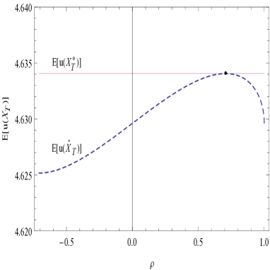
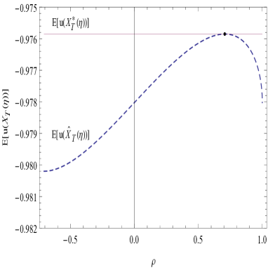
$\eta=1$ ($log$ utility)	$\eta=2$

Figure 1: Expected utility as a function of $\rho$ for a CRRA investor, with and without dependence constraint.

Assume that $t=T/2$ for the numerical application so that $S_{T/2}$ is the benchmark. Using an initial wealth $W_{0}=100$ and the same set of parameters as in the previous section, $\mu=0.06,$ $r=0.02,$ $\sigma=0.3$ and $T=1.$ Figure 1 plots the expected utility as a function of $\rho$ for the constrained payoff ($\widehat{X}_{T}$) and we have an horizontal line corresponding to the expected utility of $X_{T}^{\ast}$. Note that they share exactly one common point corresponding to the level of correlation found in (37).

5.2 Target probability maximization

Target probability maximizers are investors who, for a given budget (initial wealth) and a given time frame, want to maximize the probability that the final wealth achieves some fixed target $b$. In a Black–Scholes financial market model, Browne (1999) and Cvitanic̀ and Spivak (1999) derive the optimal investment strategy for these investors using stochastic control theory and show that it is optimal to purchase a digital option written on the risky asset. We show that their results follow from Theorem 2.2 in a more straightforward way.

Proposition 5.6 (Browne’s original problem).

Let $W_{0}$ be the initial wealth and let $b>W_{0}e^{rT}$ be the desired target. The solution to the following target probability maximization problem,

$$\underset{X_{T}\geqslant 0,\text{ }c_{0}(X_{T})=W_{0}}{\max}\mathbb{P}[X_{T}\geqslant b],$$ (39)

is given by the payoff

$$X_{T}^{\ast}=b\,\mathds{1}_{\{S_{T}>\lambda\}},$$ (40)

in which $\lambda$ is given by $b\mathbb{E}\left(\xi_{T}\mathds{1}_{\{S_{T}>\lambda\}}\right)=W_{0}$.

The proof of this proposition is provided in Appendix C.3. In a Black–Scholes market one easily verifies that $\lambda=S_{0}\exp\left({(r-\frac{\sigma^{2}}{2})T-\sigma\sqrt{T}\Phi^{-1}\left(\frac{W_{0}e^{rT}}{b}\right)}\right)$. $\Box$

A target probability maximizing strategy is essentially an all-or-nothing strategy. Intuitively, investors might not be attracted by the design of the optimal payoff, which maximizes the probability beating a fixed target. The obtained wealth depends solely on the ultimate value of the underlying risky asset, which makes it highly dependent on final market behavior and thus prone to unexpected and brutal changes. Our first extension concerns the case of a stochastic target, so that preferences become state-dependent.

Theorem 5.7 (Target probability maximization with a random target).

Let $W_{0}$ be the initial wealth and let $B$ be the random target such that $(B,S_{T})$ has a density. The solution to the random target probability maximization problem,

$$\underset{X_{T}\geqslant 0,\text{ }c_{0}(X_{T})=W_{0}}{\max}\mathbb{P}[X_{T}\geqslant B],$$ (41)

is given by the payoff

$$X_{T}^{\ast}=B\mathds{1}_{\left\{B{\xi_{T}}<\lambda\right\}},$$ (42)

in which $\lambda$ is implicitly given by $\mathbb{E}\left[B\xi_{T}\mathds{1}_{\left\{B\xi_{T}<\lambda\right\}}\right]=W_{0}$.

The proof of this proposition is provided in Appendix C.4. $\Box$

Our second extension assumes a fixed dependence with a benchmark in the financial market. We now consider the problem of an investor who, for a given budget, aims to maximize the probability that the final wealth will achieve some fixed target while preserving a certain dependence with a benchmark.

Theorem 5.8 (Target probability maximization with a random benchmark).

Let $W_{0}$ be the initial wealth and let $b>W_{0}e^{rT}$ the desired target for final wealth. Assume that the pair $(A_{T},S_{T})$ has a density. Then the solution to the target probability optimization problem with random benchmark $A_{T}$,

$$\underset{\begin{subarray}{c}X_{T}\geqslant 0,c_{0}(X_{T})=W_{0},\\ \mathcal{C}_{(X_{T},A_{T})}=C\end{subarray}}{\max}\mathbb{P}[X_{T}\geqslant b],$$ (43)

is given by

$$X_{T}^{\ast}=b\mathds{1}_{\left\{Z_{T}>\lambda\right\}},$$ (44)

in which $\lambda$ is determined by $b\mathbb{E}\left[\xi_{T}\mathds{1}_{\left\{Z_{T}>\lambda\right\}}\right]=W_{0}$ and $Z_{T}$ is defined as in (32).

The proof of this result is provided in Appendix C.5. $\Box$

The result derived in Theorem 5.8 holds in particular when $A_{T}=S_{t}$ ($0<t<T$) and when $C$ is a Gaussian copula with correlation coefficient $\rho.$ Then, the optimal solution is explicit and equal to

$$X_{T}^{\ast}=b\mathds{1}_{\left\{S_{t}^{\alpha}S_{T}>\lambda\right\}},$$ (45)

with $\alpha=\sqrt{\frac{T-t}{t(1-\rho^{2})}}\rho-1,$ and $\lambda=S_{0}^{\alpha+1}\exp\left({(r-\frac{\sigma^{2}}{2})(\alpha t+T)-\sigma\sqrt{k}\Phi^{-1}\left(\frac{W_{0}e^{rT}}{b}\right)}\right)$ with $k=(\alpha+1)^{2}t+(T-t)=\frac{T-t}{1-\rho^{2}}$. The proof of (45) is provided in Appendix C.6.

Illustration of target probability maximization

Let us compare the payoffs that arise from the unconstrained target probability maximization problem in Theorem 5.6 and the constrained maximization problem in Theorem 5.8. We use the same set of parameters as in Section 5.1, i.e., $\mu=0.06,$ $r=0.02,$ $\sigma=0.3$ and $T=1.$ We also take $S_{0}=100$ and $b=106$. In Figure 2, we plot for both payoffs their expected value as a function of $\rho$. The optimum for the unconstrained target optimization problem in Theorem 5.6 is given by $b\mathds{1}_{\{S_{T}>\lambda_{1}\}}$ in which $\lambda_{1}$ is such that the budget constraint is satisfied. Its expected value is given as

$$\mathbb{E}\left[b\mathds{1}_{\left\{S_{T}>\lambda_{1}\right\}}\right]=b{\Phi}\left[\theta\sqrt{T}+{\Phi}^{-1}\left[\frac{W_{0}e^{rT}}{b}\right]\right].$$

By similar reasoning, we find for the expected value of the optimum of Theorem 5.8,

$$\mathbb{E}\left[b\mathds{1}_{\left\{S_{t}^{\alpha}S_{T}>\lambda_{2}\right\}}\right]=b{\Phi}\left[\theta\frac{\alpha t+T}{\sqrt{k}}+{\Phi}^{-1}\left[\frac{W_{0}e^{rT}}{b}\right]\right],$$

in which $\alpha=\sqrt{\frac{T-t}{t(1-\rho^{2})}}\rho-1,$ $k=\frac{T-t}{1-\rho^{2}}$ and $\lambda_{2}$ is such that the budget constraint is satisfied. Note that the expected values are proportional to the probabilities to beat the target value $b$. We observe that in the constrained target probability maximization problem the expected value (and the corresponding success probability) is smaller than in the unconstrained problem.

Figure 2: Expected payoff as a function of $\rho$ for the different target probability maximization strategies considered in Theorem 5.6 and Theorem 5.8.

6 Final remarks

In this paper, we introduce a state-dependent version of the optimal investment problem. We deal with investors who target a known wealth distribution at maturity (as in the traditional setting) and additionally desire a particular interaction with a random benchmark. We show that optimal contracts depend at most on two underlying assets, or on one asset evaluated at two different dates, and we are able to characterize and determine them explicitly. Our characterization of optimal strategies allows us to extend the classical expected utility optimization problem of Merton to the state-dependent situation. Throughout the paper, we have assumed that the state-price density process $\xi_{T}$ is a decreasing functional of the risky asset price $S_{T}$ and that there is a single risky asset. It is possible to relax these assumptions and yet still to provide explicit representations of optimal payoffs. However, the optimality is then no longer related to path-independence properties.

Throughout the paper, we assumed that $\xi_{T}$ is decreasing in $S_{T}$ (in (2)). Moreover, we use the one-dimensional Black-Scholes model to illustrate our findings. However, the case of multidimensional markets described by a price process $(S_{t}^{(1)},\dots,S_{t}^{(d)})_{t}$ is essentially included in the results presented in this paper, assuming that the state-price density process $(\xi_{t})_{t}$ of the risk-neutral measure chosen for pricing is of the form $\xi_{t}=g_{t}\left(h_{t}(S_{t}^{(1)},\dots,S_{t}^{(d)})\right)$ with some real functions $g_{t}$, $h_{t}$ (as in Bernard, Maj and Vanduffel (2011) who considered the state-independent case). All results in the paper apply by replacing the one-dimensional stock price process $S_{t}$ by the one-dimensional process $h_{t}(S_{t}^{(1)},\dots,S_{t}^{(d)})$. In addition, we have assumed that asset prices are continuously distributed, which amounts essentially to assuming that the state-price density process $\xi_{t}$ is continuously distributed at any time. An extension to the case in which $\xi_{t}$ may have atoms is possible but not in the scope of the present paper.

A straightforward extension of the results presented in this paper is to consider the market model of Platen and Heath (2006) using the Growth Optimal Portfolio (GOP). Its origins can be traced back to Kelly (1956). It consists of replacing the state-price density process $\xi_{t}$ by $1/S_{t}^{\ast}$, where $S_{t}^{\ast}$ denotes the value of the GOP at time $t$. In the Black-Scholes setting, $S_{t}^{\ast}$ is simply the value of one unit investment in a constant-mix strategy, where a fraction $\frac{\theta}{\sigma}$ is invested in the risky asset and the remaining fraction $1-\frac{\theta}{\sigma}$ in the bank account. It is easy to prove that this strategy is optimal for an expected log-utility maximizer. Using a milder notion of arbitrage, Platen and Heath (2006) argue that, in general, the price of (non-negative) payoffs could be achieved using the pricing rule (1) where the role of $\xi_{T}$ is now played by the inverse of the GOP. Hence, our results are also valid in their setting, where the GOP is taken as the reference (see Bernard et al. (2014d) for an example).

Appendix A Proofs

Throughout the paper and the different proofs, we make repeatedly use of the following lemmas. The first lemma gives a restatement of the classical Hoeffding–Fréchet bounds going back to the early work of Hoeffding (1940) and Fréchet (1940), (1951).

Lemma A.1 (Hoeffding–Fréchet bounds).

Let $(X,Y)$ be a random pair and $U$ uniformly distributed on $(0,1)$. Then

$$\mathbb{E}\left[F_{X}^{-1}(U)F_{Y}^{-1}(1-U)\right]\leqslant\mathbb{E}\left[XY\right]\leqslant\mathbb{E}\left[F_{X}^{-1}(U)F_{Y}^{-1}(U)\right].$$ (46)

The upper bound for $\mathbb{E}\left[XY\right]$ is attained if and only if $(X,Y)$ is comonotonic, i.e. $(X,Y)\sim(F_{X}^{-1}(U),F_{Y}^{-1}(U)).$ Similarly, the lower bound for $\mathbb{E}\left[XY\right]$ is attained if and only if $(X,Y)$ is anti-monotonic, i.e. $(X,Y)\sim(F_{X}^{-1}(U),F_{Y}^{-1}(1-U)).$

The following lemma combines special cases of two classical construction results. The Rosenblatt transformation describes a transform of a random vector to iid uniformly distributed random variables (see Rosenblatt (1952)). The second result is a special form of the standard recursive construction method for a random vector with given distribution out of iid uniform random variables due to O’Brien (1975), Arjas and Lehtonen (1978) and Rüschendorf (1981).

Lemma A.2 (Construction method).

Let $(X,Y)$ be a random pair and assume that $F_{Y|X=x}(\cdot)$ is continuous $\forall x$. Denote $V=F_{Y|X}(Y).$ Then $V$ is uniformly distributed on $(0,1)$ and independent of $X.$ It is also increasing in $Y$ conditionally on $X$. Furthermore, for every variable $Z$, $(X,$ $F_{Z|X}^{-1}(V))\sim(X,Z).$

For the proof of the first part note that by the continuity assumption on $F_{Y\mid X=x}$ we get from the standard transformation

$$\left(V\mid X=x\right)\sim\left(F_{Y\mid X=x}(Y)\mid X=x\right)\sim U(0,1),\quad\forall x.$$

Clearly $V\sim U(0,1).$ Furthermore, the conditional distribution $F_{V\mid X=x}$ does not depend on $x$ and thus $V$ and $X$ are independent. For the second part one gets by the usual quantile construction that $F_{Z\mid X=x}^{-1}(V)$ has distribution function $F_{Z\mid X=x}$. This implies that $(X,F_{Z\mid X}^{-1}(V))$ $\sim$ $(X,Z)$ since both sides have the same first marginal distribution and the same conditional distribution.

Lemma A.3.

Let ($X,Y)$ be jointly normally distributed. Then, conditionally on $Y,$ $X$ is normally distributed and,

$$\mathbb{E}(X|Y) = \mathbb{E}(X)+\frac{\mathop{\mathrm{cov}}(X,Y)}{\mathop{\mathrm{var}}(Y)}(Y-\mathbb{E}(Y)$$

$$var(X|Y) = (1-\rho^{2})\mathop{\mathrm{var}}(X).$$

Denote the density of $Y$ by $f_{Y}(y)$. One has,

$$\int_{-\infty}^{c}e^{a+by}f_{Y}(y)dy=e^{a+b\mathbb{E}(Y)+\frac{b^{2}}{2}\mathop{\mathrm{var}}(Y)}\frac{1}{\sqrt{2\pi\mathop{\mathrm{var}}(Y)}}\int_{-\infty}^{c}e^{-\frac{1}{2}\left(\frac{y-(\mathbb{E}(Y)+b\mathop{\mathrm{var}}(Y))}{\sqrt{\mathop{\mathrm{var}}(Y)}}\right)^{2}}dy.$$

The results in this lemma are well-known and we omit its proof. $\Box$

A.1 Proof of Proposition 2.1

Let $U=F_{S_{T}}(S_{T})$ a uniformly distributed variable on $(0,1).$ Consider a payoff $X_{T}$. One has,

$$c_{0}(X_{T}) = \mathbb{E}\left[X_{T}\xi_{T}\right]\geqslant\mathbb{E}\left[F_{X_{T}}^{-1}(U)\xi_{T}\right]=c_{0}(X_{T}^{{*}}),$$

where the inequality follows from the fact that $F_{X_{T}}^{-1}(U)$ and $\xi_{T}$ are anti-monotonic and using the Hoeffding–Fréchet bounds in Lemma A.1. Hence, $X_{T}^{*}=F^{-1}(F_{S}(S_{T}))$ is the cheapest payoff with cdf $F.$ Similarly, the most expensive payoff with cdf $F$ writes as $Z_{T}^{{*}}=F^{-1}(1-F_{S}(S_{T}))$. Since $c$ is the price of a payoff $X_{T}$ with cdf $F$, one has

$$c\in[c_{0}(X_{T}^{{*}}),c_{0}(Z_{T}^{{*}})].$$

If $c=c_{0}(X_{T}^{{*}})$ then $X_{T}^{{*}}$ is a solution. Similarly, if $c=c_{0}(Z_{T}^{{*}})$ then $Z_{T}^{{*}}$ is a solution. Next, let $c\in(c_{0}(X_{T}^{{*}}),c_{0}(Z_{T}^{{*}}))$ and define the payoff $f_{a}(S_{T})$ with $a\in\mathbb{R}$,

$$f_{a}(S_{T})=F^{-1}\left[(1-F_{S_{T}}(S_{T}))\mathds{1}_{S_{T}\leqslant a}+(F_{S_{T}}(S_{T})-F_{S_{T}}(a))\mathds{1}_{S_{T}>a}\right].$$

Then $f_{a}(S_{T})$ is distributed with cdf $F$. The price $c_{0}(f_{a}(S_{T}))$ of this payoff is a continuous function of the parameter $a$. Since $\lim_{a\rightarrow 0^{+}}c_{0}(f_{a}(S_{T}))=c_{0}(X_{T}^{{*}})$ and $\lim_{a\rightarrow+\infty}c_{0}(f_{a}(S_{T}))=c_{0}(Z_{T}^{{*}})$, using the theorem of intermediary values for continuous functions, there exists $a^{\raisebox{-1.50694pt}{\footnotesize*}}$ such that $c_{0}(f_{a^{\raisebox{-3.22916pt}{\scriptsize*}}}(S_{T}))=c$. This ends the proof. $\Box$

A.2 Proof of Corollary 2.3

Let $X_{T}\sim F$ be cost-efficient. Then $X_{T}$ solves (6) and Theorem 2.2 implies that $X_{T}=F^{-1}(F_{S_{T}}(S_{T}))$ almost surely. Reciprocally, let $X_{T}\sim F$ be increasing in $S_{T}.$ Then, by our continuity assumption, $X_{T}=F^{-1}(F_{S_{T}}(S_{T}))$ almost surely and thus $X_{T}$ is cost-efficient. $\Box$

A.3 Proof of Theorem 3.2

The idea of the proof is very similar to the proof of Proposition 2.1. Let $U$ be given by $U=F_{S_{T}|A_{T}}(S_{T}).$ It is uniformly distributed over $(0,1)$ and independent of $A_{T}$ (see Lemma A.2). Furthermore, conditionally on $A_{T},$ $U$ is increasing in $S_{T}$. Consider next a payoff $X_{T}$ and note that $F_{X_{T}|A_{T}}^{-1}(U)\sim X_{T}.$ We find that

$$c_{0}(X_{T}) = \mathbb{E}\left[X_{T}\xi_{T}\right]=\mathbb{E}[\mathbb{E}[\left.X_{T}\xi_{T}\right|A_{T}]]$$ (47)

$$\geqslant \mathbb{E}\left[\mathbb{E}\left[\left.F_{X_{T}|A_{T}}^{-1}(U)\xi_{T}\right|A_{T}\right]\right]=\mathbb{E}\left[F_{X_{T}|A_{T}}^{-1}(U)\xi_{T}\right],$$

where the inequality follows from the fact that $F_{X_{T}|A_{T}}^{-1}(U)$ and $\xi_{T}$ are conditionally (on $A_{T}$) anti-monotonic and using (46) in Lemma A.1 for the conditional expectation (conditionally on $A_{T}$). Similarly, one finds that

$$c_{0}(X_{T})\leqslant\mathbb{E}\left[F_{X_{T}|A_{T}}^{-1}(1-U)\,\xi_{T}\right].$$

Next we define the uniform $(0,1)$ distributed variable,

$$g_{a}(S_{T})=(1-F_{S_{T}}(S_{T}))\mathds{1}_{S_{T}\leqslant a}+(F_{S_{T}}(S_{T})-F_{S_{T}}(a))\mathds{1}_{S_{T}>a}.$$

We observe that thanks to Lemma A.2, $F_{g_{a}(S_{T})|A_{T}}(g_{a}(S_{T}))$ is independent of $A_{T}$ and also that $f_{a}\left(S_{T},A_{T}\right)$ given as

$$f_{a}\left(S_{T},A_{T}\right)=F_{X_{T}|A_{T}}^{-1}(F_{g_{a}(S_{T})|A_{T}}(g_{a}(S_{T})))$$

is a twin with the desired joint distribution $G$ with $A_{T}.$ Denote by $X_{T}^{*}=F_{X_{T}|A_{T}}^{-1}(U)$ and by $Z_{T}^{{*}}=F_{X_{T}|A_{T}}^{-1}(1-U)$. Note that $X_{T}^{*}=f_{0}\left(S_{T},A_{T}\right)$ and $Z_{T}^{*}=f_{1}\left(S_{T},A_{T}\right)$ almost surely. The same discussion as in the proof of Proposition 2.1 applies here. When $c=c_{0}(X_{T}^{*})$ then $X_{T}^{*}$ is a twin with the desired properties. Similarly, when $c=c_{0}(Z_{T}^{*})$ then $Z_{T}^{*}$ is a twin with the desired properties. Otherwise, when $c\in(c_{0}(X_{T}^{*}),c_{0}(Z_{T}^{*}))$ then the continuity of $c_{0}(f_{a}\left(S_{T},A_{T}\right))$ with respect to $a$ ensures that there exists $a^{*}$ such that $c:=c_{0}(f_{a^{*}}\left(S_{T},A_{T}\right))$. Thus, $f_{a^{*}}\left(S_{T},A_{T}\right)$ is a twin with the desired joint distribution $G$ with $A_{T}$ and with cost $c$. This ends the proof. $\Box$

A.4 Proof of Theorem 3.3

Let $0<t<T.$ It follows from Lemma A.2 that $F_{S_{t}|S_{T}}(S_{t})$ is uniformly distributed on $(0,1)$ and independent of $S_{T}.$ Let the twin $f(S_{t},S_{T})$ be given as

$$f(S_{t},S_{T}):=F_{X_{T}|S_{T}}^{-1}(F_{S_{t}|S_{T}}(S_{t})).$$

Using Lemma A.2 again, one finds that $(f(S_{t},S_{T}),S_{T})\sim(X_{T},S_{T})\sim G.$ This also implies,

$$c_{0}(f(S_{t},S_{T})) = \mathbb{E}\left[f(S_{t},S_{T})\xi_{T}\right]=\mathbb{E[}X_{T}\xi_{T}]=c_{0}(X_{T}),$$

and this ends the proof. $\Box$

A.5 Proof of Theorem 3.4

It follows from Lemma A.2 that $U=F_{S_{T}|A_{T}}(S_{T})$ is uniformly distributed on $(0,1)$, stochastically independent of $A_{T}$ and increasing in $S_{T}$ conditionally on $A_{T}$. Let the twin $X_{T}^{*}$ be given as

$$X_{T}^{*}=F_{X_{T}|A_{T}}^{-1}(U).$$

Invoking Lemma A.2 again, $(X_{T}^{*},A_{T})\sim(X_{T},A_{T})\sim G.$ Moreover,

$$c_{0}(X_{T})=\mathbb{E}\left[X_{T}\xi_{T}\right] = \mathbb{E}[\mathbb{E}[\left.X_{T}\xi_{T}\right|A_{T}]]$$

$$\geqslant \mathbb{E}\left[\mathbb{E}\left[\left.F_{X_{T}|A_{T}}^{-1}(U)\xi_{T}\right|A_{T}\right]\right]$$

$$= \mathbb{E}\left[F_{X_{T}|A_{T}}^{-1}(U)\xi_{T}\right]=c_{0}(X_{T}^{*})$$

where the inequality follows from the fact that $F_{X_{T}|A_{T}}^{-1}(U)$ and $S_{T}$ are conditionally (on $A_{T}$) comonotonic and using (46) in Lemma A.1 for the conditional expectation (conditionally on $A_{T}$). $\Box$

A.6 Proof of Corollary 3.5

Let us first assume that $X_{T}$ is a cheapest twin. By Theorem 3.4, $X_{T}$ is (almost surely) equal to $X_{T}^{{*}}$ as defined by (14) which is, conditionally on $A_{T}$, increasing in $S_{T}$. Reciprocally, we now assume that $X_{T}=f\left(S_{T},A_{T}\right)$ is conditionally on $A_{T}$ increasing in $S_{T}$. Hence $X_{T}=F_{X_{T}|A_{T}}^{-1}\left(F_{S_{T}|A_{T}}\left(S_{T}\right)\right)$ almost surely, which means it is a solution to (13) and thus a cheapest twin. $\Box$

Appendix B Security design

B.1 Twin of the fixed strike (continuously monitored) geometric Asian call option

Expression (11) allows us to find twins satisfying the constraint (19) on the dependence with the benchmark $S_{T}$. Using Lemma A.3 we find that

$$\ln(S_{t}/S_{0})|\ln(S_{T}/S_{0})\sim\mathcal{N}\left(\frac{t}{T}\ln\left(\frac{S_{T}}{S_{0}}\right),\sigma^{2}t\left(1-\frac{t}{T}\right)\right),$$

and thus

$${F_{S_{t}|S_{T}}(S_{t})}=\Phi\left(\frac{\ln\left(\frac{S_{t}S_{0}^{\frac{t}{T}-1}}{S_{T}^{\frac{t}{T}}}\right)}{\sigma\sqrt{\frac{tT-t^{2}}{T}}}\right).$$

Furthermore, the couple ($\ln\left(G_{T}\right),\ln\left(S_{T}\right))$ is bivariate normally distributed with mean and variance for the marginal distributions that are given as $\mathbb{E}[\ln(G_{T})]=\ln S_{0}+\left(\mu-\frac{1}{2}\sigma^{2}\right)\frac{T}{2}$, $\hbox{var}[\ln(G_{T})]=\frac{\sigma^{2}T}{3}$ and $\mathbb{E}[\ln(S_{T})]=\ln S_{0}+\left(\mu-\frac{1}{2}\sigma^{2}\right){T}$, $\hbox{var}[\ln(S_{T})]=\ {\sigma^{2}T}$. For the correlation coefficient one has $\rho(\ln(S_{T}),\ln(G_{T}))=\frac{\sqrt{3}}{2}.$ Applying Lemma A.3 again one finds that,

$$\ln(G_{T})|\ln(S_{T})\sim\mathcal{N}\left(\ln\left(S_{0}^{1/2}S_{T}^{1/2}\right),\frac{\sigma^{2}T}{12}\right),$$ (48)

and thus,

$$F_{G_{T}|S_{T}}(x)=\Phi\left(\frac{\ln(x)-\ln\left(S_{0}^{1/2}S_{T}^{1/2}\right)}{\frac{\sigma\sqrt{T}}{2\sqrt{3}}}\right).$$

Therefore,

$$F_{G_{T}|S_{T}}^{-1}(y)=\exp\left(\ln\left(S_{0}^{1/2}S_{T}^{1/2}\right)+\frac{\sigma\sqrt{T}}{2\sqrt{3}}\Phi^{-1}(y)\right).$$

The expression of $R_{T}(t)$ given in (21) is then straightforward to derive.

For choosing a specific twin among others, we suggest to maximize $\rho\left(\ln R_{T}(t),\ln G_{T}\right)$. First, we calculate,

$$\mathop{\mathrm{cov}}\left(\ln S_{T},\frac{1}{T}\int_{0}^{T}\ln\left(S_{s}\right)ds\right) = \frac{1}{T}\int_{0}^{T}\mathop{\mathrm{cov}}\left(\ln S_{T},\ln\left(S_{s}\right)\right)ds$$

$$= \frac{\sigma^{2}}{T}\int_{0}^{T}\left(s\wedge T\right)ds=\frac{\sigma^{2}T}{2}.$$

Furthermore, by denoting $a=\frac{1}{2}-\frac{1}{2\sqrt{3}}\sqrt{\frac{T-t}{t}}$, $b=\frac{T}{t}\frac{1}{2\sqrt{3}}\sqrt{\frac{t}{T-t}}$ and $c=\frac{1}{2}-\frac{1}{2\sqrt{3}}\sqrt{\frac{t}{T-t}}$, equation (21) may be rewritten as $\ln R_{T}\left(t\right)=a\ln S_{0}+b\ln S_{t}+c\ln S_{T}$. The covariance being bilinear, one then has,

$${\mathop{\mathrm{cov}}\left(\ln R_{T}\left(t\right),\ln G_{T}\right)} = b\mathop{\mathrm{cov}}\left(\ln S_{t},\frac{1}{T}\int_{0}^{T}\ln\left(S_{s}\right)ds\right)+c\mathop{\mathrm{cov}}\left(\ln S_{T},\frac{1}{T}\int_{0}^{T}\ln\left(S_{s}\right)ds\right)$$

$$= \frac{\sigma^{2}}{2}\left(\frac{T}{2}+\frac{\sqrt{t}\sqrt{T-t}}{2\sqrt{3}}\right).$$

Denote by $\sigma_{\ln R_{T}\left(t\right)}$ and by $\sigma_{\ln G_{T}}$ the respective standard deviations. For the correlation we find that

$$\rho\left(\ln R_{T}\left(t\right),\ln G_{T}\right)=\frac{\mathop{\mathrm{cov}}\left(\ln R_{T}\left(t\right),\ln G_{T}\right)}{\sigma_{\ln R_{T}\left(t\right)}\sigma_{\ln G_{T}}} = \frac{3}{4}+\frac{\sqrt{3}\sqrt{\left(T-t\right)t}}{4T}.$$

Hence $\rho\left(\ln R_{T}\left(t\right),\ln G_{T}\right)$ is maximized for $t=\frac{T}{2}$. $\Box$

B.2 Twin of the floating strike (continuously monitored) geometric Asian put option

We first recall from equation (48) that,

$$\ln(G_{T})|\ln(S_{T})\sim\mathcal{N}\left(\ln\left(S_{0}^{\frac{1}{2}}S_{T}^{\frac{1}{2}}\right),\frac{\sigma^{2}T}{12}\right).$$

Therefore $Y_{T}=(G_{T}-S_{T})^{+}$ has the following conditional cdf

$$\mathbb{P}(Y_{T}\leqslant y|S_{T}=s)=\Phi\left(\frac{\ln(s+y)-\ln\left(S_{0}^{1/2}s^{1/2}\right)}{\frac{\sigma\sqrt{T}}{2\sqrt{3}}}\right)\mathds{1}_{y\geqslant 0}$$

Then

$$F_{Y_{T}|S_{T}}^{-1}(z)=\left(S_{0}^{\frac{1}{2}}S_{T}^{\frac{1}{2}}e^{\frac{\sigma}{2}\sqrt{\frac{T}{3}}\Phi^{-1}(z)}-S_{T}\right)^{+}.$$

Therefore $F_{Y_{T}|S_{T}}^{-1}\left(F_{S_{t}|S_{T}}(S_{t}))\right)$ can then easily be computed and after some calculations it simplifies to (24). $\Box$

B.3 Cheapest Twin of the floating strike (continuously monitored) geometric Asian put option

Applying Lemma A.3 we find,

$$\ln(S_{T})|\ln(G_{T})\sim\mathcal{N}\left(\ln\left(\frac{G_{T}^{3/2}}{S_{0}^{\frac{1}{2}}}\right)+\frac{1}{4}\left(\mu-\frac{\sigma^{2}}{2}\right)T,\ \frac{\sigma^{2}T}{4}\right).$$

Hence,

$${F_{S_{T}|G_{T}}(S_{T})})=\Phi\left(\frac{\ln\left(\frac{S_{T}S_{0}^{\frac{1}{2}}}{G_{T}^{\frac{3}{2}}}\right)-\left(\mu-\frac{\sigma^{2}}{2}\right)\frac{T}{4}}{\frac{\sigma\sqrt{T}}{2}}\right).$$ (49)

Furthermore, $Y_{T}=(G_{T}-S_{T})^{+}$ has the following conditional cdf,

$$P(Y_{T}\leqslant y|G_{T}=g)=\left\{\begin{array}[]{cl}1&\hbox{if}\ y\geqslant g,\\ \Phi\left(\frac{\ln\left(\frac{g^{3/2}}{S_{0}^{\frac{1}{2}}}\right)+\frac{1}{4}\left(\mu-\frac{\sigma^{2}}{2}\right)T-\ln(g-y)}{\frac{\sigma\sqrt{T}}{2}}\right)&\hbox{if}\ 0\leqslant y\leqslant g,\\ 0&\hbox{if}\ y<0.\end{array}\right.$$

Then

$$F_{Y_{T}|G_{T}}^{-1}(z)=\left(G_{T}-\frac{G_{T}^{\frac{3}{2}}}{S_{0}^{\frac{1}{2}}}e^{\frac{1}{4}\left(\mu-\frac{\sigma^{2}}{2}\right)T-\frac{\sigma}{2}\sqrt{T}\Phi^{-1}(z)}\right)^{+}.$$

Replacing $z$ by the expression (49) for ${F_{S_{T}|G_{T}}(S_{T})})$ derived above, then gives rise to expression (25). $\Box$

B.4 Derivation of prices (26) and (27)

Price (26)

Let us observe that,

$$\begin{array}[]{rcl}\left(G_{T}-S_{T}\right)^{+}&=&G_{T}\left(1-\frac{S_{T}}{G_{T}}\right)^{+}=S_{0}e^{Y}\left(1-e^{Z}\right)^{+},\end{array}$$

where $Z=X-Y,$ $Y=\ln\left(\frac{G_{T}}{S_{0}}\right),$ $X=\ln\left(\frac{S_{T}}{S_{0}}\right)$. We find, with respect to the risk neutral measure $\mathbb{Q},$

$$\mathbb{E}_{\mathbb{Q}}\left[\left(G_{T}-S_{T}\right)^{+}\right] = S_{0}\mathbb{E}_{\mathbb{Q}}\left(\mathbb{E}_{\mathbb{Q}}\left[e^{Y}|Z\right]\left(1-e^{Z}\right)^{+}\right)$$

$$= S_{0}\mathbb{E}_{\mathbb{Q}}\left[\left(e^{\mathbb{E}_{\mathbb{Q}}(Y|Z)+\frac{1}{2}\mathop{\mathrm{var}_{\mathbb{Q}}}(Y|Z)}-e^{\mathbb{E}_{\mathbb{Q}}(Y|Z)+\frac{1}{2}\mathop{\mathrm{var}_{\mathbb{Q}}}(Y|Z)+Z}\right)^{+}\right].$$

We now compute (still with respect to $\mathbb{Q})$,

$$\mathbb{E}_{\mathbb{Q}}(Y|Z) = \mathbb{E}_{\mathbb{Q}}(Y)+\frac{\mathop{\mathrm{cov}_{\mathbb{Q}}}(Y,Z)}{\mathop{\mathrm{var}_{\mathbb{Q}}}(Z)}(Z-\mathbb{E}_{\mathbb{Q}}(Z))=\left(r-\frac{\sigma^{2}}{2}\right)\frac{T}{4}+\frac{1}{2}Z$$

$$\mathop{\mathrm{var}_{\mathbb{Q}}}(Y|Z) = (1-\rho^{2})\mathop{\mathrm{var}_{\mathbb{Q}}}(Y)=\frac{3}{4}\frac{\sigma^{2}T}{3}=\frac{\sigma^{2}T}{4}.$$

Hence,

$$\mathbb{E}_{\mathbb{Q}}\left(G_{T}-S_{T}\right)^{+} = S_{0}\mathbb{E}_{\mathbb{Q}}\left(e^{r\frac{T}{4}+\frac{1}{2}Z}-e^{r\frac{T}{4}+\frac{3}{2}Z}\right)^{+}$$

$$= S_{0}\int_{-\infty}^{0}e^{{}^{r\frac{T}{4}+\frac{1}{2}Z}}f_{Z}(z)dz-S_{0}\int_{-\infty}^{0}e^{r\frac{T}{4}+\frac{3}{2}Z}f_{Z}(z)dz,$$

where $f_{Z}(z)$ is now denoting the density of $Z$ under $\mathbb{Q}.$ Here $Z$ is normally distributed with parameters $(r-\frac{\sigma^{2}}{2})\frac{T}{2}$ and variance $\frac{\sigma^{2}T}{3}.$ Hence, taking into account Lemma A.3,

$${\mathbb{E}_{\mathbb{Q}}\left(G_{T}-S_{T}\right)^{+}} = S_{0}e^{r\frac{T}{2}-\sigma^{2}\frac{T}{12}}\Phi\left(\frac{-\left(r-\frac{\sigma^{2}}{2}\right)\frac{T}{2}-\frac{\sigma^{2}T}{6}}{\sqrt{\frac{\sigma^{2}T}{3}}}\right)-S_{0}e^{rT}\Phi\left(\frac{-\left(r-\frac{\sigma^{2}}{2}\right)\frac{T}{2}-\frac{\sigma^{2}T}{2}}{\sqrt{\frac{\sigma^{2}T}{3}}}\right)$$

Choose $f=\frac{-r\frac{T}{2}+\frac{\sigma^{2}T}{12}}{\sigma\sqrt{\frac{T}{3}}}$ to obtain (26).

Price (27)

One has,

$$\left(G_{T}-a\frac{G_{T}^{3}}{S_{T}}\right)^{+}=G_{T}\left(1-a\frac{G_{T}^{2}}{S_{T}}\right)^{+}=S_{0}e^{Y}\left(1-ce^{Z}\right)^{+}$$

where $Z=2Y-X,$ $Y=\ln\left(\frac{G_{T}}{S_{0}}\right),$ $X=\ln\left(\frac{S_{T}}{S_{0}}\right),$ $c=e^{\left(\mu-\frac{\sigma^{2}}{2}\right)\frac{T}{2}}.$ Hence, with respect to the risk neutral measure $\mathbb{Q},$

$$\mathbb{E}_{\mathbb{Q}}\left(G_{T}-a\frac{G_{T}^{3}}{S_{T}}\right)^{+} = S_{0}\mathbb{E}_{\mathbb{Q}}\left(\mathbb{E}_{\mathbb{Q}}(e^{Y}|Z)\left(1-ce^{Z}\right)^{+}\right)$$

$$= S_{0}\mathbb{E}_{\mathbb{Q}}\left(e^{\mathbb{E}_{\mathbb{Q}}(Y|Z)+\frac{1}{2}\mathop{\mathrm{var}_{\mathbb{Q}}}(Y|Z)}-ce^{\mathbb{E}_{\mathbb{Q}}(Y|Z)+\frac{1}{2}\mathop{\mathrm{var}_{\mathbb{Q}}}(Y|Z)+Z}\right)^{+}.$$

We now compute,

$$\mathbb{E}_{\mathbb{Q}}(Y|Z)=\left(r-\frac{\sigma^{2}}{2}\right)\frac{T}{2}+\frac{1}{2}Z\quad\mathrm{and}\quad\mathop{\mathrm{var}_{\mathbb{Q}}}(Y|Z)=\frac{\sigma^{2}T}{4}.$$

Hence,

$$\mathbb{E}_{\mathbb{Q}}\left(G_{T}-a\frac{G_{T}^{3}}{S_{T}}\right)^{+} = S_{0}\mathbb{E}_{\mathbb{Q}}\left(e^{r\frac{T}{2}-\frac{\sigma^{2}T}{8}+\frac{1}{2}Z}-ce^{r\frac{T}{2}-\frac{\sigma^{2}T}{8}+\frac{3}{2}Z}\right)^{+}$$

$$= S_{0}\int_{-\infty}^{\ln(c)}e^{{}^{r\frac{T}{2}-\frac{\sigma^{2}T}{8}+\frac{1}{2}Z}}f_{Z}(z)dz-S_{0}c\int_{-\infty}^{\ln(c)}e^{r\frac{T}{2}-\frac{\sigma^{2}T}{8}+\frac{3}{2}Z}f_{Z}(z)dz,$$

where $f_{Z}(z)$ is the density of $Z,$ under $\mathbb{Q}.$ Note that $Z$ is normally distributed with parameters $0$ and variance $\frac{\sigma^{2}T}{3}.$ Taking into account Lemma A.3,

$$\mathbb{E}_{\mathbb{Q}}\left(G_{T}-a\frac{G_{T}^{3}}{S_{T}}\right)^{+} = S_{0}e^{\frac{rT}{2}}\left(\Phi\left(d\right)e^{-\frac{\sigma^{2}T}{12}}-e^{\frac{\mu T}{2}}\Phi\left(d-\frac{\sigma\sqrt{T}}{\sqrt{3}}\right)\right)$$

where $d=\frac{-\ln(c)-\frac{\sigma^{2}T}{6}}{\sigma\sqrt{\frac{T}{3}}}=\frac{\frac{\sigma^{2}T}{12}-\mu\frac{T}{2}}{\sigma\sqrt{\frac{T}{3}}}$. $\Box$

Appendix C Portfolio Management

C.1 Proof of Theorem 5.2

Let $H_{T}=\mathbb{E}(\xi_{T}|Z_{T})=\varphi(Z_{T})$ and let $\widehat{\varphi}$ denote the projection of $\varphi$ on the cone $M_{\downarrow}$ defined as in (33) with respect to $L^{2}(\lambda_{[0,1]})$. Then we define $\widehat{X}_{T}$ and $k(\cdot)$ by

$$u^{\prime}(\widehat{X}_{T}):=\lambda\widehat{\varphi}(Z_{T}),$$

i.e. $\widehat{X}_{T}=\left(u^{\prime}\right)^{-1}(\lambda\widehat{\varphi}(Z_{T}))=:k(Z_{T})$ with $\lambda$ such that $\mathbb{E}[\xi_{T}\widehat{X}_{T}]=\mathbb{E}\left[\varphi(Z_{T})k(Z_{T})\right]=\int_{0}^{1}\varphi(t)k(t)dt=\varphi\cdot k=W_{0}$. By definition, $\widehat{X}_{T}$ is increasing in $Z_{T}$ since $\left(u^{\prime}\right)^{-1}$ is decreasing and $\widehat{\varphi}$ is decreasing (it belongs to $M_{\downarrow}$). As a consequence $\widehat{X}_{T}$ is increasing in $S_{T}$, conditionally on $A_{T}$. For any $Y_{T}=h(Z_{T})$ with a increasing function $h$, we have by concavity of $u$

$$u(Y_{T})-u(\widehat{X}_{t}) \leqslant u^{\prime}(\widehat{X}_{T})(Y_{T}-\widehat{X}_{T})=\lambda\widehat{\varphi}(Z_{T})(h(Z_{T})-k(Z_{T})).$$

Thus, we obtain

$$\mathbb{E}[u(Y_{T})]-\mathbb{E}[u(\widehat{X}_{T})]\leqslant\lambda\int_{0}^{1}\widehat{\varphi}(t)(h(t)-k(t))dt=\lambda\widehat{\varphi}\cdot(h-\Psi(\widehat{\varphi})),$$ (50)

where $\Psi(\widehat{\varphi})=\left(u^{\prime}\right)^{-1}(\lambda\widehat{\varphi})=k$ is increasing and $\Psi(t)=\left(u^{\prime}\right)^{-1}(\lambda t)$ is decreasing.

Now we use some properties of isotonic approximations (see Barlow et al. (1972)) and obtain

$$\widehat{\varphi}\cdot(h-\Psi(\widehat{\varphi})) = \widehat{\varphi}\cdot((-\Psi)(\widehat{\varphi})-(-h))$$

$$= \varphi\cdot(-\Psi)(\widehat{\varphi})-\widehat{\varphi}\cdot(-h)\qquad\text{{\small(see Theorem 1.7 in Barlow {et al.} \cite[citeyear]{\@@bibref{Year}{BBBB}{}{}})}}$$

$$= \varphi\cdot(-h)-\widehat{\varphi}\cdot(-h)\quad\phantom{x}\text{{\small both claims have price $W_{0}$}}$$

$$= (\varphi-\widehat{\varphi})\cdot(-h)\leqslant 0$$

by the projection equation (see Theorem 7.8 in Barlow et al. (1972)) using that $-h\in M_{\downarrow}$. As a result we obtain from (50) that

$$\mathbb{E}[u(Y_{T})]\leqslant\mathbb{E}[u(\widehat{X}_{T})],$$

i.e. $\widehat{X}_{T}$ is an optimal claim. $\Box$

C.2 Proofs of equations (36) and (38) in the example of subsection 5.1

We apply Theorem 5.1 to an investor with a power-utility. Then,

$$X_{T}^{\star}\left(\eta\right)=(u^{\prime})^{-1}(\lambda\xi_{T})=(\lambda\xi_{T})^{-\frac{1}{\eta}}$$ (51)

where $\lambda$ is chosen to meet the budget constraint, i.e.

$$\mathbb{E}[\xi_{T}(u^{\prime})^{-1}(\lambda\xi_{T})]=\mathbb{E}\left[\xi_{T}(\lambda\xi_{T})^{-\frac{1}{\eta}}\right]=\lambda^{-\frac{1}{\eta}}\mathbb{E}\left[\xi_{T}^{1-\frac{1}{\eta}}\right]=W_{0}$$ (52)

Since $\xi_{T}=\exp\left\{-rT-\frac{1}{2}\theta^{2}T-\theta Z_{T}\right\}$, we find that $\lambda^{-\frac{1}{\eta}}=W_{0}\exp\left\{-r\left(\frac{1-\eta}{\eta}\right)T-\frac{1}{2}\theta^{2}T\left(\frac{1-\eta}{\eta}\right)\frac{1}{\eta}\right\}$ and

$$X_{T}^{\star}\left(\eta\right)=(\lambda\xi_{T})^{-\frac{1}{\eta}}=W_{0}e^{-r\left(\frac{1-\eta}{\eta}\right)T-\frac{1}{2}\theta^{2}T\left(\frac{1-\eta}{\eta}\right)\frac{1}{\eta}-\frac{1}{\eta}\left[\frac{\theta}{\sigma}\left(\mu-\frac{\sigma^{2}}{2}\right)T-\left(r+\frac{\theta^{2}}{2}\right)T\right]}\left(\frac{S_{T}}{S_{0}}\right)^{\frac{\theta}{\sigma\eta}},$$

which can be simplified to find (36).

Next, we apply Theorem 5.2 with $A_{T}=S_{t}$, for some $t$ such that $t<T$. From Lemma A.3 we know

$$\ln(S_{T})|\ln(S_{t})\sim\mathcal{N}\left(\ln\left(St\right)+\left(\mu-\frac{\sigma^{2}}{2}\right)(T-t),\sigma^{2}(T-t)\right)$$

so that

$${F_{S_{T}|S_{t}}(S_{T})}=\Phi\left(\frac{\ln\left(\frac{S_{T}}{S_{t}}\right)-\left(\mu-\frac{\sigma^{2}}{2}\right)(T-t)}{\sigma\sqrt{T-t}}\right).$$

Because $C$ is a Gaussian copula, one has

$$C_{1|S_{t}}(x)=\Phi\left[\frac{\Phi^{-1}\left[x\right]-\rho\left(\frac{\ln\left(\frac{S_{t}}{S_{0}}\right)-\left(\mu-\frac{\sigma^{2}}{2}\right)t}{\sigma\sqrt{t}}\right)}{\sqrt{1-\rho^{2}}}\right]$$

and

$$C_{1|S_{t}}^{-1}(y)=\Phi\left[\sqrt{1-\rho^{2}}\Phi^{-1}\left[y\right]+\rho\left(\frac{\ln\left(\frac{S_{t}}{S_{0}}\right)-\left(\mu-\frac{\sigma^{2}}{2}\right)t}{\sigma\sqrt{t}}\right)\right].$$

This implies

$$\zeta_{T}=C_{1|S_{t}}^{-1}({F_{S_{T}|S_{t}}(S_{T})})=\Phi\left[\varpi_{T}\right],$$

where $\varpi_{T}$ is a function of $S_{T}$ and $S_{t}$ given by

$$\varpi_{T}=\sqrt{1-\rho^{2}}\left(\frac{\ln\left(\frac{S_{T}}{S_{t}}\right)-\left(\mu-\frac{\sigma^{2}}{2}\right)(T-t)}{\sigma\sqrt{T-t}}\right)+\rho\left(\frac{\ln\left(\frac{S_{t}}{S_{0}}\right)-\left(\mu-\frac{\sigma^{2}}{2}\right)t}{\sigma\sqrt{t}}\right).$$ (53)

Since $\xi_{T}=\alpha_{T}\left(\frac{S_{T}}{S_{0}}\right)^{-\beta}$ where $\alpha_{T}=\exp\left(\frac{\theta}{\sigma}\left(\mu-\frac{\sigma^{2}}{2}\right)T-\left(r+\frac{\theta^{2}}{2}\right)T\right)$, $\beta=\frac{\theta}{\sigma}$ and $\theta=\frac{\mu-r}{\sigma}$ (from (4)), one has

$$H_{T}=\mathbb{E}(\xi_{T}|\zeta_{T})=\mathbb{E}(\xi_{T}|\varpi_{T})=\delta e^{-\beta\mathop{\mathrm{cov}}\left(\ln\left(S_{T}\right),\varpi_{T}\right)\varpi_{T}},$$

for some $\delta>0$ and we find

$$H_{T}=\delta e^{-\theta\left(\rho\sqrt{t}+\sqrt{(1-\rho^{2})(T-t)}\right)\varpi_{T}}.$$

Note that conditions on the correlation coefficient imply that $H_{T}$ is decreasing in $\varpi_{T}$ and thus $H_{T}$ is decreasing in $Z_{T}.$ The optimal contract thus writes as

$$\widehat{X}_{T}:=\left(u^{\prime}\right)^{-1}\left(\lambda e^{-\theta\left(\rho\sqrt{t}+\sqrt{(1-\rho^{2})(T-t)}\right)\varpi_{T}}\right),$$ (54)

where $\lambda$ is chosen to meet the budget constraint.

When the investor has a power-utility, i.e., $u\left(x\right)=\frac{x^{1-\eta}}{1-\eta}$ so that $(u^{\prime})^{-1}\left(x\right)=x^{-\frac{1}{\eta}}$ we find that equation (54) reads as

$$\widehat{X}_{T}\left(\eta\right):=\lambda^{-\frac{1}{\eta}}e^{\frac{1}{\eta}\theta\left(\rho\sqrt{t}+\sqrt{(1-\rho^{2})(T-t)}\right)\varpi_{T}}$$ (55)

and the budget constraint (i.e., $\mathbb{E}\left[\xi_{T}\widehat{X}_{T}\left(\eta\right)\right]=W_{0}$) requires that

$$\mathbb{E}\left[e^{-rT}e^{-\frac{\theta^{2}}{2}T-\theta Z_{T}}\lambda^{-\frac{1}{\eta}}\exp\left[\frac{1}{\eta}\theta\left(\rho\sqrt{t}+\sqrt{(1-\rho^{2})(T-t)}\right)\varpi_{T}\right]\right]=W_{0},$$

where we have used the expressions for $\xi_{T}$ and $\widehat{X}_{T}\left(\eta\right)$. We find that

$$\lambda^{-\frac{1}{\eta}}=W_{0}e^{rT}e^{\theta^{2}\left(\rho\sqrt{t}+\sqrt{(1-\rho^{2})(T-t)}\right)^{2}\left(\frac{1}{\eta}-\frac{1}{2\eta^{2}}\right)}.$$

The optimal solution is then derived by using this expression into (55). $\Box$

C.3 Proof of Proposition 5.6

Assume that there exists an optimal solution to the target probability maximization problem. It is a maximization of a law-invariant objective and therefore it is path-independent. Denote it by $X_{T}^{*}:=f^{*}(S_{T}).$ Define $A_{0}=\{x\ |\ f^{*}(x)=0\}$, $A_{1}=\{x\ |\ f^{*}(x)=b\}$, $A_{2}=\{x\ |\ f^{*}(x)\in]0,b[\}$ and $A_{3}=\{x\ |\ f^{*}(x)>b\}$. We show that $\mathbb{P}(S_{T}\in A_{0}\cup A_{1})=1$ must hold. Assume $\mathbb{P}(S_{T}\in A_{0}\cup A_{1})<1$ so that $\mathbb{P}(S_{T}\in A_{2}\cup A_{3})>0.$ Define

$$Y=\left\{\begin{array}[]{cl}f^{*}(S_{T})&\hbox{for}\ S_{T}\in A_{0}\cup A_{1},\\ 0&\hbox{for}\ S_{T}\in A_{2},\\ b&\hbox{for}\ S_{T}\in A_{3}.\end{array}\right.$$

Then we observe that $Y=f^{*}(S_{T})$ on $A_{0}\cup A_{1}$ and $Y<f^{*}(S_{T})$ on $A_{2}\cup A_{3}.$ Since $\mathbb{P}(S_{T}\in A_{2}\cup A_{3})>0$ also $\mathbb{Q}(S_{T}\in A_{2}\cup A_{3})>0$ because $\mathbb{P}$ and the risk neutral probability $\mathbb{Q}$ are equivalent. Hence $c_{0}(Y)<W_{0}.$ Next we define $Z=b\mathds{1}_{S_{T}\in C}+Y\$ where we have chosen $C\subseteq A_{2}\cup A_{0}$ such that $c_{0}(b\mathds{1}_{S_{T}\in C})=W_{0}-c_{0}(Y).$ Since $\mathbb{P}(S_{T}\in C)>0$ one has that $\mathbb{P}(Z\geqslant b)>\mathbb{P}(Y\geqslant b)=\mathbb{P}(f^{*}(S_{T})\geqslant b).$ Hence $Z$ contradicts the optimality of $f^{*}(S_{T})$. Therefore $\mathbb{P}(S_{T}\in A_{0}\cup A_{1})=1.$ Hence $f^{*}(S_{T})$ can take only the values 0 or $b$. Since it is increasing in $S_{T}$ almost surely (by cost-efficiency) it must write as

$$f^{*}(S_{T})=b\mathds{1}_{S_{T}>a},$$

where $a$ is chosen such that the budget constraint is satisfied. $\Box$

C.4 Proof of Theorem 5.7

The (random) target probability maximization problem is given as

$$\max_{X_{T}\geqslant 0,c_{0}(X_{T})=W_{0}}\mathbb{P}[X_{T}\geqslant B].$$

Assume that there exists an optimal solution $X_{T}^{\ast}$ to this optimization problem. There are three steps in the proof.

1. The optimal payoff is of the form $f(S_{T},B)$.

2. The optimal payoff is of the form $B\mathds{1}_{h(S_{T},B)\in A}$.

3. The optimal payoff is of the form $B\mathds{1}_{B\xi_{T}<\lambda^{{\ast}}}$ for $\lambda^{{\ast}}>0$.

Step 1: We observe that $X_{T}^{\ast}$ has some joint distribution $G$ with $B.$ Theorem 3.2 implies there exists a twin $f(B,S_{T})$ such that $(f(B,S_{T}),B_{T})\sim(X_{T}^{\ast},B)\sim G$ and $c_{0}(f(B,S_{T}))=c_{0}(X_{T}^{\ast})=W_{0}$. Therefore $\mathbb{P}(f(B,S_{T})\geqslant B)=\mathbb{P}(X_{T}^{\ast}\geqslant B)$ and $\mathbb{P}(f(B,S_{T})\geqslant 0)=\mathbb{P}(X_{T}^{\ast}\geqslant 0)=1$. Thus $f(B,S_{T})$ is also an optimal solution.

Step 2: This is similar to the proof of Proposition 5.6, applied conditionally on $B.$ Define the sets $A_{0}=\{s,f(B,s)=0\}$, $A_{1}=\{s,f(B,s)=B\},$ then $\mathbb{P}(S_{T}\in A_{0}\cup A_{1}|B)=1$ and therefore $\mathbb{P}(S_{T}\in A_{0}\cup A_{1})=1$. Thus there exists a set $A$ and a function $h$ such that

$$f(B,S_{T})=B\mathds{1}_{h(S_{T},B)\in A}.$$

Step 3: Define $\lambda>0$ such that

$$\mathbb{P}(h(S_{T},B)\in A)=\mathbb{P}(B\xi_{T}<\lambda).$$

Observe that $\mathds{1}_{h(S_{T},B)\in A}$ and $\mathds{1}_{B\xi_{T}<\lambda}$ have the same distribution and that in addition, $B\xi_{T}$ is anti-monotonic with $\mathds{1}_{B\xi_{T}<\lambda}$. Therefore by applying Lemma A.1 one has that

$$c_{0}(B\mathds{1}_{B\xi_{T}<\lambda})=\mathbb{E}[B\xi_{T}\mathds{1}_{B\xi_{T}<\lambda}]\leqslant\mathbb{E}[B\xi_{T}\mathds{1}_{h(S_{T},B)\in A}]$$

and therefore the optimum must be of the form $B\mathds{1}_{B\xi_{T}<\lambda^{\ast}}$ where $\lambda^{\ast}>\lambda$ is determined such that $c_{0}(B\mathds{1}_{B\xi_{T}<\lambda^{\ast}})=W_{0}.$ $\Box$

C.5 Proof of Theorem 5.8

The target probability maximization problem is given by

$$\underset{\begin{subarray}{c}X_{T}\geqslant 0,\ c_{0}(X_{T})=W_{0},\\ \mathcal{C}_{(X_{T},A_{T})}=C\end{subarray}}{\max}\mathbb{P}[X_{T}\geqslant b]$$

Assume that there exists an optimal solution $X_{T}^{*}$ to this optimization problem. There are three steps in the proof.

1. The optimal payoff is of the form $f(S_{T},A_{T})$.

2. The optimal payoff is of the form $b\mathds{1}_{h(S_{T},A_{T})\in A}$.

3. The optimal payoff is of the form $A_{T}\mathds{1}_{Z_{T}>\lambda^{{*}}}$ for $\lambda^{{*}}>0$.

Step 1: We observe that $X_{T}^{*}$ has some joint distribution $G$ with $A_{T}.$ Theorem 3.2 implies there exists a twin $f(S_{T},A_{T})$ such that $(f(S_{T},A_{T}),A_{T})\sim(X_{T}^{*},A_{T})\sim G$ and $c_{0}(f(S_{T},A_{T}))=c_{0}(X_{T}^{*})=W_{0}$. Therefore $\mathbb{P}(f(S_{T},A_{T})\geqslant b)=\mathbb{P}(X_{T}^{*}\geqslant b)$ and $P(f(S_{T},A_{T})\geqslant 0)=\mathbb{P}(X_{T}^{*}\geqslant 0)=1$. Thus $f(S_{T},A_{T})$ is also an optimal solution.

Step 2: This is similar to the proof of Proposition 5.6. Define the sets $A_{0}=\{(s,t),f(s,t)=0\}$, $A_{1}=\{(s,t),f(s,t)=b\},$ then $\mathbb{P}(S_{T}\in A_{0}\cup A_{1})=1.$ Thus there exists a set $A$ and a function $h$ such that

$$f(S_{T},A_{T})=b\mathds{1}_{h(S_{T},A_{T})\in A}.$$

Step 3: Define $\lambda>0$ such that

$$\mathbb{P}(h(S_{T},A_{T})\in A)=\mathbb{P}(Z_{T}>\lambda).$$

Observe that $b\mathds{1}_{h(S_{T},A_{T})\in A}$ and $b\mathds{1}_{Z_{T}>\lambda}$ have the same joint distribution $G$ with distribution $A_{T}$. Therefore, Theorem 3.4 shows that,

$$c_{0}(b\mathds{1}_{Z_{T}>\lambda})\leqslant c_{0}(b\mathds{1}_{h(S_{T},A_{T})\in A}).$$

Hence, $b\mathds{1}_{Z_{T}>\lambda^{\ast}}$ where $\lambda^{\ast}$ such that $c_{0}(b\mathds{1}_{Z_{T}>\lambda^{\ast}})=W_{0}$ is the optimum. $\Box$

C.6 Proof of formula (45)

We know that $b\mathds{1}_{Z_{T}>\lambda^{\ast}}$ where $\lambda^{\ast}$ is such that $c_{0}(b\mathds{1}_{Z_{T}>\lambda^{\ast}})=W_{0}$ is the optimal solution. We find that

$$Z_{T} = C_{1|S_{t}}^{-1}({F_{S_{T}|S_{t}}(S_{T})})$$

$$= \Phi\left[\sqrt{1-\rho^{2}}\left(\frac{\ln\left(\frac{S_{T}}{St}\right)-\left(\mu-\frac{\sigma^{2}}{2}\right)(T-t)}{\sigma\sqrt{T-t}}\right)+\rho\left(\frac{\ln\left(\frac{S_{t}}{S_{0}}\right)-\left(\mu-\frac{\sigma^{2}}{2}\right)t}{\sigma\sqrt{t}}\right)\right].$$

It is then straightforward that $X_{T}^{\ast}=b\mathds{1}_{\left\{S_{t}^{\alpha}S_{T}>\lambda^{\ast}\right\}}$ is the optimal solution, with $\alpha$ and $\lambda$ given by

$$\alpha = \sqrt{\frac{T-t}{t(1-\rho^{2})}}\rho-1$$

$$\lambda = S_{0}^{1+\alpha}\exp\left(\left(r-\frac{\sigma^{2}}{2}\right)(\alpha t+T)-\sigma\sqrt{(\alpha+1)^{2}t+(T-t)}\Phi^{-1}\left(\frac{W_{0}e^{rT}}{b}\right)\right).$$

$\Box$

References

• AL ((1978)) rjas, E., Lehtonen, T. 1978. “Approximating many server queues by means of single server queues,” Mathematics of Operations Research, 3, 205–223.
• Ba ((1995)) asak, S., 1995. “A General Equilibrium Model of Portfolio Insurance,” Review of Financial Studies, 1, 1059-1090.
• BBBB ((1972)) arlow, R.E., Bartholomev, D.J., Brenner, J.M., Brunk, H.D., 1972. Statistical Inference under Order Restrictions, Wiley.
• BBV ((2010)) ernard, C., Boyle, P.P., 2010. “Explicit representation of cost-efficient Strategies,” 2010 AFFI December meeting.
• BBV2 ((2014a)) ernard, C., Boyle, P.P., Vanduffel, S., 2014a. “Explicit representation of cost-efficient strategies,” Finance, forthcoming.
• BMV ((2011)) ernard, C., Maj, M., Vanduffel, S., 2011. ”Improving the design of financial products in a multidimensional Black–Scholes market,” North American Actuarial Journal, 15(1), 77–96.
• BV ((2014b)) ernard, C., Vanduffel, S., 2014b. “Financial bounds for insurance claims,” Journal of Risk and Insurance, 81(1), 27-56.
• BVEJOR ((2014c)) ernard, C., Vanduffel, S., 2014c. “Mean-variance optimal portfolios in the presence of a benchmark with applications to fraud detection.” European Journal of Operational Research, 234(2), 469-480.
• BCVQF ((2014d)) ernard, C., Chen, J. S., Vanduffel, S. 2014d. Optimal portfolios under worst-case scenarios. Quantitative Finance, 14(4), 657-671.
• Bon ((2003)) ondarenko, O., 2003. “Statistical arbitrage and securities prices,” The Review of Financial Studies, 16(3), 875–919.
• BT ((2007)) oyle, P., Tian, W., 2007. “Portfolio management with constraints,” Mathematical Finance, 17(3), 319–343.
• BL ((1978)) reeden, D. and R. Litzenberger, 1978, “Prices of state contingent claims implicit in option prices”, Journal of Business, 51, 621-651.
• BrSo ((1981)) rennan, M.J., Solanki, R., 1981. “Optimal portfolio insurance,” Journal of Financial and Quantitative Analysis, 16(3), 279-300.
• BrSc ((1989)) rennan, M.J., Schwartz, E.S., 1989. “Portfolio insurance and financial market Equilibrium,” Journal of Business, 62(4), 455-472.
• brown2004pricing ((2004)) (2004): The pricing kernel puzzle: Reconciling index option data and economic theory. chapter of Contemporary Studies in Economic and Financial Analysis edited by Thornton and Aronson.
• Br ((1999)) rowne, S., 1999. “Beating a moving target: Optimal portfolio strategies for outperforming a stochastic benchmark,” Finance and Stochastics, 3(3), 275–294.
• BR06 ((2006)) urgert, C., Rüschendorf, L., 2006. “On the optimal risk allocation problem,” Statistics & Decisions, 24, 153–171.
• CD ((2011)) arlier, G., Dana, R.-A., 2011, “Optimal demand for contingent claims when agents have law-invariant utilities,” Mathematical Finance, 21(2), 169–201.
• CC ((1997)) arr, P., Chou, A., 1997, “Breaking Barriers: Static hedging of barrier securities”, Risk, 10(9), 139–145.
• chabi2008state ((2008)) (2008): “State dependence can explain the risk aversion puzzle,” Review of Financial Studies, 21(2), 973–1011.
• CH ((1989)) ox, J.C., Huang, C.-F. 1989. “Optimum consumption and portfolio policies when asset prices follow a diffusion process,” Journal of Economic Theory, 49, 33–83.
• CIR ((1985)) ox, J.C., Ingersoll, J.E., Ross, S.A. 1985. “An intertemporal general equilibrium model of asset prices,” Econometrica, 53, 363–384.
• (23) Cox, J.C., Leland, H., 1982. “On dynamic investment strategies,” Proceedings of the Seminar on the Analysis of Security Prices, 26(2), Center for Research in Security Prices, University of Chicago.
• CL (2000)) ox, J.C., Leland, H., 2000. “On dynamic investment strategies,” Journal of Economic Dynamics and Control, 24(11–12), 1859–1880.
• CS ((1999)) vitanić, J., Spivak, G., 1999. “Maximizing the probability of a perfect hedge,” Annals of Applied Probability, 9(4), 1303–1328.
• DJ-05 ((2005)) ana, R.-A., Jeanblanc, M., 2005. “A representation result for concave Schur functions,” Mathematical Finance, 14, 613–634.
• D ((1988)) ybvig, P., 1988. “Distributional Analysis of portfolio choice,” Journal of Business, 61(3), 369–393.
• F-40 ((1940)) réchet, M., 1940. “Les probabilités associées à un système d’événements compatibles et dépendants; I. Événements en nombre fini fixe,” volume 859 of Actual. sci. industr. Paris: Hermann & Cie.
• F ((1951)) réchet, M., 1951. “Sur les tableaux de corrélation dont les marges sont données,” Ann. Univ. Lyon, III. Sér., Sect. A, 14, 53–77.
• GHK ((2013)) rith, M., W. K. Härdle, and V. Krätschmer. 2013. “Reference dependent preferences and the EPK puzzle”. SFB 649 Discussion Paper No. 2013-023.
• GrZh ((1996)) rossman, S.J., Zhou, Z., 1996. “Equilibrium analysis of portfolio insurance,” Journal of Finance 51(4), 1379–1403.
• HP-91a ((1991a)) e, H.; Pearson, N.D., 1991a. “Consumption and portfolio policies with incomplete markets and shortsale constraints. The finite dimensional case,” Mathematical Finance, 1, 1–10.
• HP-91b ((1991b)) e, H.; Pearson, N.D., 1991b. “Consumption and portfolio policies with incomplete markets and shortsale constraints. The infinite dimensional case,” Journal of Economic Theory, 54, 259–304.
• hens2013three ((2013)) , 2013. “Three solutions to the pricing kernel puzzle,” Review of Finance, 17(3), 1065–1098.
• Hoef ((1940)) oeffding, W., 1940. “Maßstabinvariante Korrelationstheorie,” Schriften des mathematischen Instituts und des Instituts für angewandte Mathematik der Universität Berlin, 5, 179–233.
• JS ((2001)) ensen, B. A., and C. Sorensen, 2001. “Paying for minimal interest rate guarantees: Who should compensate whom?” European Financial Management, 7, 183–211.
• Ka ((1987)) aratzas, I., J.P. Lehoczky, S.E. Shreve, 1987. “Optimal portfolio and consumption decisions for a “small investor” on a finite horizon”, SIAM Journal on Control and Optimization, 25(6), 1557-1586.
• K ((1956)) elly, J., 1956. “A new interpretation of information rate,” Bell System Techn. Journal, 35, 917–926.
• KV ((1990)) emna, A., Vorst, A., 1990. “A pricing method for options based on average asset values,” Journal of Banking and Finance, 14, 113–129.
• Marko ((1952)) arkowitz, H., 1952. “Portfolio selection,” Journal of Finance, 7, 77–91.
• M ((1971)) erton, R., 1971. “Optimum Consumption and portfolio rules in a continuous-time model,” Journal of Economic Theory, 3, 373–413.
• O-75 ((1975)) ’Brien, G. L., 1975. “The comparison method for stochastic processes,” Annals of Probability, 3, 80–88.
• PlatenHeath2006 ((2006)) laten, E., Heath, D., 2005. A benchmark approach to quantitative finance, Springer Finance.
• R-52 ((1952)) osenblatt, M., 1952. “Remarks on a multivariate transformation,” Annals of Mathematical Statistics, 23, 470–472.
• Rue-81 ((1981)) üschendorf, L., 1981. “Stochastically ordered distributions and monotonicity of the OC-function of sequential probability ratio tests,” Mathematische Operationsforschung und Statistik Series Statistics, 12(3), 327–338.
• VCMS ((2008)) anduffel, S., Chernih, A., Maj, M., Schoutens W., 2008. “A note on the suboptimality of path-dependent payoffs in Lévy markets,” Applied Mathematical Finance, 16(4), 315–330.
• VNM ((1947)) on Neumann, J., Morgenstern, O., 1947. Theory of games and economic behavior, Princeton University Press.
• So ((1999)) orensen, C. 1999. “Dynamic asset allocation and fixed income management,” Journal of Financial and Quantitative Analysis, 34, 513–531.
• Tak ((2013)) akahashi, A., and K. Yamamoto. 2013. “Generating a target payoff distribution with the cheapest dynamic portfolio: an application to hedge fund replication.” Quantitative Finance, 13(10), 1559-1573.
• LUD ((2014)) on Hammerstein, E. A., Lütkebohmert, E., Rüschendorf, L., Wolf, V. 2013. “Optimality of payoffs in Lévy models”, working paper.
• Yaari ((1987)) aari, M.E. 1987. “The dual theory of choice under risk,” Econometrica, 55, 95–115.