Detecting multiple periodicities in observational data with the multi-frequency periodogram.
I. Analytic assessment of the statistical significance

Abstract

We consider the “multi-frequency” periodogram, in which the putative signal is modelled as a sum of two or more sinusoidal harmonics with idependent frequencies. It is useful in the cases when the data may contain several periodic components, especially when their interaction with each other and with the data sampling patterns might produce misleading results.

Although the multi-frequency statistic itself was already constructed, e.g. by G. Foster in his CLEANest algorithm, its probabilistic properties (the detection significance levels) are still poorly known and much of what is deemed known is unrigourous. These detection levels are nonetheless important for the data analysis. We argue that to prove the simultaneous existence of all $n$ components revealed in a multi-periodic variation, it is mandatory to apply at least $2^{n}-1$ significance tests, among which the most involves various multi-frequency statistics, and only $n$ tests are single-frequency ones.

The main result of the paper is an analytic estimation of the statistical significance of the frequency tuples that the multi-frequency periodogram can reveal. Using the theory of extreme values of random fields (the generalized Rice method), we find a handy approximation to the relevant false alarm probability. For the double-frequency periodogram this approximation is given by an elementary formula $\frac{\pi}{16}W^{2}e^{-z}z^{2}$, where $W$ stands for a normalized width of the settled frequency range, and $z$ is the observed periodogram maximum. We carried out intensive Monte Carlo simulations to show that the practical quality of this approximation is satisfactory. A similar analytic expression for the general multi-frequency periodogram is also given in the paper, though with a smaller amount of numerical verification.

1 Introduction

The raw time-series data that are obtained in astronomical or other observations often contain more than one periodic component. For example, in the field of the exoplanets discovery, the fraction of known multi-planet systems is close to $20\%$, with about $1.3$ planets per system in average (See The Extrasolar Planets Encyclopaedia at www.exoplanet.eu). Although some may claim that $20\%$ is still only a minor fraction, the multi-planet systems are the objects which are most interesting for further investigations and most important for the associated theory work.

However, the complicated character of the compound radial velocity variation that multiple planets induce on their host star, sometimes makes such data rather difficult for an analysis. It is well-known that multiple periodic variations can interfere with each other and with the periodic patterns of the non-uniform time series sampling. When we plot a traditional periodogram of such data, we may even discover that its maximum peak is unrelated to any of the real periodicities (even for data without any random noise at all). Such examples are given, for example, in (Foster, 1995) and also in the teaching manual (Vityazev, 2001). This obviously appears because the single-sinusoid signal model, that is implicitly used by the (Lomb, 1976)–(Scargle, 1982) periodogram, as well as by its more advanced relatives, is inadequate when dealing with the data containing two or more periodicities. Note that we do not speak here of the overtone harmonics that appear when a single non-sinusoidal periodic signal is involved; for that case the so-called multi-harmonic periodogram (Schwarzenberg-Czerny, 1996; Baluev, 2009b) should be used. We address here a more general case when the frequencies of the harmonics are independent and unknown (not binded to any basic frequency).

On itself, the definition of a periodogram that could take into account at least two or many periodicities at once is rather trivial (see Section 2). We do not claim any invention rights on it: the earliest, to our concern, papers utilizing essentially the same multi-frequency statistic were (Foster, 1995, 1996a, 1996b). In these works, the multi-frequency test statistic is treated as a part of the Foster’s CLEANest algorithm. In fact, the “global” version of the CLEANest method implies the direct dealing with the multi-frequency periodogram plotted in a multi-frequency space (or at least in some representative portions of this space).

The non-trivial problem that we address here is the estimation of the false alarm probability (${\rm FAP}$) associated with the observed peaks of this periodogram. The ${\rm FAP}$ is necessary to justify any claims of signal detection in the presence of the noise. For the multi-frequency periodogram the ${\rm FAP}$ characterizes the joint significance of an extracted group of periodicities, and it is different from the usual significances of individual periodicities, treated each on its own. We discuss this difference and the practical importance of the joint ${\rm FAP}$ in Section 3.

Since the ${\rm FAP}$ is related to the distribution function of the periodogram maxima, we estimate it with the generalized Rice method for random processes and fields, which allows to efficiently approximate to the relevant extreme-value distributions. We first used this method for the Lomb-Scargle periodogram in (Baluev, 2008), and after that it appeared very useful. In Section 4 we derive the ${\rm FAP}$ formula for the multi-frequency periodograms using our generalized method described in (Baluev, 2013).

In Section 5 we discuss some further generalizations of the basic multi-frequency periodogram, which are analogous to the ones already known for the Lomb-Scargle one. After that, in Section 6 we present the results of Monte Carlo simulations that we carry out to verify our analytic ${\rm FAP}$ estimations, while in Section 7 we compare the detection sensitivity of the single- and multi-frequency periodograms. Finally, in Section 8 we provide a demonstrative example showing the potential capabilities of the double-frequency periodogram.

2 Multi-frequency periodogram

First of all, we should define the dataset that we deal with. Let it consists of $N$ measurements $x_{i}$, taken at the time $t_{i}$, and having the uncertainty $\sigma_{i}$. For now we assume that $\sigma_{i}$ are known accurately, although later we will also consider the more wide-spread case when only the weights $w_{i}\propto 1/\sigma_{i}^{2}$ are known, while the values of $\sigma_{i}$ are known only to a free multiplicative constant. The errors of $x_{i}$ are assumed Gaussian and mutually independent, with the variances given by $\sigma_{i}^{2}$.

When deriving the definition of the classic Lomb-Scarge periodogram, it is assumed that the data contain only pure noise (the null hypothesis) or the noise as well as a signal (the alternative hypothesis). The classic Lomb-Scargle periodogram is based on a simple sinusoidal model of the signal to detect:

$$\mu=A\cos(2\pi ft)+B\sin(2\pi ft),$$ (1)

where the parameters $A$ and $B$ are implicitly estimated by means of a linear regression. Now let us assume that the compound signal, that we expect to reveal in the time-series data, is representable as the following sum of $n$ independent sinusoids:

$$\mu=\sum_{i=1}^{n}A_{i}\cos(2\pi f_{i}t)+B_{i}\sin(2\pi f_{i}t).$$ (2)

The definition of the multi-frequency periodogram itself, based on (2), is analogous to the one for the Lomb-Scargle periodogram, based on (1). Here we slightly extend the formulae of a general (but still single-frequency) linear periodogram, given in (Baluev, 2008). Now we have $2n$ unknown linear coefficients $A_{i}$ and $B_{i}$. In fact, the frequencies $f_{i}$ are unknowns too, but we treat them separately since they are non-linear parameters. Let us rewrite the model (2) in the vectorial notation as

$$\mu(\mn@boldsymbol{\theta},\mn@boldsymbol{f},t) =\mn@boldsymbol{\theta}\cdot\mn@boldsymbol{\varphi}(\mn@boldsymbol{f},t),$$

$$\mn@boldsymbol{\varphi}(\mn@boldsymbol{f},t) =\{\cos(2\pi f_{i}t),\sin(2\pi f_{i}t)\}_{i=1,2,\ldots,n},$$

$$\mn@boldsymbol{\theta} =\{A_{i},B_{i}\}_{i=1,2,\ldots,n},\quad\mn@boldsymbol{f}=\{f_{1},f_{2},\ldots,f_{n}\}.$$ (3)

Now we can eliminate the linear parameters $\mn@boldsymbol{\theta}$ by means of the linear least-square regression (that is, to estimate them on the basis of the input data $x_{i}$, $t_{i}$, and $\sigma_{i}$). To do this, we must solve the following minimization task:

$$\chi^{2}(\mn@boldsymbol{\theta},\mn@boldsymbol{f})=\langle(x-\mu)^{2}\rangle\longmapsto\min_{\mn@boldsymbol{\theta}}$$ (4)

Here we have borrowed from (Baluev, 2008) the notation $\langle F(t)\rangle$, which stands for the weighted sum of the values $F(t_{i})$ with the weights $w_{i}=1/\sigma_{i}^{2}$.

Since this $\chi^{2}$ function is quadratic in $\mn@boldsymbol{\theta}$, the necessary minimization can be done elementary:

$$\min_{\mn@boldsymbol{\theta}}\chi^{2}(\mn@boldsymbol{\theta},\mn@boldsymbol{f}) =\langle x^{2}\rangle-\langle x\mn@boldsymbol{\varphi}\rangle^{\mathrm{T}}\langle\mn@boldsymbol{\varphi}\otimes\mn@boldsymbol{\varphi}\rangle^{-1}\langle x\mn@boldsymbol{\varphi}\rangle,$$

$$\mn@boldsymbol{\theta}^{*}=\arg\min_{\mn@boldsymbol{\theta}}\chi^{2}(\mn@boldsymbol{\theta},\mn@boldsymbol{f}) =\langle\mn@boldsymbol{\varphi}\otimes\mn@boldsymbol{\varphi}\rangle^{-1}\langle x\mn@boldsymbol{\varphi}\rangle,$$ (5)

where ‘$\otimes$’ is the dyadic product of vectors ($\mn@boldsymbol{a}\otimes\mn@boldsymbol{b}$ is a matrix constructed of the elements $a_{i}b_{j}$). By analogy with the Lomb-Scargle periodogram, the multi-frequency periodogram, associated to the model (2), can be defined as the half of the maximum decrement in $\chi^{2}$ implied by (5):

$$z(\mn@boldsymbol{f})=\frac{1}{2}\left(\langle x^{2}\rangle-\min_{\mn@boldsymbol{\theta}}\chi^{2}\right)=\frac{1}{2}\langle x\mn@boldsymbol{\varphi}\rangle^{\mathrm{T}}\langle\mn@boldsymbol{\varphi}\otimes\mn@boldsymbol{\varphi}\rangle^{-1}\langle x\mn@boldsymbol{\varphi}\rangle$$ (6)

Since this $z(\mn@boldsymbol{f})$ is basically a test statistic, its large values indicate that the data probably contain a variation that can be expressed (or at least approximated) by the model (2). However, it must be remembered that large values of $z(\mn@boldsymbol{f})$ does not yet mean that all sinusoidal components of (2) are actually present. When the data contain only a single sinusoid at a given frequency $f^{*}$, the function $z(\mn@boldsymbol{f})$ will be large when $f_{i}\approx f^{*}$ only for a single index $i$ (for all $f_{j}$ with $j\neq i$). In fact, the multi-frequency periodogram can also reveal single periodicities too, although its detection power in this case would be smaller than in the single-frequency framework (see Sect. 7). When the data contain $n$ periodicities at $f_{i}^{*}$, the multi-frequency periodogram has a multidimensional cross-like shape: large values at the orthogonal lines $f_{i}\approx f_{i}^{*}$ accompanied by an especially high peak at the intersection point. In practice, this picture may be of course made more complicated, e.g. due to the aliasing.

There are pecularities of (6) at the diagonals $f_{i}=f_{j}$, where the model (2) becomes formally degenerate. This degeneracy can be easily eliminated, however. For example, for the double-frequency case this can be done by means of an equivalent replace of the base $\mn@boldsymbol{\varphi}$ by the following set:

$$\cos(\pi(f_{1}+f_{2})t)\cos(\pi(f_{2}-f_{1})t),$$

$$\sin(\pi(f_{1}+f_{2})t)\cos(\pi(f_{2}-f_{1})t),$$

$$\cos(\pi(f_{1}+f_{2})t)\sin(\pi(f_{2}-f_{1})t)/(f_{2}-f_{1}),$$

$$\sin(\pi(f_{1}+f_{2})t)\sin(\pi(f_{2}-f_{1})t)/(f_{2}-f_{1}).$$ (7)

It is not hard to check that an arbitrary linear combination of these new base functions can be transformed to the form of the original model (2) with $n=2$, but now at the line $f_{1}=f_{2}$ we have a non-degerate base $\{\cos 2\pi ft,\sin 2\pi ft,t\cos 2\pi ft,t\sin 2\pi ft\}$. This also means that a large diagonal value of $z(\mn@boldsymbol{f})$ indicates, in general, a modulated periodicity with a slowly varying amplitude and phase.

It is possible to further generalize the definition (6) to deal with some underlying variation in the data that is deemed to always exist, even if the multi-periodic signal that we seek is absent. For example, in practice we must always take into account at least an arbitrary constant offset of $x_{i}$. We will discuss the ways to further generalize the multi-frequency periodogram in Section 5. Though some of these generalizations should be treated in practice as mandatory, we do not write down the extended definitions here. This is because the definitions here are mainly intended for the use in Section 4 below, where we need to deal with more simple formulae.

The matrix $\langle\mn@boldsymbol{\varphi}\otimes\mn@boldsymbol{\varphi}\rangle$ in (6) is the Fisher information matrix associated to the parameters $\mn@boldsymbol{\theta}$. In the case of the Lomb-Scargle periodogram, the single non-diagonal element of this matrix could be made zero by means of choosing a suitable time shift. This simplified the final formula to a sum of two squared terms. In the case of double-frequency periodogram this diagonalization is much harder. As explained e.g. in (Schwarzenberg-Czerny, 1998), in the general case we may perform a Gram-Shmidt orthogonalization of the base $\mn@boldsymbol{\varphi}$ in the sense of the scalar product $(a(t),b(t))=\langle a(t)b(t)\rangle$. After this procedure, the Fisher matrix will appear strictly diagonal, so that the periodogram (6) will be expressed as a sum of $2n$ squares. This orthogonalization must be done anew for each new set of frequency values.

The main difference of the multi-frequency periodogram (6) from the Lomb-Scargle one is in the number of its arguments: it depends on many frequencies, rather than on only one. Therefore, its visual representation is a multi-dimensional field rather than a usual graph of a function of a single argument. The honest computation of $z(\mn@boldsymbol{f})$ already for $n\geq 3$ on a full multi-dimensional grid of $f_{i}$ is a challenge. However, in practice it might be enough to compute the multi-frequency periodogram only in the vicinities of a small number of candidate frequencies that are revealed as peaks on the single-frequency periodogram. As we have discussed above, the multi-frequency periodogram has no isolated peaks; its peaks are located in the intersection nodes of the grid generated by the mentioned system of candidate frequencies.

It is possible that more computationally fast FFT-like methods of evaluation of $z(\mn@boldsymbol{f})$ may be constructed, similar to the ones already developed for the Lomb-Scargle periodogram and its other extensions (e.g. Palmer, 2009). We leave this question without attention here, since we further focus only on the statistical characteristics of the multi-frequency periodogram.

3 Statistical issues coming from the signal multiplicity

The construction of the multi-frequency periodogram is not the main goal of our present paper. This task on itself is rather easy, and a statistic similar to (6) have already been introduced in the literature; e.g. it was suggested by Foster (1995) in his CLEANest algorithm. Remarkably, the “global” version of the CLEANest just utilizes the direct evaluation of our multi-frequency periodogram (possibly, in some restricted domains of the entire frequency space).

The goal that we are trying to reach in our work here is the more rigorous treatment of the statistical significance of the periodicities that we extract from the data.

In practice, a sequential approach is usually adopted to detect the periods in the data: plot a single-frequency periodogram, find a candidate period, ensure that it is significant, remove the relevant variation from the data. This sequential approach has two weaknesses. The first issue appears because for $n$ signal components we must carry out a complete multiple hypothesis testing procedure rather than to just test each of these $n$ components individually. After we have obtained many of the periods, we have done many statistical decisions. This means that we have a proportionally larger chance to make a false detection, in comparison with the extraction of only a single variation. Therefore, even if each of the period extracted had its ${\rm FAP}$ at some tolerable level, say $0.01$, the overall ${\rm FAP}$ for the whole set of the variations is definitely greater: e.g. $\sim 0.1$, if we have claimed to detect ten periods. In the end, although each of these peaks have passed the settled ${\rm FAP}$ threshold individually, we are still unsure about the reality of all of them.

The other issue of the sequential approach is that we make a rather implicit assumption that all periods that we have extracted before the given step do actually exist. The ${\rm FAP}$ of the next detected period does not involve the uncertainty related to the very existence of these previously detected peaks. In practice, we often dealt with the case when the LS periodogram of the data contain two similar peaks that have only a moderate significance. Such peaks are not nececcarily aliases of each other, so each of them might represent a true periodicity. However, in the single-frequency framework, we cannot rigourously evaluate their significance, because we cannot be entirely sure that one of these periods is true. If these peaks are similar to each other and pass the ${\rm FAP}$ threshold both, we may only conclude that at least one of the relevant periodicities exists, but to confirm the existence of the both, we have to make an unjustified assumption that either first or the second one is true. In the end, this leads to an incorrect ${\rm FAP}$ estimation.

To solve the two issues described above we need a method of calculation of the cumulative significance for a group of the periods, in addition to the significances of the individual periods of this group. In general, the significance of a group may be greater as well as smaller than the individual significances, because there are two counter-acting effects. First, the increased number of free model parameters, describing the group of periodicities, leads to larger noise levels, and this decreases the group significance. Secondly, the contributions from really existing variations are accumulated when they are treated jointly, and this increases the group significance.

For example, considering the case of two equal periodogram peaks, four distinct outcomes are possible:

1. None of the peaks is significant individually, and they are insignificant as a couple too.

2. The peaks are significant individually, but not as a couple.

3. The peaks are insignificant individually, but they are significant as a couple.

4. The peaks are significant individually, as well as a couple.

The conclusions following from the cases I and IV are obvious: our peaks are just insignificant or just significant both. In the case II we would conclude that only one of the peaks probably exists, but there is no enough observational evidence to confirm that both of them are true. If the peaks are equal, we cannot decide which of them is the true one. In the case III we would draw basically the same conclusion: at least one or even both of the periods probably exist. We still cannot claim for sure that both peaks are true, since their individual significances are not enough for that.

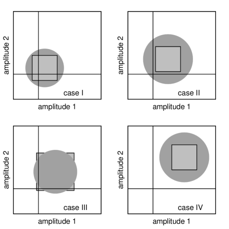
Figure 1: The illustration of various types of the interaction between the single-dimensional individual uncertainties (shown as a square error box) and the two-dimensional uncertainty domain (shown as a error circle). See text for the detailed discussion.

We give a graphical illustration of these types of outcomes in Fig. 1. In these plots we schematically show the uncertainty domains for the components amplitudes $K_{1}$ and $K_{2}$. For the sake of the simplicity, we adopt that the distributions of $K_{i}$ are uncorrelated and Gaussian, although this is far from the truth. In this illustration, to “detect” a single component or the couple means to ensure that a value $K_{i}=0$ for a given $K_{i}$ is outside of the relevant uncertainty domain. Notice that the uncertainty segments for a single $K_{i}$ are not just projections of the uncertainty circle for the couple $(K_{1},K_{2})$, because of the different number of the degrees of freedom. The sizes of the two-dimensional error ellipse and the error box inferred by the single-dimensional uncertainties is variable and depends on the distributions shape, on the dimnensionality of the problem, and on the ${\rm FAP}$ levels involved. The geometric relastionship between these regions may be different, although the diameter of the circle is always greater than the side of the box.

Of course, the cases II and III are mostly paradoxical. In the case II, the both variations are significant on themselves, but their joint significance is insufficient due to the dimensionality penalty. Here the circle encompasses the box entirely. In the case III, we can detect the components jointly, thanks to the accumulation of their contributions, but when we treat them individually, we deal with only a portion of this joint contribution, and this portion appears insignificant. Here the box and consequently the circle partly cover the axes $K_{i}=0$, but the origin $K_{1}=K_{2}=0$ is still outside of the circle.

One may think that these subtle geometric and probability effects are rather insignificant and might be just neglected in practice. This might seem so in the two-dimensional graphs shown above, but when the number of the frequency component grows, the role of these effects can become only more importaint. The dimensionality penalty increases, and the behaviour near the boundary of the uncertainty domain becomes decisive (recall that the most of the volume of a highly-dimensional ball resides near its surface, rather than in its core).

By this point, the reader might feel a bit confused, since the issue that we describe still may look rather fuzzy and foggy. Now he is prepared to look at it from yet another point of view. Foster (1996a, b) clearly explains how it is important to explicitly settle the null hypothesis of the signal detection task. This is the hypothesis that explains the data through a more simple model that does not contain the putative signal or some its portions. The main difficulty with this null hypothesis is that it frequently resides in the subconscious domain of a researcher’s mind, and is not explicitly realized even when it is pretty complicated. So, what null hypothesis we usually bear in mind when we claim “our dataset contains $n$ periodic components at the frequencies $f_{1},f_{2},\ldots,f_{n}$”?

A traditional detection algorithm, based on the sequential extraction of these components, assumes that the null hypothesis represents one of the following branches:

1. No signal at all, only a constant

2. The signal contains a single component $f_{1}$

3. Signal = component $f_{1}$ + component $f_{2}$ and no more

4. Signal = component $f_{1}$ + component $f_{2}$ + component $f_{3}$ and no more

   $\ldots$

5. Signal = sum of $n-1$ components, $f_{1}$ to $f_{n-1}$ and no more

However, this null hypothesis is obviously inappropriate, because it relies on a particular detection sequence: first extract $f_{1}$, secondly $f_{2}$, and so on. In such a case, our alternative hypothesis, which is a completion of the null one to the entire space of all admissible models, would embed the following special occurrences: “signal = a single component $f_{2}$”, “signal = component $f_{2}$ + component $f_{3}$ and no more”, and so on. These particular models are not the ones that we would like to have inside our alternative hypothesis, since they admit that some of the components that we claimed to reveal may not exist in some layout. Thus, even if we prove that this alternative hypothesis is true, this is not the initial proposition we aimed to prove. This occurs because our original null hypothesis listed above is incomplete. Note that the frequency values $f_{i}$ are not allowed to vary arbitrarily here, because they should always reside inside the relevant periodogram peaks, according to their detection sequence.

Since we want to prove that each of the components exists, we must adopt the complete null hypothesis, containing the following model branches:

1. No signal at all, only a constant

2. The signal contains a single component, any one of $f_{i}$

3. The signal is a sum of any two (and only two) components $f_{i}$ and $f_{j}$

4. The signal is a sum of any three (and only three) components $f_{i}$, $f_{j}$, $f_{k}$

   $\ldots$

5. Signal = sum of $n-1$ of the components that exclude any of $f_{i}$

This new null hypothesis takes into account the possiblity that e.g. the first extracted periodicity is due to the noise, while all others are still true. The previous null hypothesis undeservedly neglected such possibilities, disregarding their importance in the case when all relevant periodogram peaks have only a moderate significance, and no peak clearly dominates.

Our alternative hypothesis, that we want to prove, remains always the same: it states “the signal is indeed a sum of all $n$ detected components”. Different branches of our complete null hypothesis thus generate different test statistics. Following the same enumeration sequence as in the above list, they are:

1. The maximum of a single available $n$-frequency periodogram

2. $n$ maxima of the $(n-1)$-frequency periodograms (with one of $f_{i}$ moved to the base model)

3. $n(n-1)/2$ maxima of $(n-2)$-frequency periodograms (moving some pair of frequencies to the base model)

   $\ldots$

4. $n$ maxima of single-frequency periodograms, for which we have only one of $f_{i}$ in the signal model with the rest in the base one

From the computational point of view this task is much easier than it may seem. In practice, it is enough to maximize all these periodograms in only small vicinities of the estimated frequency values $f_{i}$. There is a little chance that the multi-frequency periodogram will show a remarkable peak at different frequencies. When the data sampling produce aliases, we may need to also scan the vicinities of all possible alias frequencies too (since we do not know in advance, which of the peaks are aliases). But in any way, we do not have to scan the entire multi-frequency space.

The number of the tests involving a $k$-component signal is $C_{n}^{k}$ (the binomial coefficient), hence their total number equals to $\sum_{k=0}^{n-1}C_{n}^{k}=2^{n}-1$. Each test generates its own value of the ${\rm FAP}$. In the frequentist framework that we adopt here, there is always some well-defined true signal model, determining which branch of the null hypothesis is real (when calculating the ${\rm FAP}$ we must not admit a thought that the null hypothesis itself might be wrong). Therefore, only one of the mentioned $2^{n}-1$ tests should be relevant. However, since we do not know which one that should be, we can select a worst-case result, i.e the maximum among these $2^{n}-1$ ${\rm FAP}$ values.

In pracice it is a frequent case when the periodograms contain more suspicious peaks than the ones that our sequential detection algorithm have extracted. Then it might be necessary to check whether these additional peak provide a better fit of the data in some other multiple combination. This is essentially what Foster (1995) calls the global CLEANest algorithm. This activity may result in a few of alternative sets of $f_{i}$. However, to rigorously prove the statistical significance of each such frequency set, i,e. to confirm a high confidence probability associated to the proposition “each of $f_{i}$ does exist” (conditionally to the selected rival configuration), we must ensure the individual significance of $f_{i}$ (as inferred by the single-frequency periodograms), as well as their significance in various multi-frequency combinations (within the adopted configuration of $f_{i}$). If just one of the relevant ${\rm FAP}$ values is too large, we have to admit that some of the extracted components still might be false positives.

We do not consider here the issue of distinguishing between different alternative sets of $f_{i}$, when these sets do not encompass each other (this may appear due to the aliases). This issue should be treated by means of different statistical tests that are designed to deal with non-nested models, see (Baluev, 2012).

There is also a minor matter that we need to highlight. Note that the single-frequency periodograms that provide some of the test statistics for verifying $f_{i}$, are the ones for testing $n$ signals against $n-1$ ones. These “verification periodograms” are different from the single-frequency periodograms that appear during the detection sequency, in which the hypothesis of $m$ signals is tested against the one with $m+1$ components, subsequently for $m=0,1,\ldots,n-1$ (this is what Foster (1995) calls as the SLICK spectrum). Only the last detection periodogram simultaneously belongs to the family of the verification ones. Obviously, the verification periodograms should be more reliable, because they likely involve a more adequate data model. They cannot be used at the detection stage, since we do not know in advance the number of the components to extract. We expect that these verification periodograms should typically generate higher peaks and concequently infer larger individual significances of $f_{i}$ than the detection periodograms (though we do not expect a big difference in the ${\rm FAP}$ as an abstract function of the maximum peak height $z$). This effect is nonetheless counterbalanced by the need to ensure that all multi-frequency combinations are also significant.

Therefore, to properly detect multiple periodic signals, the most of the significance tests that we apply, should be multi-frequency ones. Construction of a method that would allow to estimate such a joint multi-frequency significance is the main goal of our work.

4 Asymptotic significance levels

As it is well-known, the false alarm probability tied to an observed value of a signal detection statistic, is related to the distribution function of this quantity. When the frequencies $f_{i}$ are fixed (known a priori), such decisioning quantity would be just the value $z(\mn@boldsymbol{f})$. In this case, the model (2) would be entirely linear, and hence $2z(\mn@boldsymbol{f})$ would follow the chi-square distribution with $2n$ degrees of freedom. For $n=2$ this would imply ${\rm FAP}(z)=e^{-z}(z+1)$, for instance. However, in practice the frequencies $f_{i}$ are unknowns like $\mn@boldsymbol{\theta}$. Since $f_{i}$ are non-linear, the maximization of the periodogram $z(\mn@boldsymbol{f})$ is a non-trivial task, as well as the calculation of the necessary distribution function of its maximum peaks. To solve this task we will use the approach described by Baluev (2013). This approach is based on the generalized Rice method for random fields presented by Azaïs & Delmas (2002). The Rice method allows to obtan an estimation of the necessary false alarm probability in the following form:

$${\rm FAP}(z)\lesssim M(z),$$ (8)

where $z$ is the observed periodogram maximum, and $M(z)$ is an explicitly-defined function.

The high practical value of the estimation (8) is founded on the following things: (i) it usually has a good or at least satisfactory accuracy (in terms of the difference ${\rm FAP}-M$ or at least in terms of the $z$-level thresholds that are mapped to a given value of ${\rm FAP}(z)$ or $M(z)$); (ii) this accuracy increases for larger $z$, which has more practical importance, since in practice we need to have a good accuracy mainly for the small ${\rm FAP}$s; (iii) in the case when the deviation between $M(z)$ and ${\rm FAP}(z)$ is too large, the function $M(z)$ still serves as a majorant for ${\rm FAP}(z)$, guaranteeing that the number of false detection will never exceed the desired small level; (iv) the function $M(z)$ often can be approximated by a simple and accurate elementary formula.

For the Lomb-Scargle periodogram, for example, we obtained in (Baluev, 2008):

$${\rm FAP}(z)\lesssim M(z)\approx We^{-z}\sqrt{z}.$$ (9)

Now, let us first consider the more easy case of the double-frequency periodogram, and after that we proceed to dealing with the general multi-frequency periodogram.

Although the method in (Baluev, 2013) was originally designed to deal with a single (though non-sinusoidal) periodicity to detect, it still can be applied to a multi-frequency case with a help of a ruse. We cannot just directly substitute the model (2) in the formulae from (Baluev, 2013), because (2) contains $2n$ linear coefficients, instead of only a single signal amplitude, as we need for (Baluev, 2013). We need to transform (2) to an equivalent form, possibly looking more complicated, but containing only a single common amplitude parameter. For $n=2$, one way to do so leads to the following representation:

$$\mu=Kh,\quad h=\cos\alpha\cos(2\pi f_{1}t+\lambda_{1})+\sin\alpha\cos(2\pi f_{2}t+\lambda_{2}),$$ (10)

where $K$ is the mentioned single amplitude, and $h$ is a function of the time $t$ and of the five free parameters, including the new auxiliary non-linear parameter $\alpha$, responsible for the mixture of the two sinusoidal components.

When deriving our further results we will use the approximation of the ‘uniform phase coverage’ (UPC), as we called it in (Baluev, 2013). In this approximation, we neglect the quantities like

$$\langle t^{k}\cos\omega t\rangle,\quad\langle t^{k}\sin\omega t\rangle,$$ (11)

in comparison with $\langle|t|^{k}\rangle$ and similar quantities (in our case $k=0$, $1$, and $2$). This approximation is formally good only when $\omega$ is outside of a peak of the spectral window (the spectral leakage effect is negligible for a given $\omega$). However, as we have already discussed and demonstrated in many works (Baluev, 2008, 2009b, 2013) the presence of the spectral leakage itself does not yet significantly corrupt the quality of the final UPC approximation of the ${\rm FAP}$. This is because we should eventually perform an integration over a wide frequency range, and the anomalies generated by narrow peaks of the spectral window appear negligible after such an integration.

The UPC approximation basically enabled us just to drop all the terms of the type (11) anywhere we met them, leaving only the dominating terms $\langle t^{k}\rangle$.

According to Baluev (2013), first we need to construct from the model $h$ a normalized function $\psi$, such that $\langle\psi\rangle\equiv 0$, and $\langle\psi^{2}\rangle\equiv 1$. Since under the assumption of UPC we have $\langle h^{2}\rangle\approx 0$ already and $\langle h^{2}\rangle\approx\langle 1\rangle/2$, we can put $\psi\approx h\sqrt{2/\langle 1\rangle}$. Finally we need to evaluate the matrix $\textbf{{G}}=\langle\psi^{\prime}\otimes\psi^{\prime}\rangle$, based on the gradient $\psi^{\prime}\approx h^{\prime}\sqrt{2/\langle 1\rangle}$. The gradient of $h$ looks like:

$$h^{\prime}_{\alpha} =-\sin\alpha\cos(2\pi f_{1}t+\lambda_{1})+\cos\alpha\cos(2\pi f_{2}t+\lambda_{2}),$$

$$h^{\prime}_{\lambda_{1}} =-\cos\alpha\sin(2\pi f_{1}t+\lambda_{1}),$$

$$h^{\prime}_{f_{1}} =-2\pi t\cos\alpha\sin(2\pi f_{1}t+\lambda_{1}),$$

$$h^{\prime}_{\lambda_{2}} =-\sin\alpha\sin(2\pi f_{2}t+\lambda_{2}),$$

$$h^{\prime}_{f_{2}} =-2\pi t\sin\alpha\sin(2\pi f_{2}t+\lambda_{2}).$$ (12)

Using these formulae and UPC approximation, we obtain

G $$\approx\left(\begin{array}[]{@{}c@{\;}c@{\;}c@{\;}c@{\;}c@{}}1&0&0&0&0\\ 0&\cos^{2}\alpha&2\pi\bar{t}\cos^{2}\alpha&0&0\\ 0&2\pi\bar{t}\cos^{2}\alpha&4\pi^{2}\bar{t^{2}}\cos^{2}\alpha&0&0\\ 0&0&0&\sin^{2}\alpha&2\pi\bar{t}\sin^{2}\alpha\\ 0&0&0&2\pi\bar{t}\sin^{2}\alpha&4\pi^{2}\bar{t^{2}}\sin^{2}\alpha\\ \end{array}\right),$$ (18)

$$\overline{t^{k}}=\langle t^{k}\rangle/\langle 1\rangle,$$ (19)

which also implies

$$\sqrt{\det\textbf{{G}}}\approx\frac{\pi}{4}T_{\mathrm{eff}}^{2}\sin^{2}2\alpha,\qquad T_{\mathrm{eff}}=\sqrt{4\pi(\overline{t^{2}}-{\overline{t}}^{2})}.$$ (20)

We note that the quantity $T_{\mathrm{eff}}$, emerging here, is the effective length of the time series that was first introduced in (Baluev, 2008).

The quantity $\sqrt{\det\textbf{{G}}}$ should now be integrated over the space of all five free parameters $\alpha,\lambda_{i},f_{i}$ to obtain the final result:

$${\rm FAP}(z) \lesssim M(z)\simeq Ae^{-z}z^{d/2-1},$$

$$A =\frac{1}{2\pi^{d/2}}\int\sqrt{\det\textbf{{G}}}\;df_{1}df_{2}d\lambda_{1}d\lambda_{2}d\alpha,$$ (21)

where $d$ — the number of free model parameters — is now equal to $6$.

Here we should take care of one subtle thing: over what exactly domain we must do the integration? We must take into account that the mentioned parameters of the signal satisfy a few relations of equivalence. Namely, the following six vectors of the parameters

$$\begin{array}[]{@{\{}rrrrrr@{\},}}K,&\alpha,&\lambda_{1},&f_{1},&\lambda_{2},&f_{2}\\ -K,&\alpha,&\lambda_{1}+\pi,&f_{1},&\lambda_{2}+\pi,&f_{2}\\ -K,&\alpha+\pi,&\lambda_{1},&f_{1},&\lambda_{2},&f_{2}\\ K,&\pi-\alpha,&\lambda_{1}+\pi,&f_{1},&\lambda_{2},&f_{2}\\ K,&-\alpha,&\lambda_{1},&f_{1},&\lambda_{2}+\pi,&f_{2}\\ K,&\frac{\pi}{2}-\alpha,&\lambda_{2},&f_{2},&\lambda_{1},&f_{1}\\ \end{array}$$ (22)

all describe the same signal (10). To encompass all possible signals inside a frequency range $[f_{\mathrm{min}},f_{\mathrm{max}}]$, simultaneously throwing away all the duplicates, we may consider the following domain:

$$K\geq 0,\quad 0\leq\alpha\leq\frac{\pi}{4},\quad 0\leq\lambda_{i}\leq 2\pi,\quad f_{\mathrm{min}}\leq f_{i}\leq f_{\mathrm{max}}.$$ (23)

Notice that the condition $K\geq 0$ is exactly the one required in (Baluev, 2013) for (21) to be valid (otherwise $A$ should be doubled). The condition $\alpha\leq\pi/4$ appears because due to the last equivalence of (22) the replacement $\alpha\mapsto\pi/2-\alpha$ would just swap the signal components with each other, keeping the sum intact. Performing the integration over the domain described, we eventually obtain

$${\rm FAP}(z)\lesssim M(z)\approx\frac{\pi}{16}W^{2}e^{-z}z^{2},\quad W=T_{\mathrm{eff}}(f_{\mathrm{max}}-f_{\mathrm{min}}).$$ (24)

The formula (24) is valid for the case when the frequencies $f_{i}$ belong to the same range. Sometimes we may have some prior information that would imply different ranges for $f_{1}$ and $f_{2}$. In the case when these ranges do not intersect, we should extend the integration domain from $0\leq\alpha\leq\pi/4$ to $0\leq\alpha\leq\pi/2$, because now the frequency components are not freely swappable and the last equivalence of (22) is no longer valid. This will double the result. In the most general case, when the frequency ranges are partially intersecting, we may write down:

$${\rm FAP}(z)\lesssim M(z)\approx\frac{\pi}{16}(2W_{1}W_{2}-W_{12}^{2})e^{-z}z^{2},$$ (25)

where $W_{1}$ and $W_{2}$ are associated with the frequency ranges of $f_{1}$ and $f_{2}$, while $W_{12}$ is related to their common intersection.

The formulae for $M(z)$ in (21) and, consequently (24) and (25), make some additional approximating assumptions that we still need to discuss. The first thing it neglects is the effect of the domain (23) boundary, which importance was described in (Baluev, 2013). In the case of the double-frequency periodogram, the boundary sides $f_{1}=f_{\mathrm{min},\mathrm{max}}$ and $f_{2}=f_{\mathrm{min},\mathrm{max}}$ generate an extra term in (24) of the order of $\sim We^{-z}z^{3/2}$, and an extra term for the vertices of the relevant frequency box would be $\sim e^{-z}z$. The non-frequency parameters $\lambda_{i}$ and $\alpha$, thanks to their periodicity, do not generate any boundary effects. Anyway, all these extra terms are negligible, because the value of $W$ in practice is typically large or very large ($\sim 100$ or $\sim 1000$ or even more). The relevant correction to (24) would have a very small relative magnitude of $\sim 1/(W\sqrt{z})$ and $\sim 1/(zW^{2})$. No doubts, it can be safely neglected in practice.

The other small terms that were dropped off in (21), have the relative magnitude of $\sim 1/z$ and $\sim 1/z^{2}$. As we have already discussed in (Baluev, 2013), these terms are usually very difficult to evaluate, because they involve manipulations already with second-order dervatives of $\psi$, combined in tensors of order $4$ and dimension $n$. In our case, it is a $5\times 5\times 5\times 5$ tensor, for instance. These terms are also expected to be negligible, because we are usually interested in large values of $z$: typically, when $z$ is smaller than $10$, the signal is very uncertain, and the associated false alarm probability is large, so we just have no real need to know this probability with a good precision. However, in the particular case of the double-frequency periodogram, we were able to rigorously evaluate these terms, rather than just to blindly neglect them. This appeared possible because of the simplicity of the signal model. According to our results, the corrected general expression (25) looks like

$${\rm FAP}(z) \lesssim M(z)\approx e^{-z}\Bigg{[}\frac{\pi}{16}(2W_{1}W_{2}-W_{12}^{2})(z^{2}+2z+2)-$$

$$-W_{1}W_{2}\left(z+\frac{1}{2}\right)\Bigg{]}.$$ (26)

In the case of the same frequency range for the both frequencies ($W_{1}=W_{2}=W_{12}=W$) we therefore have

$${\rm FAP}(z)\lesssim M(z)\approx W^{2}e^{-z}\left[\frac{\pi}{16}z^{2}+\left(\frac{\pi}{8}-1\right)z+\frac{\pi-4}{8}\right].$$ (27)

We do not give the detailed derivation of (26) and (27), because it still appeared very complicated. We only mention that we used the general formulae of Proposition b of Theorem 1 by Azaïs & Delmas (2002). Some extra discussion can be also found in (Baluev, 2013). Actually, we wrote down these refined results here only to demonstrate below that their difference from (25) and (24) is negligible.

Let us now consider the general multi-frequency case. Now we may put

$$\mu=Kh,\quad h=\sum_{k=1}^{n}\nu_{k}\cos(2\pi f_{k}t+\lambda_{k}),$$ (28)

where $\nu_{k}$ are components of a unit vector $\mn@boldsymbol{\nu}$ parameterized by $n-1$ spherical angles forming another vector $\mn@boldsymbol{\alpha}$. Now the gradient of $h$ looks like

$$h^{\prime}_{\mn@boldsymbol{\alpha}} =\sum_{k=1}^{n}\frac{\partial\nu_{k}}{\partial\mn@boldsymbol{\alpha}}\cos(2\pi f_{k}t+\lambda_{k}),$$

$$h^{\prime}_{\lambda_{k}} =-\nu_{k}\sin(2\pi f_{k}t+\lambda_{k}),$$

$$h^{\prime}_{f_{k}} =-2\pi t\nu_{k}\sin(2\pi f_{k}t+\lambda_{k}).$$ (29)

These expressions allow us to write down the matrix G very similarly to the double-frequency case; the necessary determinant can be then expressed as

$$\sqrt{\det\textbf{{G}}}\approx\pi^{n/2}T_{\mathrm{eff}}^{n}(\nu_{1}\nu_{2}\ldots\nu_{n})^{2}\sqrt{\det\left(\frac{\partial\mn@boldsymbol{\nu}}{\partial\mn@boldsymbol{\alpha}}^{\rm T}\frac{\partial\mn@boldsymbol{\nu}}{\partial\mn@boldsymbol{\alpha}}\right)}$$ (30)

The last multiplier in this expression, containing the gradient of $\mn@boldsymbol{\nu}$ over $\mn@boldsymbol{\alpha}$, is rather unpleasant and needs some simplification. Let us define an auxiliary square matrix $\textbf{{R}}=(\mn@boldsymbol{\nu},\partial\mn@boldsymbol{\nu}/\partial\mn@boldsymbol{\alpha})$, and try to find its squared determinant:

$$(\det\textbf{{R}})^{2}=\det(\textbf{{R}}^{\rm T}\textbf{{R}})=\det\left(\begin{array}[]{@{}cc@{}}\mn@boldsymbol{\nu}^{\rm T}\mn@boldsymbol{\nu}&\mn@boldsymbol{\nu}^{\rm T}\frac{\partial\mn@boldsymbol{\nu}}{\partial\mn@boldsymbol{\alpha}}\\ \frac{\partial\mn@boldsymbol{\nu}}{\partial\mn@boldsymbol{\alpha}}^{\rm T}\mn@boldsymbol{\nu}&\frac{\partial\mn@boldsymbol{\nu}}{\partial\mn@boldsymbol{\alpha}}^{\rm T}\frac{\partial\mn@boldsymbol{\nu}}{\partial\mn@boldsymbol{\alpha}}\\ \end{array}\right).$$ (31)

Since the identity $\mn@boldsymbol{\nu}^{2}\equiv 1$ holds true for every $\mn@boldsymbol{\alpha}$, the off-diagonal elements of the last matrix in (31) are zero, the top-left element is unit, and we finally obtain

$$\sqrt{\det\textbf{{G}}}\approx\pi^{n/2}T_{\mathrm{eff}}^{n}(\nu_{1}\nu_{2}\ldots\nu_{n})^{2}\left|\det\left(\mn@boldsymbol{\nu},\frac{\partial\mn@boldsymbol{\nu}}{\partial\mn@boldsymbol{\alpha}}\right)\right|.$$ (32)

The last determinant basically represents the Jacobian of the transition from the Cartesian to the spherical coordinate system, i.e. from $\mn@boldsymbol{x}=r\mn@boldsymbol{\nu}$ to the pair $(r,\mn@boldsymbol{\nu})$.

Let us recall the formulae of the multi-dimensional spherical parametrization:

$$\nu_{1} =\cos\alpha_{1},$$

$$\nu_{2} =\sin\alpha_{1}\cos\alpha_{2},$$

$$\nu_{3} =\sin\alpha_{1}\sin\alpha_{2}\cos\alpha_{3},$$

$$\ldots$$

$$\nu_{n-1} =\sin\alpha_{1}\sin\alpha_{2}\ldots\sin\alpha_{n-2}\cos\alpha_{n-1},$$

$$\nu_{n} =\sin\alpha_{1}\sin\alpha_{2}\ldots\sin\alpha_{n-2}\sin\alpha_{n-1},$$ (33)

where all $\alpha_{i}$ except for the last one, should in general reside in the segment $[0,\pi]$, and $\alpha_{n-1}$ is allowed to vary inside $[0,2\pi]$.

With these formulae we can rewrite (32), after rather long but straightforward manipulations, in a detailed form:

$$\sqrt{\det\textbf{{G}}}\approx\pi^{n/2}T_{\mathrm{eff}}^{n}\prod_{k=1}^{n-1}\sin^{3k-1}\alpha_{n-k}\cos^{2}\alpha_{n-k}.$$ (34)

Again the issue arises, what integration domain we should adopt for (34)? This should be the largest possible domain that still does not contain any equivalent pairs of points (describing the same signal). Now it is easier to consider the case when the frequencies $f_{i}$ all belong to different segments, and these segments do not intersect with each other. Then we may adopt the domain

$$K\geq 0,\quad 0\leq\alpha_{i}\leq\frac{\pi}{2},\quad 0\leq\lambda_{i}\leq 2\pi,\quad f_{i,\mathrm{min}}\leq f_{i}\leq f_{i,\mathrm{max}}.$$ (35)

The condition $\alpha_{i}\in[0,\pi/2]$ appeared because the signs of individual terms in (28) are managed by the longitudes $\lambda_{i}$, while all $\nu_{i}$ must then be positive to get rid of duplicate signals in the domain.

Substituting all necessary quantities to (21) and integrating, we obtain

$${\rm FAP}(z) \lesssim M(z)\simeq A_{n}e^{-z}z^{3n/2-1},$$

$$A_{n} =W_{1}W_{2}\ldots W_{n}I_{1}I_{2}\ldots I_{n-1},$$

$$I_{k} =2\int\limits_{0}^{\pi/2}\sin^{3k-1}\alpha\,\cos^{2}\alpha\,d\alpha=B\left(\frac{3k}{2},\frac{3}{2}\right).$$ (36)

For the more practical case, in which there is a single common frequency segment $W$, it is rather difficult to define the necessary integration domain for $\alpha_{i}$. Instead, let us try to correct the formula (36). What is the underlying reason making the normalization of the ${\rm FAP}$ different for the cases of the shared and independent frequency segments? Of course, this is the symmetry property of the multi-frequency periodogram. For the double-frequency periodogram the obvious identity $z(f_{1},f_{2})=z(f_{2},f_{1})$ implies that only a half of the frequency square $W\times W$ is informational; another half is just a mirror copy. This halves the resulting ${\rm FAP}$ value — compare (24) and (25) with $W_{12}=0$. In the case of the general multi-frequency periodogram only a single $n$-simplex inside the entire frequency cube is informational. Since the volume of this simplex constitutes $1/n!$ fraction of the cube volume, we have for this case

$${\rm FAP}(z) \lesssim M(z)\simeq\tilde{A}_{n}e^{-z}z^{3n/2-1},$$

$$\tilde{A}_{n}=\frac{W^{n}}{n!}I_{1}I_{2}\ldots I_{n-1}.$$ (37)

From this general approximation we can easily reconstruct the ${\rm FAP}$ formulae for the Lomb-Scargle periodogram (9) and for the double-frequency periodogram (24).

We do not consider here the most general case when the frequency segments are different but may have common parts.

5 Some further extensions

The multi-frequency periodogram defined in (6) assumes the empty null hypothesis: the input data are expected to represent the pure noise or the pure noise plus a signal with no even an offset. Therefore, another possible way to generalize the multi-frequency periodogram is to consider some non-trivial base models describing an expected underlying variation (the non-trivial null hypothesis). In practice there should be at least a free constant term in the null hypothesis, because the data $x_{i}$ almost always have an arbitrary offset to be determined from the data.

It is already clearly demonstrated in the literature that this is a bad practice to just pre-center the input time series and then pass the residuals to the LS periodogram (Cumming et al., 1999). Instead, we must honestly perform the linear regression under the null hypothesis (“data are equal to an unknown constant”), under the alternative one (“the data are equal to a constant plus the putative signal”) and evaluate the inferred test statistic. For the $n=1$ (Lomb-Scargle) case this was essentially done by Ferraz-Mello (1981), who defined the so-called Date-Compensated Discrete Fourier Transform, DCDFT. This periodogram is known rather well already, though in the literature it is referred to under different names; e.g. it is called as just “the generalized periodogram” by Zechmeister & Kürster (2009). We prefer an intuitive and concise name “the floating-mean periodogram”, given by Cumming et al. (1999).

Cumming et al. (1999) also suggested to extend the floating-mean periodogram further, taking into account an arbitrary linear or a quadratic trend in the data. Moreover, it is quite easy to construct a generalized periodogram with an arbitrary multi-parametric linear model (e.g. a polynomial trend) of the underlying variation (Baluev, 2008). In this case, the definition (6) must also involve the linear regression made for this non-trivial base model. We should replace (6) by

$$z(\mn@boldsymbol{f})=\frac{1}{2}\left(\min_{\mn@boldsymbol{\theta}_{\mathcal{H}}}\chi^{2}_{\mathcal{H}}(\mn@boldsymbol{\theta}_{\mathcal{H}})-\min_{\mn@boldsymbol{\theta}_{\mathcal{K}}}\chi^{2}_{\mathcal{K}}(\mn@boldsymbol{\theta}_{\mathcal{K}},\mn@boldsymbol{f})\right),$$ (38)

where $\chi^{2}_{\mathcal{H},K}$ are the $\chi^{2}$ goodness-of-fit functions (4), now corresponding to either null ($\mathcal{H}$) or the alternative ($\mathcal{K}$) models. Previously, for an empty $\mathcal{H}$, we had just $\chi_{\mathcal{H}}^{2}\equiv\langle x^{2}\rangle$.

When the underlying variation is modelled by a low-order polynomial, the theory of significance levels from Section 4 remains practically unchanged, because under the assumption of UPC the powers of time, $t^{k}$, appear orthogonal to the sine and cosine functions, since during the calculation of the extreme-value distribution we anyway neglect the terms like (11). For the extensions of the Lomb-Scragle periodogram we checked it in (Baluev, 2008, 2009b), and below we verify this for the double-frequency periodogram too, using the Monte Carlo simulations.

In the Sections 2 and 4 we only considered the case when $\sigma_{i}$ are known precisely. In practice we usually do not know them with good accuracy. Usually only the weights $w_{i}$ of the observations are known, while the full variances are determined through $w_{i}$ as $\sigma_{i}^{2}=\kappa/w_{i}$, where $\kappa$ is an extra unknown parameter. In this case we need to introduce some normalization of the periodogram, since the value of $\chi^{2}$ is now proportional to the unknown multiplier $\kappa$. We recommend to use in this case a multi-frequency analog of the periodogram $z_{3}$ from (Baluev, 2008). We can define it here as

$$z_{3}(\mn@boldsymbol{f})=-\left(\frac{N_{\mathcal{H}}}{2}-n\right)\log\left(1-\frac{2z(\mn@boldsymbol{f})}{\min\chi^{2}_{\mathcal{H}}}\right),$$ (39)

where $N_{\mathcal{H}}=N-\dim\mn@boldsymbol{\theta}_{\mathcal{H}}$.

This periodogram is related to the likelihood ratio statistic, and for large $N$ its distributions (including the distribution of the maximum) are asymptotically the same as the ones of the $\chi^{2}$-statistic $z(\mn@boldsymbol{f})$. We have already discussed this issue in (Baluev, 2009a, 2013). For the single-frequency variant of $z_{3}$ the reader may find more accurate expression of the type (8), which do not rely on the $N\to\infty$ asymptotics, in (Baluev, 2008). It is easy to ensure that they are indeed asymptotically equivalent to the similar expressions for $z$, if the extra condition $z,z_{3}\ll N$ is also satisfied. The principal nature of this condition is explained in (Baluev, 2009a), and we believe that it should be valid in the case of the multi-frequency periodogram too. Unfortunately, at present we cannot generalize the more accurate formula for $M(z_{3})$ from (Baluev, 2008) to the multi-frequency case, because this would need the generalized Rice method for non-Gaussian random fields, which is to our awareness still poorly developed. At present we have to approximate the function $M(z_{3})$ by its analog $M(z)$, as we have just described. Notice that the ${\rm FAP}$ will be anyway extremely small for the values of $z$ or $z_{3}$ as large as $N$, so in practice the need to satisfy an extra condition like $z\ll N$ should not produce any significant side effects. At least, this is well confirmed by the numerical simulations discussed below.

Finally, we may consider a weakly non-linear base model, which may include e.g. some previously detected periodicities. These periodograms are extensively referred to in Section 3. The base frequencies are formally non-linear parameters, but they are linearizable, since once the periodicity is extracted, its frequency always resides within a narrow periodogram peak. For these periodograms the argumentation of the above paragraph applies qualitatively: the ${\rm FAP}$ formulae of Section 4 should work in the asymptotic sense $N\to\infty$. However, we should realize that in concrete practical cases with a concrete $N$ these ${\rm FAP}$ approximation may fail sometimes, e.g. after we have already extracted a large number of the signal components. This issue is something that we leave for future work.

6 Simulations

We have done some numerical simulations to check our analytical results. In these simulations, we used the double-frequency periodogram with a free constant term in the base model (a double-frequency analog of the generalized floating-mean periodogram by Ferraz-Mello (1981) and Zechmeister & Kürster (2009)). We considered both the case with known $\sigma_{i}$ and the case when $\sigma_{i}$ contain an unknown factor. In all the cases we deal with a single range for the both frequencies $f_{i}$ (meaning that $W_{1}=W_{2}=W_{12}=W$). The main results are shown in Fig. 2, where for $W\approx 100$ and different time series we plot the simulated ${\rm FAP}$ curves together with the analytic approximation (24) and its refined version (26). As for the Lomb-Scargle periodogram, the quality of our analytic formulae is the best for an even time series, and degrades for a time series with strong aliasing. However, our estimation always consitutes an upper limits on the ${\rm FAP}$. We can always be pretty sure that if we got the estimation of, e.g. $M(z)=1\%$, the actual value of ${\rm FAP}$ may be almost the same or smaller than this value. This means that the use of $M(z)$ from (24) instead of ${\rm FAP}$ does not increase the number of false alarms above the desired level.

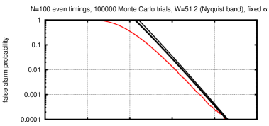
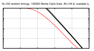
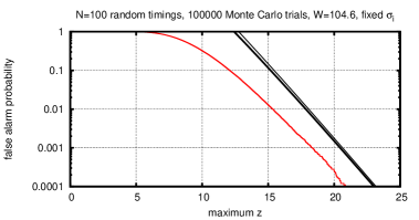
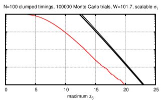
Figure 2: The graphs comparing the analytic ${\rm FAP}$ estimations (24) (thick solid curves) and (27) (thin solid curves) and the simulated ${\rm FAP}$ (noisy thin curves, red in the electronic version). The panels to the left correspond to the cases with the noise uncertainties $\sigma_{i}$ are known a priori; the ones to the right are for the fixed-weights model with $\sigma_{i}^{2}\propto 1/w_{i}$. In the case of “clumped timings” (right-bottom panel) the $N=100$ points of the data were equally split in $10$ equidistant groups with $90\%$ time gaps between them. This implies a very strong aliasing, which invalidates our ${\rm FAP}$ formula as an approximation but does not break its upper limit property.

A bad side effect of possible deviation between $M$ and ${\rm FAP}$ is the increase of the detection threshold. However, in the worst case of Fig. 2 this increase constitutes the relatitve magnitude of $\sim 1/3$, which is not catastrophic at all.

It may be noted that with the increase of $W$ to a more practical level of $\sim 1000$, the precision of our ${\rm FAP}$ estimate gets even better (Fig. 3). We believe this is because larger value of $W$ makes the signal/noise threshold to move to a higher $z$-level, and the Rice method becomes more accurate for $z\to\infty$, since it has an asymptotic nature.

At last, we can conclude, that the refined formula (26) does not have any practical advatage with respect to the original more simple expressions (25) and (24). As we expected, only the leading $z^{2}$ term is important in (26), and the others are neglectable. As usually, the main source of the error of our approach is the intrinsic error of the Rice method (the difference between $M(z)$ and ${\rm FAP}(z)$), rather than the inaccuracy of the approximated $M(z)$.

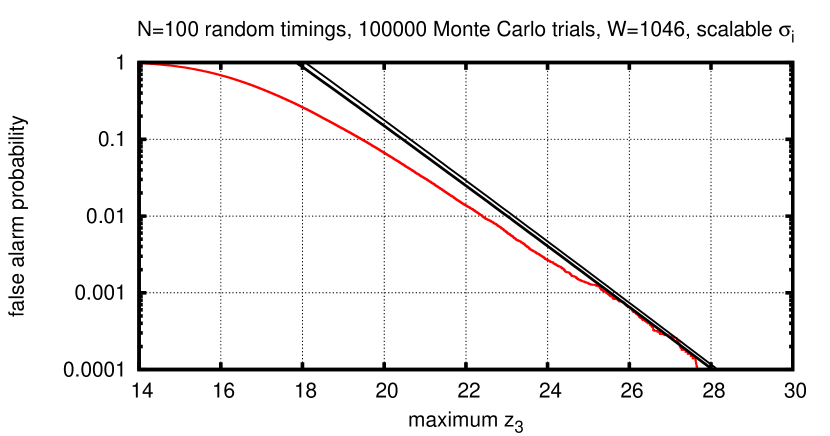
Figure 3: Same as the right-top panel of Fig. 2, but for a much wider frequency range. Notice that the increase of $W$ made our analytic estimations more accurate.

Performing similar Monte Carlo simulations for a multi-frequency periodogram with $n>2$ is not feasible due to the huge computational demands. Nonetheless, it would not be comfortable just to leave the multi-frequency ${\rm FAP}$ approximation from Section 4 without any numerical verification at all, because the relevant math manipulations were not trivial. At least, we should ensure that that these ${\rm FAP}$ formulae do not hide e.g. a error in the coefficient.

The direct maximization of $z(\mn@boldsymbol{f})$ is a computation-heavy procedure, but in some simple cases it can be dramatically simplified. Namely, when the observations are distributed uniformly in time (strictly evenly or randomly with uniform distribution), we can apply the UPC approximation to the periodogram itself, rather than only to its ${\rm FAP}$ approximation. In this case the sinusoidal terms in (2) appear practically orthogonal to each other. Then, considering that $\sigma_{i}$ are known, the following approximate expansion appears:

$$z(\mn@boldsymbol{f})\approx z_{\rm sf}(f_{1})+z_{\rm sf}(f_{2})+\ldots+z_{\rm sf}(f_{n}).$$ (40)

Here the function $z_{\rm sf}$ is the relevant single-frequency periodogram (actually, its Ferraz-Mello’s version in our case). This expansion is valid everywhere except for the neighbourhoods of the diagonals $f_{i}=f_{j}$.

Obviously, the maximum of the sum in (40) is achieved if and only if each of $f_{i}$ corresponds to a peak of $z_{\rm sf}(f)$. However, we cannot just select the absolute maximum of $z_{\rm sf}(f)$ at some $f=f^{*}$ and claim that the global maximum of $z(\mn@boldsymbol{f})$ is at $f_{i}=f^{*}$ and is equal to $n\max z_{\rm sf}$. This would imply that all $f_{i}$ are equal to each other, which invalidates (40). Instead of this, we should locate $n$ different tallest peaks of $z_{\rm sf}(f)$ and sum them up to approximate the global maximum of $z(\mn@boldsymbol{f})$.

This approximation allows us to dramatically speed up our Monte Carlo simulations, although now we can only deal with the cases that are free of spectral leakage. Instead of scanning the multi-dimensional frequency grid, it is enough to evaluate the single-frequency periodogram.

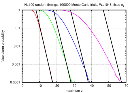
Figure 4: The simulated ${\rm FAP}$ curves for the multi-frequency periodograms obtained using the approximation (40), and the theoretic ${\rm FAP}$ estimations (37). The adopted number of the frequency components was $n=1,2,3$, and $5$ (from left to right).

The results are shown in Fig. 4. We may notice that the simulated ${\rm FAP}$ curves slightly break the inequality of (37) in the range below the level of $10^{-3}$. We believe this indicates the inaccuracy of the expansion (40) rather then the actual breaking of (37). This is because in the previous simulation of Fig. 3 the double-frequency ${\rm FAP}$ did not exceed the analytic estimation, while in Fig. 4 it does. Taking into account the inaccuracy of (40) and Monte Carlo uncertainties, our conclusion is that the analytic estimation (37) does not hide an obvious math error at least.

7 Detection sensitivity

It is interesting to investigate the detection sensitivity of the multi-frequency statistic, comparing it with the classic single-frequency one. We will do this in a simplified framework, in terms of the ${\rm FAP}$ estimations (24) and (9). We consider only the case $n=2$. According to the argumentation of Section 3, we must evaluate in this case three periodograms: two single-frequency residual periodograms (Foster’s SLICK periodograms computed assuming that one of the periodicities is in the base model) and the only available double-frequency periodogram.

Let us first assume that amplitudes of the periodic components are equal. Then, in a rough approximation (discarding the aliasing effects), the maximum values of the single-frequency periodograms are equal to each other, and according to (40), the maximum the double-frequency periodogram is roughly twice the maximum of the single-frequency ones. This means that we should compare the values of (9) with (24), substituting some $z$ in the first and $2z$ in the second. Notice that the plain Lomb-Scargle periodogram of the raw data is equal, in this approximation, to the sum of the individual single-frequency periodograms mentioned above. Therefore, it will posess two distinct peaks at their relevant frequencies, both having approximately the same height of $z$.

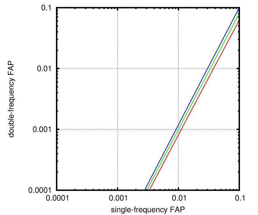
Figure 5: Comparison of the detection efficency of the single- and double- frequency periodograms in terms of the analytic ${\rm FAP}$ estimations from (9) and (24). The three plotted curves correspond to $W=100$, $1000$, and $10000$. The actual signal is assumed to involve two periodicities of the same amplitude, so the maximum value of the single-frequency periodogram is roughly half of that of the double-frequency one.

We plot the relevant ${\rm FAP}$ comparison graphs in Fig. 5, for $W=100$, $1000$, and $10000$. We may notice two things: the double-frequency periodogram appears in this case definitely superior over the single-frequency one in terms of the sensitivity, and this advantage is almost independent of $W$. This means that when our periodic components have equal amplitudes, it is unlikely that the double-frequency periodogram may disprove the single-frequency detections.

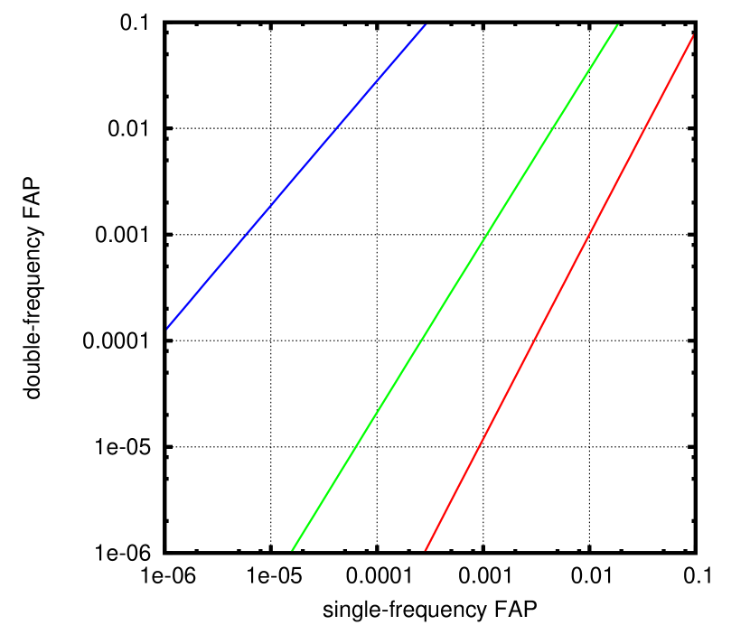
Figure 6: Similar to Fig. 5, but now we fix $W=1000$ and vary the amplitude ratio of the sinusoidal components: $1\!:\!1$, $1.2\!:\!1$, and $2\!:\!1$ (curves from right to left).

When we consider the cases of unequal amplitude ratio (Fig. 6), we can find that it affects crucially the sensitivity of the double-frequency periodogram relatively to the single-frequency one. For the amplitude ratio $1.2$ the sensitivities become roughly similar, and after that the double-frequency ${\rm FAP}$ becomes much larger than the single-frequency one. Therefore, in the more frequent cases with unequal amplitudes, the extra statistical verification by the double-frequency periodogram is mandatory, since it may easily disprove our single-frequency detections.

However, we may notice that in terms of the detection thresholds (critical $z$ levels) the difference between the single- and double-frequency periodograms is not that huge as it may seem when we compare ${\rm FAP}$s in Fig. 6. From (9) and (24) we conclude that the difference between the $z$ levels is roughly the logarithm of the relevant ${\rm FAP}$ ratio.

8 A double-frequency example

In the above sections, the reader may become convinced that we preach a single purpose of the multi-frequency periodogram: disappoint a hasty person who claimed a detection of several periods too soon. This not the only purpose, of course. Let us provide some demonstration of how the double-frequency periodogram may work in a constructive rather than destructive manner. We consider the following model example. The $N=150$ data points are clumped in $5$ groups (each contains $30$ randomly distributed points) separated by gaps. The gaps cover $43\%$ of each such “data+gap” chunk. The data are noisless and contain only a signal, which is a sum of two cosinusoidal components with $f_{1}=0.9$ Hz and $f_{2}=1.1$ Hz and equal amplitudes. The phases of the components are $0^{\circ}$ and $145^{\circ}$.

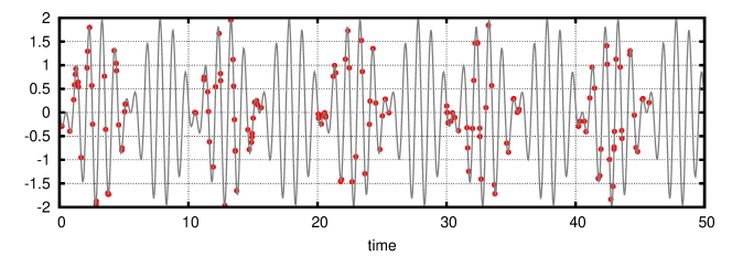
Figure 7: The signal and data of the model example of Section 8. The signal contains two periodic components which generate the beating, and the dataset is such that only each odd beating cycle is sampled (see text for the detailed description). The noise is absent.

This signal represents a beating process shown in Fig. 7. We can see that the gaps in the data are such that only each odd beating cycle is sampled. The DCDFT periodogram of these data shows no much difference with the case of a single sinusoid at $f=1.0$ Hz (Fig. 8). In practice we would be unable to distinguish such single- and double-frequency case. The only difference is that the side peaks in the double-frequency case are larger than for the single-frequency one. However, in practice this would just make us to think that the spectral leakage is a bit stronger than it actually is. Therefore, the we are unable to find a correct model for the signal in Fig. 7: the single-frequency periodogram would direct us to a wrong way from the very beginning stage of the analysis.

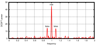
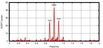
Figure 8: The Lomb-Scargle periodograms of two synthetic datasets: of the one shown in Fig. 8 with two periodicities at $0.9$ Hz and $1.1$ Hz (right graph), and of a similar one containing only a single periodicity at $1.0$ Hz (left graph). The time series involves periodic gaps generating an aliasing frequency of $0.1$ Hz (see text for the detailed description). The noise is absent.

However, armed with the double-frequency periodogram, we can find the correct solution of the problem immediately. As we can see in Fig. 9, this periodogram reveals the correct period pair for the double-frequency signal, and simultaneously it does not generate any undesired additional periods for the single-period data.

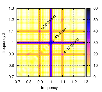
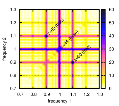
Figure 9: The double-frequency periodograms plotted for the same datasets as in Fig. 8. We label the highest peaks with the corresponding maximum periodogram values.

Of course, in practice the success of the analysis would also depend on the signal/noise ratio, but the Lomb-Scargle periodogram failed already for entirely noiseless data that we have just considered.

Our general conclusion is that the double- and multi-frequency periodograms may appear rather useful in certain especially difficult time-series analysis tasks. They are able to reveal correct periodic solutions in the cases when single-frequency periodograms fail.

9 Conclusions

On itself, it is usually quite easy to invent a sophisticated periodogram to satisfy the demands of some specific data-analysis task. For example, the multi-frequency periodogram that we considered here was known for almost two decades already. One of the principal obstacles that put a strict limitation on the practical use of such periodograms is the need of a simultaneously rigorous, general, and computationally efficient approach to evaluate the significance levels associated with these new periodograms. Even for the classic Lomb-Scargle periodogram the evaluation of these significance levels represented a substantial difficulty over decades.

We believe that the ${\rm FAP}$ estimation approach based on the generalized Rice method, that we are using extensively during last 5 years, satisfies all these requests. It inherits the generality and rigorous basis of the Rice method. Also, it often leads to entirely analytic and self-closed results that work according to a simple principle “just substitute”.

The importance of the detection significance levels for the multi-frequency periodogram is even further emphasized, because it is not just some fancy multi-frequency periodogram that we may use or may refuse to use. As we have discussed, the need to assess the multi-frequency ${\rm FAP}$ still persists even when we detect periodicities in a sequential single-frequency manner. If we wish to have nothing common with any multi-frequency periodograms, we may produce an increased number of false detections.

We would like draw some more attention to the comparison of the Lomb-Scargle ${\rm FAP}$ formulae (9) with e.g. its double-frequency analog (24). Remarkably, they looks rather simialar to each other. In fact, we could easily guess the correct powers of $W$ and of $z$ in (24), based on (9), even without any sophisticated calculations, just by taking into account the increase of the number of the free parameters of the signal. However, it would be impossible to guess the non-trivial and important coefficient of $\pi/16\approx 1/5$. It could be derived only by means of a rigorous application of the generalized Rice method, as we have done here.

So far in the paper, we paid little attention to the task of practical computation and maximization of the multi-frequency periodogram. Obviously, this may constitute a challenge already for $n\geq 3$. In the next Paper II, an efficient parallellized computation algorithm is to be presented. The beta version of this algorithm is already available for download at http://sourceforge.net/projects/fredec/, although with only a little documentation until Paper II.

References

- Azaïs & Delmas (2002) Azaïs J.-M., Delmas C., 2002, Extremes, 5, 181
- Baluev (2008) Baluev R. V., 2008, MNRAS, 385, 1279
- Baluev (2009a) Baluev R. V., 2009a, MNRAS, 393, 969
- Baluev (2009b) Baluev R. V., 2009b, MNRAS, 395, 1541
- Baluev (2012) Baluev R. V., 2012, MNRAS, 422, 2372
- Baluev (2013) Baluev R. V., 2013, MNRAS, 431, 1167
- Cumming et al. (1999) Cumming A., Marcy G. W., Butler R. P., 1999, ApJ, 526, 890
- Ferraz-Mello (1981) Ferraz-Mello S., 1981, AJ, 86, 619
- Foster (1995) Foster G., 1995, AJ, 109, 1889
- Foster (1996a) Foster G., 1996a, AJ, 111, 541
- Foster (1996b) Foster G., 1996b, AJ, 111, 555
- Lomb (1976) Lomb N. R., 1976, Ap&SS, 39, 447
- Palmer (2009) Palmer D. M., 2009, ApJ, 695, 496
- Scargle (1982) Scargle J. D., 1982, ApJ, 263, 835
- Schwarzenberg-Czerny (1996) Schwarzenberg-Czerny A., 1996, ApJ, 460, L107
- Schwarzenberg-Czerny (1998) Schwarzenberg-Czerny A., 1998, Baltic Astron., 7, 43
- Vityazev (2001) Vityazev V. V., 2001, Analysis of uneven time series (in Russian). SPb Univ. Press, Saint Petersburg
- Zechmeister & Kürster (2009) Zechmeister M., Kürster M., 2009, A&A, 496, 577