Deep multi-telescope photometry of NGC 5466. I. Blue Stragglers and binary systems.

Abstract

We present a detailed investigation of the radial distribution of blue straggler star and binary populations in the Galactic globular cluster NGC 5466, over the entire extension of the system. We used a combination of data acquired with the ACS on board the Hubble Space Telescope, the LBC-blue mounted on the Large Binocular Telescope, and MEGACAM on the Canadian-France-Hawaii Telescope. Blue straggler stars show a bimodal distribution with a mild central peak and a quite internal minimum. This feature is interpreted in terms of a relatively young dynamical age in the framework of the “dynamical clock” concept proposed by Ferraro et al. (2012). The estimated fraction of binaries is $\sim 6-7\%$ in the central region ($r<90\arcsec$) and slightly lower ($\sim 5.5\%$) in the outskirts, at $r>200\arcsec$. Quite interestingly, the comparison with the results of Milone et al. (2012) suggests that also binary systems may display a bimodal radial distribution, with the position of the minimum consistent with that of blue straggler stars. If confirmed, this feature would give additional support to the scenario where the radial distribution of objects more massive than the average cluster stars is primarily shaped by the effect of dynamical friction. Moreover, this would also be consistent with the idea that the unperturbed evolution of primordial binaries could be the dominant BSS formation process in low-density environments.

1. Introduction

Galactic globular clusters (GCs) are dynamically active systems, where stellar interactions and collisions, especially those involving binaries, are quite frequent (e.g. Hut et al., 1992; Meylan & Heggie, 1997) and generate populations of exotic objects, like X-ray binaries, millisecond pulsars, and Blue straggler stars (BSSs; e.g., Paresce et al., 1992; Bailyn, 1995; Bellazzini et al., 1995; Ferraro et al., 1995, 2009;Ransom et al., 2005; Pooley & Hut, 2006). Among these objects, BSSs are the most abundant and therefore may act as a crucial probe of the interplay between stellar evolution and stellar dynamics (e.g. Bailyn, 1995). They are brighter and bluer (hotter) than main sequence (MS) turnoff (TO) stars and are located along an extrapolation of the MS in the optical color-magnitude diagram (CMD). Thus, they mimic a rejuvenated stellar population, with masses larger than those of normal cluster stars ($M\gtrsim 1-1.2M_{\odot}$; this is also confirmed by direct measurements; Shara et al., 1997; Gilliland et al., 1998). This clearly indicates that some process which increases the initial mass of single stars must be at work. The most probable formation mechanisms of these peculiar objects are thought to be either the mass transfer (MT) activity between binary companions, even up to the complete coalescence of the system (McCrea, 1964), or the merger of two single or binary stars driven by stellar collisions (COL; Zinn & Searle, 1976; Hills & Day, 1976). Unfortunately, it is still a quite hard task to distinguish BSSs formed by either channel. The most promising route seems to be high resolution spectroscopy, able to identify chemical anomalies (as a significant depletion of carbon and oxygen) on the BSS surface (see Ferraro et al., 2006a), as it is expected in the MT scenario. Also the recent discovery of a double sequence of BSSs in M30 (Ferraro et al., 2009) seems to indicate that, at least in GCs that recently suffered the core collapse, COL-BSSs can be distinguished from MT-BSSs on the basis of their position in the color-magnitude diagram (CMD).

In general, since collisions are most frequent in high density regions, BSSs in different environments could have different origins: those in loose GCs might arise from the coalescence/mass-transfer of primordial binaries, while those in high density clusters might form mostly from stellar collisions (e.g., Bailyn, 1992; Ferraro et al., 1995). However, Knigge et al. (2009) suggested that most BSSs, even those observed in the cores of high density GCs, formed from binary systems, although no strong correlation between the number or specific frequency of BSSs and that of binaries is found if all clusters (including the post-core collapse ones) are taken into account (Milone et al., 2012; Leigh et al., 2013). This is likely due to the fact that dynamical processes significantly modify the binary and the BSS content of GCs during their evolution. An exception seems to be represented by low density environments, where the efficiency of dynamical interactions is expected to be negligible. Very interestingly, indeed, a clear correlation between the binary and the BSS frequencies has been found in a sample of 13 low density GCs (Sollima et al., 2008). This remains the cleanest evidence that the unperturbed evolution of primordial binaries is the dominant BSS formation process in low-density environments (also consistently with the results obtained in open clusters; e.g. Mathieu & Geller, 2009).

One of the most notable effects of stellar dynamics on BSSs is the shaping of their radial distribution within the host cluster. In most cases a clear bimodality has been observed in the radial distribution of the $N_{\rm BSS}/N_{\rm ref}$ ratio ($N_{\rm BSS}$ and $N_{\rm ref}$ being, respectively, the number of BSSs and the number of stars belonging to a reference population, as red giant or horizontal branch stars): such a ratio shows a high peak at the cluster centre, a dip at intermediate radii and a rising branch in the external regions (e.g. Beccari et al., 2008; Dalessandro et al., 2009). In a few other GCs (see, for example, NGC 1904 and M75; Lanzoni et al., 2007a; Contreras Ramos et al., 2012, respectively) the radial distribution shows a clear central peak but no upturn in the external cluster regions. In the case of $\omega$Centauri (Ferraro et al., 2006b), NGC 2419 (Dalessandro et al., 2008) and Palomar 14 (Beccari et al., 2011) the BSS radial distribution is flat all over the entire cluster extension. Since BSSs are more massive than the average cluster stars (and therefore suffer from the effects of dynamical friction), these different observed shapes have been interpreted as due to different “dynamical ages” of the host clusters (Ferraro et al., 2012, hereafter F12): a flat BSS distribution is found in dynamically young GCs (Family I), where two-body relaxation has been ineffective in establishing energy-equipartition in a Hubble time and dynamical friction has not segregated the BSS population yet. In clusters of intermediate ages (Family II), the innermost BSSs have already sunk to the center, while the outermost ones are still evolving in isolation (this would produce the observed bimodality); finally, in the most evolved GCs (Family III), dynamical friction has already segregated toward the centre even the most remote BSSs, thus erasing the external rising branch of the distribution. These results demonstrate that the BSS radial distribution can be used as powerful dynamical clock. Of course, the same should hold for binary systems with comparable masses, but the identification of clean and statistically significant samples of binaries all over the entire cluster extension is a quite hard task and no investigations have been performed to date to confirm such an expectation.

NGC5466 is a high galactic latitude GC ($l=42.2^{\circ}$ and $b=73.6^{\circ}$), located in the constellation of Boötes at a distance of $D=16$ kpc (Harris, 1996). The cluster has been recently found to be surrounded by huge tidal tails (Belokurov et al., 2006; Grillmair & Johnson, 2006). The BSS stars in this cluster were first studied by Nemec & Harris (1987), and, more recently,  Fekadu et al. (2007) analyzed the BSS population inside the first $r\sim 800\arcsec$ from the cluster center. Since the cluster tidal radius is $1580\arcsec$ (Miocchi et al., 2013), a survey of the BSS population over the whole body of the cluster is still missing. In the framework of the study of the origin of the BSS, it is important to mention that NGC 5466 is the first GC where eclipsing binaries were found among the BSS (Mateo et al., 1990, see also Kryachko et al.(2011)). In their paper Mateo et al. (1990) find indications that all the BSS in NGC 5466 were formed from the merger of the components of primordial, detached binaries evolved into compact binary systems.

In this paper we intend to study the BSS and binary populations of NGC 5466, focussing in particular on their radial distribution within the whole cluster to investigate its dynamical age.

The paper is organized as follows. In Section 2 we describe the observations and data analysis. Section 3 is devoted to the definition of the BSS population and the study of its radial distribution. In Section 4 we describe how the fraction of binaries and its variation with radius are investigated. The summary and discussion of the obtained results are presented in Section 5.

2. Observations and data analysis

The photometric data used here consist of a combination of shallow and deep images (see Table 1) acquired through the blue channel of the Large Binocular Camera (LBC-blue) mounted on the Large Binocular Telescope (LBT), MEGACAM on the Canadian-France-Hawaii Telescope (CFHT) and the Advanced Camera for Survey (ACS) on board the Hubble Space Telescope (HST).

(i)—The LBC data-set: both short and long exposures were secured in 2010 under excellent seeing conditions (0$\farcs$5-0$\farcs$7) with the LBC-blue (Ragazzoni et al. 2006; Giallongo et al. 2008) mounted on the LBT (Hill et al., 2006) at Mount Graham, Arizona. The LBC is a double wide-field imager which provides an effective $23^{\prime}\times 23^{\prime}$ field of view (FoV), sampled at $0.224$ arcsec/pixel over four chips of $2048\times 4608$ pixels each. LBC-blue is optimized for the UV-blue wavelengths, from 320 to 500 nm, and is equipped with the $U-BESSEL$, $B-BESSEL$, $V-BESSEL$, $g-SLOAN$ and $r-SLOAN$ filters (hereafter $U,B,V,g,r$, respectively). A set of short exposures (of 5, 60 and 90 seconds) was secured in the $B$ and $V$ filters with the cluster center positioned in the central chip (namely #2) of the LBC-blue CCD mosaic. Deep images (of 400 and 200 s in the $B$ and $V$ bands, respectively) were obtained with the LBC-blue FoV positioned $\sim 100\arcsec$ south from the cluster centre. A dithering pattern was adopted in both cases thus to fill the gaps of the CCD mosaic. The raw LBC images were corrected for bias and flat field, and the overscan region was trimmed using a pipeline specifically developed for LBC image pre-reduction from the LBC Survey data center.

(ii)—The MEGACAM data-set: $g$ and $r$ wide-field MEGACAM images (Prop ID: 04AK03; PI: Jang-Hyun Park), acquired with excellent seeing conditions (0$\farcs$6-0$\farcs$8) were retrieved from the Canadian Astronomy Data Centre (CADC). Mounted at CFHT (Hawaii), the wide-field imager MEGACAM (built by CEA, France), consists of 36 $2048\times 4612$ pixel CCDs (a total of 340 megapixels), fully covering a 1 degree $\times$ 1 degree FoV with a resolution of 0.187 arcsecond/pixel. The data were preprocessed (removal of the instrumental signature) and calibrated (photometry and astrometry) by Elixir pipeline.

(iii)—The ACS data-set consists of a set of high-resolution, deep images obtained with the ACS on board the HST through the F606W and F814W filters (GO-10775;PI: Sarajedini). The cluster was centered in the ACS field and observed with one short and five long-exposures per filter, for a total of two orbits. We retrieved and used only the deep exposures (see Table 1). All images were passed through the standard ACS/WFC reduction pipeline.

As shown in the left panel of Figure 1, the shallow LBC data-set is used to sample a region of $600\arcsec$ around the cluster center, and for $r>600\arcsec$ it is complemented with the MEGACAM observations, which extend beyond the tidal radius, out to $r\sim 30\arcmin$. In the following the combination of these two data-sets will be referred to as the “Shallow Sample” and adopted to study the BSS population over the entire cluster extension (see Sect. 3). The ACS observations sample the innermost $\sim 200\arcsec$ of the cluster and they are complemented with the deep LBC observations, extending out to $r_{t}$ (see right panel of Figure 1): this will be called the “Deep Sample” and used to investigate the binary fraction of NGC 5466 (see Sect. 4).

2.1. Photometry and Astrometry

Given the very low crowding conditions in the external cluster regions, we performed aperture photometry on the two $g$ and $r$ MEGACAM images, by using SExtractor (Bertin & Arnouts, 1996) with an aperture diameter of $0.9\arcsec$ (corresponding to a FWHM of 5 pixels). Each of the 36 chips was reduced separately, and we finally obtained a catalog listing the relative positions and magnitudes of all the stars in common between the $g$ and $r$ catalogs. The LBC and ACS data-sets were reduced through a standard point spread function (PSF) fitting procedure, by using DAOPHOTII/ALLSTAR (Stetson, 1987, 1994). The PSF was independently modeled on each image using more than 50 isolated and well sampled stars in the field. The photometric catalogs of each pass-band were combined, and the instrumental magnitudes were reported to a reference frame following the standard procedure (see, e.g., Ferraro et al., 1991, 1992). The magnitudes of stars successfully measured in at least three images per filter were then averaged, and the error about the mean was adopted as the associated photometric uncertainty.

In order to obtain an absolute astrometric solution for each of the 36 MEGACAM chips, we used more than 15000 stars in common with the Sloan Digital Sky Survey (SDSS) catalog covering an area of 1 square degree centered on the cluster. The final r.m.s. global accuracy is of $0.3\arcsec$, both in right ascension ($\alpha$) and declination ($\delta$). The same technique applied to the LBC sample gave an astrometric solution with similar accuracy ($\sigma<0.3\arcsec$ r.m.s.). Considering that no standard astrometric stars can be found in the very central regions of the cluster, we used the stars in the LBC catalog as secondary astrometric standards and we thus determined an absolute astrometric solution for the ACS sample in the core region with the same accuracy obtained in the previous cases.

A sample of bright isolated stars in the ACS data-set was used to transform the ACS instrumental magnitudes to a fixed aperture of $0\farcs 5$. The extrapolation to infinite and the transformation into the VEGAMAG photometric system was then performed using the updated values listed in Tables 5 and 10 of Sirianni et al. (2005). In order to transform the instrumental $B$ and $V$ magnitudes of the LBC sample into the Johnson/Kron-Cousins standard system, we used the stars in common with a photometric catalog previously published by Fekadu et al. (2007). These authors, in section 2.3 of their paper, provide a thorough comparison of their photometry with existing literature datasets, finding a satisfactory agreement. In particular they found an excellent agreement in the photometric zero-points (within less than 0.02 mag) and no residual trends with colors with the set of secondary standards by Stetson (2000), that should be considered as the most reliable reference. We verified, by direct comparison with Stetson (2000), that the quality of the agreement shown by Fekadu et al. (2007) is fully preserved in our final catalog.

Instead, the $g$ and $r$ magnitudes in the MEGACAM sample were calibrated using the stars in common with the SDSS catalog and we then adopted the equation that Robert Lupton derived by matching DR4 photometry to Peter Stetson’s published photometry for stars to transform the calibrated $g$ and $r$ into a $V$ magnitude. We finally used more than 2000 stars in common between the LBC and the MEGACAM data-sets to search for any possible off-sets between the $V$ magnitude in the two catalogs, finding an average systematic difference of 0.014 mag. We therefore applied this small correction to the MEGACAM catalog. Similarly, we used more than 200 stars in common between the ACS data-set and the LBC catalog to calibrate the ACS F606W magnitude to the Johnson $V$ magnitude. Such a procedure therefore provided us with a homogenous $V$ magnitude scale in common to all the available data-sets.

2.2. The Color-Magnitude Diagrams

The CMD obtained from the shallow LBC exposures for the innermost $600\arcsec$ from the cluster center is shown in Figure 2. Typical photometric errors (magnitudes and colors) are indicated by black crosses. The high quality of the images allows us to accurately sample all the bright evolutionary sequences, from the Tip of the red giant branch (RGB), down to $\sim 2$ magnitudes below the MS-TO, with a large population of BSSs well visible at $0<(B-V)<0.4$ and $20.5<V<18$.

In Figure 3 we show the CMDs obtained from the ACS and the deep LBC observations. As in Figure 2, the typical photometric errors (magnitudes and colors) for the two sample are indicated by black crosses. A well populated MS is visible in the ACS CMD, extending from the MS-TO ($V\sim 20.5$) down to $V\sim 27$. Once again, the collecting power of the LBT combined with the LBC-blue imaging capabilities allowed us to sample the MS down to similar magnitudes in an area extending out to the cluster’s tidal radius. For $(B-V)\gtrsim 1.5$ the plume of Galactic M dwarfs is clearly visible, while for $(B-V)\lesssim 1$ and $V\gtrsim 24$ a population of unresolved background (possibly extended) objects is apparent. In both the CMDs a well defined sequence of unresolved binary systems is observed on the red side of the MS.

3. The shallow sample and the BSS population

The Shallow Sample was used to determine the cluster center of gravity ($C_{\rm grav}$) and the projected density profile from accurate star counts, following the procedure already adopted and described, e.g., in Beccari et al. (2012). The resulting value of $C_{\rm grav}$ is $\alpha_{\rm J2000}=14^{\rm h}\,05^{\rm m}\,27^{\rm s}.2$, $\delta_{\rm J2000}=+28^{\circ}\,32^{\prime}\,01\farcs 8$, in full agreement with that quoted by Goldsbury et al. (2010). The best fit King model to the observed density profile has concentration parameter $c=1.31$, core radius $r_{c}=72\arcsec$ and tidal radius $r_{t}=1580\arcsec=26.3\arcmin$ (Miocchi et al., 2013).

Fekadu et al. (2007) studied the radial distribution of the BSS population in NGC 5466, from the cluster centre out to $r\sim 800\arcsec$ (see also Nemec & Harris, 1987). They selected 89 BSSs and showed that they are significantly more centrally concentrated than RGB and horizontal branch (HB) stars, but they did not find any evidence of upturn in the external regions. However, that study did not sample the entire radial extension of the cluster, while our previous experience demonstrates that even a few BSSs in the outer regions can generate the external rising branch. Hence, a detailed investigation even in the most remote regions is necessary before solidly excluding the presence of an upturn in the BSS radial distribution and confirming the dynamical age of the cluster.

3.1. BSS and reference population selection

The selection of the BSS population was primarily performed in the $(V,B-V)$ plane (see open circles in Figure 4, left panel), by adopting conservative limits in magnitude and color in order to avoid the possible contamination from stellar blends. The BSS selection has been then “exported” to the MEGACAM $(V,V-r)$ CMD by using the BSSs in common between the two data-sets in the region at $r<600\arcsec$ (see right hand panel). We finally count a population of 88 stars in the LBC sample and 9 stars in the MEGACAM one, for a total of 97 BSSs spanning the entire radial extent of the cluster. The cross-correlation of our sample with that of Fekadu et al. (2007) confirms that the majority of the stars selected in the previous work are real BSSs, but 18 of them are blended sources. In order to further test the completeness of our LBC shallow sample we performed a detailed comparison with the ACS photometric catalogue of Sarajedini et al. (2007). The completeness has been quantified as the fraction of stars in common between the two catalogs in a given magnitude interval: we find 93%, 95%, and 100% completness for stars with $V<22$, 21.5, and 21, respectively.

For a meaningful study of the BSS population, a reference sample of “normal” cluster stars has to be defined. Here we choose a post-MS population composed of sub-giant (SGB) and red giant branch stars (RGB; see grey triangles in Fig. 4). This has been selected in the same magnitude range ($18.4<V<20$) of BSSs, thus guaranteeing that the photometric completeness is the same in both samples. We count 1358 and 96 stars in the LBC and MEGACAM data-sets, respectively.

3.2. The BSS radial distribution

As extensively illustrated in literature (see for example Bailyn, 1995; Ferraro et al., 2003, 2012, and references therein), the study of the BSS radial distribution is a very powerful tool to shed light on the internal dynamical evolution of GCs and possibly gets some hints on the BSS formation mechanisms.

As a first step, we compared the cumulative radial distribution of the selected BSS population to that of reference stars (see Figure 5). Clearly, BSSs are more centrally concentrated, and a Kolmogorov-Smirnov test yields a probability of $99.9\%$ that the two samples are not extracted from the same parent population. This cumulative BSS distribution closely resembles that already observed in this cluster by Fekadu et al. (2007) out to $\sim 800\arcsec$ (see their Figure 19), with the only difference that we sample the entire cluster extension. Moreover, the distributions shown in Figure 5, closely resembles that observed in all GCs characterised by a bimodal radial distribution of BSSs (see, e.g., the cases of M3, Ferraro et al., 1997, 47Tuc, Ferraro et al., 2004; M53, Rey et al., 1998; M5, Lanzoni et al., 2007b).

Following the same procedure described in Lanzoni et al. (2007b), as a second step we divided the surveyed area in a series of concentric annuli centred on $C_{\rm grav}$. In Table 2 we report the values of the inner and outer radii of each annulus, together with the number of BSSs ($N_{\rm BSS}$) and reference stars ($N_{\rm RGB}$) counted in each radial bin. We also report the fraction of light sampled in the same area, with the luminosity being calculated as the sum of the luminosities of all the stars measured in the TO region at $19.5\leqslant V\leqslant 20.5$. The contamination of the cluster BSS and RGB populations due to background and foreground field stars can be severe, especially in the external regions where number counts are low. We therefore exploited the wide area covered by MEGACAM (see Figure 1) to estimate the field contamination by simply counting the number of stars located beyond the cluster tidal radius (at $r>1580\arcsec$) that populate the BSS and RGB selection boxes in the CMD. We count 2 BSSs and 13 RGB stars in a $\sim 0.43$ deg² area. The corresponding densities are used to calculate the number of field stars expected to contaminate each population in every considered radial bin (see numbers in parenthesis in Table 2).

In the upper panel of Figure 6 we show the resulting trend of $N_{\rm BSS}/N_{\rm RGB}$ as a function of radius. Clearly it is bimodal, with a relatively low peak of BSSs in the inner region, a distinct dip at intermediate radii, and a constant value slightly smaller than the central one, in the outskirts. We identify the minimum of the radial distribution at $r_{\rm min}\sim 180\arcsec$. This behavior is further confirmed by the radial distribution of the BSS double normalized ratio, $R_{\rm BSS}$ (see the black circles in the lower panel of Figure 6).

For each radial bin, $R_{\rm BSS}$ is defined as the ratio between the fraction of BSSs in the annulus and the fraction of light sampled by the observations in the same bin (see Ferraro et al., 2003). The same quantity computed for the reference population turns out to be equal to one at any radial distance (see grey regions in the figure). This is indeed expected from the stellar evolution theory (Renzini & Buzzoni, 1986) and it confirms that the distribution of RGB stars follows that of the cluster sampled light. Instead, $R_{\rm BSS}$ shows a bimodal behavior, confirming the result obtained above. Notice that NGC 5466 is one of the most sparsely populated Galactic GCs, and so the number of cluster’s stars and the fraction of sampled light in the external regions is quite low.

4. The deep sample and the cluster binary fraction

Binaries play an important role in the formation and dynamical evolution of GCs (McMillan, 1991). Indeed these systems secure a enormous energy reservoir able to quench mass-segregation and delay or even prevent the collapse of the core. Up to now three main techniques have been used to measure the binary fraction: (i) radial velocity variability (e.g., Mathieu & Geller, 2009), (ii) searches for eclipsing binaries (e.g. Mateo, 1996; Cote et al., 1996) and (iii) studies of the distribution of stars along the cluster MS in CMD (e.g. Romani & Weinberg, 1991; Bellazzini et al., 2002; Milone et al., 2012). In this work we adopt the latter approach, which has the advantage of being more efficient for a statistical investigation, and unbiased against the orbital parameters of the systems. We followed the prescriptions extensively described in Bellazzini et al. (2002) and Sollima et al. (2007, 2010, see also Dalessandro et al. 2011). This method relies on the fact that the luminosity of a binary system is the result of the contributions of both (unresolved) companions. The total luminosity is therefore given by the luminosity of the primary (having mass $M_{1}$) increased by that of the companion (with mass $M_{2}$). Along the MS, where stars obey a mass-luminosity relation, the magnitude increase depends on the mass ratio $q=M_{2}/M_{1}$, reaching a maximum value of 0.75 mag for equal mass binaries ($q=1$). Taking advantage of the large FoV covered by our data-sets, we analyzed the binary fraction at different radial distances from the cluster center, out to $r\sim 800\arcsec$.

4.1. Completeness tests

In order to estimate the fraction of binaries from the “secondary” MS in the CMD, it is crucial to have a realistic and robust measure of other possible sources of broadening of the MS (e.g. blending, photometric errors). These factors are related to the quality of the data and can be properly studied through artificial star experiments. We therefore produced a catalog of artificial stars for the ACS and LBC-deep data-sets, following the procedure described in Bellazzini et al. (2002).

As a first step, a list of input positions and magnitudes of artificial stars (X_in,Y_in,$V_{in},F814W_{in}$ and $B_{in}$) is produced. Once these stars are added to the original frames at the X_in and Y_in positions, we repeat the measure of stellar magnitudes in the same way as described in Section 2.1. At the end of this procedure we obtain a list of stars including both real and artificial stars. Since we know precisely the positions and magnitudes of the artificial stars, the comparison of the latter with the measured $V_{out},F814W_{out}$ and $B_{out}$ magnitudes, allow us to estimate the capability of our data-reduction strategy to properly detect stars in the images, including the effect of blending.

In practice, we first generated a catalog of simulated stars with a $V_{in}$ magnitude randomly extracted from a luminosity function modeled to reproduce the observed one. Then the $F814W_{in}$ and $B_{in}$ magnitudes were assigned to each sampled $V_{in}$ magnitude by interpolating the mean ridge line of the cluster (solid grey lines in the left and right panels of Figure 3, for the ACS and the LBC-deep samples, respectively). The artificial stars were then added on each frame using the same PSF model calculated during the data reduction phase, and were spatially distributed on a grid of cells of fixed width (5 times larger than the mean FWHM of the stars in the frames). Only one star was randomly placed in such a box in each run, in order not to generate artificial stellar crowding from the simulated stars on the images. The artificial stars were added to the real images using the DAOPHOT/ADDSTAR routine. At the end of this step, we have a number of “artificial” frames (which include the real stars and the artificial stars with know position in the frame) equal to the number of observed frames.

The reduction process was repeated on the artificial images in exactly the same way as for the scientific ones. A total of 100,000 stars were simulated on each data-set and photometric completeness ($\phi_{\rm comp}$) was then calculated as the ratio between the number of stars recovered by the photometric reduction ($N_{\rm out}$) and the number of simulated stars ($N_{\rm in}$).

In Figure 7, we show the photometric completeness estimated for the ACS and the LBC-deep data-sets (upper and lower panels, respectively) as a function of the $V$ magnitude and for different radial regions around the cluster center. The completeness of the ACS sample is above 80% for all magnitudes down to $V\sim 26$ (i.e., $\sim 5.5.$ magnitudes below the cluster TO), even in the innermost region. On the other hand, a completeness above 50% down to $V\sim 24$ is guaranteed only at $r>200\arcsec$ in the LBC-deep data-set. Instead, stellar crowding is so strong at lower radial distances (region D) that the completeness stays below $\sim 80\%$ at all magnitudes. We therefore exclude this region ($120\arcsec<r<200\arcsec$) from our study of the cluster binary fraction.

4.2. The binary fractions

As mentioned at the beginning of Section 4, our estimation of the binary fraction in NGC 5466 is performed by determining the fraction of binaries populating the area between the MS and a $secondary$ MS, blue-ward shifted in colour by $\sim 0.75$ (Hurley & Tout, 1998).

As a first step of our analysis, we measured the minimum binary fraction, i.e. the fraction of binaries with mass ratios large enough ($q>q_{\rm min}$) that they can be clearly distinguished from single MS stars in the CMD. When $q$ approaches the null value, the shift in magnitude of the primary star (i.e. the more massive one) is negligible. For this reason binary systems with small values of $q$ becomes indistinguishable from MS stars when photometric errors are present. Clearly, this is a lower limit to the total binary fraction of the cluster. However, it has the advantage of being a pure observational quantity, since it is calculated without any assumption on the distribution of mass ratios (Sollima et al., 2007; Dalessandro et al., 2011).

The magnitude interval in which the minimum binary fraction has been estimated is $21<V<24$ for both the ACS and the LBC samples. According to a 12 Gyr model from Dotter et al. (2007), this corresponds to a mass range $0.5M_{\odot}\lesssim M\lesssim 0.74M_{\odot}$ for a single star on the MS. In this interval the photometric completeness $\phi_{comp}$ is larger than $50\%$ for both samples. For the magnitude and radial intervals just defined, we divided the entire FoV in four annuli (see Table 3 for details).

Then, the location of $q_{\rm min}$ was estimated on the CMD as the value corresponding to a color difference of three times the photometric error from the MS ridge mean line (grey solid lines in the cluster’s CMDs shown in Figure 3). This approach allows us to define an area on the CMD safe from contamination from single mass stars. We notice that for each of the four annuli, this color difference corresponds to $q_{\rm min}=0.5$. The contamination from blended sources was calculated on the same region of the CMD by adopting the catalogue of artificial stars produced with the completeness tests (see Section 4.1). A catalogue of stars from the Galaxymodel of Robin et al. (2003) was used to estimate the field contamination. We thus estimated $\xi_{q\geq 0.5}$ independently for the four radial intervals using the same approach described in Sollima et al. (2007). As shown in Figure 8 (upper panel), we find that $\xi_{q\geq 0.5}$ is almost constant and equal to $\sim 6.5\%$ for $r\lesssim 90\arcsec$ (i.e., within the ACS sample), then it drops at $\sim 5\%$ at distances larger than $200\arcsec$ (in the LBC sample).

As described above, the minimum binary fraction has the advantage of being measured with no arbitrary assumptions about the mass ratio distribution $f(q)$. It depends, however, on the photometric accuracy of the used data-sets, and caution must be exercised when comparing the minimum binary fractions estimated for different GCs and in different works. An alternative approach consists in measuring the global fraction of binaries ($\xi_{|rmTOT}$), that can be obtained by simulating a binary population which follows a given distribution $f(q)$, and by comparing the resulting synthetic CMD with the observed one. We already adopted this technique in Bellazzini et al. (2002), Sollima et al. (2007) and Dalessandro et al. (2011). Hence, we refer to these papers for details. In brief, in order to simulate the binary population we randomly extracted $N_{\rm bin}$ values of the mass of the primary component from a Kroupa (2002) initial mass function, and $N_{\rm bin}$ values of the binary mass ratio from the $f(q)$ distribution observed by Fisher et al. (2005) in the solar neighborhood, thus also obtaining the mass of the secondary. We considered the same magnitude limits and radial intervals used before. For each adopted value of the input binary fraction $\xi_{\rm in}$ (assumed to range between 0 and 15% with a step of 1%), we produced 100 synthetic CMDs. Then, for each value of $\xi_{\rm in}$ the penalty function $\chi^{2}(\xi_{\rm in})$ was computed and a probability $P(\xi_{\rm in})$ was associated to it (see Sollima et al., 2007). The mean of the best fitting Gaussian is the global binary fraction $\xi_{\rm TOT}$. The values obtained in the four considered radial bins are listed in Table 3. The radial distribution of $\xi_{\rm TOT}$ well resembles that obtained for the minimum binary fraction, remaining flat at $\sim 8\%$ in the innermost $\sim 90\arcsec$ and decreasing to $\sim 6\%$ in the two outermost annuli.

5. Summary and Discussion

We have investigated the radial distribution of BSSs and binary systems in the Galactic GC NGC 5466, sampling the entire cluster extension. This has been possible thanks to a proper combination of LBC-blue and MEGACAM observations, and deep ACS and LBC-blue data, respectively.

The BSS radial distribution has been found to be bimodal, as in the majority of GCs investigated to date (see F12 and references therein). In fact, our data-set allowed us to detect a “rising branch” in the external portion of the BSS distribution that was not identified in previous investigations because of a too limited sample in radius ($r<800\arcsec$ Fekadu et al., 2007). Following the F12 classification, NGC 5466 therefore belongs to Family II. The minimum of the distribution is a quite prominent, purely observational feature, that, it in the light of the results published by F12, can be used to investigate the dynamical age of NGC 5466. It is located at $r_{\rm min}\sim 180\arcsec$, corresponding to only $\sim 2.5r_{c}$. This is the second most internal location of the minimum, after that of M53. Hence, NGC 5466 is one of the dynamically youngest clusters of Family II, where BSSs have just started to sink toward the center of the system. The relatively low central peak of the BSS distribution ($R_{\rm BSS}\simeq 1.7$; see Fig. 6) is also consistent with this interpretation. As a further check, we calculated the core relaxation time ($t_{\rm rc}$). F12 shows that $log(t_{\rm rc})$ is proportional to $log(r_{\rm min})$ (see their figure 4). The value of $t_{\rm rc}$ has been computed by using equation (10) of Djorgovski (1993), adopting the new cluster structural parameters reported in Section 2.2. In Figure 9 we show the position of NGC 5466 (black solid circle) on the “dynamical clock plane” ($t_{\rm rc}/t_{\rm H}$ as a function of $r_{\rm min}/r_{c}$; Figure 4 in F12), where $t_{\rm H}$ is the age of the Universe ($t_{\rm H}$ = 13.7 Gyr). Clearly, this cluster nicely follows the same relation defined by the sample analyzed in F12 (see also Dalessandro et al., 2013), further confirming that the shape of the observed BSS distribution is a good measure of GC dynamical ages. This figure also confirms that NGC 5466 is one of the youngest cluster of Family II, meaning that only recently the action of dynamical friction started to segregate BSSs (and primordial binary systems of similar total mass) toward the cluster centre. In this scenario, the most remote BSSs are thought to be still evolving in isolation in the outer cluster regions.

The central values of the derived binary fractions ($\xi_{q\geq 0.5}=6.5\%$ and $\xi_{\rm TOT}=8\%$) are slightly smaller than those quoted by Sollima et al. (2007). This is due to the differences in the adopted data reduction procedures and the consequent completeness analysis results, as well as the assumed luminosity functions. The value of $\xi_{q\geq 0.5}$ is in very good agreement with the estimate obtained in the same radial range by Milone et al. (2012) from the same ACS data-sets: $\xi_{q\geq 0.5}=(7.1\pm 0.4)\%$ (see their Figure 34 and the innermost open triangle in Fig. 8). Instead, our total binary fraction is significantly lower than that quoted by Milone et al. (2012, $\xi_{\rm TOT}=14.2\%$) because of the different assumptions made about the shape of $f(q)$. In fact, these authors assumed a constant mass-ratio distribution for all $q$ values, and their total binary fraction is simply twice the value of $\xi_{q\geq 0.5}$. Indeed, the measure of $\xi_{\rm TOT}$ is quite sensitive to the assumed mass-ratio distribution, as also demonstrated by the value (11.7%) obtained by simulating binaries formed by random associations between stars of different masses (Sollima et al., 2007).

Milone et al. (2012) also provides the value of the minmum binary fraction abetween $2.35^{\prime}$ and $2.45^{\prime}$ from the cluster center: $\xi_{q\geq 0.5}=(1.6\pm 3.5)$% . We emphasize, however, that this estimate has been obtained by using only the most external fragments of the ACS FoV, corresponding to less than 5% of the total sampled area (this likely explains the large uncertainty quoted by the authors). Keeping this caveat in mind, in light of the good agreement between our central value of $\xi_{q\geq 0.5}$ and that measured by Milone et al. (2012), we include their estimate in our analysis, thus sampling the intermediate region which is not covered by our data. Very interestingly, the value computed by Milone et al. (2012) defines a minimum in the binary fraction radial distribution (see the outer open triangle in Fig. 8), thus implying that also the radial distribution of binaries seems to be bimodal in NGC 5466. We stress that the investigated binary systems (having primary star masses between 0.5 and $0.74M_{\odot}$) are in a mass range consistent with that of BSSs. Indeed, within the uncertainties, also the position of the minimum of the binary radial distribution is in good agreement with that of the BSS population. This result urges a confirmation through dedicated observations. In fact, we emphasize that this would be the first time that a similar feature is observed in a GC. It would further strengthen the interpretation proposed by F12 that the shape of the BSS radial distribution (and simialr mass objects) is primarily sculpted by dynamical friction. Moreover, it adds further support to the conclusions that the unperturbed evolution of primordial binaries could be the dominant BSS formation process in low-density environments (Sollima et al., 2008).

Figure 1.— Left panel: map of the “Shallow Sample” used to study the BSS population of NGC 5466. The dashed circle defines the cluster area probed by the shallow LBC-blue data, while the outer square corresponds to the MEGACAM field of view. The solid circle corresponds to the location of the cluster’s tidal radius. Right panel: map of the “Deep Sample” used to study the cluster binary fraction. The solid square corresponds to the ACS FoV, while the four rectangles mark the FoV of the deep LBC-blue data-set. The solid circle indicates the location of the cluster’s tidal radius. The annulus within the two dashed circles shows the area excluded from this study because of the low photometric completeness (see Section 4.1).

Figure 2.— CMD of the stars sampled with the shallow LBC data-set in an area of $10\arcmin$ around the cluster’s center.

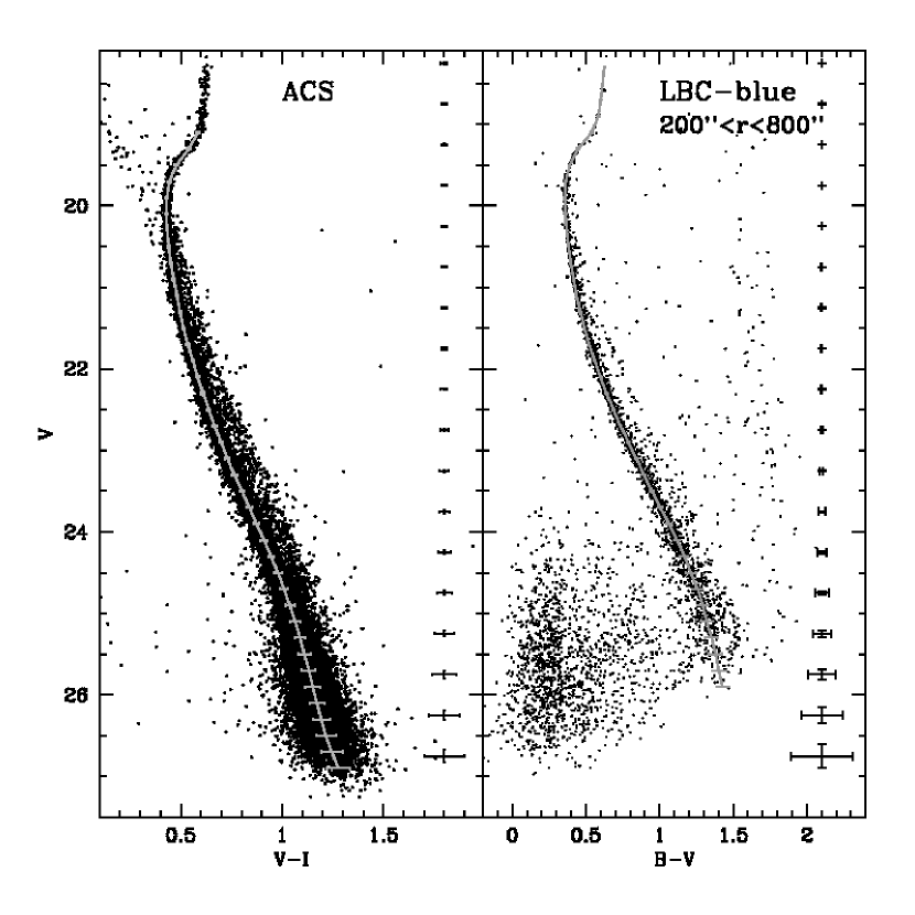
Figure 3.— CMDs of the ACS and the deep LBC samples (left and right panels, respectively). The mean ridge line is shown as a solid line.

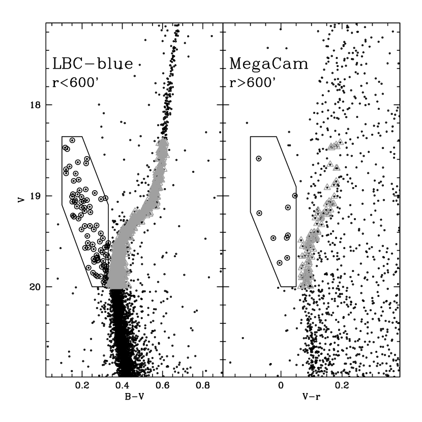
Figure 4.— CMDs showing the selection of the BSS population (open circles) in the shallow LBC and the MEGACAM samples (left and right panels, respectively). The grey open triangles marks the population of sub-giant and RGB stars used as reference in the study of the BSS radial distribution.

Figure 5.— Cumulative radial distribution of BSSs (solid line) and sub-giant+RGB stars (dashed line), as a function of the projected distance from the cluster center.

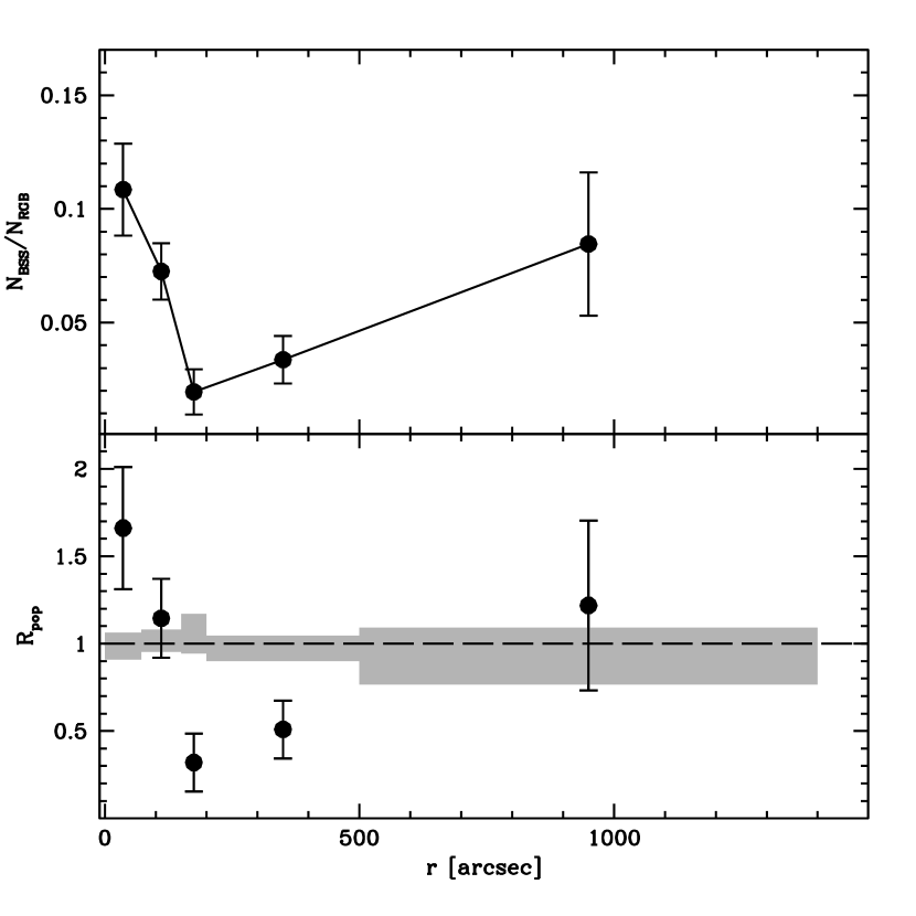
Figure 6.— BSS rardial distribution. Upper panel: number of BSSs with respect to that of reference (SGB+RGB) stars, plotted as a function of the distance from the cluster center. Lower panel double normalized ratio (see text) of BSSs (dots and error bars) and reference stars (gray regions). The distribution is clearly bimodal, with a minimum at $r_{\rm min}\simeq 180\arcsec$.

Figure 7.— Photometric completeness $\phi$ as a function of $V$ for the two data sets. The ACS and deep LBC data-sets have been divided into three and four concentric annuli areas of same completeness, respectively. The solid horizontal line shows the limits of 50% of completeness.

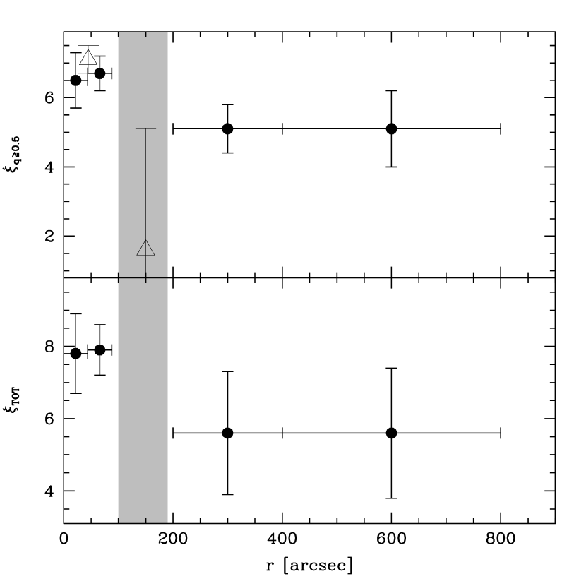
Figure 8.— Minimum and total binary fractions (solid circles in the upper and lower panels, respectively) as a function of radial distance from the cluster center. The grey area show the region excluded from the analysis because of the very low photometric completeness. The empty triangles in the upper panel mark the estimate from Milone et al. (2012).

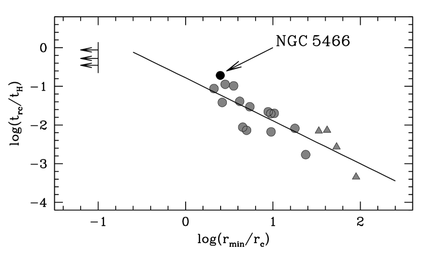
Figure 9.— Core relaxation time ($t_{\rm rc}$) normalized to the age of the Universe ($t_{\rm H}$ = 13.7 Gyr), as a function of $r_{\rm min}/r_{c}$ (with $r_{\rm min}=180\arcsec$ being the position of the minimum of the BSS radial distribution). The figure is the same as Figure 4 in F12: the arrows indicate the location of the dynamically young clusters (Family I); grey circles are GCs of intermediate age (Family II in F12, plus M10 studied by Dalessandro et al., 2013); grey triangles are dynamically old clusters (Family III). The location of NGC 5466 in this plane is marked with the black circle and clearly shows that this is the second youngest member of Family III.

Table 1Log of the observations

Data-set	Number of exposures	Filter	Exposure time	Date of observations
			(s)
Shallow Sample
LBC-blue	1	$B$	5	2007-06-17
	7	$B$	90	2007-06-17
	1	$V$	5	2007-06-17
	7	$V$	60	2007-06-17
MEGACAM	1	$g$	90	2004-04-14
	1	$r$	180	2004-04-14
Deep Sample
LBC-blue	11	$B$	400	2010-04-11
	15	$V$	200	2010-04-11
ACS	5	$V_{606}$	340	2006-04-12
	5	$I_{814}$	350	2006-04-12

Table 2BSS radial distribution in NGC 5466

$r_{i}\arcsec$	$r_{e}\arcsec$	$N_{\rm BSS}$	$N_{\rm RGB}$	Fraction of cluster’s luminosity
0	72	32 (0.01)	295 (0.05)	0.211
72	150	37 (0.02)	510 (0.17)	0.353
150	200	4 (0.02)	204 (0.17)	0.136
200	500	11 (0.27)	321 (2.01)	0.230
500	1400	10 (2.16)	109 (16.36)	0.07

Table 3Binary fraction of NGC 5466

$r_{i}\arcsec$	$r_{e}\arcsec$	$\xi_{min}$	$\xi_{TOT}$
0	44	($6.5\pm 0.8$)%	($7.8\pm 1.1$)%
44	88	($6.7\pm 0.5$)%	($7.9\pm 0.7$)%
200	400	($5.1\pm 0.7$)%	($5.6\pm 1.7$)%
400	800	($5.1\pm 1.1$)%	($5.6\pm 1.8$)%

References

- Bailyn (1992) Bailyn, C. D. 1992, ApJ, 392, 519
- Bailyn (1995) Bailyn, C. D. 1995, ARA&A, 33, 133
- Beccari et al. (2008) Beccari, G., Lanzoni, B., Ferraro, F. R., et al. 2008, ApJ, 679, 712
- Beccari et al. (2011) Beccari, G., Sollima, A., Ferraro, F. R., et al. 2011, ApJ, 737, L3
- Beccari et al. (2012) Beccari, G., Lützgendorf, N., Olczak, C., et al. 2012, ApJ, 754, 108
- Bellazzini et al. (1995) Bellazzini, M., Pasquali, A., Federici, L., Ferraro, F. R., & Pecci, F. F. 1995, ApJ, 439, 687
- Bellazzini et al. (2002) Bellazzini, M., Fusi Pecci, F., Messineo, M., Monaco, L., & Rood, R. T. 2002, AJ, 123, 1509
- Belokurov et al. (2006) Belokurov, V., Evans, N. W., Irwin, M. J., Hewett, P. C., & Wilkinson, M. I. 2006, ApJ, 637, L29
- Bertin & Arnouts (1996) Bertin, E., & Arnouts, S. 1996, A&AS, 117, 393
- Contreras Ramos et al. (2012) Contreras Ramos, R., Ferraro, F. R., Dalessandro, E., Lanzoni, B., & Rood, R. T. 2012, ApJ, 748, 91
- Cote et al. (1996) Cote, P., Pryor, C., McClure, R. D., Fletcher, J. M., & Hesser, J. E. 1996, AJ, 112, 574
- Dalessandro et al. (2008) Dalessandro, E., Lanzoni, B., Ferraro, F. R., et al. 2008, ApJ, 681, 311
- Dalessandro et al. (2009) Dalessandro, E., Beccari, G., Lanzoni, B., et al. 2009, ApJS, 182, 509
- Dalessandro et al. (2011) Dalessandro, E., Lanzoni, B., Beccari, G., et al. 2011, ApJ, 743, 11
- Dalessandro et al. (2013) Dalessandro, E., Ferraro, F. R., Lanzoni, B., et al. 2013, ApJ, 770, 45
- Djorgovski (1993) Djorgovski, S. 1993, in ASPC Conf. Ser. 50, Structure and Dynamics of Globular Clusters, ed. S. G. Djorgovski & G. Meylan (San Francisco: ASP), 373D
- Dotter et al. (2007) Dotter, A., Chaboyer, B., Jevremović, D., et al. 2007, AJ, 134, 376
- Fekadu et al. (2007) Fekadu, N., Sandquist, E. L., & Bolte, M. 2007, ApJ, 663, 277
- Ferraro et al. (1991) Ferraro, F. R., Clementini, G., Fusi Pecci, F., & Buonanno, R. 1991, MNRAS, 252, 357
- Ferraro et al. (1992) Ferraro, F. R., Fusi Pecci, F., & Buonanno, R. 1992, MNRAS, 256, 376
- Ferraro et al. (1995) Ferraro, F. R., Fusi Pecci, F., & Bellazzini, M. 1995, A&A, 294, 80
- Ferraro et al. (1997) Ferraro, F. R., Paltrinieri, B., Fusi Pecci, F., et al. 1997, A&A, 324, 915
- Ferraro et al. (1999) Ferraro, F. R., Messineo, M., Fusi Pecci, F., et al. 1999, AJ, 118, 1738
- Ferraro et al. (2003) Ferraro, F. R., Sills, A., Rood, R. T., Paltrinieri, B., & Buonanno, R. 2003, ApJ, 588, 464
- Ferraro et al. (2004) Ferraro, F. R., Beccari, G., Rood, R. T., et al. 2004, ApJ, 603, 127
- Ferraro et al. (2006a) Ferraro, F. R., Sabbi, E., Gratton, R., et al. 2006a, ApJ, 647, L53
- Ferraro et al. (2006b) Ferraro, F. R., Sollima, A., Rood, R. T., et al. 2006b, ApJ, 638, 433
- Ferraro et al. (2009) Ferraro, F. R., Beccari, G., Dalessandro, E., et al. 2009, Nature, 462, 1028 (F09)
- Ferraro et al. (2012) Ferraro, F. R., Lanzoni, B., Dalessandro, E., et al. 2012, Nature, 492, 393
- Fisher et al. (2005) Fisher, J., Schröder, K.-P., & Smith, R. C. 2005, MNRAS, 361, 495
- Giallongo et al. (2008) Giallongo, E., Ragazzoni, R., Grazian, A., et al. 2008, A&A, 482, 349
- Gilliland et al. (1998) Gilliland, R. L., Bono, G., Edmonds, P. D., et al. 1998, ApJ, 507, 818
- Goldsbury et al. (2010) Goldsbury, R., Richer, H. B., Anderson, J., et al. 2010, AJ, 140, 1830
- Grillmair & Johnson (2006) Grillmair, C. J., & Johnson, R. 2006, ApJ, 639, L17
- Harris (1996) Harris, W. E. 1996, AJ, 112, 1487
- Hill et al. (2006) Hill, J. M., Green, R. F., & Slagle, J. H. 2006, Proc. SPIE, 6267, 62670Y
- Hills & Day (1976) Hills, J. G., & Day, C. A. 1976, Astrophys. Lett., 17, 87
- Hurley & Tout (1998) Hurley, J., & Tout, C. A. 1998, MNRAS, 300, 977
- Hut et al. (1992) Hut, P., McMillan, S., Goodman, J., et al. 1992, PASP, 104, 981
- King (1966) King, I.R. 1966, AJ, 71, 64
- Knigge et al. (2009) Knigge, C., Leigh, N., & Sills, A. 2009, Nature, 457, 288
- Kroupa (2002) Kroupa, P. 2002, Science, 295, 82
- Kryachko et al. (2011) Kryachko, T., Samokhvalov, A., & Satovskiy, B. 2011, Peremennye Zvezdy Prilozhenie, 11, 20
- Lanzoni et al. (2007a) Lanzoni, B., Sanna, N., Ferraro, F. R., et al. 2007a, ApJ, 663, 1040
- Lanzoni et al. (2007b) Lanzoni, B., Dalessandro, E., Ferraro, F. R., et al. 2007b, ApJ, 663, 267
- Leigh et al. (2013) Leigh, N., Knigge, C., Sills, A., et al. 2013, MNRAS, 428, 897
- Mathieu & Geller (2009) Mathieu, R. D., & Geller, A. M. 2009, Nature, 462, 1032
- Mateo et al. (1990) Mateo, M., Harris, H. C., Nemec, J., & Olszewski, E. W. 1990, AJ, 100, 469
- Mateo (1996) Mateo, M. 1996, The Origins, Evolution, and Destinies of Binary Stars in Clusters, ASPCS, 90, 21
- McCrea (1964) McCrea, W. H. 1964, MNRAS, 128, 147
- McMillan (1991) McMillan, S. L. W. 1991, The Formation and Evolution of Star Clusters, 13, 324
- Meylan & Heggie (1997) Meylan, G., & Heggie, D. C. 1997, A&A Rev., 8, 1
- Milone et al. (2012) Milone, A. P., Piotto, G., Bedin, L. R., et al. 2012, A&A, 540, A16
- Miocchi et al. (2013) Miocchi, P., Lanzoni, B., Ferraro, F. R., et al. 2013, arXiv:1307.6035
- Nemec & Harris (1987) Nemec, J. M., & Harris, H. C. 1987, ApJ, 316, 172
- Paresce et al. (1992) Paresce, F., de Marchi, G., & Ferraro, F. R. 1992, Nature, 360, 46
- Pooley & Hut (2006) Pooley, D., & Hut, P. 2006, ApJ, 646, L143
- Ragazzoni et al. (2006) Ragazzoni, R., et al. 2006, Proc. SPIE, 6267, 626710
- Ransom et al. (2005) Ransom, S. M., Hessels, J. W. T., Stairs, I. H., et al. 2005, Science, 307, 892
- Renzini & Buzzoni (1986) Renzini A., Buzzoni A., 1986, ASSL, 122, 195
- Rey et al. (1998) Rey, S.-C., Lee, Y.-W., Byun, Y.-I., & Chun, M.-S. 1998, AJ, 116, 1775
- Robin et al. (2003) Robin, A. C., Reylé, C., Derrière, S., & Picaud, S. 2003, A&A, 409, 523
- Romani & Weinberg (1991) Romani, R. W., & Weinberg, M. D. 1991, ApJ, 372, 487
- Sarajedini et al. (2007) Sarajedini, A., Bedin, L. R., Chaboyer, B., et al. 2007, AJ, 133, 1658
- Shara et al. (1997) Shara, M. M., Saffer, R. A., & Livio, M. 1997, ApJ, 489, L59
- Sirianni et al. (2005) Sirianni, M., et al. 2005, PASP, 117, 1049
- Sollima et al. (2007) Sollima, A., Beccari, G., Ferraro, F. R., Fusi Pecci, F., & Sarajedini, A. 2007, MNRAS, 380, 781
- Sollima et al. (2008) Sollima, A. et al. 2008, A&A, 481, 701
- Sollima et al. (2010) Sollima, A., Carballo-Bello, J. A., Beccari, G., et al. 2010, MNRAS, 401, 577
- Stetson (1987) Stetson, P. B. 1987, PASP, 99, 191
- Stetson (1994) Stetson, P. B. 1994, PASP, 106, 250
- Stetson (2000) Stetson, P. B. 2000, PASP, 112, 925
- Wilson (1975) Wilson, C. P. 1975, AJ, 80, 175
- Zinn & Searle (1976) Zinn, R., & Searle, L. 1976, ApJ, 209, 734