Spectrum Optimization in Multi-User Multi-Carrier Systems with Iterative Convex and Nonconvex Approximation Methods

Abstract

Several practical multi-user multi-carrier communication systems are characterized by a multi-carrier interference channel system model where the interference is treated as noise. For these systems, spectrum optimization is a promising means to mitigate interference. This however corresponds to a challenging nonconvex optimization problem. Existing iterative convex approximation (ICA) methods consist in solving a series of improving convex approximations and are typically implemented in a per-user iterative approach. However they do not take this typical iterative implementation into account in their design. This paper proposes a novel class of iterative approximation methods that focuses explicitly on the per-user iterative implementation, which allows to relax the problem significantly, dropping joint convexity and even convexity requirements for the approximations. A systematic design framework is proposed to construct instances of this novel class, where several new iterative approximation methods are developed with improved per-user convex and nonconvex approximations that are both tighter and simpler to solve (in closed-form). As a result, these novel methods display a much faster convergence speed and require a significantly lower computational cost. Furthermore, a majority of the proposed methods can tackle the issue of getting stuck in bad locally optimal solutions, and hence improve solution quality compared to existing ICA methods.

I Introduction

The delivery of reliable and high-speed communication services to a large set of wireless or wireline end-users has become a true challenge. This is due to the scarcity of the available frequency bandwidth resources, the enormous growth of data traffic with stringent quality-of-service (QoS) requirements, and the increasing number of users. As a result many modern communication systems are forced to follow a setup in which multiple users share a common frequency bandwidth that is reused in time and frequency so as to improve the spectral efficiency. However, in these systems interference among the users impacts the transmission of each user and can result in a significant performance degradation such as decreased data rates and reduced reliability. In fact, interference is identified as one of the major bottlenecks in multi-user transmission [2].

The development and optimization of multi-user interference mitigation techniques is thus an important consideration. These techniques adopt an approach of coordinating the transmission of multiple users taking the impact of interference explicitly into account. In particular, interference mitigation via spectrum optimization is recognized as a very powerful technique. It consists of the joint coordination of the transmit spectrum, i.e., transmit powers over all frequency carriers, of the interfering users so that the spectral efficiency is improved. This can lead to a maximization of the data rates for a given transmit power budget [3], a minimization of the transmit powers for mininum target data rates [4, 5], some fair trade-off between these objectives [6], or even a maximization of the signal to noise ratio (SNR) margin [7, 8]. We want to highlight here that our target system model considers spectrum optimization only, i.e., without any joint signal coordination at the transmitter or the receiver side. From an information-theoretic point of view, our considered system corresponds to a multi-carrier interference channel. Here different users try to communicate their separate information over an interference coupled channel. The capacity region of the interference channel under all regimes is still an open problem. For specific subclasses of the interference channels the capacity regions are obtained [9, 10, 11, 12, 13], or outer regions are derived [14, 15, 16]. For practical systems where the couplings are typically weaker than the direct channel, treating interference as additive white Gaussian noise (AWGN) has been a very important practical communication strategy in operational networks. This is a model that has been widely considered in literature. More specifically, spectrum optimization or power control (for multi-carrier and single-carrier transmission, respectively) has been considered for different systems: power control for code division multiple access (CDMA) in cellular networks [17, 18], power control for cognitive wireless networks [19], power control for femtocell networks [20, 21], general power control [22, 23, 24, 25], spectrum optimization for multi-user multi-channel cellular relay networks [26], spectrum optimization for heterogeneous wireless access networks [27], and cross-layer power and spectrum optimization [28, 29, 30].

In this paper we will focus on the general case of spectrum optimization for multi-user multi-carrier systems where the interference is treated as AWGN. One important example is the digital subscriber line (DSL) system where multiple users transmit over twisted pair copper lines that are bundled in large cable binders. Each user adopts discrete multitone (DMT) modulation, a multicarrier transmission technique where the frequency band is divided into independent subcarriers, also referred to as tones. At the high frequencies used by DSL DMT technology, electromagnetic coupling among the different twisted pair copper lines occurs within the same cable binder, which is also referred to as crosstalk interference or just crosstalk. Tackling this type of interference using spectrum optimization is also referred to as dynamic spectrum management (DSM) level-2, spectrum balancing or spectrum coordination in the DSL literature. Note that although we will follow this line of spectrum optimization theory developed for DSL wireline communications, the spectrum optimization methods developed in this paper are similarly applicable for general interference-limited multi-user systems that follow an interference channel system model.

Many spectrum optimization methods have been proposed in the literature to solve the corresponding spectrum optimization problem. These methods range from fully autonomous [31, 32, 33], and distributed [32, 34, 35, 36, 37], to centralized methods [38, 39, 40, 41, 42, 43]. In particular, the approach of iterative convex approximation (ICA) has been recognized to be very efficient, as exemplified by the CA-DSB [32, 44] and SCALE [35] algorithms. These algorithms consist in solving a series of improving convex approximations to the original nonconvex problem, until convergence to a locally optimal solution or a stationary point. They are furthermore characterized by a low computational cost, high speed of convergence, and potential distributed and asynchronous implementations. The complexity of this ICA approach depends on two factors: (i) the type of approximation, where a tighter approximation generally results in fewer iterations until convergence, and (ii) the computational cost of solving the corresponding approximation. Such ICA algorithms (for distributed or centralized computation) are typically implemented in a per-user iterative approach, as this is demonstrated to be highly efficient [33, 32, 45, 34, 35, 36] for practical and implementational reasons and it results in good performance. For instance, it is shown in [32] that these iterative implementations can solve small- to medium-scale DSL scenarios, i.e., up to 6 users and 1000 tones, within a few seconds. However, for large-scale DSL scenarios, i.e. 10 to 50 users and 4000 tones, these iterative methods can take several minutes or even hours. Moreover, it is shown in [32] that these methods can sometimes get stuck in bad locally optimal solutions.

In this paper we design a novel class of iterative approximation methods that explicitly focus on the typical per-user iterative implementation. It will be shown that in this setting, joint convexity and even convexity requirements on the approximations can be relaxed, resulting in a much larger degree of freedom to design convergent iterative algorithms. A design framework will be proposed that provides a design strategy for developing improved (convex as well as nonconvex) approximations that are much tighter and simpler to solve (i.e., in closed-form) than those of existing state-of-the-art ICA methods. With this design framework, ten novel methods are developed that are provably better than existing ICA methods in terms of faster convergence and lower computational cost. Furthermore, it will be shown how some of the proposed methods can tackle the issue of getting stuck in bad locally optimal solutions, and can thus even improve the final solution quality (i.e., improve data rate performance). Moreover, the flexibility of the proposed novel class allows the combination of different types of approximations over different tones and users, which even further improves the trade-off between computational cost and solution quality. Both a reduction in the number of iterations required for convergence and an improvement in solution quality will be demonstrated using a realistic DSL simulator.

This text is organized as follows. Section II briefly describes the multi-user multi-carrier system model and spectrum optimization. In Section III, existing ICA spectrum optimization approaches are explained and the typical per-user iterative implementation is highlighted. A general outline for our novel class of algorithms is described in Section IV-A, and the corresponding design framework is constructed in Section IV-B. Using this framework, ten novel methods are constructed in Section IV-C, which are analyzed and generalized in Section IV-D. Potential iterative fixed point update implementations are considered and discussed in Section IV-E. Improved solution quality of the proposed methods based on nonconvex approximations is discussed in Section IV-F, and frequency and user selective allocation of approximations is discussed in Section IV-G. Finally, Section V provides extensive simulation results for different realistic ADSL/ADSL2/VDSL scenarios and highlights the improved performance of the proposed novel class of algorithms with respect to that of state-of-the-art ICA methods in terms of convergence speed, computational cost and solution quality.

II System Model and Spectrum Optimization

We consider a multi-user multi-carrier system with a set $\mathcal{N}=\{1,\ldots,N\}$ of $N$ users and a set $\mathcal{K}=\{1,\ldots,K\}$ of $K$ tones (i.e., frequency carriers). We consider synchronous transmission without intercarrier interference. As we focus on spectrum optimization, we assume no signal coordination at the transmitters or at the receivers. Furthermore, we make the practical assumption that interference is treated as AWGN, which is for instance a standard valid assumption in DSL communications when the number of interferers is large [46]. Under these typical assumptions for spectrum coordination [3], the spectrum optimization problem (SO problem) can be formulated as follows

$$\begin{array}[]{lcl}\mathrm{(SO~{}problem):}&{\displaystyle\min_{\mathbf{s}_{k}\in\mathcal{S}_{k},k\in\mathcal{K}}}&{\displaystyle\sum_{k\in\mathcal{K}}f_{k}(\mathbf{s}_{k})}\\ &\mathrm{subject~{}to}&{\displaystyle\sum_{k\in\mathcal{K}}\mathbf{s}_{k}\leq\mathbf{P}^{\mathrm{tot}}},\end{array}$$ (1)

with $\mathbf{s}_{k}=[s_{k}^{1},\ldots,s_{k}^{N}]^{T}$ denoting transmit powers of all users on tone $k$, the vector constant $\mathbf{P}^{\mathrm{tot}}=[P^{1,\mathrm{tot}},\ldots,P^{N,\mathrm{tot}}]^{T}$ denoting total power budgets for all users, and the set $\mathcal{S}_{k}=\{s_{k}^{n},n\in\mathcal{N}\mid 0\leq s_{k}^{n}\leq s_{k}^{n,\mathrm{mask}},\forall n\in\mathcal{N}\}$ denoting the feasible set on each tone $k$ with a maximum spectral transmit constraint $s_{k}^{n,\mathrm{mask}}$ for user $n$. We also define the set $\mathcal{S}_{k}^{n}=\{s_{k}^{n}\mid 0\leq s_{k}^{n}\leq s_{k}^{n,\mathrm{mask}}\}$ which will be used later in the text.

Each term $f_{k}(\mathbf{s}_{k})$ in the objective function corresponds to the following nonconvex function

$$f_{k}(\mathbf{s}_{k})=-\sum_{n\in\mathcal{N}}w_{n}\log\left(1+\frac{s_{k}^{n}}{{\displaystyle\sum_{m\neq n}}a_{k}^{n,m}s_{k}^{m}+z_{k}^{n}}\right),$$ (2)

with $w_{n}$ denoting the weight given to the achievable data rate of user $n$, $a_{k}^{n,m}$ denoting the normalized channel gains from transmitter $m$ to receiver $n$ on tone $k$, and $z_{k}^{n}$ denoting the normalized AWGN power for line $n$ on tone $k$. The SNR gap [47] is also included in the normalized channel gains and noise power. The optimization problem (1) with objective function (2) corresponds to a standard weighted sum of achievable data rates maximization over multiple carriers and under a separate power constraint for each user.

We also define symbols $\mathrm{int}_{k}^{n}$ for the interference (plus noise) of user $n$ on tone $k$, and $\mathrm{rec}_{k}^{n}$ for the received signal of user $n$ on tone $k$, so as to facilitate notation in the remainder of the text:

$$\mathrm{int}_{k}^{n}={\displaystyle\sum_{m\neq n}a_{k}^{n,m}s_{k}^{m}+z_{k}^{n}},$$ (3)

$$\mathrm{rec}_{k}^{n}={\displaystyle s_{k}^{n}+\sum_{m\neq n}a_{k}^{n,m}s_{k}^{m}+z_{k}^{n}=s_{k}^{n}+\mathrm{int}_{k}^{n}},$$ (4)

so that $f_{k}(\mathbf{s}_{k})$ can be written as

$$f_{k}(\mathbf{s}_{k})=-\sum_{n\in\mathcal{N}}w_{n}\log\left(1+\frac{s_{k}^{n}}{\mathrm{int}_{k}^{n}}\right)=-\sum_{n\in\mathcal{N}}w_{n}\log\left(\frac{\mathrm{rec}_{k}^{n}}{\mathrm{int}_{k}^{n}}\right).$$

With the above definitions, we can also define the achievable data rates and bit loadings as

$$R^{n}=\sum_{k\in\mathcal{K}}b_{k}^{n}=\sum_{k\in\mathcal{K}}\log\left(1+\frac{s_{k}^{n}}{\mathrm{int}_{k}^{n}}\right),$$ (5)

where $R^{n}$ and $b_{k}^{n}$ are the achievable data rate of user $n$ and the achievable bit loading of user $n$ on tone $k$, respectively.

III Spectrum Optimization Through Iterative Convex Approximation

The ICA approach to tackle the SO problem consists in solving a series of improving convex approximations. This procedure is given in Algorithm 1. In line 1 an initial approximation point $\mathbf{\tilde{s}}_{k},k\in\mathcal{K},$ is chosen from the set $\{\mathbf{s}_{k}\in\mathcal{S}_{k},k\in\mathcal{K}\}$. This initial point can be chosen based on a high SNR heuristic [35], a zero transmit power value [32], or even randomly [29, 30]. In line 3 the nonconvex function $f_{k}(\mathbf{s}_{k})$ is approximated by a convex function $f_{k}^{\mathrm{cvx}}(\mathbf{s}_{k};\mathbf{\tilde{s}}_{k})$ built around the chosen approximation point $\mathbf{\tilde{s}}_{k}$. We want to highlight that the convex approximation depends on the chosen approximation point $\mathbf{\tilde{s}}_{k}$. The resulting convex problem is then solved in line 4 to obtain an improved solution, which is used as a new approximation point in line 5. This is iterated in a loop (lines 2-6) until convergence to a stationary point.

Algorithm 1 Iterative convex approximation (ICA) for SO problem (1)

1:  Choose an initial approximation point $\mathbf{\tilde{s}}_{k}\in\mathcal{S}_{k},k\in\mathcal{K}$

2:  while not converged to stationary point do

3:     Approximate $f_{k}(\mathbf{s}_{k})$ in problem (1) by convex function $f_{k}^{\mathrm{cvx}}(\mathbf{s}_{k};\mathbf{\tilde{s}}_{k}),k\in\mathcal{K}$

4:     Solve corresponding convex problem to obtain $\mathbf{s}_{k}^{\mathrm{cvx},*},k\in\mathcal{K}$

5:     Set $\mathbf{\tilde{s}}_{k}=\mathbf{s}_{k}^{\mathrm{cvx},*},\forall k\in\mathcal{K}$

6:  end while

The ICA procedure is guaranteed to converge to a locally optimal solution or a stationary point of the SO problem under the following conditions [48]:

$$f_{k}^{\mathrm{cvx}}(\mathbf{\tilde{s}}_{k};\mathbf{\tilde{s}}_{k})=f_{k}(\mathbf{\tilde{s}}_{k}),\forall k\in\mathcal{K},$$ (6)

$$\nabla f_{k}^{\mathrm{cvx}}(\mathbf{\tilde{s}}_{k};\mathbf{\tilde{s}}_{k})=\nabla f_{k}(\mathbf{\tilde{s}}_{k}),\forall k\in\mathcal{K},$$ (7)

$$f_{k}^{\mathrm{cvx}}(\mathbf{s}_{k};\mathbf{\tilde{s}}_{k})\geq f_{k}(\mathbf{{s}}_{k}),\forall\mathbf{s}_{k}\in\mathcal{S}_{k},k\in\mathcal{K},$$ (8)

which impose that

• the approximation $f_{k}^{\mathrm{cvx}}(\mathbf{s}_{k};\mathbf{\tilde{s}}_{k})$ coincides at first-order with the true objective function $f_{k}(\mathbf{{s}}_{k})$ around the approximation point $\mathbf{\tilde{s}}_{k},k\in\mathcal{K}$, with equations (6)–(7),

• the approximation is an upper bound on the true objective function on the whole feasible set $\mathcal{S}_{k}$, via inequality (8).

The CA-DSB and SCALE algorithms are two effective ICA procedures that use the following convex approximations:

$$f_{k}^{\mathrm{CADSB}}(\mathbf{s}_{k},\mathbf{\tilde{s}}_{k})=-\sum_{n\in\mathcal{N}}\left[w_{n}\log\left(\mathrm{rec}_{k}^{n}\right)\right]+\sum_{n\in\mathcal{N}}b_{k}^{n}(\mathbf{\tilde{s}}_{k})s_{k}^{n}+c_{k}^{n}(\mathbf{\tilde{s}}_{k})$$ (9)

$$f_{k}^{\mathrm{SCALE}}(\mathbf{s}_{k},\mathbf{\tilde{s}}_{k})=-\sum_{n\in\mathcal{N}}\left[w_{n}\alpha_{k}^{n}(\mathbf{\tilde{s}}_{k}^{n})\log\left(\frac{s_{k}^{n}}{\mathrm{int}_{k}^{n}}\right)\right]+c_{k}^{n}(\mathbf{\tilde{s}}_{k})$$ (10)

in which parameters $b_{k}^{n}(\mathbf{\tilde{s}}_{k})$, $\alpha_{k}^{n}(\mathbf{\tilde{s}_{k}})$ and $c_{k}^{n}(\mathbf{\tilde{s}}_{k})$ are constants that depend on the approximation point $\mathbf{\tilde{s}}_{k}$, and which are computed in closed-form such that conditions (6)-(8) are satisfied, see [32, 35]. For instance, the following closed-form expressions hold for $b_{k}^{n}(\mathbf{\tilde{s}}_{k})$ and $\alpha_{k}^{n}(\mathbf{\tilde{s}}_{k})$:

$$b_{k}^{n}(\tilde{\mathbf{s}}_{k})=\sum_{m\neq n}\frac{w_{m}a_{k}^{m,n}}{{\displaystyle\mathrm{int}_{k}^{m}|_{\mathbf{s}_{k}^{-m}=\mathbf{\tilde{s}}_{k}^{-m}}}},$$ (11)

$$\alpha_{k}^{n}(\mathbf{\tilde{s}}_{k})=\frac{\tilde{s}_{k}^{n}}{\mathrm{rec}_{k}^{n}|_{\mathbf{s}_{k}=\mathbf{\tilde{s}}_{k}}}.$$ (12)

where $\mathrm{expression(\mathbf{x})}|_{\mathbf{x}=\mathbf{x}_{0}}$ means that the value of the variable $\mathbf{x}$ in the expression is fixed at $\mathbf{x}=\mathbf{x}_{0}$, and where $\mathbf{s}_{k}^{-n}$ refers to the vector containing transmit powers on tone $k$ of all users except for user $n$. As such, it can be seen that constructing the convex approximations, i.e., line 3 of Algorithm 1, is very simple, whereas line 4 corresponds to solving the convex problem and constitutes the main part of the computational cost.

For the concrete implementation of ICA, one typically follows a per-user iterative approach, where each user iteratively computes its own transmit powers taking the fixed interference of the other users into account. This is done for several reasons: (i) it allows for distributed implementations, (ii) it allows the use of simple bisection searches to solve the per-user dual problem (as will be discussed later in this section), (iii) it allows to take the bound constraints into account with a simple projection operation, (iv) it doesn’t require any stepsize tuning, and (v) most importantly, it has been demonstrated in the literature [45, 32] to have fast convergence and good performance for small- to medium-scale practical DSL scenarios. Because of these practically interesting and implementationally efficient reasons, the per-user iterative implementation has been the preferred scheme for spectrum optimization (in centralized [32, 45] as well as distributed implementations [31, 32, 34, 35, 36]). The typical per-user iterative implementation is shown in Algorithm 2,

Algorithm 2 Per-user iterative ICA approach

1:  Choose an initial approximation point $\mathbf{\tilde{s}}_{k}\in\mathcal{S}_{k},k\in\mathcal{K}$

2:  for outer iterations do

3:   for  user $n=1$ to $N$ do

4:    for inner iterations do

5:      Update per-user convex approximation $f_{k}^{\mathrm{cvx}}(s_{k}^{n};\mathbf{\tilde{s}}_{k}^{-n},\mathbf{\tilde{s}}_{k})$ in $\tilde{s}_{k}^{n},k\in\mathcal{K}$ to obtain (14)

6:      Solve per-user convex problem (14) to obtain $s_{k}^{\mathrm{cvx},n,*},k\in\mathcal{K}$

7:      Set $\tilde{s}_{k}^{n}=s_{k}^{\mathrm{cvx},n,*},k\in\mathcal{K}$

8:    end for

9:   end for

10:  end for

where line 2 corresponds to a fixed number of outer iterations over all users (one can also use instead the stopping criterion used in line 2 of Algorithm 1), line 3 is the iteration over the users, and lines 4 to 8 focus on solving the following per-user version of the SO problem for a given user $n$:

$$\begin{array}[]{cl}{\displaystyle\min_{s^{n}_{k}\in\mathcal{S}_{k}^{n},k\in\mathcal{K}}}&{\displaystyle\sum_{k\in\mathcal{K}}f_{k}(s^{n}_{k};\mathbf{\tilde{s}}_{k}^{-n})}\\ \mathrm{subject~{}to}&{\displaystyle\sum_{k\in\mathcal{K}}s^{n}_{k}\leq\mathbf{P}^{n,\mathrm{tot}}}.\end{array}$$ (13)

More specifically, lines 4 to 8 come down to solving (13) with an iterative approximation approach, performing a series of inner iterations where each approximation (line 6 of Algorithm 2) corresponds to the following per-user problem

$$\begin{array}[]{cl}{\displaystyle\min_{s^{n}_{k}\in\mathcal{S}_{k}^{n},k\in\mathcal{K}}}&{\displaystyle\sum_{k\in\mathcal{K}}f_{k}^{\mathrm{cvx}}(s^{n}_{k};\mathbf{\tilde{s}}_{k}^{-n},\mathbf{\tilde{s}}_{k})}\\ \mathrm{subject~{}to}&{\displaystyle\sum_{k\in\mathcal{K}}s^{n}_{k}\leq\mathbf{P}^{n,\mathrm{tot}}}.\end{array}$$ (14)

We want to highlight here that the functions $f_{k}(s_{k}^{n};\mathbf{s}_{k}^{-n})$ and $f_{k}^{\mathrm{cvx}}(s_{k}^{n};\mathbf{s}_{k}^{-n},\mathbf{\tilde{s}}_{k})$ are univariate (or one-dimensional) functions in $s_{k}^{n}$, because $\mathbf{s}_{k}^{-n}$ is fixed during the inner iterations of user $n$. The above convex approximated per-user problem (14) is then typically solved by focusing on the following dual problem formulation [32, 35], as this allows easier handling of the constraints:

$${\displaystyle\max_{\lambda_{n}\geq 0}}~{}~{}g(\lambda_{n})$$ (15)

$$\mathrm{~{}~{}~{}~{}with~{}~{}}{\displaystyle g(\lambda_{n}):=-\lambda_{n}P^{n,\mathrm{tot}}+\sum_{k\in\mathcal{K}}\underbrace{\left[\min_{s_{k}^{n}\in\mathcal{S}_{k}^{n}}f_{k}^{\mathrm{cvx}}(s_{k}^{n};\mathbf{\tilde{s}}_{k}^{-n},\mathbf{\tilde{s}}_{k})+\lambda_{n}s_{k}^{n}\right]}_{(\mathrm{SUB})}}.$$ (16)

The dual problem (15) is a univariate problem in the dual variable $\lambda_{n}$, which can be solved using a simple bisection search, or (sub-)gradient update approaches [39]. However, the evaluation of the objective function $g(\lambda_{n})$ corresponds to an optimization problem on its own, i.e., (16). This problem can be decomposed over tones for a given $\lambda_{n}$, resulting in $K$ independent univariate subproblems, i.e., SUB in (16), which are convex subproblems as $f_{k}^{\mathrm{cvx}}(s_{k}^{n};\mathbf{\tilde{s}}_{k}^{-n},\mathbf{\tilde{s}}_{k})$ is convex in $s_{k}^{n}$. This is also referred to as dual decomposition. For both CA-DSB, i.e., $f_{k}^{\mathrm{cvx}}(s_{k}^{n};\mathbf{\tilde{s}}_{k}^{-n},\mathbf{\tilde{s}}_{k})=f_{k}^{\mathrm{CADSB}}(s_{k}^{n};\mathbf{\tilde{s}}_{k}^{-n},\mathbf{\tilde{s}}_{k})$, and SCALE, i.e., $f_{k}^{\mathrm{cvx}}(s_{k}^{n};\mathbf{\tilde{s}}_{k}^{-n},\mathbf{\tilde{s}}_{k})=f_{k}^{\mathrm{SCALE}}(s_{k}^{n};\mathbf{\tilde{s}}_{k}^{-n},\mathbf{\tilde{s}}_{k})$, it can be shown that each independent decomposed subproblem in (16) can be solved by computing the roots of a polynomial of degree $N$, which can only be done in closed-form when $N\leq 4$, i.e., with 4 users or less. Therefore iterative fixed point updates were proposed in [32, 35] to solve the subproblems in (16), instead of computing closed-form solutions.

TABLE I: Decomposition of 1D function for different methods, and max degree of corresponding polynomial to solve subproblems in (22). Second naming scheme is described in Section IV-D. C and NC stand for convex and nonconvex.

Methods	$f_{k}^{1}(s_{k}^{n};\mathbf{s}_{k}^{-n},\mathbf{\tilde{s}}_{k},\theta)$	$f_{k}^{2}(s_{k}^{n};\mathbf{s}_{k}^{-n},\mathbf{\tilde{s}}_{k},\theta)$	Degree
ORIG	$-w_{n}\log\left(1+\frac{s_{k}^{n}}{{\displaystyle\mathrm{int}_{k}^{n}}}\right)$	/	$2N-1$
	$\qquad\displaystyle{-\sum_{m\in\mathcal{N}\backslash n}}\left[w_{m}\log\left(1+\frac{s_{k}^{m}}{\mathrm{int}_{k}^{m}}\right)\right]$
CADSB	$\displaystyle{-w_{n}\log\left(s_{k}^{n}+\mathrm{int}_{k}^{n}\right)}$	$\displaystyle{+\sum_{n\in\mathcal{N}}}\left[w_{n}\log\left(\mathrm{int}_{k}^{n}\right)\right]$	$N$
	$\qquad\displaystyle{-\sum_{m\in\mathcal{N}\backslash n}}\left[w_{m}\log\left(s_{k}^{m}+\mathrm{int}_{k}^{m}\right)\right]$
SCALE	$-w_{n}\alpha_{k}^{n}(\mathbf{\tilde{s}}_{k})\log\left(\frac{s_{k}^{n}}{\mathrm{int}_{k}^{n}}\right)-c_{k}^{n}(\mathbf{\tilde{s}}_{k})$	$\displaystyle{\sum_{n\in\mathcal{N}}}\left[w_{n}\alpha_{k}^{n}(\mathbf{\tilde{s}}_{k})\log\left(\frac{s_{k}^{n}}{\mathrm{int}_{k}^{n}}\right)\right]+c_{k}^{n}(\mathbf{\tilde{s}}_{k})$	$N$
	$\displaystyle{-\sum_{m\in\mathcal{N}\backslash n}}\left[w_{m}\alpha_{k}^{m}(\mathbf{\tilde{s}}_{k})\log\left(\frac{s_{k}^{m}}{\mathrm{int}_{k}^{m}}\right)\right]$	$\displaystyle{-\sum_{n\in\mathcal{N}}}\left[w_{n}\log\left(1+\frac{s_{k}^{n}}{\mathrm{int}_{k}^{n}}\right)\right]$
$\begin{matrix}\text{IASB1}\\ \text{(IA1, C)}\end{matrix}$	$-w_{n}\log\left(1+\frac{s_{k}^{n}}{{\displaystyle\mathrm{int}_{k}^{n}}}\right)$	$\displaystyle{-\sum_{m\in\mathcal{N}\backslash n}}\left[w_{m}\log\left(1+\frac{s_{k}^{m}}{\mathrm{int}_{k}^{m}}\right)\right]$	$1$
$\begin{matrix}\text{IASB2}\\ \text{(IA2-$L$, C/NC)}\end{matrix}$	$-w_{n}\log\left(1+\frac{s_{k}^{n}}{{\displaystyle\mathrm{int}_{k}^{n}}}\right)-L_{k}^{n}(s_{k}^{n}-\tilde{s}_{k}^{n})^{2}$	$\displaystyle{-\sum_{m\in\mathcal{N}\backslash n}}\left[w_{m}\log\left(1+\frac{s_{k}^{m}}{\mathrm{int}_{k}^{m}}\right)\right]+L_{k}^{n}(s_{k}^{n}-\tilde{s}_{k}^{n})^{2}$	$2$
$\begin{matrix}\text{IASB3}\\ \text{(IA3-$r$, NC)}\end{matrix}$	$\displaystyle{-w_{n}\log\left(1+\frac{s_{k}^{n}}{\mathrm{int}_{k}^{n}}\right)-w_{q}\log\left(1+\frac{s_{k}^{q}}{\mathrm{int}_{k}^{q}}\right)}$	$\displaystyle{-\sum_{p\in\mathcal{N}\backslash\{n,q\}}}\left[w_{p}\log\left(1+\frac{s_{k}^{p}}{\mathrm{int}_{k}^{p}}\right)\right]$	$3$
$\begin{matrix}\text{IASB4}\\ \text{(IA2-$\alpha$, NC)}\end{matrix}$	$-w_{n}\log\left(1+\frac{s_{k}^{n}}{\mathrm{int}_{k}^{n}}\right)$	$+w_{q}\alpha_{k}^{q}(\mathbf{\tilde{s}}_{k})\log\left(\frac{s_{k}^{q}}{\mathrm{int}_{k}^{q}}\right)+c_{k}^{n}(\mathbf{\tilde{s}}_{k})$	$2$
	$-w_{q}\alpha_{k}^{q}(\mathbf{\tilde{s}}_{k})\log\left(\frac{s_{k}^{q}}{\mathrm{int}_{k}^{q}}\right)-c_{k}^{n}(\mathbf{\tilde{s}}_{k})$	$\displaystyle{-\sum_{m\in\mathcal{N}\backslash n}}\left[w_{m}\log\left(1+\frac{s_{k}^{m}}{\mathrm{int}_{k}^{m}}\right)\right]$
$\begin{matrix}\text{IASB5}\\ \text{(IA3-$\alpha^{2}$, NC)}\end{matrix}$	$-w_{n}\log\left(1+\frac{s_{k}^{n}}{\mathrm{int}_{k}^{n}}\right)$	${\displaystyle\sum_{p\in\{q,t\}}}\left[w_{p}\alpha_{k}^{p}(\mathbf{\tilde{s}}_{k})\log\left(\frac{s_{k}^{p}}{\mathrm{int}_{k}^{p}}\right)\right]+c_{k}^{n}(\mathbf{\tilde{s}}_{k})$	$3$
	$-{\displaystyle\sum_{p\in\{q,t\}}}\left[w_{p}\alpha_{k}^{p}(\mathbf{\tilde{s}}_{k})\log\left(\frac{s_{k}^{p}}{\mathrm{int}_{k}^{p}}\right)\right]-c_{k}^{n}(\mathbf{\tilde{s}}_{k})$	$\displaystyle{-\sum_{m\in\mathcal{N}\backslash n}}\left[w_{m}\log\left(1+\frac{s_{k}^{m}}{\mathrm{int}_{k}^{m}}\right)\right]$
$\begin{matrix}\text{IASB6}\\ \text{(IA1-$\beta$, C)}\end{matrix}$	$-w_{n}(1-\beta_{k}^{n})\log\left(1+\frac{s_{k}^{n}}{{\displaystyle\mathrm{int}_{k}^{n}}}\right)$	$-\beta_{k}^{n}w_{n}\log\left(1+\frac{s_{k}^{n}}{{\displaystyle\mathrm{int}_{k}^{n}}}\right)\displaystyle{-\sum_{m\in\mathcal{N}\backslash n}}\left[w_{m}\log\left(1+\frac{s_{k}^{m}}{\mathrm{int}_{k}^{m}}\right)\right]$	$1$
$\begin{matrix}\text{IASB7}\\ \text{(IA3-$\beta$r, NC)}\end{matrix}$	$-w_{n}(1-\beta_{k}^{n})\log\left(1+\frac{s_{k}^{n}}{\mathrm{int}_{k}^{n}}\right)-w_{q}\log\left(1+\frac{s_{k}^{q}}{\mathrm{int}_{k}^{q}}\right)$	$-\beta_{k}^{n}w_{n}\log\left(1+\frac{s_{k}^{n}}{{\displaystyle\mathrm{int}_{k}^{n}}}\right)\displaystyle{-\sum_{p\in\mathcal{N}\backslash\{n,q\}}}\left[w_{p}\log\left(1+\frac{s_{k}^{p}}{\mathrm{int}_{k}^{p}}\right)\right]$	$3$
$\begin{matrix}\text{IASB8}\\ \text{(IA3-$\beta\alpha^{2}$, NC)}\end{matrix}$	$-w_{n}(1-\beta_{k}^{n})\log\left(1+\frac{s_{k}^{n}}{\mathrm{int}_{k}^{n}}\right)$	$-\beta_{k}^{n}w_{n}\log\left(1+\frac{s_{k}^{n}}{{\displaystyle\mathrm{int}_{k}^{n}}}\right)\displaystyle{-\sum_{m\in\mathcal{N}\backslash n}}\left[w_{m}\log\left(1+\frac{s_{k}^{m}}{\mathrm{int}_{k}^{m}}\right)\right]$	$3$
	$-{\displaystyle\sum_{p\in\{q,t\}}}\left[w_{p}\alpha_{k}^{p}(\mathbf{\tilde{s}}_{k})\log\left(\frac{s_{k}^{p}}{\mathrm{int}_{k}^{p}}\right)\right]-c_{k}^{n}(\mathbf{\tilde{s}}_{k})$	$+{\displaystyle\sum_{p\in\{q,t\}}}\left[w_{p}\alpha_{k}^{p}(\mathbf{\tilde{s}}_{k})\log\left(\frac{s_{k}^{p}}{\mathrm{int}_{k}^{p}}\right)\right]+c_{k}^{n}(\mathbf{\tilde{s}}_{k})$
$\begin{matrix}\text{IASB9}\\ \text{(IA3-$\alpha$L, NC)}\end{matrix}$	$-w_{n}\log\left(1+\frac{s_{k}^{n}}{\mathrm{int}_{k}^{n}}\right)-L_{k}^{n}(s_{k}^{n}-\tilde{s}_{k}^{n})^{2}$	$+w_{q}\alpha_{k}^{q}(\mathbf{\tilde{s}}_{k})\log\left(\frac{s_{k}^{q}}{\mathrm{int}_{k}^{q}}\right)+c_{k}^{n}(\mathbf{\tilde{s}}_{k})+L_{k}^{n}(s_{k}^{n}-\tilde{s}_{k}^{n})^{2}$	$3$
	$-w_{q}\alpha_{k}^{q}(\mathbf{\tilde{s}}_{k})\log\left(\frac{s_{k}^{q}}{\mathrm{int}_{k}^{q}}\right)-c_{k}^{n}(\mathbf{\tilde{s}}_{k})$	$\displaystyle{-\sum_{m\in\mathcal{N}\backslash n}}\left[w_{m}\log\left(1+\frac{s_{k}^{m}}{\mathrm{int}_{k}^{m}}\right)\right]$
$\begin{matrix}\text{IASB10}\\ \text{(IA$N$-$\alpha^{N-1}$, NC)}\end{matrix}$	$-w_{n}\log(1+\frac{s_{k}^{n}}{\mathrm{int}_{k}^{n}})$	$\displaystyle{\sum_{m\in\mathcal{N}\backslash n}}\left[w_{m}\alpha_{k}^{m}(\mathbf{\tilde{s}}_{k})\log\left(\frac{s_{k}^{m}}{\mathrm{int}_{k}^{m}}\right)\right]+c_{k}^{m}(\mathbf{\tilde{s}}_{k})$	$N$
	$\displaystyle{-\sum_{m\in\mathcal{N}\backslash n}}\left[w_{m}\alpha_{k}^{m}(\mathbf{\tilde{s}}_{k})\log\left(\frac{s_{k}^{m}}{\mathrm{int}_{k}^{m}}\right)\right]-c_{k}^{m}(\mathbf{\tilde{s}}_{k})$	$\displaystyle{-\sum_{m\in\mathcal{N}\backslash n}}\left[w_{m}\log\left(1+\frac{s_{k}^{m}}{\mathrm{int}_{k}^{m}}\right)\right]$

The above per-user iterative approach using dual decomposition is recognized as being very effective in tackling the SO problem in the sense that it can find locally optimal solutions to the SO problem with only small computational cost. More specifically, it is shown in [32] that the SO problem up to dimension $KN=2000$ can be solved within a few seconds.

However, there are also some drawbacks when using existing ICA methods (CA-DSB and SCALE). First, the SO problem can have many locally optimal solutions, depending on the considered scenario, where many of those locally optimal solutions can correspond to a quite suboptimal data rate performance, as demonstrated in [32]. Existing ICA methods feature no mechanism to tackle this issue and, depending on the chosen initial point and the considered scenario, may converge to a locally optimal solution with very seriously deteriorated data rate performance. A second issue is that for large-scale scenarios, e.g., DSL scenarios with 10-100 users and more than 1000 tones, ICA methods may take several minutes or even hours. Any improvement to reduce the execution time is desirable for such large-scale scenarios.

IV A Novel Class of Iterative Approximation Methods

Although existing ICA methods are typically implemented in a per-user iterative fashion as shown in the previous section, their design does not take this iterative implementation into account. We propose a novel class of algorithms whose design is tailored to this per-user iterative implementation. We will show that this approach allows to relax the per-user problem to be solved at each iteration, resulting in a much larger design space and can lead to significantly improved convergent iterative spectrum optimization algorithms.

IV-A General Algorithm for Novel Class

When analyzing the typical iterative implementation of Algorithm 2, it can be observed that lines 5 and 6 approximate and solve the per-user problem (14) and thus, following a typical dual decomposition approach, line 6 resorts to solving (possibly in parallel) $K$ independent univariate approximations in the variable $s_{k}^{n}$, one for each tone $k$, as in (16). The univariate approximations can be considered as per-user per-tone approximations.

Existing ICA methods rely on approximations $f_{k}^{\mathrm{cvx}}(\mathbf{s}_{k},\mathbf{\tilde{s}}_{k})$ that are jointly convex in $\mathbf{s}_{k}$. While this joint convexity property guarantees that each per-user problem (13) is convex, it is not a necessary condition (i.e., there are situations where per-user problems are convex while $f_{k}^{\mathrm{cvx}}(\mathbf{s}_{k},\mathbf{\tilde{s}}_{k})$ is not jointly convex). Moreover, although convexity of the per-user problems typically ensures that they can be efficiently minimized, it is not a strict requirement as some nonconvex problems still admit fast resolution techniques. Therefore we propose to relax this joint convexity restriction on $f_{k}^{\mathrm{cvx}}(\mathbf{s}_{k},\mathbf{\tilde{s}}_{k})$ and even drop the requirement of being univariately convex in $s_{k}^{n}$. This results in the novel class of per-user iterative methods of Algorithm 3, where the main difference is that they rely on a univariate approximating function $f_{k}^{\mathrm{app}}(s_{k}^{n};\mathbf{\tilde{s}}_{k}^{-n},\mathbf{\tilde{s}}_{k},\theta)$ that is not necessarily jointly convex in $\mathbf{s}_{k}$ or even convex in $s_{k}^{n}$. Here, $\theta$ stands for a tuning parameter that will be exploited later in the text to further tighten the approximation. Note that our approach starts from the iterative per-user implementation as a hard constraint in which the unnecessary constraint of joint convexity or even univariate convexity for the approximations is relaxed. We will show that this provides a larger design freedom where approximations can be proposed that are tighter (i.e., have a smaller approximation error along the considered dimension of user $n$) and for which the subproblems in (16), can be solved more easily, i.e., even in closed-form. As a result this novel class of algorithms leads to fewer inner iterations to converge to the local optimum of that user’s iteration, i.e., performs less iterations of lines 4 to 8, and in addition requires a lower computational cost per iteration. We only impose that the approximating function $f_{k}^{\mathrm{app}}(s_{k}^{n};\mathbf{\tilde{s}}_{k}^{-n},\mathbf{\tilde{s}}_{k},\theta)$ univariately satisfies the convergence conditions (6), (7) and (8) as follows:

$$f_{k}^{\mathrm{app}}(\tilde{s}_{k}^{n};\mathbf{\tilde{s}}^{-n}_{k},\mathbf{\tilde{s}}_{k},\theta)=f_{k}(\tilde{s}_{k}^{n};\mathbf{\tilde{s}}_{k}^{-n}),\forall k\in\mathcal{K},$$ (17)

$$\nabla f_{k}^{\mathrm{app}}(\tilde{s}_{k}^{n};\mathbf{\tilde{s}}^{-n}_{k},\mathbf{\tilde{s}}_{k},\theta)=\nabla f_{k}(\tilde{s}_{k}^{n};\mathbf{\tilde{s}}_{k}^{-n}),\forall k\in\mathcal{K},$$ (18)

$$f_{k}^{\mathrm{app}}(s_{k}^{n};\mathbf{\tilde{s}}^{-n}_{k},\mathbf{\tilde{s}}_{k},\theta)\geq f_{k}(s_{k}^{n};\mathbf{\tilde{s}}_{k}^{-n}),\forall s^{n}_{k}\in\mathcal{S}_{k}^{n},k\in\mathcal{K}.$$ (19)

The corresponding per-user approximated problem becomes

$$\begin{array}[]{cl}{\displaystyle\min_{s^{n}_{k}\in\mathcal{S}_{k}^{n},k\in\mathcal{K}}}&{\displaystyle\sum_{k\in\mathcal{K}}f_{k}^{\mathrm{app}}(s_{k}^{n};\mathbf{\tilde{s}}_{k}^{-n},\mathbf{\tilde{s}}_{k},\theta)}\\ \mathrm{subject~{}to}&{\displaystyle\sum_{k\in\mathcal{K}}s^{n}_{k}\leq\mathbf{P}^{n,\mathrm{tot}}},\end{array}$$ (20)

and its dual decomposed formulation is as follows

$${\displaystyle\max_{\lambda_{n}\geq 0}}~{}~{}g^{\mathrm{app}}(\lambda_{n})$$ (21)

$$\mathrm{~{}~{}~{}~{}with~{}~{}}{\displaystyle g^{\mathrm{app}}(\lambda_{n}):=-\lambda_{n}P^{n,\mathrm{tot}}+\sum_{k\in\mathcal{K}}\underbrace{\left[\min_{s_{k}^{n}\in\mathcal{S}_{k}^{n}}f_{k}^{\mathrm{app}}(s_{k}^{n};\mathbf{\tilde{s}}_{k}^{-n},\mathbf{\tilde{s}}_{k},\theta)+\lambda_{n}s_{k}^{n}\right]}_{(\mathrm{SUB})}}.$$ (22)

Algorithm 3 Novel class of per-user iterative approximation methods

1:  Choose an initial approximation point $\mathbf{\tilde{s}}_{k}\in\mathcal{S}_{k},k\in\mathcal{K}$

2:  for outer iterations do

3:   for  user $n=1$ to $N$ do

4:    for inner iterations do

5:      Update per-user approximation $f_{k}^{\mathrm{app}}(s_{k}^{n};\mathbf{\tilde{s}}_{k}^{-n},\mathbf{\tilde{s}}_{k},\theta)$ in $\tilde{s}_{k}^{n},k\in\mathcal{K}$

6:      Solve per-user dual problem (21) with bisection and approximated subproblems (SUB) in (22), to obtain $s_{k}^{\mathrm{app},n,*},k\in\mathcal{K}$

7:      Set $\tilde{s}_{k}^{n}=s_{k}^{\mathrm{app},n,*},k\in\mathcal{K}$

8:    end for

9:   end for

10:  end for

For this novel class of iterative methods, as given in Algorithm 3, the only remaining task is to design improved convex or nonconvex per-user approximations $f_{k}^{\mathrm{app}}$ (univariate in each tone) that are both tighter and easier to solve, i.e., in closed-form. Note that for existing ICA methods the univariate approximations on each tone cannot be solved in closed-form and one has to resort to an iterative fixed point approach, where multiple iterations are required to converge to the solution of the univariate approximation.

Finally, we describe convergence of Algorithm 3. By enforcing conditions (17)-(19), convergence to a locally optimal solution is guaranteed for Algorithm 3 under the condition that, when the approximation is built around a non-locally optimal point, the dual optimization step (line 6 of Algorithm 3) results in a solution with a decreased objective function value $f_{k}^{\mathrm{app}}$. The optimal value of each subproblem approximation, i.e., (SUB) in (22), is always non-increasing by design. For the dual optimization step, although the approximations are allowed to be nonconvex, the theoretical duality gap between (20) and (21) tends to zero because of the large number of independent tones [41, 49], i.e., $K$ is very large. In our extensive simulation environment, when using the dual decomposition approach, we always observed convergence to primal feasible solutions, on each of more than a hundred of realistic large scale DSL scenarios.

IV-B Design framework for improved approximations

To obtain a class of convergent algorithms with improved convergence speed and reduced computational cost, we need a structured way to construct improved univariate approximations $f_{k}^{\mathrm{app}}$ for Algorithm 3. Therefore we propose a general design framework that can be followed to obtain such improved approximations.

For this, we start from the true (nonconvex) per-user objective $f_{k}(s_{k}^{n};\mathbf{s}_{k}^{-n})$ as given in the first row of Table I, which is a univariate function in $s_{k}^{n}$ that needs to be approximated around $s_{k}^{n}=\tilde{s}_{k}^{n}$. In a first step we decompose this function as a sum of two functions as follows

$$f_{k}(s_{k}^{n};\mathbf{s}_{k}^{-n})=f_{k}^{1}(s_{k}^{n};\mathbf{s}_{k}^{-n},\mathbf{\tilde{s}}_{k},\theta)+f_{k}^{2}(s_{k}^{n};\mathbf{s}_{k}^{-n},\mathbf{\tilde{s}}_{k},\theta),$$ (23)

with

$$f_{k}^{1}(s_{k}^{n};\mathbf{\tilde{s}}_{k}^{-n},\mathbf{\tilde{s}}_{k},\theta) \in \mathcal{F}^{1}(\mathbf{\tilde{s}}_{k})$$ (24)

$$f_{k}^{2}(s_{k}^{n};\mathbf{\tilde{s}}_{k}^{-n},\mathbf{\tilde{s}}_{k},\theta) \in \mathcal{F}^{2}(\mathbf{\tilde{s}}_{k})$$ (25)

where the sets of functions $\mathcal{F}^{1}(\mathbf{\tilde{s}}_{k})$ and $\mathcal{F}^{2}(\mathbf{\tilde{s}}_{k})$ are defined as follows:

$$\mathcal{F}^{1}=\{\mathrm{univariate~{}functions~{}whose~{}derivative~{}is~{}a~{}rational~{}function~{}of~{}degree~{}at~{}most~{}}3,\mathrm{~{}as~{}in~{}(\ref{eq:rationalf})}\}$$ (26)

$$\frac{p_{1}(s_{k}^{n})^{3}+p_{2}(s_{k}^{n})^{2}+p_{3}s_{k}^{n}+p_{4}}{p_{5}(s_{k}^{n})^{3}+p_{6}(s_{k}^{n})^{2}+p_{7}s_{k}^{n}+p_{8}},\mathrm{~{}~{}~{}defined~{}by~{}constants~{}}p_{1}\mathrm{~{}to~{}}p_{8},$$ (27)

$$\mathcal{F}^{2}=\{\mathrm{univariate~{}functions~{}that~{}are~{}upperbounded~{}by~{}their~{}tangent~{}linear~{}approximation~{}in~{}}s_{k}^{n}=\tilde{s}_{k}^{n}\}.$$ (28)

Set $\mathcal{F}^{1}$ corresponds to a broad set of functions, where the only constraint is that the derivative corresponds to a rational function of maximal degree equal to 3, as made explicit in (27). Set $\mathcal{F}^{2}$ clearly includes all concave functions, but there exist many non-concave functions that also satisfy this property, and thus the set of functions $\mathcal{F}^{2}$ is much larger than the set of concave functions only. Although there exist an infinite number of decompositions of type (23), this general decomposition provides a design approach for generating improved univariate approximations, as will become clear later in this section. Once a specific decomposition satisfying (23) is chosen, the second step is to construct an univariate approximating function by linearizing $f_{k}^{2}(s_{k}^{n};\mathbf{s}_{k}^{-n},\mathbf{\tilde{s}}_{k},\theta)$ as follows:

$$\begin{array}[]{rl}f_{k}^{\mathrm{app}}(s_{k}^{n};\mathbf{s}_{k}^{-n},\mathbf{\tilde{s}}_{k},\theta)&=f_{k}^{1}(s_{k}^{n};\mathbf{s}_{k}^{-n},\mathbf{\tilde{s}}_{k},\theta)+\mathrm{LIN}(f_{k}^{2}(s_{k}^{n};s_{k}^{-n},\mathbf{\tilde{s}}_{k},\theta),\\ &=f_{k}^{1}(s_{k}^{n};\mathbf{s}_{k}^{-n},\mathbf{\tilde{s}}_{k},\theta)+d_{k}^{n}(\theta)s_{k}^{n}+e_{k}^{n}(\theta),\end{array}$$ (29)

where $\mathrm{LIN}(\cdot)$ denotes the first-order linear approximation operator around the current approximation point $s_{k}^{n}=\tilde{s}_{k}^{n}$, corresponding to the following explicit choice of constants $d_{k}^{n}(\theta)$ and $e_{k}^{n}(\theta)$:

$$\begin{array}[]{rl}d_{k}^{n}(\theta)=&\frac{\partial}{\partial s_{k}^{n}}(f_{k}^{2}(\tilde{s}_{k}^{n};\mathbf{\tilde{s}}_{k}^{-n},\mathbf{\tilde{s}}_{k},\theta)),\\ e_{k}^{n}(\theta)=&f_{k}^{2}(\tilde{s}_{k}^{n};\mathbf{\tilde{s}}_{k}^{-n},\mathbf{\tilde{s}}_{k},\theta)-d_{k}^{n}(\theta)\tilde{s}_{k}^{n}.\end{array}$$ (30)

The following theorem characterizes the properties of the constructed approximating function $f_{k}^{\mathrm{app}}(s_{k}^{n};s_{k}^{-n},\mathbf{\tilde{s}}_{k},\theta)$.

Theorem IV.1

Univariate approximating function $f_{k}^{\mathrm{app}}(s_{k}^{n};\mathbf{\tilde{s}}_{k}^{-n},\mathbf{\tilde{s}}_{k},\theta)$ satisfies convergence conditions (17), (18) and (19) along the considered dimension $s_{k}^{n}$, and its corresponding subproblems SUB in (22), when following a dual decomposition approach, can be solved in closed-form with a maximal computational cost equal to that of solving one cubic equation and performing five function evaluations of (29).

Proof:

• As $f_{k}^{2}(s_{k}^{n};\mathbf{\tilde{s}}_{k}^{-n},\mathbf{\tilde{s}}_{k},\theta)\in\mathcal{F}^{2}(\mathbf{\tilde{s}}_{k})$, $f_{k}^{2}(s_{k}^{n};\mathbf{\tilde{s}}_{k}^{-n},\mathbf{\tilde{s}}_{k},\theta)$ is upperbounded by $\mathrm{LIN}(f_{k}^{2}(s_{k}^{n};\mathbf{\tilde{s}}_{k}^{-n},\mathbf{\tilde{s}}_{k},\theta))$. As a result, $f_{k}^{\mathrm{app}}(s_{k}^{n};\mathbf{\tilde{s}}_{k}^{-n},\mathbf{\tilde{s}}_{k},\theta)\geq f_{k}(s_{k}^{n};\mathbf{\tilde{s}}_{k}^{-n}),\forall s_{k}^{n}\in\mathcal{S}_{k}^{n}$, and thus (19) is satisfied.

• By definition of $d_{k}^{n}(\theta)$, $f_{k}^{2}(s_{k}^{n};\mathbf{\tilde{s}}_{k}^{-n},\mathbf{\tilde{s}}_{k},\theta)$ and $d_{k}^{n}(\theta)s_{k}^{n}+e_{k}^{n}(\theta)$ have the same derivative in $s_{k}^{n}=\tilde{s}_{k}^{n}$, i.e., $\frac{\partial}{\partial s_{k}^{n}}f_{k}^{2}(\tilde{s}_{k}^{n};\mathbf{\tilde{s}}_{k}^{-n},\mathbf{\tilde{s}}_{k},\theta)=d_{k}^{n}(\theta)$, and thus (18) is satisfied along the considered dimension $s_{k}^{n}$.

• By definition of $e_{k}^{n}(\theta)$, $f_{k}^{2}(s_{k}^{n};\mathbf{\tilde{s}}_{k}^{-n},\mathbf{\tilde{s}}_{k},\theta)$ and $d_{k}^{n}(\theta)s_{k}^{n}+e_{k}^{n}(\theta)$ have the same function value in $s_{k}^{n}=\tilde{s}_{k}^{n}$, and thus $f_{k}(\tilde{s}_{k}^{n};\mathbf{\tilde{s}}_{k}^{-n})=f_{k}^{\mathrm{app}}(\tilde{s}_{k}^{n};\mathbf{\tilde{s}}_{k}^{-n},\mathbf{\tilde{s}}_{k},\theta)$, i.e., (17) is satisfied.

• Each subproblem SUB in (22) corresponds to the following optimization problem:

  $$\min_{s_{k}^{n}\in\mathcal{S}_{k}^{n}}\left[f_{k}^{\mathrm{app}}(s_{k}^{n};\mathbf{\tilde{s}}_{k}^{-n},\mathbf{\tilde{s}}_{k},\theta)+\lambda_{n}s_{k}^{n}\right].$$ (31)

  Note that the feasible set $\mathcal{S}_{k}^{n}$ corresponds to a simple interval (i.e., lower and upper bound constraints). Although the objective function of (31) is not necessarily convex in $s_{k}^{n}$, the minimization is over a scalar variable only, and the optimal value can be easily found. More specifically, for the considered one dimensional case, the optimal solution must be located either where the derivative is zero or at one of the two boundary points. For our concrete case, the first order optimality condition, i.e, zero derivative, is given as follows:

  $$\nabla_{s_{k}^{n}}f_{k}^{\mathrm{app}}(s_{k}^{n};\mathbf{\tilde{s}}_{k}^{-n},\mathbf{\tilde{s}}_{k},\theta)=0\Rightarrow\nabla_{s_{k}^{n}}f_{k}^{1}(s_{k}^{n};\mathbf{\tilde{s}}_{k}^{-n},\mathbf{\tilde{s}}_{k},\theta)+\lambda_{n}+d_{k}^{n}(\theta)=0.$$ (32)

  With the help of (27), which provides a closed for the derivative of $f^{1}_{k}$, this can be reformulated as

  $$(p_{1}-p_{5}(\lambda_{n}+d_{k}^{n}(\theta)))(s_{k}^{n})^{3}+(p_{2}-p_{6}(\lambda_{n}+d_{k}^{n}(\theta)))(s_{k}^{n})^{2}+(p_{3}-p_{7}(\lambda_{n}+d_{k}^{n}(\theta)))s_{k}^{n}+(p_{4}-p_{8}(\lambda_{n}+d_{k}^{n}(\theta)))=0.$$ (33)

  As this corresponds to a cubic equation in one variable ($s_{k}^{n}$), it can be solved in closed-form, resulting in at most three roots $r_{k}^{n}(1),r_{k}^{n}(2)$ and $r_{k}^{n}(3)$. By comparing the value of the objective function of (31) at those of these three roots that are feasible (i.e., belong to $\mathcal{S}_{k}^{n}$), as well as at the boundary points, i.e., $s_{k}^{n}=0$ and $s_{k}^{n}=s_{k}^{n,\mathrm{mask}}$, the optimal value of (31) can be obtained. Formally, this can be written as

  $$s_{k}^{n,*}:=\operatornamewithlimits{argmin}_{x\in\mathcal{X}}f_{k}^{\mathrm{app}}(s_{k}^{n};\mathbf{\tilde{s}}_{k}^{-n},\mathbf{\tilde{s}}_{k},\theta)+\lambda_{n}x,$$ (34)

  with

  $$\mathcal{X}=\left\{0,s_{k}^{n,\mathrm{mask}},[r_{k}^{n}(1)]_{0}^{s_{k}^{n,\mathrm{mask}}},[r_{k}^{n}(2)]_{0}^{s_{k}^{n,\mathrm{mask}}},[r_{k}^{n}(3)]_{0}^{s_{k}^{n,\mathrm{mask}}}\right\}$$ (35)

  (where $[x]_{a}^{b}$ denotes $\max(\min(x,b),a)$, i.e. the projection of $x$ on interval $[a\ b]$). Under our decomposition assumption, each problem (31) can therefore be exactly minimized by solving one cubic equation and performing at most five function evaluations.

∎

Thus, following this design framework guarantees that the approximating function $f_{k}^{\mathrm{app}}(s_{k}^{n};\mathbf{\tilde{s}}_{k}^{-n},\mathbf{\tilde{s}}_{k},\theta)$ satisfies the necessary properties so as to obtain a convergent algorithm when using the sequential updates of Algorithm 3.

The proposed decomposition in (23) is chosen so as to explicitly decouple the design for low computational cost and the design for small approximation error. More specifically, function $f_{k}^{2}(s_{k}^{n};\mathbf{\tilde{s}}_{k}^{-n},\mathbf{\tilde{s}}_{k},\theta)$ does not contribute to the computational cost of solving the approximated problem (31). This is because its influence vanishes to a constant in the optimality condition after the linearization step in (29). The computational cost is fully determined by function $f_{k}^{1}(s_{k}^{n};\mathbf{\tilde{s}}_{k}^{-n},\mathbf{\tilde{s}}_{k},\theta)$, more specifically, by the maximal degree of the polynomials in the numerator and denominator of (27). Note that the rational function can have a degree smaller than 3. In this case, the resulting polynomial (33) corresponds to a quadratic or even a linear equation for which it is even simpler to solve the subproblem. Note that this is much simpler than existing ICA methods, for which the closed-form solution requires computing the roots of a polynomial of degree $N$, as mentioned in Section III. Concrete examples will be given in Section IV-C.

The approximation error then again is fully determined by $f_{k}^{2}(s_{k}^{n};\mathbf{\tilde{s}}_{k}^{-n},\mathbf{\tilde{s}}_{k},\theta)$ and the corresponding linearization operation. The design guideline is to choose $f_{k}^{2}(s_{k}^{n};\mathbf{\tilde{s}}_{k}^{-n},\mathbf{\tilde{s}}_{k},\theta)$ such that it resembles a linear function as much as possible, so that the approximation error is minimized and the approximation becomes tighter. Furthermore, the additional parameter $\theta$ can be tuned to further improve the approximation, while satisfying the constraints of the decomposition into functions $f_{k}^{1}(s_{k}^{n};\mathbf{\tilde{s}}_{k}^{-n},\mathbf{\tilde{s}}_{k},\theta)$ and $f_{k}^{2}(s_{k}^{n};\mathbf{\tilde{s}}_{k}^{-n},\mathbf{\tilde{s}}_{k},\theta)$. More specifically, we propose to choose $\theta$ such that the absolute value of the second derivative of $f_{k}^{2}(s_{k}^{n};\mathbf{\tilde{s}}_{k}^{-n},\mathbf{\tilde{s}}_{k},\theta)$ is minimized in the interval $\mathcal{S}_{k}^{n}$,

$$\theta^{*}:=\operatornamewithlimits{argmin}_{\theta}\left|\left(\frac{\partial^{2}}{\partial(s_{k}^{n})^{2}}\left(f_{k}^{2}(s_{k}^{n};\mathbf{\tilde{s}}_{k}^{-n},\mathbf{\tilde{s}}_{k},\theta)\right)\right)\right|.$$ (36)

The rationale for this choice is that the smaller (in absolute value) the second derivative is, the closer to linear the function is.

IV-C Novel Methods

In this section the design framework proposed in Section IV-B will be used to develop different improved univariate approximations $f_{k}^{\mathrm{app}}$ . These approximations can be used in Algorithm 3 to obtain novel iterative spectrum optimization algorithms with faster convergence, reduced computational cost and even improved achievable data rate performance.

IV-C1 Iterative Approximation Spectrum Balancing 1 (IASB1)

For our first method, we propose the IASB1 decomposition of Table I, where the second and third columns correspond to the two decomposed terms $f_{k}^{1,\mathrm{IASB1}}$ and $f_{k}^{2,\mathrm{IASB1}}$, respectively. Following the design framework of Section IV-B, we only have to show that these functions satisfy conditions (24) and (25), respectively. Condition (25) for $f_{k}^{2}$ holds as $f_{k}^{2}$ is concave in $s_{k}^{n}$: indeed its second derivative is negative for all $s_{k}^{n}\in\mathcal{S}_{k}^{n}$. Secondly, it can be observed that the derivative of $f_{k}^{1}$ corresponds to a rational function of degree 1 and thus (24) is also satisfied. Consequently, applying the linearization step of the design framework leads to the following approximation

$$f_{k}^{\mathrm{app}}(s_{k}^{n};\mathbf{\tilde{s}}_{k}^{-n},\mathbf{\tilde{s}}_{k},\theta)=f_{k}^{\mathrm{IASB1}}(s_{k}^{n};\mathbf{\tilde{s}}_{k}^{-n},\mathbf{\tilde{s}}_{k},\theta)=f_{k}^{\mathrm{1,IASB1}}(s_{k}^{n};\mathbf{\tilde{s}}_{k}^{-n},\mathbf{\tilde{s}}_{k},\theta)+d_{k}^{n}(\theta)s_{k}^{n}+e_{k}^{n}(\theta),$$ (37)

that satisfies all the necessary properties, such as the convergence conditions (17), (18) and (19), as proven by Theorem IV.1. The resulting approximation $f_{k}^{\mathrm{IASB1}}(s_{k}^{n};\mathbf{\tilde{s}}_{k}^{-n},\mathbf{\tilde{s}}_{k},\theta)$ is convex in $s_{k}^{n}$ as $f_{k}^{1}(s_{k}^{n};\mathbf{\tilde{s}}_{k}^{-n},\mathbf{\tilde{s}}_{k},\theta)$ is convex in $s_{k}^{n}$. The following lemma shows that its tightness is improved compared to CA-DSB.

Lemma IV.2

Approximation $f_{k}^{\mathrm{IASB1}}(s_{k}^{n};\mathbf{\tilde{s}}_{k}^{-n},\mathbf{\tilde{s}}_{k},\theta)$ is tighter than approximation $f_{k}^{\mathrm{CADSB}}(s_{k}^{n};\mathbf{\tilde{s}}_{k}^{-n},\mathbf{\tilde{s}}_{k})$.

Proof:

Within the proposed design framework, the approximation error only depends on function $f_{k}^{2}(s_{k}^{n};\mathbf{\tilde{s}}_{k}^{-n},\mathbf{\tilde{s}}_{k},\theta)$. Functions $f_{k}^{2,\mathrm{IASB1}}(s_{k}^{n};\mathbf{\tilde{s}}_{k}^{-n},\mathbf{\tilde{s}}_{k},\theta)$ and $f_{k}^{2,\mathrm{CA-DSB}}(s_{k}^{n};\mathbf{\tilde{s}}_{k}^{-n},\mathbf{\tilde{s}}_{k})$ are both concave. Since first-order conditions coincide in $s_{k}^{n}=\tilde{s}_{k}^{n}$, proving an inequality between second derivatives everywhere on the interval will imply that one approximation is tighter than the other one. Indeed, the smaller the absolute value of the second derivative in the interval, the smaller the approximation error, as also highlighted in Section IV-B in (36). The corresponding second derivatives are given as follows

$$\frac{\partial^{2}}{\partial(s_{k}^{n})^{2}}\left(f_{k}^{2,\mathrm{CA-DSB}}(s_{k}^{n};\mathbf{\tilde{s}}_{k}^{-n},\mathbf{\tilde{s}}_{k},\theta)\right)=-\sum_{m\in\mathcal{N}\backslash n}\frac{w_{m}(a_{k}^{m,n})^{2}}{(\mathrm{int}_{k}^{m})^{2}},$$ (38)

$$\frac{\partial^{2}}{\partial(s_{k}^{n})^{2}}\left(f_{k}^{2,\mathrm{IASB1}}(s_{k}^{n};\mathbf{\tilde{s}}_{k}^{-n},\mathbf{\tilde{s}}_{k},\theta)\right)=-\sum_{m\in\mathcal{N}\backslash n}\frac{w_{m}(a_{k}^{m,n})^{2}}{(\mathrm{int}_{k}^{m})^{2}}\underbrace{\left(1-\left(\frac{\mathrm{int}_{k}^{m}}{\mathrm{rec}_{k}^{m}}\right)^{2}\right)}_{(A)}.$$ (39)

As $0\leq\mathrm{int}_{k}^{m}\leq\mathrm{rec}_{k}^{m},\forall s_{k}^{n}\in\mathcal{S}_{k}^{n}$, factor (A) in (39) is non-negative and smaller than $1$. Therefore we have $0\geq\frac{\partial}{\partial s_{k}^{n}}(f_{k}^{2,\mathrm{IASB1}}(s_{k}^{n};\mathbf{\tilde{s}}_{k}^{-n},\mathbf{\tilde{s}}_{k},\theta))\geq\frac{\partial}{\partial s_{k}^{n}}(f_{k}^{2,\mathrm{CA-DSB}}(s_{k}^{n};\mathbf{\tilde{s}}_{k}^{-n},\mathbf{\tilde{s}}_{k}),\forall s_{k}^{n}\in\mathcal{S}_{k}^{n}$, and thus IASB1 corresponds to a tighter approximation. ∎

Besides improved tightness for IASB1, we obtain a significant reduction in computational cost for solving the subproblems SUB in (22). More specifically, it can be derived that the corresponding polynomial (33) is a simple linear equation, which can be solved in closed-form as follows:

$$s_{k}^{n}=\left[\frac{w_{n}}{\lambda_{n}+d_{k}^{n}(\theta)}-\left(\sum_{m\neq n}a_{k}^{n,m}s_{k}^{m}+z_{k}^{n}\right)\right]^{s_{k}^{n,\mathrm{mask}}}_{0}$$ (40)

where $[x]_{a}^{b}$ means $\max(\min(x,b),a)$. The proposed per-user approximation $f_{k}^{\mathrm{IASB1}}(s_{k}^{n};\mathbf{\tilde{s}}_{k}^{-n},\mathbf{\tilde{s}}_{k},\theta)$ for IASB1 (34) is thus both tighter than that of CA-DSB, and much easier to solve (in closed-form) than CA-DSB and SCALE. The computational costs for the subproblems considered in this paper are summarized in the last column of Table I. The concrete improvement in number of required approximations to converge and computational cost observed in practice will be demonstrated in Section V for realistic DSL scenarios.

Finally, we want to note that the transmit power formula (40) of IASB1 corresponds to that of the DSB algorithm proposed in [32]. However, both update formulas are derived in a fundamentally different way, where IASB1 gives some important additional insights. More specifically, it shows that (40) is the solution of a convex problem satisfying conditions (17)-(19), which proves that this per-user iterative update is non-increasing and converges to a (univariate) local minimum under the sequential iterative updates, properties which were not known previously for DSB.

IV-C2 Iterative Approximation Spectrum Balancing 2 (IASB2)

The per-user approximation of IASB1 $f_{k}^{\mathrm{IASB1}}(s_{k}^{n};\mathbf{\tilde{s}}_{k}^{-n},\mathbf{\tilde{s}}_{k},\theta)$ can be further improved using the decomposition $f_{k}^{n}(s_{k}^{n};\mathbf{\tilde{s}}_{k}^{-n})=f_{k}^{1,IASB2}(s_{k}^{n};\mathbf{\tilde{s}}_{k}^{-n},\mathbf{\tilde{s}}_{k},L_{k}^{n})+f_{k}^{2,IASB2}(s_{k}^{n};\mathbf{\tilde{s}}_{k}^{-n},\mathbf{\tilde{s}}_{k},L_{k}^{n})$, whose terms are given in the second and third columns of Table I, respectively. Compared to IASB1, it introduces an additional quadratic term with constant leading coefficient $L_{k}^{n}$. The reason for adding this term to $f_{k}^{2,\mathrm{IASB1}}$ is to decrease the approximation error, by making the absolute value of its second derivative smaller in the interval $\mathcal{S}_{k}^{n}$ compared to that of IASB1, i.e., $\left|\frac{\partial^{2}}{\partial(s_{k}^{n})^{2}}(f_{k}^{2,IASB2}(s_{k}^{n};\mathbf{\tilde{s}}_{k}^{-n},\mathbf{\tilde{s}}_{k},L_{k}^{n}))\right|\leq\left|\frac{\partial^{2}}{\partial(s_{k}^{n})^{2}}(f_{k}^{2,IASB1}(s_{k}^{n};\mathbf{\tilde{s}}_{k}^{-n},\mathbf{\tilde{s}}_{k},\theta))\right|$. A positive value for $L_{k}^{n}$ makes $f_{k}^{\mathrm{IASB2}}(s_{k}^{n};\mathbf{\tilde{s}}_{k}^{-n},\mathbf{\tilde{s}}_{k},L_{k}^{n})$ a lower approximation of $f_{k}^{\mathrm{IASB1}}(s_{k}^{n};\mathbf{\tilde{s}}_{k}^{-n},\mathbf{\tilde{s}}_{k},\theta)$, and thus a better approximation. Note that the value of $L_{k}^{n}$ cannot be chosen too large to ensure that $f_{k}^{\mathrm{2,IASB2}}(s_{k}^{n};\mathbf{\tilde{s}}_{k}^{-n},\mathbf{\tilde{s}}_{k},L_{k}^{n})$ remains concave in the interval $\mathcal{S}_{k}^{n}$, which is required so that $f_{k}^{2,\mathrm{IASB2}}(s_{k}^{n};\mathbf{s}_{k}^{-n},\mathbf{\tilde{s}}_{k},L_{k}^{n})\in\mathcal{F}^{2}(\mathbf{\tilde{s}}_{k})$. We propose the following constant positive value for $L_{k}^{n}$:

$$L_{k}^{n}={\displaystyle\sum_{m\neq n}}\frac{w_{m}\hat{s}_{k}^{m}(a_{k}^{m,n})^{2}\left(\hat{s}_{k}^{m}+2\sum_{p\neq m}a_{k}^{m,p}\hat{s}_{k}^{p}+2z_{k}^{m}\right)/2}{((\hat{s}_{k}^{m}+\sum_{p\neq m}a_{k}^{m,p}\hat{s}_{k}^{p}+z_{k}^{m})(\sum_{p\neq m}a_{k}^{m,p}\hat{s}_{k}^{p}+z_{k}^{m}))^{2}},$$ (41)

with $\hat{\mathbf{s}}_{k}=(s_{k}^{n,\mathrm{mask}},\mathbf{\tilde{s}}_{k}^{-n})$, which ensures that $f_{k}^{2,IASB2}(s_{k}^{n};\mathbf{\tilde{s}}_{k}^{-n},\mathbf{\tilde{s}}_{k},L_{k}^{n})$ has minimum curvature. The value (41) is obtained by taking the second derivative of $f_{k}^{2,IASB2}(s_{k}^{n};\mathbf{\tilde{s}}_{k}^{-n},\mathbf{\tilde{s}}_{k},L_{k}^{n})$ and choosing $L_{k}^{n}$ such that it becomes zero in one point only, namely $s_{k}^{n}=s_{k}^{n,\mathrm{mask}}$, and negative otherwise. One can show that it corresponds to the closed-form solution of problem (36), with $\theta=L_{k}^{n}$. After linearization, the resulting univariate approximation $f_{k}^{IASB2}(s_{k}^{n};\mathbf{\tilde{s}}_{k}^{-n},\mathbf{\tilde{s}}_{k},L_{k}^{n})$ is obtained, which is not necessarily a convex function. One can also derive a convex version by adding an additional constraint on tuning parameter $L_{k}^{n}$ so that $f_{k}^{1,IASB2}(s_{k}^{n};\mathbf{\tilde{s}}_{k}^{-n},\mathbf{\tilde{s}}_{k},L_{k}^{n})$ remains convex. This results in the following value (also proposed in [1])

$$\begin{array}[]{rl}&L_{k}^{n}=\min\left(x,y\right)\\ \mathrm{with}&x=\frac{w_{n}}{2\left(\hat{s}_{k}^{n}+\sum_{m\neq n}a_{k}^{n,m}\hat{s}_{k}^{m}+z_{k}^{n}\right)^{2}}\\ &y={\displaystyle\sum_{m\neq n}}\frac{w_{m}\hat{s}_{k}^{m}(a_{k}^{m,n})^{2}\left(\hat{s}_{k}^{m}+2\sum_{p\neq m}a_{k}^{m,p}\hat{s}_{k}^{p}+2z_{k}^{m}\right)/2}{((\hat{s}_{k}^{m}+\sum_{p\neq m}a_{k}^{m,p}\hat{s}_{k}^{p}+z_{k}^{m})(\sum_{p\neq m}a_{k}^{m,p}\hat{s}_{k}^{p}+z_{k}^{m}))^{2}},\end{array}$$ (42)

with $\hat{\mathbf{s}}_{k}=(s_{k}^{n,\mathrm{mask}},\mathbf{\tilde{s}}_{k}^{-n})$.

The improved tightness of $f_{k}^{IASB2}(s_{k}^{n};\mathbf{\tilde{s}}_{k}^{-n},\mathbf{\tilde{s}}_{k},L_{k}^{n})$ with both values for $L_{k}^{n}$ (41) and (42) is stated by the following lemma:

Lemma IV.3

Per-user approximation $f_{k}^{\mathrm{IASB2}}$ is tighter than approximations $f_{k}^{\mathrm{IASB1}}$ and $f_{k}^{\mathrm{CA-DSB}}$.

Proof:

Proof is trivial since $L_{k}^{n}\geq 0$ implies that $0\geq\frac{\partial^{2}}{\partial(s_{k}^{n})^{2}}(f_{k}^{2,\mathrm{IASB2}})=\frac{\partial^{2}}{\partial(s_{k}^{n})^{2}}(f_{k}^{2,\mathrm{IASB1}})+2L_{k}^{n}\geq\frac{\partial^{2}}{\partial(s_{k}^{n})^{2}}(f_{k}^{2,\mathrm{IASB1}}),\forall s_{k}^{n}\in\mathcal{S}_{k}^{n},$ and considering Lemma IV.2. ∎

In terms of computational cost to solve the subproblems, it can be derived that polynomial equation (33) for approximation $f_{k}^{\mathrm{IASB2}}$ is quadratic. The approximated problem can thus be solved in closed-form, by checking the values of two roots only in addition to the boundary points, in contrast to three roots as in (34).

In summary, approximation $f_{k}^{\mathrm{IASB2}}$ is tighter than $f_{k}^{\mathrm{IASB1}}$, but requires a slightly higher computational cost to solve the corresponding subproblems in closed-form.

IV-C3 Iterative Approximation Spectrum Balancing 3 (IASB3)

Our next approximation also improves that of $f_{k}^{\mathrm{IASB1}}$. It starts from the decomposition IASB3 as given in Table I. It fits the design framework as $f_{k}^{1,\mathrm{IASB3}}$ has a derivative that corresponds to a rational function of degree 3, i.e., $f_{k}^{1,\mathrm{IASB3}}\in\mathcal{F}^{1}$, and $f_{k}^{2,IASB3}$ corresponds to a concave function in $s_{k}^{n}$ leading to $f_{k}^{2,IASB3}\in\mathcal{F}^{2}$. The resulting approximating function $f_{k}^{\mathrm{IASB3}}$, after linearization of $f_{k}^{2,\mathrm{IASB3}}$, can be nonconvex in $s_{k}^{n}$. A concrete illustration of the nonconvexity will be given in Section V-B and Figure 4. The improved tightness of the IASB3 approximation is stated in the following lemma:

Lemma IV.4

Per-user approximation $f_{k}^{\mathrm{IASB3}}$ is tighter than approximations $f_{k}^{\mathrm{IASB1}}$ and $f_{k}^{\mathrm{CA-DSB}}$.

Proof:

Proof is trivial since $\left|\frac{\partial^{2}}{\partial(s_{k}^{n})^{2}}\left(f_{k}^{2,\mathrm{IASB3}}\right)\right|\leq\left|\frac{\partial^{2}}{\partial(s_{k}^{n})^{2}}\left(f_{k}^{2,\mathrm{IASB1}}\right)\right|,\forall s_{k}^{n}\in\mathcal{S}_{k}^{n},$ as $f_{k}^{2,\mathrm{IASB3}}$ corresponds to $f_{k}^{2,\mathrm{IASB1}}$ with one less concave term. ∎

As the derivative of $f_{k}^{1,\mathrm{IASB1}}$ corresponds to a rational function of degree 3, solving a cubic equation is required to find the solution of each subproblem SUB in (22) in closed-form, as in (32) with $f_{k}^{\mathrm{app}}=f_{k}^{\mathrm{IASB3}}=f_{k}^{\mathrm{1,IASB3}}+d_{k}^{n}(\theta)s_{k}^{n}+e_{k}^{n}(\theta)$.

We would like to highlight here that the IASB3 method corresponds to the ASB method of [31] if $d_{k}^{n}(\theta)$ and $e_{k}^{n}(\theta)$ of $f_{k}^{\mathrm{IASB3}}$ are set to zero. The addition of $d_{k}^{n}(\theta)$ and $e_{k}^{n}(\theta)$ however ensures that IASB3 converges to a per-user local optimum, as opposed to ASB. One huge advantage of IASB3 compared to CA-DSB, SCALE and IASB1 is that the nonconvex nature of $f_{k}^{\mathrm{IASB3}}$ allows to get out of bad locally optimal solutions, as will be demonstrated in Section IV-F, which can result in improvements in the solution data rate performance.

Finally we would like to mention that a good choice of index $q$ is relevant and influences the solution quality and convergence speed. The ‘reference line’ heuristics for ASB provided in [31, 33] can be used for this purpose. A further analysis of this choice is a subject of further study.

IV-C4 Iterative Approximation Spectrum Balancing 4 (IASB4)

This method starts from decomposition IASB4 in Table I, where the constants $\alpha_{k}^{q}(\mathbf{\tilde{s}}_{k})$ and $c_{k}^{q}(\mathbf{\tilde{s}}_{k})$ are chosen so that the following inequality holds

$$\begin{array}[]{c}-w_{q}\log(1+\frac{s_{k}^{q}}{\mathrm{int}_{k}^{q}})\leq-w_{q}\alpha_{k}^{q}(\mathbf{\tilde{s}}_{k})\log(\frac{s_{k}^{q}}{\mathrm{int}_{k}^{q}})-c_{k}^{q}(\mathbf{\tilde{s}}_{k}),\end{array}$$ (43)

with equality holding at one point, namely for $s_{k}^{n}=\tilde{s}_{k}^{n}$. Note that the same inequality is also exploited by the SCALE algorithm. The above constants can be determined easily in closed-form, e.g., the closed-form expression for $\alpha_{k}^{n}(\mathbf{\tilde{s}}_{k})$ is given in (12). The derivative of $f_{k}^{1,\mathrm{IASB4}}$ corresponds to a rational function of degree 2, i.e., $f_{k}^{1,\mathrm{IASB4}}\in\mathcal{F}^{1}$, and the corresponding polynomial (33) to solve each subproblem (22) is a simple quadratic which can be solved in closed-form. The following lemma proves that $f_{k}^{2,\mathrm{IASB4}}$ can be upperbounded by a tangent linear function, and thus $f_{k}^{2,\mathrm{IASB4}}\in\mathcal{F}^{2}$:

Lemma IV.5

$f_{k}^{2,\mathrm{IASB4}}$ is upperbounded by the (unique) linear function tangent at the approximation point $s_{k}^{n}=\tilde{s}_{k}^{n}$.

Proof:

First we rewrite $f_{k}^{2,\mathrm{IASB4}}$:

$$f_{k}^{2,\mathrm{IASB4}}=\underbrace{+w_{q}\alpha_{k}^{q}(\mathbf{\tilde{s}}_{k})\log\left(\frac{s_{k}^{q}}{\mathrm{int}_{k}^{q}}\right)+c_{k}^{n}(\mathbf{\tilde{s}}_{k})-w_{q}\log\left(1+\frac{s_{k}^{q}}{\mathrm{int}_{k}^{q}}\right)}_{(C)}\underbrace{\displaystyle{-\sum_{m\in\mathcal{N}\backslash\{n,q\}}}\left[w_{m}\log\left(1+\frac{s_{k}^{m}}{\mathrm{int}_{k}^{m}}\right)\right]}_{(D)}.$$ (44)

Part (D) of (44) is concave in $s_{k}^{n}$ and can thus be upperbounded by a linear tangent function in $s_{k}^{n}=\tilde{s}_{k}^{n}$. Based on the inequality (43) it can be seen that part (C) is strictly negative, except in the point $s_{k}^{n}=\tilde{s}_{k}^{n}$ where it has zero value. Thus, part (C) can be linearly upperbounded by the constant function with constant value zero. As a result, the overall function $f_{k}^{2,\mathrm{IASB4}}$ can be upperbounded by a linear tangent in $s_{k}^{n}=\tilde{s}_{k}^{n}$, and thus $f_{k}^{2,\mathrm{IASB4}}\in\mathcal{F}^{2}$. ∎

We emphasize here that part (C) of (44) is not concave. This justifies our definition of function set $\mathcal{F}^{2}$, instead of simply restricting ourselves to concave functions.

The following lemma characterizes the approximation tightness:

Lemma IV.6

Approximation $f_{k}^{\mathrm{IASB4}}$ is less tight than approximation $f_{k}^{\mathrm{IASB3}}$ and more tight than approximation $f_{k}^{\mathrm{IASB1}}$.

Proof:

The approximation error is determined by the relative tightness of $f_{k}^{2,\mathrm{IASB4}}$ versus that of $f_{k}^{2,\mathrm{IASB1}}$ and $f_{k}^{2,\mathrm{IASB3}}$. The difference between $f_{k}^{2,\mathrm{IASB4}}$ and $f_{k}^{2,\mathrm{IASB3}}$ corresponds to part (C) of (44) which is negative for $s_{k}^{n}\neq\tilde{s}_{k}^{n}$. This means that $f_{k}^{\mathrm{2,IASB4}}$ is a lower bound for $f_{k}^{\mathrm{2,IASB3}}$, and thus has a larger approximation error after linearization. The difference between $f_{k}^{2,\mathrm{IASB4}}$ and $f_{k}^{2,\mathrm{IASB1}}$ corresponds to the first term of (44), which is convex in $s_{k}^{n}$. The addition of this additional convex term in $f_{k}^{2,\mathrm{IASB4}}$ makes the absolute value of its second derivative smaller than that of $f_{k}^{2,\mathrm{IASB1}}$, resulting in a tighter approximation. ∎

We clearly see a trade-off between approximation tightness and computational cost (i.e. polynomial degree) for the methods IASB1, IASB3 and IASB4. Similarly to IASB3, the IASB4 method corresponds to an approximation which is not necessarily convex in $s_{k}^{n}$. In Section IV-F it will be shown that this allows to escape from a bad locally optimal solution when choosing a proper value for $q$.

IV-C5 Iterative Approximation Spectrum Balancing 5 (IASB5)

The decomposition for method IASB5 is given in Table I. The derivative of $f_{k}^{1,\mathrm{IASB5}}$ corresponds to a rational function of degree 3, resulting in a cubic equation to be solved for each of the subproblems (22). Its tightness, after linearization, is characterized as follows:

Lemma IV.7

Approximation $f_{k}^{\mathrm{IASB5}}$ is tighter than $f_{k}^{\mathrm{IASB1}}$ and $f_{k}^{\mathrm{IASB4}}$.

Proof:

As $w_{t}\log\alpha_{k}^{t}(\tilde{\mathbf{s}}_{k})\log\left(\frac{s_{k}^{t}}{\mathrm{int}_{k}^{t}}\right)$ is convex in $s_{k}^{n}$, the absolute value of the second derivative of $f_{k}^{\mathrm{IASB5}}$ is smaller than that of $f_{k}^{\mathrm{IASB4}}$. Consequently, the approximation $f_{k}^{\mathrm{IASB5}}$ is tighter than that of $f_{k}^{\mathrm{IASB4}}$, as well as that of $f_{k}^{\mathrm{IASB1}}$ given Lemma IV.6 ∎

Similarly to IASB3 and IASB4, the IASB5 method involves an approximation which is not necessarily convex in $s_{k}^{n}$, allowing to tackle the issue of getting stuck in bad locally optimal solutions when choosing good values for $q$ and $t$.

IV-C6 Iterative Approximation Spectrum Balancing 6 (IASB6)

This method adds one parameterized term to $f_{k}^{1,\mathrm{IASB1}}$ and $f_{k}^{2,\mathrm{IASB1}}$ to obtain the IASB6 decomposition as given in Table I. $f_{k}^{1,\mathrm{IASB6}}$ has a derivative equal to a rational function of degree 1, similarly to $f_{k}^{1,\mathrm{IASB1}}$, resulting in a linear equation to solve each subproblem (22). More specifically, its closed-form solution corresponds to the following:

$$s_{k}^{n}=\left[\frac{w_{n}(1-\beta_{k}^{n})}{\lambda_{n}+d_{k}^{n}(\theta)}-\left(\sum_{m\neq n}a_{k}^{n,m}s_{k}^{m}+z_{k}^{n}\right)\right]^{s_{k}^{n,\mathrm{mask}}}_{0}.$$ (45)

Note that the parameter $\beta_{k}^{n}$ has no impact on the computational cost of the closed-form solution (45). However $\beta_{k}^{n}$ has an impact on the approximation error through $f_{k}^{2,\mathrm{IASB6}}$. As proposed in (36) we can tune $\theta=\beta_{k}^{n}$ so as to minimize the approximation error. For this we define the following concrete optimization problem:

$$\beta_{k}^{*,n}:=\operatornamewithlimits{argmin}_{\beta_{k}^{n}}\left|\frac{\partial^{2}}{\partial(s_{k}^{n})^{2}}\left(f_{k}^{2,\mathrm{IASB6}}\right)\right|{~{}\mathrm{s.t.}~{}}\frac{\partial^{2}}{\partial(s_{k}^{n})^{2}}\left(f_{k}^{2,\mathrm{IASB6}}\right)\leq 0,\forall s_{k}^{n}\in\mathcal{S}_{k}^{n},$$ (46)

which minimizes the absolute value of the second derivative of $f_{k}^{2,\mathrm{IASB6}}$ while remaining concave so as to satisfy the design framework constraint, i.e., $f_{k}^{2,\mathrm{IASB6}}\in\mathcal{F}^{2}$. As we target closed-form solutions for our methods we derive the following inequality:

$$\beta_{k}^{n}\leq\sum_{m\in\mathcal{N}\backslash n}\underbrace{(\mathrm{rec}_{k}^{n})^{2}}_{(A)}\underbrace{\frac{w_{m}s_{k}^{m}(a_{k}^{m,n})^{2}}{w_{n}}\frac{1}{\mathrm{rec}_{k}^{m}\mathrm{int}_{k}^{m}}\left(\frac{1}{\mathrm{rec}_{k}^{m}}+\frac{1}{\mathrm{int}_{k}^{m}}\right)}_{(B)},\forall s_{k}^{n}\in\mathcal{S}_{k}^{n},$$ (47)

which is obtained by taking the second derivative of $f_{k}^{2,\mathrm{IASB6}}$, restricting it to be negative and extracting $\beta_{k}^{n}$ to the left side of the inequality sign. A closed-form value for $\beta_{k}^{n}$ that satisfies (47) can then be found by taking value $s_{k}^{n}=0$ for part (A) and $s_{k}^{n}=s_{k}^{n,\mathrm{mask}}$ for part (B). We note that this is not the only feasible value nor the optimal value as given by (46), but presents the advantage of being computable in closed-form.

For $\beta_{k}^{n}=0$, IASB6 corresponds to IASB1. For any value $\beta_{k}^{n}>0$, IASB6 improves its tightness compared to that of IASB1. As $\beta_{k}^{n}$ cannot be negative the resulting convex approximation $f_{k}^{\mathrm{IASB6}}$ improves that of $f_{k}^{\mathrm{IASB1}}$, with similar computational cost for solving the subproblems.

IV-C7 Iterative Approximation Spectrum Balancing 7 (IASB7)

Decomposition IASB7, as given in Table I, has a $f_{k}^{1,\mathrm{IASB7}}$ whose derivative is a rational function of degree 3, restricting the computational cost of solving each of the subproblems (22) to that of solving a cubic equation. Thus $f_{k}^{1,\mathrm{IASB7}}\in\mathcal{F}^{1}$. $f_{k}^{2,\mathrm{IASB7}}$ can be chosen to be concave by tuning $\beta_{k}^{n}$ as follows:

$$\beta_{k}^{n}=\sum_{m\in\mathcal{N}\backslash\{n,q\}}\underbrace{(\mathrm{rec}_{k}^{n})^{2}}_{(A)}\underbrace{\frac{w_{m}s_{k}^{m}(a_{k}^{m,n})^{2}}{w_{n}}\frac{1}{\mathrm{rec}_{k}^{m}\mathrm{int}_{k}^{m}}\left(\frac{1}{\mathrm{rec}_{k}^{m}}+\frac{1}{\mathrm{int}_{k}^{m}}\right)}_{(B)},$$ (48)

with $s_{k}^{n}=0$ for part (A) and $s_{k}^{n}=s_{k}^{n,\mathrm{mask}}$ for part (B). As $\beta_{k}^{n}\geq 0$ the resulting (non-convex) approximating function $f_{k}^{\mathrm{IASB7}}$ improves that of IASB3.

IV-C8 Iterative Approximation Spectrum Balancing 8 (IASB8)

Decomposition IASB8 from Table I adds a parameterized term to decomposition IASB5, which can be tuned to improve the tightness of the approximation $f_{k}^{\mathrm{IASB8}}$. $f_{k}^{1,\mathrm{IASB8}}$ has a derivative that is a rational function of degree 3, resulting in a cubic equation to solve each subproblem in (22), thus $f_{k}^{1,\mathrm{IASB8}}\in\mathcal{F}^{1}$. $f_{k}^{2,\mathrm{IASB8}}$ differs from $f_{k}^{2,\mathrm{IASB5}}$ in the first term, which can be tuned to linearly upper bound $f_{k}^{2,\mathrm{IASB8}}$ as follows:

$$\beta_{k}^{n}=\min\left(0,\underbrace{\frac{(\mathrm{rec}_{k}^{n})^{2}}{w_{n}}}_{(A)}\underbrace{\left(\sum_{m\in\mathcal{N}\backslash n}\frac{w_{m}s_{k}^{m}(a_{k}^{m,n})^{2}}{\mathrm{rec}_{k}^{m}\mathrm{int}_{k}^{m}}\left(\frac{1}{\mathrm{rec}_{k}^{m}}+\frac{1}{\mathrm{int}_{k}^{m}}\right)-\sum_{p\in\{q,t\}}\frac{w_{p}\alpha_{k}^{p}(a_{k}^{p,n})^{2}}{(\mathrm{int}_{k}^{p})^{2}}\right)}_{(B)}\right),$$ (49)

with $s_{k}^{n}=0$ for part (A) and $s_{k}^{n}=s_{k}^{n,\mathrm{mask}}$ for part (B). The resulting approximating function $f_{k}^{\mathrm{IASB8}}$ is nonconvex.

IV-C9 Iterative Approximation Spectrum Balancing 9 (IASB9)

Decomposition IASB9, given in Table I, adds a different parameterized term to IASB5 compared to that of IASB8. $f_{k}^{1,\mathrm{IASB9}}$ has a derivative that is a rational function of degree 3, so that the computational cost to solve the corresponding subproblems in (22) is similar to that of IASB3, IASB5, IASB7 and IASB8.

Tuning parameter $\theta=L_{k}^{n}$ does not impact the computational cost. It only impacts the tightness where the following value is chosen such that $f_{k}^{2,\mathrm{IASB9}}$ can be linearly upperbounded

$$L_{k}^{n}=\frac{-w_{q}\alpha_{k}^{q}(a_{k}^{q,n})^{2}}{2(\mathrm{int}_{k}^{q})^{2}}+\sum_{m\in\mathcal{N}\backslash n}\frac{w_{m}s_{k}^{m}(a_{k}^{m,n})^{2}}{2\mathrm{rec}_{k}^{m}\mathrm{int}_{k}^{m}}\left(\frac{1}{\mathrm{rec}_{k}^{m}}+\frac{1}{\mathrm{int}_{k}^{m}}\right),$$

with $s_{k}^{n}=s_{k}^{n,\mathrm{mask}}$. Note that this is a closed-form optimal solution to (36). The resulting approximating function $f_{k}^{\mathrm{IASB9}}$ is nonconvex.

IV-C10 Iterative Approximation Spectrum Balancing 10 (IASB10)

We refer to our last decomposition as IASB10. We want to highlight though that it does not fit within the proposed design framework in terms of computational cost to solve the subproblems in (22), i.e., $f_{k}^{1,\mathrm{IASB10}}\notin\mathcal{F}^{1}$. More specifically, it requires solving a polynomial of degree N, which is equal to the computational cost required for solving the subproblems of existing ICA methods (CA-DSB as well as SCALE). The improved tightness is characterized by the following lemma:

Lemma IV.8

Approximation $f_{k}^{\mathrm{IASB10}}$ is tighter than $f_{k}^{IASB1}$, $f_{k}^{IASB4}$, $f_{k}^{IASB5}$, $f_{k}^{CA-DSB}$ and $f_{k}^{SCALE}$.

Proof:

It is enough to prove that $f_{k}^{\mathrm{IASB10}}$ is tighter than $f_{k}^{\mathrm{IASB5}}$ and $f_{k}^{\mathrm{SCALE}}$, as $f_{k}^{\mathrm{IASB5}}$ is tighter than $f_{k}^{IASB1}$, $f_{k}^{IASB4}$, and $f_{k}^{CA-DSB}$. Similarly to the proof of Lemma IV.6, inequality (43) can be used to prove that $f_{k}^{\mathrm{2,IASB10}}$ is an upper bound of $f_{k}^{\mathrm{2,SCALE}}$ with equality at $s_{k}^{n}=\tilde{s}_{k}^{n}$. As a result $f_{k}^{\mathrm{IASB10}}$ is tighter than $f_{k}^{SCALE}$. Furthermore, $f_{k}^{\mathrm{2,IASB10}}$ consists of $f_{k}^{\mathrm{2,IASB5}}$ with some extra convex terms, making it less concave. As a result, the approximation $f_{k}^{\mathrm{IASB10}}$ is tighter than $f_{k}^{\mathrm{IASB5}}$. ∎

IV-D Analysis of novel methods and generalization

Relations between the ten proposed methods of Section IV-C are important so as to understand the real trade-off between computational cost and efficiency. Although some of these relations are already proven and discussed in Section IV-C, we provide an overview relation graph in Figure 1. The vertical axis refers to the computational cost expressed as the polynomial degree required to solve the subproblems (SUB) in (22) in closed-form. We observe some variation for each fixed degree as some approximations require the computation of additional parameters. For instance IASB1 and IASB6 both belong to the polynomial degree 1 class, but IASB6 requires the computation of the $\beta_{k}^{n}$ parameters and is therefore located at a lower level (with higher computational cost) compared to that of IASB1. The horizontal axis refers to the approximation efficiency measured as the average number of approximations required to converge to a locally optimal solution. Only a rough ordering is provided, based on the empirical simulation data of Section V. Arrows in the graph indicate which methods dominate others in terms of tightness. For instance, IASB2 is dominated by IASB9 which means that the IASB9 approximation is tighter than the IASB2 approximation. The domination order follows successive arrows, which means that IASB9 also dominates IASB1 and CA-DSB. Note that we only obtain a partial ordering, e.g., some pairs of methods (such as IASB2 and IASB5) cannot be easily compared as they involve different approximation approaches. One important observation is that all proposed methods are better than existing methods CA-DSB and SCALE, both in terms of computational cost and approximation efficiency, with the only exception of IASB10 that has a similar computational cost.

Figure 1: Trade-off between computational cost (polynomial degree) and approximation efficiency (estimated empirically by the number of required approximations observed in Section V, see also Table III).

Although we propose a seemingly large number of different methods, we can offer some insight on their design process, and even further generalize it. More specifically, one can distinguish different types of approximation terms in $f_{k}^{1}$. A first type is the concave quadratic term of $f_{k}^{2,\mathrm{IASB2}}$ with parameter $L_{k}^{n}$. We will refer to this approximation term by ’$L$’. A second type corresponds to the second term of $f_{k}^{1,\mathrm{IASB4}}$, which is based on inequality (43). We will refer to this approximation term by ’$\alpha$’. Note that IASB5 has two of such approximations terms, which we will refer to as ’$\alpha^{2}$’. A third type of approximation term is given by the second term of $f_{k}^{1,\mathrm{IASB3}}$, which can be seen as a reference line, and will be referred to as ’$r$’. Finally, $f_{k}^{1,\mathrm{IASB6}}$, $f_{k}^{1,\mathrm{IASB7}}$ and $f_{k}^{1,\mathrm{IASB8}}$ use a ’$\beta$’ approximation term. Based on these four types of approximation terms, we can rename our ten proposed approximation methods as follows, from IASB1 to IASB10 respectively: IA1, IA2-L, IA3-$r$, IA2-$\alpha$, IA3-$\alpha^{2}$, IA1-$\beta$, IA3-$\beta$r, IA3-$\beta\alpha^{2}$, IA3-$\alpha$L, and IA$N$-$\alpha^{N-1}$, where IA refers to iterative approximation, the first number denotes the polynomial degree and the following letters refer to the approximation terms used. This naming is more descriptive and allows to see the order of Figure 1 more clearly. This also allows the easy construction of other iterative approximation methods, such as for instance IA3-$\beta\alpha$L and IA$N$-$\beta\alpha^{N-1}$, which are better than IASB9 and IASB10, respectively.

In our design framework, the construction of an approximation method can be seen as a kind of budget allocation problem, where the budget is the degree of the polynomial equation to be solved at each iteration. All methods start with a polynomial degree equal to one. Adding the ’$\beta$’ approximation term results in no increase of polynomial degree but requires an additional parameter computation. The ’L’ approximation term adds one to the degree and requires an additional parameter computation. The ’r’ approximation term adds two to the degree but doesn’t require additional parameter computations. The ’$\alpha$’ approximation term adds one to the degree and requires an additional parameter computation (and, similarly ’$\alpha^{2}$’ adds two to the degree). Given a certain budget of polynomial degree, one can allocate different approximation terms to obtain a per-user approximation. Degrees greater than three are also possible (such as for the last method IASB10), at the cost of increased computational work to solve the polynomial equation. Note that, in principle, polynomial equations of degree four can still be solved in closed form.

IV-E Iterative Fixed Point Update Implementation

As mentioned in Section III, CA-DSB and SCALE cannot solve their corresponding univariate approximations in closed-form, as this would require solving for the roots of polynomials of degree $N$. As a result, they have to resort to iterative fixed point updates. Similar iterative fixed point updates can be derived for our proposed methods. Following [32, 35], this can be done by starting from (32) and isolating the occurrence of $s_{k}^{n}$ in the first term of $f_{k}^{1,\mathrm{app}}$ in Table I. Moving it to the left side of the equation sign leads to a fixed point update of the form $s_{k}^{n}=[h(s_{k}^{n};\mathbf{\tilde{s}}_{k}^{-n}),\mathbf{\tilde{s}}_{k}]^{s_{k}^{n,\mathrm{mask}}}_{0}$, with $h$ denoting the right side function in $s_{k}^{n}$, and with projection on $\mathcal{S}_{k}^{n}$. For instance, these fixed point updates for IASB1 and IASB6 correspond to (40) and (45), respectively. The drawbacks of these fixed point updates compared to the closed-form approach are (i) that one does not know how many updates are required to converge, (ii) that convergence to a global, or even to a local optimum of the univariate approximation is not always guaranteed, and (iii) that the fixed point update approach for IASB3, IASB4, IASB7, IASB8 and IASB9 loses the beneficial ability to get out of bad locally optimal solutions, as will be demonstrated in more detail in Section IV-F. Nevertheless, the performance of the fixed point update approach for the methods proposed in this paper will also be assessed in the simulation Section V.

IV-F Tackling nonconvexity with nonconvex univariate approximations

One important advantage of using nonconvex univariate approximations is that the issue of getting stuck in a bad locally optimal solution can be tackled up to a certain degree. This concept is illustrated in Figure 2, where the original univariate nonconvex function, a univariate convex and a nonconvex approximation are plotted. When starting from the given approximation point, one can see that the iterative approximation approach with the convex approximation will result in convergence to the local minimum. Whereas, when using the nonconvex approximation with closed-form solution, one will converge instead to the global optimum with a significantly better objective function value. This somehow tackles nonconvexity of the original SO problem. We emphasize however that although this increases the probability to converge to the global optimal solution, it does not give a certificate for global optimality. The improved performance of some of the proposed methods using nonconvex approximations, such as IASB3 and IASB5, is demonstrated in Section V-B.

Figure 2: Tackling nonconvexity with a nonconvex univariate approximation.

IV-G Frequency and user selective allocation of approximations

One additional degree of freedom of the proposed novel class of methods, i.e., Algorithm 3, is that different approximations can be chosen for different tones and users. Choosing the same type of univariate approximation for each tone and user is not required as for existing ICA methods. A careful allocation of the type of approximation over the different users and tones can in fact result in improved solution quality with a reduced computational cost. A concrete example of heterogeneous allocation of univariate approximation functions will be elaborated for the DSL specific case in Section V-C, where some allocation heuristics are derived.

V Simulations

In this section the performance of the proposed iterative approximation methods will be compared to that of existing ICA methods in terms of convergence speed, computational cost and solution quality. For our simulations we use a realistic DSL simulator, validated by practice and aligned with DSL standards [50, 51]. We consider 24 AWG twisted copper pair lines. Maximum transmit power is 20.4 dBm for the ADSL and ADSL2+ scenarios, and 11.5 dBm for the VDSL scenarios. SNR gap is chosen at 12.9 dB, corresponding to a coding gain of 3 dB, a noise margin of 6 dB, and a target symbol error probability of $10^{-7}$. Tone spacing is 4.3125 kHz. DMT symbol rate is 4 kHz. The weights $w_{n}$ are chosen equal for all users ($n=1\ldots N$), namely $w_{n}=1/N$, unless specified otherwise.

V-A Improved Convergence Speed

To properly evaluate the performance of the methods under different settings we consider 10 different DSL scenarios, each of them consisting of a different loop topology and DSL flavour. These scenarios are summarized in Table II. Here, ’CO-distances’ denotes the distance of the lines from the central office (CO), which is zero when the lines start from the central office (otherwise they start from a remote terminal). ‘Line lengths’ denotes the lengths of each of the lines, and ’DSL flavour’ denotes the used DSL flavour as well as the transmission direction (upstream (US) or downstream (DS)). As some methods also require the usage of reference lines, we indicate these in the column ’Reference Lines’. The first number denotes the first reference line, also denoted with index $q$, and the second number denotes the second reference line, also denoted with the index $t$. However, when the considered user $n$ during a given iteration is the same as one of the reference lines, i.e., $n=q$ or $n=t$, that reference line is changed to that corresponding to the third number indicated. The performance of all proposed approximations is validated against optimal solutions computed with high accuracy ($0.1$ dBm) using one-dimensional exhaustive searches. These extensive simulations took several weeks to complete, which restricts us from considering even more simulation scenarios. However we want to highlight that the considered DSL scenarios reflect more than 43000 different per-user per-tone approximations, and can thus be considered to give a good averaged idea of the performance improvement of the proposed methods for general DSL scenarios.

TABLE II: DSL scenarios

Scenario	Line lengths [m]	CO-distances [m]	DSL flavour	Reference Lines
1	5000,4600,4200,3800,3400,3000,	0,0,0,0,0,0,	12-user DS ADSL2+	[5 6 7]
	2600,2200,1800,1400,1000,600	1000,1000,1000,1000,1000,1000
2	5000,4600,4200,3800,3400,3000,	0,0,0,0,0,0,	12-user DS ADSL2+	[5 6 7]
	2600,2200,1800,1400,1000,600	0,0,0,0,0,0
3	5000,4000,3000,2000,2000,1000,	0,0,500,500,1000,1000,	12-user DS ADSL2+	[5 6 7]
	4800,3800,2800,2300,1500,1300	0,0,600,600,1200,1200
4	5000,4000,3000,2000,2000,1000,	0,0,1000,1000,2000,2000,	12-user DS ADSL2+	[5 6 7]
	4800,3800,2800,2300,1500,1300	0,0,1200,1200,2400,2400
5	1200,1000,800,600,450,300	0,0,0,0,0,0	6-user US VDSL	[1 2 3]
6	3000,3000,3000,3000,3000,3000,3000	0,0,0,0,0,0,0	7-user DS ADSL	[5 6 7]
7	5000,4000,3500,3000,3000,2500,3000	0,0,500,500,3000,3000,3000	7-user DS ADSL	[5 6 7]
8	5000,3000	0,3000	2-user DS ADSL	[1 2 3]
9	1200,600,600,600	0,0,0,0	4-user US VDSL	[1 2 3]
10	1200,900,600,300,300,300	0,0,0,0,0,0	6-user US VDSL	[1 2 3]

We started all methods from the same all-zero starting point. Since some methods may converge to different solutions, we only report in this section runs where all methods converged to the same per-user per-tone optimum, to obtain a fair comparison. Variations in the solution quality will be evaluated separately in Section V-B.

A first result of this extensive simulation setup is given in Table III. For all existing and novel methods, the second column gives the average number of per-user per-tone approximations (averaged over all DSL scenarios of Table II) to obtain convergence within $0.1$ dBm accuracy, compared to the solution computed by exhaustive search. One can see that the proposed methods require much fewer approximations to converge compared to the existing SCALE method. Convergence is also faster compared to the existing CA-DSB method. In particular, methods IASB5, IASB8 and IASB10 that use two reference lines have a significantly improved convergence speed, e.g., IASB10 requires twice as fewer approximations compared to CA-DSB, and four times fewer approximations compared to SCALE, while requiring the same computational cost for closed-form solution as was highlighted in Table I. It can also be seen that IASB2 is better than IASB1 as predicted by the theory. Similarly IASB6 is better than IASB1, IASB7 is better than IASB3, IASB8 is better than IASB5, and IASB9 is better than IASB4. In general the average number of approximations varies between 1 and 2.5 for the novel methods.

To highlight the variance of the number of approximations we refer to Figure 3, where the cumulative distribution function (CDF) is given for the number of approximations (averaged over all DSL scenarios of Table II). It can be seen that the proposed methods have a strictly better performance compared to existing methods. Their number of appproximations varies between 1 and 6, in contrast to SCALE for which sometimes even up to 20 approximations are necessary for convergence. Especially the IASB10 method has a very good performance, requiring at most two approximations to converge; IASB5 and IASB8 also perform well. One interesting observation is that on average $62.5\%$ of all cases only require one approximation to converge. For the remaining $37.5\%$, the number of required approximations varies. In particular, we see for SCALE that if the first iteration is not enough, at least four or more iterations are required. Furthermore, one can see that the differences between the methods are not extremely large. This is actually because of the averaging over multiple DSL scenarios. In Figure 4 we show for instance the CDF of the number of approximations averaged only for scenario 7 of Table II. Here much larger differences can be observed between the methods. One can also see here that IASB10 and the methods using multiple reference lines IASB5 and IASB8 perform best. This comes at the cost of solving a polynomial of degree N, degree 3 and degree 3, respectively. The methods IASB1 and IASB6, which only require solving a polynomial of degree 1, also perform quite well, and can thus be seen as very efficient methods.

TABLE III: Average number of approximations and fixed point update iterations for different iterative approximation methods averaged over all scenarios of Table II.

Method	Avg number of	Avg number of fixed
	per-user approximations	point update iterations
CA-DSB	2.626	2.816
SCALE	5.630	6.581
IASB1	2.461	2.461
IASB2	2.414	2.423
IASB3	2.419	2.461
IASB4	2.421	2.457
IASB5	2.192	2.480
IASB6	2.459	2.459
IASB7	2.416	2.458
IASB8	2.190	2.478
IASB9	2.391	2.432
IASB10	1.262	1.999

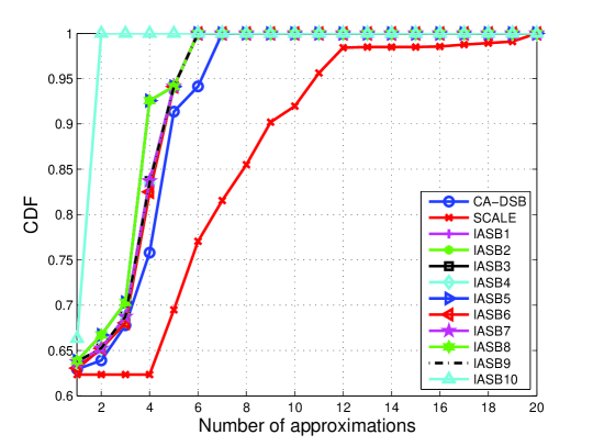
Figure 3: Cumulative distribution function (CDF) of the average number of approximations required to converge (averaged over all scenarios of Table II).

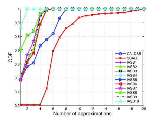
Figure 4: Cumulative distribution function (CDF) of the average number of approximations required to converge for scenario 7 of Table II

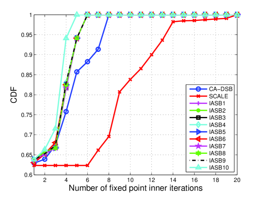
Figure 5: Cumulative distribution function (CDF) of the average number of fixed point updates required to converge (averaged over all scenarios of Table II).

The third column of Table III displays results for which the univariate approximations are solved up to accuracy $0.1~{}$dBm using a fixed point update approach (instead of using the closed-form formula). It can be seen that even when using the fixed point update approach, as highlighted in Section IV-E, the newly proposed methods show a significant improvement in convergence speed. All proposed methods perform better than existing methods, in particular IASB10. The CDF of the average number of fixed point updates (averaged over all DSL scenarios of Table II) is given in Figure 5 to highlight the variance between the methods. The same observations can be made as for the average number of approximations, except that the benefit of IASB10 compared to the other methods is no longer so large.

Finally, we would like to highlight that the ISB method in [40] is also an iterative per-user algorithm in which each subproblem is solved using an exhaustive search. The ISB algorithm however has two considerable disadvantages compared to the proposed methods: (i) solving a per-user subproblem with a simple exhaustive search requires much more computational effort, e.g., it takes several minutes of Matlab execution time to find the solution with ISB whereas only a few seconds are needed for the proposed methods. (ii) ISB considers a finite discrete granularity in transmit powers in contrast to the proposed methods, which negatively impacts the convergence speed.

V-B Improved Solution Quality

In this section we focus on the improved solution quality, i.e., improved data rate performance, when using the proposed iterative approximation methods with non-convex univariate approximations such as IASB3.

First we will demonstrate this starting from scenario 5 in Table II, which is a 6-user US VDSL scenario, and focusing on one particular (per-user per-tone) univariate approximation. In Figure 6 we plot the univariate approximations for user 5 on tone 600 for different methods, where we consider the per-user weighted achievable bit loading which corresponds to $-f_{600}^{\mathrm{app}}(s_{600}^{5};\mathbf{\tilde{s}}_{600}^{-5},\mathbf{\tilde{s}}_{600},\theta)$. The approximation point is chosen at the spectral mask -30 dBm. It can be seen that the CA-DSB, SCALE, IASB1 and IASB2 approximations get stuck in a bad locally optimal solution at -30 dBm when solved using the closed-form approach, whereas the nonconvex approximations of IASB3, IASB4 and IASB5 succeed in getting out of the bad locally optimal solution and result in the true global optimum at 0 dBm. In fact, IASB3 matches the original nonconvex objective. Note that we omit the plots of the IASB6, IASB7, IASB8, IASB9 and IASB10 approximations to avoid an overcrowded figure.

A second example focuses on scenario 8 of Table II, which is an important near-far 2-user DS ADSL setting for which it is known that it is difficult to find a good solution. In Table IV, we show the final achievable data rate performance of the IASB1 and IASB3 methods in terms of weighted achievable data rate sum as well as individual achievable data rates. Note that we choose non-equal weights for this scenario to prevent that the CO line of 5000m has a too small data rate performance, i.e., $w_{1}=1.2984$ and $w_{2}=0.1443$ which are normalized with $\log(2)$. Although the weighted achievable data rate sum is only slightly larger for IASB3, one can see that the individual achievable data rate $R^{2}$ of the RT-user is $7\%$ better while the CO-user’s achievable data rate $R^{1}$ is nearly unchanged. The reason for this improved solution quality is that the nonconvex approximations of IASB3 succeed in getting out of bad locally optimal solutions, resulting in an overall better achievable data rate performance. In Figure 7 the resulting transmit spectra are shown for both the CO- and RT-users and for both methods IASB1 and IASB3. A clear difference can be seen in the tone range 110 to 123, where IASB3 succeeds in obtaining better solutions with its nonconvex approximations, resulting in an overall improved solution quality.

TABLE IV: Comparison of solution quality for scenario 8 of Table II with IASB1 (using convex approximations) and IASB3 (using nonconvex approximations).

Performance measure	IASB1	IASB3
$w_{1}R^{1}+w_{2}R^{2}$ [Mbit/s]	$2.73~{}10^{6}$	$2.78~{}10^{6}$
$R^{1}$ [Mbit/s]	$1.60~{}10^{6}$	$1.59~{}10^{6}$
$R^{2}$ [Mbit/s]	$\mathbf{4.55~{}10^{6}}$	$\mathbf{4.87~{}10^{6}}$

We also want to highlight here that the improvement in solution quality obtained from the use of nonconvex approximations is only observed when using the closed-form solution approach, and is not obtained for the iterative fixed point update approach. For instance, for Figure 6, all methods would get stuck in -30 dBm when using the iterative fixed point update approach. This is an important advantage supporting the use of the closed-form solution approach with the proposed methods. Note however that for CA-DSB, SCALE and IASB10 the closed-form solution approach can not be used when considering scenarios with more than four users, as this requires computing the roots of some polynomials of degree larger than four, which is not always straightforward or even possible.

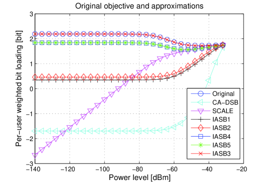
Figure 6: Original nonconvex per-user objective and its approximations

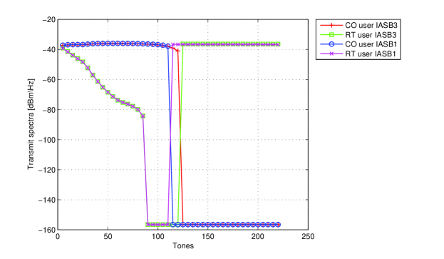
Figure 7: Transmit spectra scenario 8 from Table II using IASB1 and IASB3.

V-C Per-user Per-tone Selective Allocation of Approximations

As mentioned in Section IV-G, the proposed novel class of methods allows to exploit an extra degree of freedom that consists in allocating different approximations to different users and tones. For the per-user per-tone problems that are easy to approximate and convex, choosing a low-complexity approximation such as IASB1 and IASB6 is sufficient. Then again, other per-user per-tone problems may have a very nonconvex behaviour, with multiple local optima, for which it is more interesting to use nonconvex approximations, at the cost of solving a cubic equation instead of a simple linear equation.

Although it is not easy to determine which per-user per-tone problems are ’easy’, we can try to use some intuition. DSL scenarios can consist of mixed settings with CO-users and RT-users. These mixed settings are known to be scenarios with asymmetric crosstalk, i.e., the RT-users cause a lot of crosstalk to CO-users whereas the CO-users cause only minor crosstalk impact on the RT-users. From the univariate objective point of view, this translates to having simple univariate convex objective functions for the CO-users whereas having univariate non-convex objective functions for the RT-users. The connection between a small crosstalk level and convexity was also formally proven in [52]. For the CO-users the usage of convex approximations is good enough to converge to the univariate local optima, whereas for the RT-users one can benefit from nonconvex approximations to obtain an improved solution quality. We have performed simulations for the CO-RT scenario 8 of Table II where the IASB1 approximation is used for the CO-line of 5000m and the IASB3 approximation is used for the RT-line of 3000m. The resulting hybrid approach requires less computational effort compared to the IASB3 method, as the CO-user only has to solve polynomials of degree 1 instead of degree 3. The performance of the hybrid method is the same as that of the IASB3 method, i.e., superior to that of those based on convex approximations. One can thus have the same improved performance of IASB3 with a significantly decreased computational cost.

Similarly one can also make the approximations tone-dependent, i.e., frequency selective. For instance, the crosstalk is larger at high frequencies and one can expect that non-convex approximations may lead to better performance, in contrast to the low frequency bands with small crosstalk for which low complexity convex approximations are good enough. An optimized allocation of approximation types over different tones and users is an interesting topic for future research, but out of the scope of this paper.

V-D Choice of methods

Although a thorough trade-off analysis (theoretically as well as empirically) is conducted for the different proposed methods, such as the relation graph of Figure 1, it is not easy to give concrete recommendations on which method is the best. This is because this depends on the relative practical (hardware) cost of computing the solution of a polynomial of degree 1, 2 and 3. Furthermore the best choice depends on how much importance is given on preventing the method from getting stuck in bad locally optimal solutions. If solution quality is extremely important one should go for one of the nonconvex approximations, or a hybrid combination that takes the specific scenario into account as highlighted in Section V-C.

VI Conclusion

Multi-user multi-carrier systems that follow an interference channel based system model have become very important in practice. In such systems, the use of spectrum optimization can tackle the interference problem so as to spectacularly increase the achievable data rates. However this requires the development of efficient optimization methods to solve the corresponding nonconvex optimization problems. In this paper we demonstrate that existing spectrum optimization methods can be significantly improved when taking their typical per-user implementation explicitly into account at the early design stage. Applying this concept, we derived a novel class of iterative approximation methods which focuses on efficiently solvable univariate approximations, instead of the jointly convex approximations of existing methods (CA-DSB and SCALE). For this novel class, a design framework is proposed that can be used to construct improved approximations that are much tighter than existing approximations and that can be solved in closed-form, in contrast to existing methods that require iterative fixed point updates. As a result, methods belonging to this novel class both converge in fewer iterations and require fewer computations per iteration. Using this design framework, we construct ten novel methods referred to as IASB1 up to IASB10, and analyze and discuss their improved tightness and reduced computational cost. Methods IASB1, IASB2 and IASB6 involve convex univariate approximations, whereas the other methods rely on nonconvex univariate approximations. Extensive simulations using a realistic multi-user DSL simulator demonstrate a factor 2 to 4 improvement in convergence speed, while decreasing the computational cost per iteration. Furthermore the methods using nonconvex approximations somehow allow to tackle nonconvexity of the optimization problem: since they allow escape from bad locally optimal solutions, they can improve solution quality compared to existing methods, which is demonstrated for IASB3, IASB4 and IASB5. In particular, methods using multiple reference lines, namely IASB5, IASB8 as well as IASB10, perform very well in terms of their trade-off between computational cost, convergence speed and solution quality. Finally it is shown that the proposed algorithm permits the selection of different approximations over different users and tones, which allows for further performance improvements, as demonstrated for a mixed DSL setting.

References

- [1] P. Tsiaflakis and F. Glineur, “A novel class of iterative approximation methods for DSL spectrum optimization,” in Proc. of the IEEE International Conference on Communications, Ottawa, Canada, June 2012, pp. 1–6.
- [2] D. Gesbert, S. Hanly, H. Huang, S. S. Shitz, O. Simeone, and W. Yu, “Multi-cell mimo cooperative networks: A new look at interference,” IEEE Journal on Selected Areas in Communications, vol. 28, no. 9, pp. 1380–1408, Dec. 2010.
- [3] R. Cendrillon, W. Yu, M. Moonen, J. Verlinden, and T. Bostoen, “Optimal multiuser spectrum balancing for digital subscriber lines,” IEEE Transactions on Communications, vol. 54, no. 5, pp. 922–933, May 2006.
- [4] M. Wolkerstorfer, D. Statovci, and T. Nordström, “Dynamic spectrum management for energy-efficient transmission in DSL,” in Proc. of the Eleventh IEEE International Conference on Communications Systems, China, Nov. 2008.
- [5] M. Monteiro, N. Lindqvist, and A. Klautau, “Spectrum balancing algorithms for power minimization in DSL networks,” in Proc. of the IEEE International Conference on Communications, Dresden, Germany, Jun. 2009, pp. 1–5.
- [6] P. Tsiaflakis, Y. Yi, M. Chiang, and M. Moonen, “Fair greening of broadband access: spectrum management for energy-efficient DSL networks,” EURASIP Journal on Wireless Communications and Networking, vol. 2011:140, 2011.
- [7] D. Würtz, A. Klein, and M. Kuipers, “Distributed margin optimization using spectrum balancing in multi-user DSL systems,” in 20th European Signal Processing Conference, Bucharest, Romania, Aug. 2012, pp. 1–5.
- [8] M. Monteiro, A. Gomes, N. Lindqvist, B. Dortschy, and A. Klautau, “An algorithm for improved stability of DSL networks using spectrum balancing,” in Proc. of the IEEE Global Telecommunications Conference, Miami, Florida, USA, Dec. 2010, pp. 1–6.
- [9] T. Han and K. Kobayashi, “A new achievable rate region for the interference channel,” IEEE Transactions on Information Theory, vol. 27, no. 1, pp. 49–60, Jan. 1981.
- [10] H. Sato, “The capacity of the gaussian interference channel under strong interference,” IEEE Transactions on Information Theory, vol. 27, no. 6, pp. 786–788, 1981.
- [11] C. Sung, K. Lui, K. Shum, and H. So, “Sum capacity of one-sided parallel gaussian interference channels,” IEEE Transactions on Information Theory, vol. 54, no. 1, pp. 468–472, Jan. 2008.
- [12] N. Liu and S. Ulukus, “The capacity region of a class of discrete degraded interference channels,” IEEE Transactions on Information Theory, vol. 54, no. 9, pp. 4372–4378, Sep. 2008.
- [13] H.-F. Chong, M. Motani, H. K. Garg, and H. E. Gamal, “On the han-kobayashi region for the interference channel,” IEEE Transactions on Information Theory, vol. 54, no. 7, pp. 3188–3195, Jul. 2008.
- [14] G. Kramer, “Outer bounds on the capacity of gaussian interference channels,” IEEE Transactions on Information Theory, vol. 50, no. 3, pp. 581–586, Mar. 2004.
- [15] R. Etkin, D. Tse, and H. Wang, “Gaussian interference channel capacity to within one bit,” IEEE Transactions on Information Theory, vol. 54, no. 12, pp. 5534–5562, Dec. 2008.
- [16] X. Shang, G. Kramer, and B. Chen, “A new outer bound and the noisy-interference sum-rate capacity for gaussian interference channels,” IEEE Transactions on Information Theory, vol. 55, no. 2, pp. 689–699, Feb. 2009.
- [17] M. Chiang, C. Tan, D. Palomar, D. O’Neill, and D. Julian, “Power control by geometric programming,” IEEE Transactions on Wireless Communications, vol. 6, no. 7, pp. 2640–2651, Jul. 207.
- [18] M. Chiang, P. Hande, T. Lan, and C. Tan, “Power control in wireless cellular networks,” Foundations and Trends in Networking, vol. 2, no. 4, pp. 381–533, 2008.
- [19] S. Haykin, “Cognitive radio: brain-empowered wireless communications,” IEEE Journal on Selected Areas in Communications, vol. 23, no. 2, pp. 201–220, 2005.
- [20] V. Chandrasekhar, J. G. Andrews, T. Muharemovic, Z. Shen, and A. Gatherer, “Power control in two-tier femtocell networks,” IEEE Transactions on Wireless Communications, vol. 8, no. 8, pp. 4316–4328, Aug 2009.
- [21] G. Aristomenopoulos, T. Kastrinogiannis, S. Lamprinakou, and S. Papavassiliou, “Optimal power control and coverage management in two-tier femtocell networks,” EURASIP Journal on Wireless Communications and Networking, vol. 2012:329, 2012.
- [22] C. Tan, S. Friedl, and S. H. Low, “Spectrum management in multiuser cognitive wireless networks: Optimality and algorithm,” IEEE Journal on Selected Areas in Communications, vol. 29, no. 2, pp. 421–430, Feb. 2011.
- [23] P. Weeraddana, M. Codreanu, M. Latva-aho, and A. Ephremides, “Weighted sum-rate maximization for a set of interfering links via branch and bound,” IEEE Transactions on Signal Processing, vol. 59, no. 8, pp. 3977–3996, Aug. 2011.
- [24] Z. Jing, B. Bai, and X. Ma, “Price-based interference avoidance game in the gaussian interference channel,” Science China Information Sciences, vol. 55, no. 2, pp. 301–311, 2012.
- [25] Y. Zhao and G. J. Pottie, “Optimal spectrum management in multiuser interference channels,” in Proc. of the IEEE International Symposium on Information Theory, Seoul, Korea, Jun. 2009, pp. 2266–2270.
- [26] S. Ren and M. van der Schaar, “Distributed power allocation in multi-user multi-channel cellular relay networks,” IEEE Transactions on Wireless Communications, vol. 9, no. 6, pp. 1952–1964, Jun. 2010.
- [27] K. Son, S. Lee, Y. Yi, and S. Chong, “REFIM: A practical interference management in heterogeneous wireless access networks,” IEEE Journal on Selected Areas in Communications, vol. 29, no. 6, pp. 1260–1272, Jun. 2011.
- [28] P. Weeraddana, M. Codreanu, M. Latva-aho, and A. Ephremides, “Resource allocation for cross-layer utility maximization in wireless networks,” IEEE Transactions on Vehicular Technology, vol. 60, no. 6, pp. 2790–2809, Jul. 2011.
- [29] P. Tsiaflakis, Y. Yi, M. Chiang, and M. Moonen, “Throughput and delay of DSL dynamic spectrum management with dynamic arrivals,” in Proc. of the IEEE Global Telecommunications Conference, Nov. 2008, pp. 1–5.
- [30] ——, “Throughput and delay performance of DSL broadband access with cross-layer dynamic spectrum management,” IEEE Transactions on Communications, vol. 60, no. 9, pp. 2700–2711, Sep. 2012.
- [31] R. Cendrillon, J. Huang, M. Chiang, and M. Moonen, “Autonomous spectrum balancing for digital subscriber lines,” IEEE Transactions on Signal Processing, vol. 55, no. 8, pp. 4241–4257, Aug. 2007.
- [32] P. Tsiaflakis, M. Diehl, and M. Moonen, “Distributed spectrum management algorithms for multiuser DSL networks,” IEEE Transactions on Signal Processing, vol. 56, no. 10, pp. 4825–4843, Oct. 2008.
- [33] C. Leung, S. Huberman, and T. Le-Ngoc, “Autonomous spectrum balancing using multiple reference lines for digital subscriber lines,” in Proc. of IEEE Global Telecommunications Conference, Houston, TX, December 2010.
- [34] W. Yu, “Multiuser water-filling in the presence of crosstalk,” in Information Theory and Applications (ITA), San Diego, USA, Feb. 2007.
- [35] J. Papandriopoulos and J. S. Evans, “SCALE: A low-complexity distributed protocol for spectrum balancing in multiuser DSL networks,” IEEE Transactions on Information Theory, vol. 55, no. 8, pp. 3711–3724, Aug. 2009.
- [36] R. B. Moraes and J. R. i. R. B. Dortschy, A. Klautau, “Semiblind spectrum balancing for DSL,” IEEE Transactions on Signal Processing, vol. 58, no. 7, pp. 3717–3727, Jul. 2010.
- [37] T. Wang and L. Vandendorpe, “Successive convex approximation based methods for dynamic spectrum management,” in Proc. of the IEEE International Conference on Communications, Ottawa, Canada, Jun. 2012.
- [38] Y. Xu, T. Le-Ngoc, and S. Panigrahi, “Global concave minimization for optimal spectrum balancing in multi-user DSL networks,” IEEE Trans. on Signal Processing, vol. 56, no. 7, pp. pp. 2875–2885, Jul. 2008.
- [39] P. Tsiaflakis, J. Vangorp, M. Moonen, and J. Verlinden, “A low complexity optimal spectrum balancing algorithm for digital subscriber lines,” Signal Processing, vol. 87, no. 7, pp. 1735–1753, Jul. 2007.
- [40] R. Cendrillon and M. Moonen, “Iterative spectrum balancing for digital subscriber lines,” in Proc. of the IEEE International Conference on Communications, vol. 3, no. 3, May 2005, pp. 1937–1941.
- [41] W. Yu and R. Lui, “Dual methods for nonconvex spectrum optimization of multicarrier systems,” IEEE Transactions on Communications, vol. 54, no. 7, Jul. 2006.
- [42] M. Wolkerstorfer, J. Jalden, and T. Nordström, “Low-complexity optimal discrete-rate spectrum balancing in digital subscriber lines,” Signal Processing, pp. 1–12, Jun. 2012.
- [43] Z. Q. Luo and S. Zhang, “Duality gap estimation and polynomial time approximation for optimal spectrum management,” IEEE Transactions on Signal Processing, vol. 57, no. 7, pp. 2675–2689, Jul. 2009.
- [44] P. Tsiaflakis, J. Vangorp, M. Moonen, and J. Verlinden, “Convex relaxation based low-complexity optimal spectrum balancing for multi-user DSL,” in Proceedings of IEEE International Conference on Acoustics, Speech and Signal Processing, vol. 3, Apr. 2007, pp. III–349 – III–352.
- [45] S. Huberman, C. Leung, and T. Le-Ngoc, “Dynamic spectrum management (dsm) algorithms for multi-user xDSL,” IEEE Communications Surveys and Tutorials, vol. 14, no. 1, First quarter 2012.
- [46] K. Kerpez, “Near-end crosstalk is almost gaussian,” IEEE Transactions on Communications, vol. 41, no. 5, pp. 670–672, May 1993.
- [47] T. Starr, J. M. Cioffi, and P. J. Silverman, Understanding digital subscriber lines. Prentice Hall, 1999.
- [48] B. Marks and G. Wright, “A general inner approximation algorithm for nonconvex mathematical programs,” Operations Research, vol. 26, no. 4, pp. 681–683, 1978.
- [49] Z. Q. Luo and S. Zhang, “Dynamic spectrum management: Complexity and duality,” IEEE Journal of Selected Topics in Signal Processing, vol. 2, no. 1, pp. 57–73, Feb. 2008.
- [50] “Spectrum management for loop transmission systems,” ANSI, Tech. Rep. T1.417, Issue 2, 2003.
- [51] “Transmission and Multiplexing (TM); Access transmission systems on metallic access cables; Very high speed Digital Subscriber Line (VDSL); Functional Requirements,” ETSI, Tech. Rep., 2003.
- [52] P. Tsiaflakis, C. W. Tan, Y. Yi, M. Chiang, and M. Moonen, “Optimality certificate of dynamic spectrum management in multi-carrier interference channels,” in Proc. of the IEEE International Symposium on Information Theory, Jul. 2008, pp. 1298–1302.