Hot methane line lists for exoplanet and brown dwarf atmospheres
(CORRECTED )

Abstract

We present comprehensive experimental line lists of methane (CH₄) at high temperatures obtained by recording Fourier transform infrared emission spectra. Calibrated line lists are presented for the temperatures 300 – 1400^∘C at twelve 100^∘C intervals spanning the 960 – 5000 cm^-1 (2.0 – 10.4 $\mu$m) region of the infrared. This range encompasses the dyad, pentad and octad regions, i.e., all fundamental vibrational modes along with a number of combination, overtone and hot bands. Using our CH₄ spectra, we have estimated empirical lower state energies ($E_{low}$ in cm^-1) and our values have been incorporated into the line lists along with line positions ($\tilde{\nu}$ in cm^-1) and calibrated line intensities ($S^{\prime}$ in cm molecule^-1). We expect our hot CH₄ line lists to find direct application in the modeling of planetary atmospheres and brown dwarfs.

1 INTRODUCTION

Methane (CH₄) is the most fundamental alkane molecule and is second only to CO₂ in causing climate change (IPCC, 2007). The presence of CH₄ in the Earth’s atmosphere is a consequence of both anthropogenic (e.g., landfills, rice cultivation, waste water treatment) and natural sources (e.g., methanogens, wetlands, wildfires). CH₄ can also be found throughout the solar system (Karkoschka, 1994) including the atmospheres of Jupiter, Saturn, Uranus, Neptune and tentatively in the Martian atmosphere (Mumma et al., 2009). Titan, the largest moon of Saturn, has a dense atmosphere which is mostly made up of nitrogen but contains a relatively large proportion of CH₄ (approximately 1.4% in the stratosphere; Niemann et al. 2005). The concentration of CH₄ is higher near the surface and it is believed a methane cycle exists which leads to the formation of liquid CH₄ lakes (Stofan et al., 2007). Interestingly, CH₄ has also been observed in the spectral energy distributions (SEDs) of cool substellar objects such as brown dwarfs (Cushing et al., 2006) and more recently in exoplanet atmospheres (Swain et al., 2008; Seager & Deming, 2010).

Cool stars and brown dwarfs are classified according to the molecular features in the observed SED (Bernath, 2009). The cooler the object, the more molecular signatures can be identified in the SED (Kirkpatrick, 2005). L dwarfs display near-infrared electronic transitions of metal hydrides such as FeH (Hargreaves et al., 2010) and weaker TiO and VO bands (Geballe et al., 2002) which are more commonly associated with M dwarfs (Leggett et al., 2001; Bernath, 2009). T dwarfs contain significant absorption due to H₂O and CH₄ (Cushing et al., 2006) and have been referred to as ‘methane dwarfs’ (Hauschildt et al., 2009) because methane is the characteristic absorber. The newest category of brown dwarf (Y class) has recently been observed (Cushing et al., 2011) and displays characteristic NH₃ absorptions along with additional CH₄ absorption. Given these band assignments, the SEDs of brown dwarfs are complex and still contain numerous unassigned features.

The study of exoplanets is relatively new, as it was not until the mid-1990s that the first exoplanet was discovered (Mayor & Queloz, 1995). In recent years, ‘hot-Jupiters’ are being discovered at an increasing rate and Kirkpatrick et al. (2011) were able to identify a further 100 using NASA’s Wide-field Infrared Survey Explorer. It is now possible to probe the atmospheres of exoplanets (Charbonneau et al., 2002) by utilizing the natural transit as the planet passes in front of its parent star. The resulting flux undergoes a characteristic ‘dip’ at specific wavelengths during the planetary transit (Charbonneau et al., 2000) and from the extremely small variations in the wavelength dependence of the dips it is possible to determine which molecules are present. By utilizing the transit method, H₂O (Barman, 2008; Grillmair et al., 2008), CH₄ (Swain et al., 2008), CO (Swain et al., 2009b) and CO₂ (Swain et al., 2009a; Tinetti et al., 2010) have already been identified. Currently this method has only been successful for large hot-Jupiters, but NASA’s Kepler mission is discovering ever smaller planets which more closely resemble Earth, such as Kepler-22b (Borucki et al., 2012). Exoplanets are now thought to be the rule, rather than the exception, throughout the Milky Way (Cassan et al., 2012) and the ultimate exoplanet goal is to detect the distinctive signatures of extra terrestrial life through observation of the atmospheres of these distant planets.

Table 1: The fundamental infrared modes of CH₄

Mode	Degeneracy	Band Origin (cm-1)	Type
$\nu_{1}$ $(a_{1})$	1	2916.481	Symmetric C–H Stretch
$\nu_{2}$ $(e)$	2	1533.333	Bend
$\nu_{3}$ $(t_{2})$	3	3019.493	Antisymmetric C–H Stretch
$\nu_{4}$ $(t_{2})$	3	1310.761	Bend

Infrared spectroscopy of CH₄ is complex due to the high symmetry of the molecule and the polyad structure which arises from close-lying vibrational levels (Boudon et al., 2006). CH₄ is a tetrahedral molecule (T_d symmetry) and is a classic example of a spherical top. There are $3N-6=9$ infrared modes with four stretches and five bends. The four C–H stretches correspond to a symmetric $a_{1}$ stretch ($\nu_{1}$ at 2916.481 cm^-1) and a triply degenerate $t_{2}$ antisymmetric stretch ($\nu_{3}$ at 3019.493 cm^-1). The five bends correspond to a doubly degenerate $e$ bending mode ($\nu_{2}$ at 1533.333 cm^-1) and a triply degenerate $t_{2}$ bending mode ($\nu_{4}$ at 1310.761 cm^-1). The spectroscopic constants of CH₄ are summarised in Table 1 (Albert et al., 2009; Herzberg, 1991) and only the $\nu_{3}$ and $\nu_{4}$ fundamental modes are nominally infrared active; however, it is possible for other modes to gain intensity through strong interactions within the polyad structure. The interesting polyad structure of the infrared spectrum of CH₄ arises because the bending frequencies are approximately equal ($\nu_{2}\approx\nu_{4}$), the stretching frequencies are also approximately equal ($\nu_{1}\approx\nu_{3}$) and approximately twice the bending frequencies (Albert et al., 2009). For example, the pentad region near 3 $\mu$m has 5 vibrational bands since $\nu_{1}\approx\nu_{3}\approx 2\nu_{2}\approx 2\nu_{4}\approx\nu_{2}+\nu_{4}$.

CH₄ has also frequently been the target of high quality theoretical calculations based on the solution of the vibration-rotation Schrödinger equation (Wang & Sibert, 2002; Wang & Carrington, 2004; Cassam-Chenaï, 2003) using ab initio potential energy surfaces (Schwenke & Partridge, 2001; Schwenke, 2002; Nikitin et al., 2011). The accuracy of vibration-rotational calculations are typically far from experiment; however, recent calculations of nominally forbidden pure rotational lines (Cassam-Chenaï & Liévin, 2012) are able to approach experimental accuracy.

Albert et al. (2009) have reported a study of CH₄ in the 0 – 4800 cm^-1 region and these lines form the basis of the HITRAN 2008 database (Rothman et al., 2009). Extensive work has been carried out in Grenoble including the preparation of a cold CH₄ line list (Mondelain et al., 2011; Wang et al., 2011, 2012; Campargue et al., 2012a) which has been successfully applied to the atmosphere of Titan (Campargue et al., 2012b). Recently focus has shifted to the generation of hot line lists for use in brown dwarfs and exoplanet models, either from ab initio calculations (Warmbier et al., 2009) or from experiment (Nassar & Bernath, 2003; Perrin & Soufiani, 2007; Thiévin et al., 2008).

Radiative transfer models are typically used to identify molecules in the atmospheres of exoplanets (Swain et al., 2008). Adaptations for hot-Jupiter atmospheres include known strongly absorbing molecules (i.e. H₂O and CH₄) and one of the options for CH₄ has been the HITRAN 2008 database (Rothman et al., 2009) combined with experimental data obtained by Nassar & Bernath (2003). HITRAN covers a broad spectral range but is intended for room temperature applications whereas the Nassar & Bernath (2003) data are only recorded at three higher temperatures (800, 1000 and 1273 K). This limits the accuracy of the modeled SEDs and leads to errors in deriving effective temperatures (Hauschildt et al., 2009). We hope to address this issue by providing a series of high-resolution, hot CH₄ line lists at temperatures relevant to exoplanet and brown dwarf atmospheres with the inclusion of empirical lower state energies where possible. This work will cover the dyad ($\nu_{2}$, $\nu_{4}$), pentad ($\nu_{1}$, $\nu_{3}$, $2\nu_{2}$, $2\nu_{4}$, $\nu_{2}+\nu_{4}$) and octad ($3\nu_{2}$, $3\nu_{4}$, $\nu_{1}+\nu_{2}$, $\nu_{1}+\nu_{4}$, $\nu_{3}+\nu_{2}$, $\nu_{3}+\nu_{4}$, $2\nu_{2}+\nu_{4}$, $\nu_{2}+2\nu_{4}$) regions of the infrared including numerous hot bands. Similar work has already been carried out on NH₃ (Hargreaves et al., 2011, 2012). Our data sets, and molecular opacities derived from them, can be used directly in exoplanet and brown dwarf models.

2 EXPERIMENTAL METHOD

High-resolution laboratory emission spectra of hot CH₄ were recorded in four separate parts in order to maximise the signal-to-noise for each spectral region. The four spectral regions are shown in Figure 1 for 1000^∘C. A similar setup was used in our previous work on NH₃ (Hargreaves et al., 2011, 2012) and only key experimental features will be summarized here.

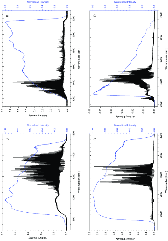
Figure 1: High-resolution laboratory emission spectra of CH₄ at 1000^∘C for all four regions (black) with the corresponding normalized instrument response function (blue). The baseline is caused by residual thermal emission from the tube walls and a small amount of absorption due to cold CH₄, CO₂ ($\nu_{3}$ near 2350 cm^-1) and H₂O can be seen.

The experiment coupled a Fourier transform infrared (FT-IR) spectrometer with a temperature controllable tube furnace capable of maintaining stable temperatures up to 1400^∘C with an accuracy $\pm 10^{\circ}$C. The tube furnace surrounds the central portion of an alumina (Al₂O₃) tube which is sealed at both ends by infrared windows. CH₄ gas is allowed to flow through the alumina tube at a stable pressure in order to avoid the build up of impurities. The infrared emission from the alumina tube was focussed onto the aperture of the FT-IR spectrometer using a lens. The small region between the spectrometer and tube furnace was purged with dry air in order to minimize H₂O absorption lines in the recorded spectra. Table 2 contains the experimental parameters used for all four regions.

Table 2: Experimental conditions

	Region A	Region B	Region C	Region D
Total file coverage (cm-1)	600–1900	1000–3000	1500–5000	2500–8000
Temperature Range (∘C)	300–1400	300–1400	300–1400	500–1300
Detector	MCT	MCT	InSb	InSb
Beam Splitter	KBr	CaF2	CaF2	CaF2
Windows	KRS-5	CaF2	CaF2	CaF2
Lens	ZnSe	CaF2	CaF2	CaF2
Total scans	240	300	300	800
Resolution (cm-1)	0.01	0.015	0.015	0.02
Aperture (mm)	2.5	2.5	2.5	1.7
CH4 pressure (Torr)	4.0	4.0	4.0	60.0
Zero-fill factor	$\times 16$	$\times 16$	$\times 16$	$\times 16$

Spectra were recorded at 100^∘C intervals between 300 and 1400^∘C for regions A, B and C and between 500 and 1300^∘C for region D as this was the temperature coverage of observable CH₄ emission. Each region was limited using an appropriate filter chosen to allow for overlap between neighbouring regions. The resolution of each spectral region was based on the Doppler and pressure broadening widths, and was selected to minimize the acquisition time whilst maintaining the maximum line resolution.

The temperature of the tube furnace was measured and maintained at high temperatures using a thermocouple combined with a programmable controller. The ends of the alumina tube required cooling to avoid damaging the rubber o-rings (which maintain the pressure seal) and the consequence of this is a temperature gradient within the tube. The observed infrared emission spectra are dominated by the high temperature central portion of the tube (see Figure 1) and the emission lines are assumed to be formed at the same temperature as the furnace.

The emission lines in each spectrum were picked using the program WSpectra (Carleer, 2001) and the line intensity of each line was obtained by fitting a Voigt line profile. The number of CH₄ emission lines recorded for each region is given in Table 3.

Table 3: Observed emission lines of CH₄

Temperature (∘C)	Region A	Region B	Region C	Region D	Total
300	4,365	2,589	4,118	-	11,072
400	6,656	3,566	7,752	-	17,974
500	7,950	4,725	9,438	5,242	27,355
600	9,524	6,021	14,109	7,766	37,420
700	10,381	6,344	15,376	10,067	42,168
800	11,189	6,951	19,297	12,696	50,133
900	11,607	7,276	21,148	14,688	54,719
1000	12,005	7,889	21,042	16,563	57,499
1100	12,105	7,667	21,850	16,062	57,684
1200	12,368	7,637	22,511	10,269	52,785
1300	12,235	8,118	23,332	9,640	53,325
1400	12,510	6,095	10,590	-	29,195

A system response function was measured for each region by recording a blackbody spectrum emitted from a graphite rod placed at the centre of the the alumina tube (i.e., at the centre of the furnace). This accounts for the relative contribution of the system (e.g., windows, lens, filters, etc.) to the intensity of the observed lines. The spectrum is compared to a theoretical blackbody at the temperature of the furnace and then normalized. These instrument response functions are shown in Figure 1 along with the CH₄ emission lines at 1000^∘C.

It was necessary to calibrate both the wavenumber scale ($x$-axis) and the intensity scale ($y$-axis) using the HITRAN line list. The wavenumber scales were calibrated by selecting 20 strong, clear, symmetric lines and averaging the correction factor. Each temperature spectrum had similar calibration factors and typical values (for the 1000^∘C spectra) were 1.000001351 for region A, 1.000001677 for region B, 1.000001051 for region C and 1.000000091 for region D. This results in a typical shift of 0.005 cm^-1 at 3000 cm^-1 for the $\nu_{3}$ band. We therefore expect the accuracy of each each line list to be $\pm$0.005 cm^-1 or better.

The intensity scales have also been calibrated according to HITRAN. First, each emission line list was converted into an arbitrary absorption scale to make them comparable to the intensities of the lines contained in HITRAN. This method has previously been used by Nassar & Bernath (2003) and more recently by Hargreaves et al. (2011, 2012) by using the equation

$$S_{a}=\frac{S_{e}}{\nu^{3}\exp\left(-\frac{h\nu}{kT}\right)},$$ (1)

where $S_{a}$/$S_{e}$ is the intensity of the absorbed/emitted line, $\nu$ is the frequency and $T$ is the temperature.

Each line list was then put onto the same intensity scale as recorded by region A, and comparisons to HITRAN were made. The HITRAN lines had to be scaled to the appropriate temperatures using

$$S^{\prime}=S^{\prime}_{0}\frac{Q_{0}}{Q}\exp\left(\frac{E_{low}}{kT_{0}}-\frac{E_{low}}{kT}\right)\left[\frac{1-\exp\left(-\frac{h\nu_{10}}{kT}\right)}{1-\exp\left(-\frac{h\nu_{10}}{kT_{0}}\right)}\right],$$ (2)

where $S^{\prime}$ is the intensity, $Q$ is the partition function, $T$ is the temperature, $\nu_{10}$ is the line frequency and $E_{low}$ is the empirical lower state energy (Bernath, 2005). A zero subscript refers to the same parameters but at the reference temperature. The partition functions can be found in Table 4 and were calculated for each temperature using the TIPS$\_$2011.for program (Laraia et al., 2011) based on calculations made by Wenger et al. (2008).

Table 4: Methane partition function

Temperature (K)	Partition Function
296	590.52
573	1,856.19
673	2,648.82
773	3,745.99
873	5,267.13
973	7,372.47
1073	10,276.30
1173	14,266.42
1273	19,723.43
1373	27,161.91
1473	37,273.63
1573	50,996.68
1673	69,611.60

Wavenumber matches between our data and the temperature-scaled HITRAN lines were made ($\pm$0.005 cm^-1) and these intensities were compared. A calibrating factor could then be deduced but as the frequency increased, the intensity calibration factors became larger and more inconsistent. Regions A, B, and C could all be matched without difficulty since these regions cover strong emission bands; however, region D proved to be a problem. In the end, it was decided that an intensity calibration function could be extrapolated into region D based on the matches from regions A, B and C. The intensity calibration used to convert the observed arbitrary intensity ($S^{\prime}_{arb}$) to intensities in HITRAN units ($S^{\prime}_{H}$) is

$$S^{\prime}_{H}=[a(\tilde{\nu})^{2}+b\tilde{\nu}+c]S^{\prime}_{arb},$$ (3)

where $\tilde{\nu}$ is in cm^-1 and $S^{\prime}_{H}$ is in cm molecule^-1. The calibration function is temperature dependent and was applied to all regions, the constants are given in Table 5.

Table 5: Wavenumber calibration functions

Temperature	$a$	$b$	$c$
(∘C)	(/$10^{12}$ cm3 molecule-1)	(/$10^{15}$ cm2 molecule-1)	(/$10^{18}$ cm molecule-1)
300	2.92	-9.75	12.00
400	1.48	-2.15	4.98
500	2.82	-6.67	9.03
600	3.62	-9.87	12.30
700	4.04	-10.70	13.30
800	2.56	-3.35	6.02
900	3.24	-6.17	8.63
1000	4.87	-12.40	14.20
1100	4.00	-7.77	9.33
1200	4.07	-7.18	7.95
1300	5.06	-12.00	12.60
1400	4.68	-7.48	7.29

Each region had to be combined to form a complete line list at each temperature. The optical filters used during the acquisition of each spectrum allowed the regions to overlap; the common lines in the overlapping regions have been used to bring all regions onto the same scale. The number of emission lines in the final line lists were maximized by appropriately choosing to combine the regions at 1500, 1830 and 3350 cm^-1. Because emission lines were only recorded above 960 cm^-1 and region D was intentionally truncated at 5000 cm^-1, the spectral regions are 960 – 1500 cm^-1 (region A), 1500 – 1830 cm^-1 (region B), 1830 – 3350 cm^-1 (region C) and 3350 – 5000 cm^-1 (region D), i.e., 960 – 5000 cm^-1 in total.

The emission lines for each temperature were compared to all other temperatures and all matchable lines were identified ($\pm$0.005 cm^-1). It is then possible to calculate the empirical lower state energy ($E_{low}$) of each line by rearranging Equation 2 so that

$$\ln\left(\frac{SQR_{0}}{S_{0}Q_{0}R}\right)=\frac{E_{low}}{kT_{0}}-\frac{E_{low}}{kT},$$ (4)

where

$$R_{0}={1-\exp\left(-\frac{h\nu_{10}}{kT_{0}}\right)}.$$ (5)

The slope of points plotted using Equation (4) for each line yields the $E_{low}$ and an example of this calculation is shown in Figure 2 for five CH₄ emission lines present at all temperatures.

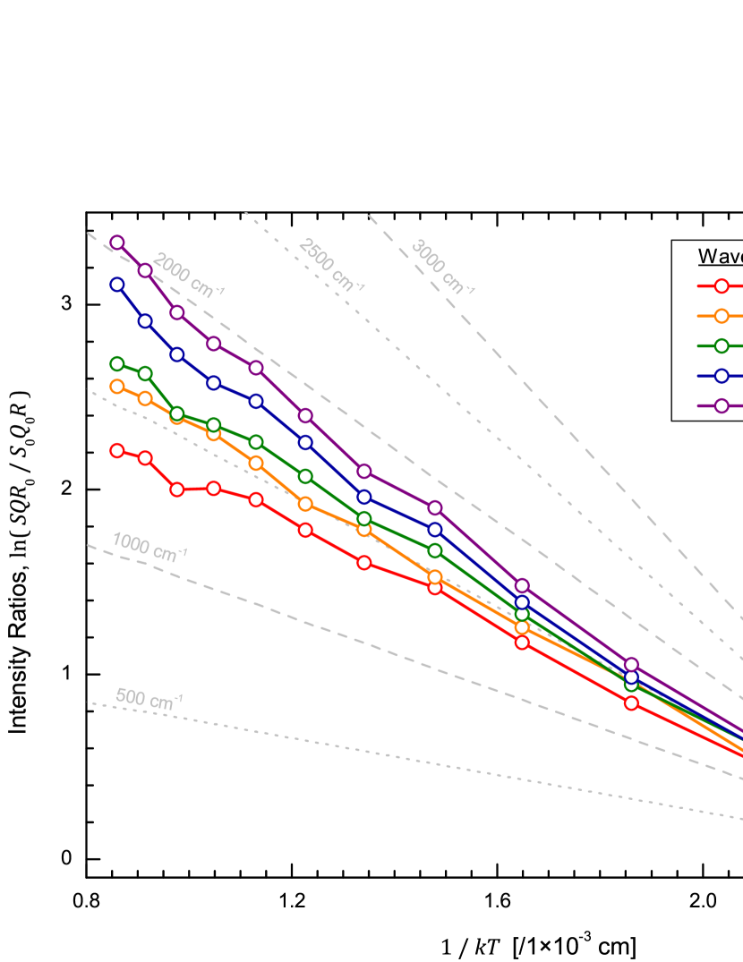
Figure 2: Natural logarithm of the intensity ratios of five lines present in all 12 spectra are plotted against $1/kT$ (in cm), where $T$ is the temperature. The slope of each line directly yields the empirical lower state energy (in cm^-1) and for the lines plotted: $E_{low}[1]=1364.00$ cm^-1 (red), $E_{low}[2]=1590.79$ cm^-1 (orange), $E_{low}[3]=1644.41$ cm^-1 (green), $E_{low}[4]=1879.95$ cm^-1 (blue), and $E_{low}[5]=2036.83$ cm^-1 (purple).

This then forms the basis of the temperature dependant line lists which contain calibrated line positions ($\tilde{\nu}$ in cm^-1), calibrated line intensities ($S^{\prime}$ in cm/molecule) and empirical lower state energies ($E_{low}$ in cm^-1). It was necessary to incorporate missing HITRAN lines into these line lists as explained in the results.

3 RESULTS

Using our method to calculate the $E_{low}$ values, it is possible to identify the dyad, pentad and octad infrared regions of CH₄ in the plots of $E_{low}$ versus wavenumber (Figure 3).

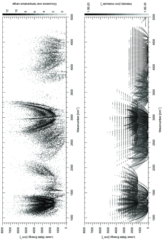
Figure 3: Comparison of the empirical lower state energies (top panel) with the HITRAN lower state energies (bottom panel). The dyad ($\nu_{4}$ region), pentad ($\nu_{3}$ region) and octad ($\nu_{3}+\nu_{4}$) regions are clearly visible.

The two most striking features are the $\nu_{4}$ region (dyad) around 1300 cm^-1 and the $\nu_{3}$ region (pentad) around 3020 cm^-1. The $\nu_{4}$ region contains lines of the fundamental $\nu_{4}$ bend and distinct $2\nu_{4}-\nu_{4}$ and $3\nu_{4}-2\nu_{4}$ hot bands at a $E_{low}$ of 1300 and 2600 cm^-1 respectively. The $\nu_{3}$ region contains a strong $P$-, $Q$-, and $R$-branch of the $\nu_{3}+\nu_{4}-\nu_{4}$ hot band above a $E_{low}$ of 1300 cm^-1 and parts of the fundamental $P$-, and $R$-branch of the $\nu_{3}$ mode. Another hot band, possibly the $2\nu_{3}-\nu_{3}$, can be seen above a $E_{low}$ of $\sim$3000 cm^-1. Less obvious but still present are tentative observations of the $Q$-branch of the ‘forbidden’ $\nu_{2}$ fundamental bend at approximately 1530 cm^-1. Also present are features of the $\nu_{3}+\nu_{4}$ combination region (octad) around 4300 cm^-1, although the features in this region are less distinct as it is congested by many other bands. Comparisons to HITRAN for this region shows a complex band structure as expected due to the high density of transitions.

There is reasonable agreement between the empirical $E_{low}$ values and the HITRAN $E_{low}$ values (Figure 3) within the $\nu_{3}$ and $\nu_{4}$ region. A hot band at a lower state energy of approximately 3000 cm^-1 in the pentad region (tentatively assigned the $2\nu_{3}-\nu_{3}$ hot band) is absent in HITRAN and is not very well defined in our data. We have observed emission lines with higher rotational levels than are present in HITRAN which is most apparent in the vicinity of the $\nu_{3}$ region. The HITRAN database clearly contains many CH₄ lines, but the majority of $E_{low}$ values have been obtained from calculations; these $E_{low}$ values are visible in Figure 3 as horizontal ‘stripes’ which correspond to the distinct rotational levels.

Our method is also able to distinguish rotational structure of the branches of the $\nu_{3}$ fundamental mode as shown in Figure 4. The rotational levels of a rigid spherical top are given by $BJ(J+1)$ but there is a $(2J+1)^{2}$-fold degeneracy for each $J$ (i.e., $(2J+1)$ from the $M$ quantum number and $(2J+1)$ from $K$). As the molecule rotates and distorts, the $K$ degeneracy is partly lifted and the lines show a ‘cluster-splitting’. Figure 4 highlights the observed structure which can be seen in the calculated $E_{low}$ values of the $\nu_{3}$ region of CH₄.

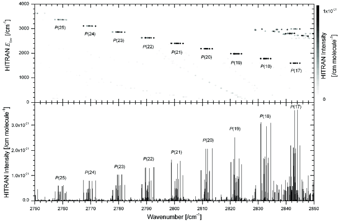
(a) Cluster splittings and $E_{low}$ values from HITRAN

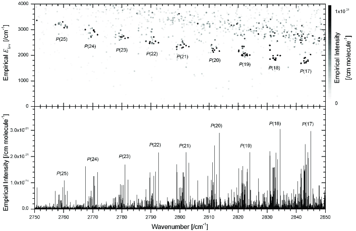
(b) Cluster splittings and empirical $E_{low}$ values

Figure 4: Cluster splitting of the $P$-branch lines of the $\nu_{3}$ mode of CH₄. Panel (a) contains the HITRAN $E_{low}$ values plotted with the scaled HITRAN lines at 1000^∘C and panel (b) contains the empirical $E_{low}$ values plotted with the calibrated lines at 1000^∘C. The grey scale of the $E_{low}$ value is taken from the intensity of the line at 1000^∘C.

It is worth noting that points below an $E_{low}$ of approximately 1000 cm^-1 are absent from Figure 3 due to the temperature gradient within the alumina tube. The CH₄ in the cooler ends of the tube absorbs the low-$J$ emission lines of the fundamental bands and accounts for the fact that only high-$J$ levels are seen in the branches of the $\nu_{3}$ mode as shown in Figures 3 and 4.

Self-absorption appears in our emission spectra as either complete absorption, resulting in a missing line, or as partial absorption which gives a distinctive double peak (Hargreaves et al., 2011). In order to provide more complete line lists we have added the missing lines from HITRAN to our line lists. We therefore incorporate HITRAN lines ($\pm$0.0025 cm^-1) with an intensity greater than that of a threshold value at each temperature. Our sensitivity decreases toward higher wavenumbers (regions A, C and D from Figure 1) and as a result the cut-off threshold is not a constant and changes over each region in order to match the sensitivity of the observations. The effect of adding HITRAN lines to our line lists is shown in Table 6 which lists the added HITRAN lines and the observed emission lines. In order to avoid double counting of lines, all lines in the emission line list within $\pm$0.0025 cm^-1 of a HITRAN line (with an intensity above the selection threshold) were deleted and replaced by the HITRAN lines.

Table 6: Line list summary

Temperature (∘C)	Observed Lines	Added HITRAN Lines	Total Lines
300	3,255	9,120	12,375
400	6,542	14,803	21,345
500	12,437	21,518	33,955
600	19,247	29,471	48,718
700	23,644	31,249	54,893
800	30,368	37,708	68,076
900	34,929	38,218	73,147
1000	37,706	38,559	76,265
1100	39,485	39,613	79,098
1200	28,532	30,419	58,951
1300	30,189	28,218	58,407
1400	19,788	17,067	36,855

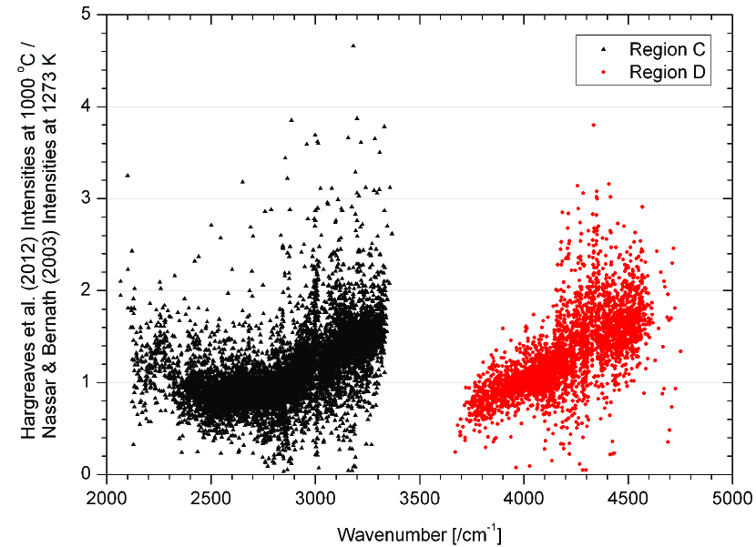
Figure 5: Comparison of line intensities at 1000^∘C with the values for corresponding lines (within $\pm$0.0025 cm^-1) recorded by Nassar & Bernath (2003) at 1273 K.

Comparisons made with Nassar & Bernath (2003) at 1000^∘C ($\pm$0.0025 cm^-1) suggest our intensities are accurate to within a factor of two (Figure 5). To estimate the error in the empirical $E_{low}$ values they were compared to those found in HITRAN for a number of lines which occur in both data sets. Table 7 shows that the percentage difference between the empirical $E_{low}$ calculation and HITRAN for the lines plotted in Figure 2 is less than 10 %. The examples shown are lines which appear in all spectra and as a result are the most reliable. These particular lines have also been removed from our final line lists because they coincide with HITRAN lines. As the number of points used to calculate the lower state energy decreases, the error increases. It is therefore difficult to quote an overall error for our $E_{low}$ values but we aim to represent the error by the inclusion of a quality factor within the line lists. ‘H’ signifies that the line position, intensity and lower state energy has been inserted from the HITRAN database. ‘1’ means that the lower state energy has been calculated from the intensities of a line that appears in 10 or more spectra. ‘2’ refers to any line which appears in 6 to 9 spectra and ‘3’ denotes that the lower state energy has been determined from 3 to 5 spectra. Finally, a ‘0’ indicates that the lower state energy could not be determined from the spectra available; in this case it means that the line occurs in less than 3 spectra in total. It should be noted that for region D a maximum quality factor of only ‘2’ is achievable. An extract of the hot CH₄ line list at 1000^∘C is displayed in Table 8, the complete line lists are available from the website of the Astrophysical Journal.

Table 7: Empirical lower state energy errors

Line	Wavenumber	Calculated $E_{low}$	HITRAN $E_{low}$	Difference
	(cm-1)	(cm-1)	(cm-1)	%
$\tilde{\nu}[1]$	1313.30	1364.00	1336.88	2.0
$\tilde{\nu}[2]$	3072.57	1590.79	1494.72	6.4
$\tilde{\nu}[3]$	1323.51	1644.41	1639.18	0.3
$\tilde{\nu}[4]$	1304.20	1879.95	1780.71	5.6
$\tilde{\nu}[5]$	1301.59	2036.83	1976.72	3.0

Table 8: Extract of the 1000^∘C hot CH₄ line list

Temperature	Wavenumber	Intensity	$E_{\textrm{low}}$	Quality
(∘C)	(cm-1)	(cm molecule-1)	(cm-1)	Factor
…	…	…	…	…
1000	1343.952393	4.21E-22	3.29E+03	1
1000	1343.962722	1.31E-23	1.82E+03	H
1000	1343.974972	1.98E-23	2.17E+03	H
1000	1343.980835	8.99E-23	3.08E+03	2
1000	1343.982910	8.99E-23	2.78E+03	1
1000	1343.992990	2.85E-23	1.93E+03	H
1000	1344.015503	3.96E-23	5.20E+03	3
1000	1344.033569	1.19E-22	3.18E+03	1
…	…	…	…	…

4 DISCUSSION

We have produced CH₄ line lists which can be used at temperatures from 300^∘C to 1400^∘C. The calibration of the wavenumber scale for each spectrum was done by making wavenumber comparisons of 20 lines to the HITRAN database and this gives an overall accuracy of better than 0.005 cm^-1. The wavenumber calibration is straightforward but intensity calibration is more difficult. Line intensities are notoriously hard to calibrate and our calibration was made by comparing as many lines as possible to the HITRAN database. Our overall line intensity accuracy is estimated to be approximately a factor of two. Intensity matches for lower wavenumbers (regions A and B) were good and allowed a consistent calibration function to be determined. Each region overlapped the neighbouring region with enough emission lines to place all regions on the same scale. For region D the intensity matches with HITRAN were effectively absent so a calibration factor could not be determined from this region alone. Since all regions are on the same scale, the calibration function was extrapolated into region D. In order to validate our extrapolation we were able to compare our 1000^∘C spectrum with the equivalent 1273 K spectrum from Nassar & Bernath (2003). The matches ($\pm$0.0025 cm^-1) can be seen in Figure 5 and show a clear intensity correlation to within a factor of two which gives confidence in the calibration applied. The slope is present because the Nassar & Bernath (2003) calibrations were performed using a single factor whereas the calibration used here is a parabolic function.

It is difficult to estimate an error for the empirical $E_{low}$ values presented here because self absorption causes inaccurate intensities resulting in inaccurate empirical $E_{low}$ values. This means comparisons can only be made between emission lines removed from the line lists and lines inserted from the HITRAN database. Comparison of the $E_{low}$ values of the five lines in Figure 2 can give a false impression of the accuracy, as in Table 7. A better estimate can be obtained by plotting the ratio of $E_{low}$ from HITRAN compared to the empirical $E_{low}$ values of the removed lines (Figure 6 at 1000^∘C). It clearly shows that the most common value of the HITRAN $E_{low}$ /empirical $E_{low}$ ratio is approximately one and that the majority of empirical $E_{low}$ values are accurate to within 20 %. It can be seen that the most accurate lines (with a quality factor of ‘1’) also display the smallest spread as opposed to the least accurate lines (quality factor of ‘3’). Figure 6 also shows why it was necessary to remove these lines because there is a tendency towards low ratios ($<1$) due to inaccurate line intensities caused by self absorption.

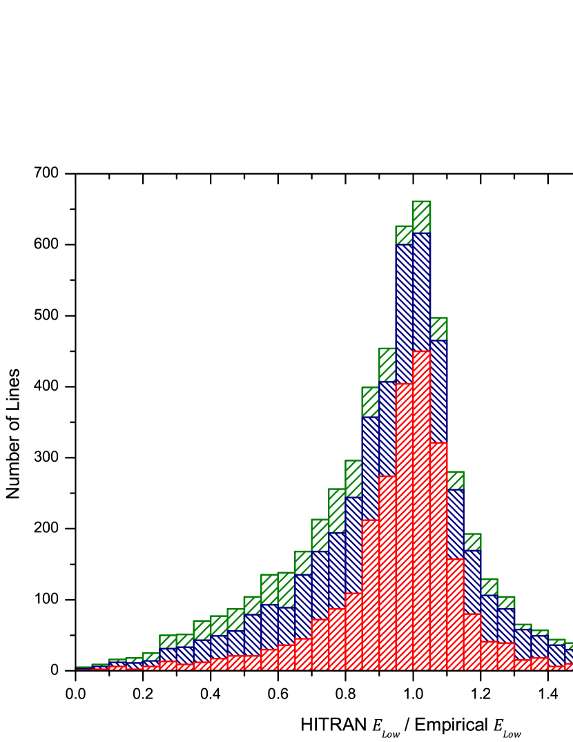
Figure 6: Histogram showing the ratios of the HITRAN $E_{low}$ values to the empirical $E_{low}$ values. The vertical bars of the histogram have been shaded to indicate the number of points with the quality factors (QF) 1, 2 and 3.

At high temperatures, thermal decomposition of methane is expected (Thiévin et al., 2008) and lower intensities are indeed observed for our high temperature spectra. The highest temperature spectra recorded in region D (1200^∘C and 1300^∘C) were contaminated by the absorption and emission of the products of thermal decomposition, namely C₂H₂ and C₂H₄. Attempts have been made to remove these species by using recent line lists (Moudens et al., 2011; Rothman et al., 2009); however, the emission features could not be completely removed. As this is the case, the hot CH₄ emission lines could not be distinguished from the products of thermal decomposition and the 1200^∘C and 1300^∘C files of region D have been excluded from our analysis.

Empirical $E_{low}$ values have been determined previously using a similar method by our group for the hot line lists of NH₃ (Hargreaves et al., 2011, 2012). It has also been used in the submillimeter regime (Fortman et al., 2010) and on ‘cold’ CH₄ in the infrared (Sciamma-O’Brien et al., 2009; Lyulin et al., 2010; Wang et al., 2012). Fortman et al. (2010) obtained $E_{low}$ values of an astrophysical ‘weed’ (ethyl cyanide) using numerous cool (-$40$ – $140^{\circ}$C) spectra. Sciamma-O’Brien et al. (2009), Lyulin et al. (2010) and Wang et al. (2012) have used a similar approach to study CH₄ based on a small number of room temperature and cold ($\sim$80 K) spectra. The method presented here uses a dozen ‘hot’ (300 – 1400^∘C) spectra which were recorded under conditions that are similar to those found in the atmospheres of brown dwarfs and hot-Jupiters. The use of a large number of spectra improves the accuracy of the $E_{low}$ values. However a single spectrum takes us many hours to record (including heating and cooling of the system) so it is impractical to record many additional spectra. Nevertheless, combining both hot and cold CH₄ line lists would help to complete the knowledge of CH₄ in the infrared.

Our method produces a relatively small number of lines with high line position accuracy. An alternative approach is to use ab initio calculations which provide significantly more lines but the line positions have much lower accuracy. The two methods are complementary and they can be combined to produce a merged line list. Zobov et al. (2011) have used the ab initio approach and were able to assign quantum numbers to some of our new NH₃ data; similar calculations are currently underway for CH₄.

The CH₄ line lists are available as electronic supplements via the website of the Astrophysical Journal (2013, ApJ, 774, 89, doi:10.1088/0004-637X/774/1/89) and spectra can also be provided upon request. The line lists should be used at the specified temperature; if a temperature is needed between those provided, we recommend scaling the lines using Equation 2. Only line lists from this erratum should be used.

5 CONCLUSION

Experimental line lists of hot CH₄ have been provided which contain calibrated wavenumbers (in cm^-1), calibrated intensities (in cm molecule^-1) and empirical lower state energies (in cm^-1). The line lists were based on 12 emission spectra recorded at 300 – 1400^∘C in 100^∘C intervals using a FT-IR spectrometer and cover the 960 – 5000 cm^-1 wavenumber range. This range contains the dyad, pentad and octad infrared regions of CH₄. The line lists can be used directly to model CH₄ in brown dwarfs and exoplanets. They also provide new experimental data for comparison with theoretical predictions.

References

- Albert et al. (2009) Albert, S., Bauerecker, S., Boudon, V., Brown, L. R., Champion, J. -P., Loëte, M., Nikitin, A., & Quack, M. 2009, J. Chem. Phys., 356, 131.
- Barman (2008) Barman, T. S. 2008, ApJ, 676, L61.
- Bernath (2005) Bernath, P. F. 2005, Spectra of Atoms and Molecules: Second Edition (Oxford: Oxford Univ. Press).
- Bernath (2009) Bernath, P. F. 2009, Int. Rev. Phys. Chem., 28, 681.
- Boudon et al. (2006) Boudon, V., Rey, M., & Loëte, M. 2006, J. Quant. Spec. Radiat. Transf., 98, 394.
- Borucki et al. (2012) Borucki, W. J., et al. 2012, ApJ, 745, 120.
- Burrows et al. (2001) Burrows, A., Hubbard, W. B., Lunine, J. I., & Liebert, J. 2001, Rev. Mod. Phys., 73, 719.
- Carleer (2001) Carleer, M. R. 2001, Proc. SPIE, 4168, 337.
- Campargue et al. (2012a) Campargue, A., Leshchishina, O., Wang, L., Mondelain, D., Kassi, S., & Nikitin, A. V. 2012a, J. Quant. Spec. Radiat. Transf., 113, 1855.
- Campargue et al. (2012b) Campargue, A., et al. 2012b, Icarus, 219, 110.
- Cassan et al. (2012) Cassan, A., et al. 2012, Nature, 481, 167.
- Cassam-Chenaï & Liévin (2012) Cassam-Chenaï, P. & Liévin, J. 2012, J. Chem. Phys., 136, 174309.
- Cassam-Chenaï (2003) Cassam-Chenaï, P. 2003, J. Quant. Spec. Radiat. Transf., 82, 251.
- Charbonneau et al. (2000) Charbonneau, D., Brown, T. M., Latham, D. W., & Mayor, M. 2000 ApJ, 529, L45.
- Charbonneau et al. (2002) Charbonneau, D., Brown, T. M., Noyes, R. W., & Gilliland, R. L. 2002, ApJ, 568, 377.
- Cushing et al. (2006) Cushing, M. C., at al. 2006, ApJ, 648, 614.
- Cushing et al. (2011) Cushing, M. C., et al. 2011, ApJ, 743, 50.
- Fortman et al. (2010) Fortman, S. M., Medvedev, I. R., Neese, C. F., & De Lucia, F. C. 2010, ApJ, 714, 476.
- Geballe et al. (2002) Geballe, T. R., et al. 2002, ApJ, 564, 466.
- Grillmair et al. (2008) Grillmair, C. J., Burrows, A., Charbonneau, D., Armus, L., Stauffer, J., Meadows, V., van Cleve, J., von Braun, K., & Levine, D. 2008, Nature, 456, 767.
- Hargreaves et al. (2010) Hargreaves, R. J., Hinkle, K. H., Bauschlicher, C. W., Wende, S., Seifahrt, A., & Bernath, P. F. 2010, AJ, 140, 919.
- Hargreaves et al. (2011) Hargreaves, R. J., Li, G., & Bernath, P. F. 2011, ApJ, 735, 111.
- Hargreaves et al. (2012) Hargreaves, R. J., Li, G., & Bernath, P. F. 2012, J. Quant. Spec. Radiat. Transf., 113, 670.
- Hauschildt et al. (2009) Hauschildt, P. H., Warmbier, R., Schneider, R., & Barman, T. 2009, A&A, 504, 225.
- Herzberg (1991) Herzberg, G. 1991, Molecular Spectra and Molecular Structure: VolumeIII - Electronic Spectra and Electronic Structure of Polyatomic Molecules (Malabar: Krieger Publishing Company).
- IPCC (2007) Intergovernmental Panel on Climate Change 2007, Fourth Assessment Report: Climate Change 2007: The AR4 Synthesis Report (Geneva: IPCC).
- Karkoschka (1994) Karkoschka, E. 1994, Icarus, 111, 174.
- Kirkpatrick (2005) Kirkpatrick, J.D. 2005, ARA&A, 43, 195.
- Kirkpatrick et al. (2011) Kirkpatrick, J. D., et al. 2011, ApJS, 197, 19.
- Laraia et al. (2011) Laraia, A. L., Gamache, R. R., Lamouroux, J., Gordon, I. E., & Rothman, L. S. 2011, Icarus 215, 391.
- Leggett et al. (2001) Leggett, S. K., Allard, F., Geballe, T. R., Hauschildt, P. H., & Schweitzer, A. 2001, ApJ, 548, 908.
- Lyulin et al. (2010) Lyulin, O. M., Kassi, S., Sung, K., Brown, L. R., & Campargue, A. 2010, J. Mol. Spec., 261, 91.
- Mayor & Queloz (1995) Mayor, M., & Queloz, D. 1995, Nature, 378,355.
- Mondelain et al. (2011) Mondelain, D., Kassi, S., Wang, L., & Campargue, A. 2011, Phys. Chem. Chem. Phys., 13, 7985.
- Moudens et al. (2011) Moudens, A., Georges, R., Benidar, A., Amyay, B., Herman, M., Fayt, A., & Plez, B. 2011, J. Quant. Spec. Radiat. Transf., 112, 540.
- Mumma et al. (2009) Mumma, M. J., Villanueva, G. L., Novak, R. E., Hewagama, T., Bonev, B. P., DiSanti, M. A., Mandell, A. M., & Smith, M. D. 2009, Science, 323, 1041.
- Nassar & Bernath (2003) Nassar, R., & Bernath, P. 2003, J. Quant. Spec. Radiat. Transf., 82, 279.
- Niemann et al. (2005) Niemann, H. B., et al. 2005, Nature, 438, 779.
- Nikitin et al. (2011) Nikitin, A. V., Rey, M., & Tyuterev, V. G. 2011, Chem. Phys. Lett., 501, 179.
- Perrin & Soufiani (2007) Perrin, M. -Y., & Soufiani, A. 2007, J. Quant. Spec. Radiat. Transf., 103, 3.
- Rothman et al. (2009) Rothman, L. S., et al. 2009, J. Quant. Spec. Radiat. Transf., 110, 533.
- Seager & Deming (2010) Seager, S., & Deming, D. 2010, ARA&A, 48, 631.
- Schwenke & Partridge (2001) Schwenke, D. W., & Partridge, H., 2001, Spectrochimica Acta A, 57, 887.
- Schwenke (2002) Schwenke, D. W. 2002, Spectrochimica Acta A, 58, 849.
- Sciamma-O’Brien et al. (2009) Sciamma-O’Brien, E., Kassi, S., Gao, B., & Campargue, A. 2009, J. Quant. Spec. Radiat. Transf., 110, 951.
- Stofan et al. (2007) Stofan, E. R., et al. 2007, Nature, 445, 61.
- Swain et al. (2008) Swain, M. R., Vasisht, G., & Tinetti, G. 2008, Nature, 452, 329.
- Swain et al. (2009a) Swain, M. R., et al. 2009a, ApJ, 704, 1616.
- Swain et al. (2009b) Swain, M. R., Vasisht, G., Tinetti, G., Bouwman, J., Chen, P., Yung, Y., Deming, D., & Deroo, P. 2009b, ApJ, 690, L114.
- Thiévin et al. (2008) Thiévin, J., Georges, R., Carles, S., Benidar, A., Rowe, B., & Champion, J. -P. 2008, J. Quant. Spec. Radiat. Transf., 109, 2027.
- Tinetti et al. (2010) Tinetti, G., Deroo, P., Swain, M. R., Griffith, C. A., Vasisht, G., Brown, L. R., Burke, C., & McCullough, P. 2010, ApJ, 712, L139.
- Wang et al. (2012) Wang, L., Mondelain, D., Kassi, S., & Campargue, A. 2012, J. Quant. Spec. Radiat. Transf., 113, 47.
- Wang et al. (2011) Wang, L., Kassi, S., Liu, A. W., Hu, S. M., & Campargue, A. 2011, J. Quant. Spec. Radiat. Transf., 112, 937.
- Wang & Carrington (2004) Wang, X.-G., & Carrington Jr., T. 2004, J. Chem. Phys., 121, 2937.
- Wang & Sibert (2002) Wang, X.-G., & Sibert III, E. L. 2002, Spectrochimica Acta A, 58, 863.
- Wenger et al. (2008) Wenger, Ch., Champion, J. P., & Boudon, V. 2008, J. Quant. Spec. Radiat. Transf., 109, 2976.
- Warmbier et al. (2009) Warmbier, R., Schneider, R., Sharma, A. R., Braams, B. J., Bowman, J. M., & Hauschildt, P. H. 2009, A&A, 495, 655.
- Zobov et al. (2011) Zobov, N. F., Shirin, S. V., Ovsyannikov, R. I., Polyansky, O. L., Yurchenko, S. N., Barber, R. J., et al. 2011, J. Mol. Spectrosc., 269, 104.