RR Lyrae variables: visual and infrared luminosities, intrinsic colours, and kinematics

Abstract

We use UCAC4 proper motions and WISE $W1$-band apparent magnitudes intensity-mean for almost 400 field RR Lyrae variables to determine the parameters of the velocity distribution of Galactic RR Lyrae population and constrain the zero points of the metallicity-$<M_{V}>$ relation and those of the period-metallicity-$<M_{K_{s}}>$-band and period-metallicity-$<M_{W1}>$-band luminosity relations via statistical parallax. We find the mean velocities of the halo- and thick-disc RR Lyrae populations in the solar neighbourhood to be ($U_{0}(Halo),V_{0}(Halo),W_{0}(Halo)$) = $(-7\pm 9,-214\pm 10,-10\pm 6)$ km s^-1 and ($U_{0}(Disc),V_{0}(Disc),W_{0}(Disc)$) = $(-13\pm 7,-37\pm 6,-17\pm 4)$ km s^-1, respectively, and the corresponding components of the velocity-dispersion ellipsoids, ($\sigma V_{R}(Halo),\sigma V_{\phi}(Halo),\sigma V_{\theta}(Halo)$) = $(153\pm 9,101\pm 6,96\pm 5)$ km s^-1 and ($\sigma V_{R}(Disc),\sigma V_{\phi}(Disc),\sigma V_{\theta}(Disc)$) = $(46\pm 7,37\pm 5,27\pm 4)$ km s^-1, respectively. The fraction of thick-disc stars is estimated at 0.22 $\pm$ 0.03. The corrected IR period-metallicity-luminosity relations are $<M_{K_{s}}>$ = -0.769 +0.088 $\cdot$ [Fe/H]- 2.33 $\cdot\mathop{\rm log}P_{F}$ and $<M_{W1}>$ = -0.825 + 0.088$\cdot$ [Fe/H] -2.33 $\cdot\mathop{\rm log}P_{F}$, and the optical metallicity-luminosity relation, [Fe/H]-$<M_{V}>$, is $<M_{V}>$ = +1.094 + 0.232$\cdot$ [Fe/H], with a standard error of $\pm$ 0.089, implying an LMC distance modulus of 18.32 $\pm$ 0.09, a solar Galactocentric distance of 7.73 $\pm$ 0.36 kpc, and the M31 and M33 distance moduli of $DM_{M31}$ = 24.24 $\pm$ 0.09 ($D$ = 705 $\pm$ 30 kpc) and $DM_{M33}$ = 24.36 $\pm$ 0.09 ($D$ = 745 $\pm$ 31 kpc), respectively. Extragalactic distances calibrated with our RR Lyrae star luminosity scale imply a Hubble constant of $\sim$80 km/s/Mpc. Our results suggest marginal prograde rotation for the population of halo RR Lyraes in the Milky Way.

1 Introduction

RR Lyrae variables are A-F type giants undergoing core helium burning, which pulsate with periods 0.2-1.2 d and have masses and luminosities of $M\sim 0.7M_{\odot}$ and $L=40-50L_{\odot}$, respectively. They are easy to identify by their periods and characteristic light-curve shapes and, like other pulsating stars, obey a period-metallicity-luminosity relation, which in the case of the $V$- and $K$- bands appears to degenerate into the metallicity-luminosity and period-luminosity relations, respectively (Catelan et al., 2004), both characterised by a very low intrinsic scatter of $\leq 0.06-0.09^{m}$ (Wagner-Kaiser & Sarajedini, 2013; Frolov & Samus, 1998). Because of the large ages ($>$ 10 Gyr) of RR Lyrae variables these stars occur in systems with old populations (globular clusters, elliptical galaxies, halos and thick discs of spiral galaxies, irregular galaxies) and can therefore serve as distance indicators, as well as kinematic and metallicity tracers. Although their factor of $\sim$ 100 lower luminosities have long left RR Lyraes somewhat overshadowed by Cepheids as extragalactic distance indicators, recent progress in extragalactic stellar photometry has made them an efficient tool for mapping the Local Group, and one of the most important contributors to the first rung of the cosmic distance scale (Cacciari, 2013).

However, for RR Lyraes to be properly usable to this end, the parameters of the period-metallicity-luminosity relations in various bands have to be established with adequate precision. The problem is that although a consensus seems to have emerged concerning the slopes of the corresponding relations in various photometric bands, this still is far from true for the respective zero-points: they, like 17 years ago, ”continue to defy a consensus” (Layden et al., 1996) with estimates reported by different authors spanning a $\sim$ 0.3-0.5^m wide interval.

Six decades ago, Pavlovskaya (1953) was the first to apply the statistical-parallax technique to estimate the mean absolute magnitude of RR Lyrae stars. Since then, the method, continuously refined, has been used extensively by many authors (Pavlovskaya, 1953; Rigal, 1958; van Herk, 1965; Clube & Dawe, 1980; Hawley et al., 1986; Strugnell, 1986; Layden et al., 1996; Popowski & Gould, 1998a, b; Gould & Popowski, 1998; Fernley et al., 1998a; Tsujimoto, 1998; Luri et al., 1998; Dambis & Rastorguev, 2001; Dambis, 2003; Dambis & Vozyakova, 2004; Rastorguev, Dambis & Zabolotskikh, 2005; Dambis, 2009; Kollmeier et al., 2012) with ever increasing samples of RR Lyrae stars. The current, maximum-likelihood version of the technique was first proposed by Murray (1983), and its practical application dates back to Strugnell (1986) and Hawley et al. (1986). Layden et al. (1996) were the first to take into account the kinematic inhomogeneity of the local RR Lyrae population by a priori attributing each star either to the halo or thick-disc subsample based on metallicity and velocity data. Luri et al. (1996) generalised the method to explicitly incorporate the eventual multicomponent structure of the population studied, and Luri et al. (1998) applied the generalised technique to Galactic RR Lyrae type stars. One of the solutions in our previous study (Dambis, 2009) also took into account the bimodal nature of the velocity distribution without a priori partitioning the sample into two groups.

Time has now come for yet another statistical-parallax based study of RR Lyrae type stars to be performed for two main reasons. First, impressive progress has been achieved in the photometry of RR Lyrae variables, with good light curves obtained for many stars. These include (a) extensive optical data acquired both within the framework of ASAS survey (Pojmanski, 2002) and as a result of our dedicated program of photometric observations of RR Lyrae stars (Berdnikov et al., 2011a, b, 2012), and (b) infrared light curves acquired within the framework of WISE all-sky photometric survey (Wright et al., 2010) supplemented by single-phase 2MASS $JHK_{s}$-band measurements (Cutri et al., 2003), which, given precise light elements, can be converted to the corresponding intensity-mean magnitudes (Feast et al., 2008). As a result, bona fide multicolour intensity-mean magnitudes have for the first time become available simultaneously for the bulk of $\sim$ 400 Galactic field RR Lyrae type variables with known radial velocities and metallicities, allowing the interstellar extinction to be accurately determined for all these objects. Second, the release of the final, fourth version of The US Naval Observatory CCD Astrograph Catalogue (UCAC4)(Zacharias et al., 2013), which provides very accurate proper motions for most of the stars down to an $R$-band limiting magnitude of about 16^m, allows the statistical-parallax study to be based on a single source of proper motions throughout the entire sky.

The primary aim of this paper is to refine the infrared and visual photometric distance scales of RR Lyrae variables by further constraining the zero points of the $V$-, $K_{s}$-, and WISE $W1$-band period-metallicity-colour relations for these stars via the method of statistical parallax, and use them to estimate the distances to a number of Local group galaxies. As a by product, we calibrate the $(V-K_{s})_{0}$ and $(V-W1)_{0}$ intrinsic colours of these stars and determine the kinematical parameters of the local RR Lyrae star population.

Section 2 describes the observational data that we use for our statistical-parallax analysis. In Section 3 we analyze the interstellar extinction toward our sample stars and derive the intrinsic-colour relations for RR Lyrae type stars in terms of fundamental period and metallicity. Section 4 is devoted to the initial (provisional) distances to our sample RR Lyraes to be adjusted. In Section 5 we say a few words about the statistical-parallax method employed and the (kinematical and distance-scale) parameters to be determined. In Section 6 we present the results of our analysis. In Sections 7, 8, and 9 we discuss the implications of our results for the cosmic distance scale, rotation of RR Lyrae populations, and cosmology, respectively. The final section summarizes the conclusions.

2 OBSERVATIONAL DATA

First, we tried to collect the most complete possible sample of Galactic field RR Lyrae type variables with measured radial velocities and metallicities. The sample we use in this paper is based mostly on that employed in our previous statistical-parallax analysis of RR Lyrae variables (Dambis, 2009), which, in turn, is based on the list of Galactic RR Lyraes from the revised catalogue of 2106 Galactic stars selected without kinematic bias and with available radial velocities, distance estimates, and metal abundances in the range -4.0$\leq$[Fe/H]$\leq$0.0 compiled by Beers et al. (2000). This list includes a total of 388 Galactic RR Lyrae stars, which we supplement with the data for 14 additional RR Lyrae type variables from recent papers. Thus our final sample contains 402 RR Lyrae type stars.

2.1 Periods and pulsation modes

Like in our previous study (Dambis, 2009), we adopt the periods of the RR Lyrae type stars of our sample from the ASAS catalogue (Pojmanski, 2002), Maintz (2005), or the General Catalogue of Variable Stars (Samus et al., 2013). The latter was our source of pulsation modes. We use the formula $P_{F}$ = log $P$ + 0.127 (Frolov & Samus, 1998) to fundamentalise the periods of RRc type variables (first-overtone pulsators).

2.2 Apparent intensity-mean magnitudes

2.2.1 $V$-band data

Layden et al. (1996) characterised the available $V$-band photometry for Galactic field RR Lyrae variables as a ”surprisingly heterogeneous data set”, and this is still true after 17 years, although extensive optical data has been acquired since then as a result of ASAS survey (Pojmanski, 2002) and our own dedicated program (Berdnikov et al., 2011a, b, 2012). In this paper, we derive the intensity-mean Johnson $V$-band magnitudes $<V>$ based on nine sufficiently large overlapping sets of photoelectric and CCD observations (Bookmeyer et al. (1977) (1), ASAS (Pojmanski, 2002) (2), HIPPARCOS $H_{p}$-band photometry (ESA, 1997) (3), Lub (1977); van Genderen et al. (1980) (4), Clube & Dawe (1980) (5), our own data Berdnikov et al. (2011a, b, 2012) (6), Schmidt (1991); Schmidt et al. (1995); Schmidt & Seth (1996) (7), Layden (1994, 1997); Day et al. (2002) (8), Kinman (1961, 1982, 2002); Kinman & Brown (2010) (9)). In the case of the data of Bookmeyer et al. (1977) and Clube & Dawe (1980) we computed the initial intensity means $<V>$ using Eq. (1) from Layden (1994). We adopted the initial intensity-mean $<V>$ magnitudes based on HIPPARCOS $H_{p}$-band photometry from Fernley et al. (1998a) or computed them in accordance with the procedure described by the above authors for stars lacking in their paper. In the case of observations made in the five-colour Walraven system we adopted the Johnson magnitude means $<V>_{m}$ listed by Lub (1977) and computed the corresponding magnitude means based on the data reported by van Genderen et al. (1980). In the case of ASAS data we determined the intensity means $<V>$ from the light-curve fits defined by the Fourier coefficients reported by Szczygieł et al. (2009) or computed them directly from ASAS data for the stars lacking in the list of Szczygieł et al. (2009). We thus have a set of mean magnitudes $<V_{ik}>$ for our stars, where $i$ and $j$ are the number of the dataset and the number of the star, respectively. As mentioned above, $<V_{ik}>$ is the initial intensity-mean magnitude estimate, except for the case of dataset $i$=4 (Lub, 1977; van Genderen et al., 1980), which consists of magnitude means. We then determine the homogeneous intensity-mean $<V_{k}>_{final}$ magnitudes for our stars and the correcting offsets $\Delta V_{i}$ by solving the following set of linear equations:

$$<V_{k}>_{final}-\Delta V_{i}=<V_{ik}>$$ (1)

We adopt the dataset of Bookmeyer et al. (1977) as our standard system and set $\Delta V_{1}$ = 0 by definition. We collected a total of 905 mean magnitude estimates for 384 stars and hence have 905 equations for 384+8=392 unknowns. The resulting offsets $\Delta V_{i}$ are listed in column 4 of Table 1. Other columns list the number of the dataset (column 1), the references to the original data (column 2), the number of stars in the dataset (column 3), and remarks (column 5). The standard errors of the homogenised intensity-mean magnitudes $<V_{k}>_{final}$ range from $\sim$ 0.015^m to $\sim$ 0.035^m. The offsets can be seen to be generally small, and only in three cases do they appreciably exceed 0.01^m in absolute value: these correspond to datasets (4) (Lub, 1977; van Genderen et al., 1980), (5) (Clube & Dawe, 1980), and (7)(Schmidt, 1991; Schmidt et al., 1995; Schmidt & Seth, 1996). To reveal eventual metallicity-dependent systematics, we computed the intensity-mean magnitude differences $<V_{ik}>-<V_{2,k}>$ between each dataset and the largest dataset (2) (ASAS) and fitted them to a linear relation of the form

$$<V_{ik}>-<V_{2,k}>=p_{i}+q_{i}\cdot[Fe/H].$$ (2)

We found, as expected, the resulting metallicity slopes $q_{i}$ not to differ significantly from zero and range from -0.002 $\pm$0.023 to +0.020 $\pm$ 0.046 for all datasets except no. 8 (Layden, 1994, 1997; Day et al., 2002):

$$<V_{8}>-<V_{ASAS}>=$$

$$+0.104~{}\pm~{}0.045+(0.063~{}\pm~{}0.031)\cdot[Fe/H].$$ (3)

However, even in this case the slope barely exceeds 2$\sigma$ and is actually due to three clear outliers at the high-metallicity end (see Fig. 1). Note that two of these stars — UY Aps ($b=-11.39$) and V494 Sco ($b=-0.49$) — are located in crowded fields close to the Galactic equator, where ASAS performance is degraded because of the large pixel size ($\sim~{}15~{}arcsec^{2}$). We therefore homogenize $V$-intensity magnitudes without introducing any metallicity dependent terms.

Table 1: Sources of intensity-mean $V$-band magnitudes (based on photoelectric and CCD photometry)

Dataset	References	Number	$\Delta V_{i}$	Remark
no. (i)		of stars
1	Bookmeyer et al. (1977)	142	0.000 $\pm$ 0.000
2	ASAS (Pojmanski, 2002)	234	-0.001 $\pm$ 0.004
3	HIPPARCOS (ESA, 1997; Fernley et al., 1998a)	148	+0.009 $\pm$ 0.004	A
4	Lub (1977); van Genderen et al. (1980)	83	+0.054 $\pm$ 0.005	B
5	Clube & Dawe (1980)	59	-0.040 $\pm$ 0.006
6	Berdnikov et al. (2011a, b, 2012)	120	-0.005 $\pm$ 0.005
7	Schmidt (1991); Schmidt et al. (1995)	57	+0.018 $\pm$ 0.007
	Schmidt & Seth (1996)
8	Layden (1994, 1997); Day et al. (2002)	23	+0.013 $\pm$ 0.010
9	Kinman (1961, 1982, 2002)	28	+0.014 $\pm$ 0.013
	Kinman & Brown (2010)
Remarks: A.	Johnson’s $V$-band intensity-mean magnitudes
	converted from HIPPARCOS $<Hp>$ magnitudes
	as described by Fernley et al. (1998a)
B.	Based on magnitude means in the Walraven
	five-colour VBLUW system. Johnson’s $V_{J}$-band
	magnitude means computed by the formula
	$V_{J}$ = 6.874m - 2.5 ${V+0.065(V-B)}$ (Pel, 1976)

Figure 2 shows the distribution of the stars by the number of mean magnitude estimates and Fig. 3, the distribution of the standard errors of the final $V$-band intensity means, $\sigma<V_{k}>_{final}$.

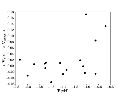
Figure 1: Intensity-mean magnitude difference between dataset (8) (Layden, 1994, 1997; Day et al., 2002) and ASAS as a function of metallicity.

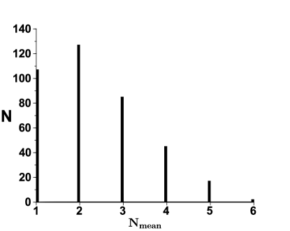
Figure 2: Histogram of the number of $<V>$ sources per star.

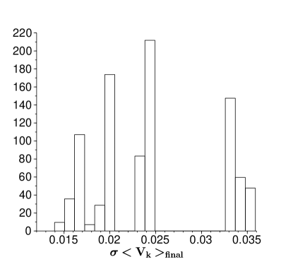
Figure 3: Histogram of standard errors of the final intensity-mean $<V>$-band magnitudes.

2.2.2 $K_{s}$-band data

As we already pointed out (Dambis, 2009), the 2MASS project, which mapped the entire sky in three near-infrared bands – $J$, $H$, and $K_{s}$, provides homogeneous near-infrared photometry for almost all Galactic RR Lyrae type variables with known metallicities and radial velocities. Another important advantage of 2MASS data over available optical photometry is its highly reduced sensitivity to interstellar extinction, which is one order of magnitude smaller in the $K_{s}$ band than in the $V$ band (Yuan et al., 2013). We adopt the intensity-mean $K_{s}$-band magnitudes for most of the stars of our sample from Dambis (2009). These are single-epoch 2MASS magnitudes phase corrected in accordance with the procedure described by Feast et al. (2008) (including the data adopted from Kinman et al. (2007) for 13 stars), which are accurate to within $\sim 0.03^{m}$ (summed quadratically with error of the observed 2MASS $K_{s}$ magnitude), or just raw 2MASS magnitudes with no phase correction applied (in the case of no or too outdated ephemeris) for 32 stars. For the additional 12 stars we determine the intensity-mean $K_{s}$-band magnitudes by phase correcting their 2MASS $K_{s}$-band magnitudes using the same procedure described by Feast et al. (2008) (for five stars) or adopting the phase-corrected 2MASS $K_{s}$ magnitude from Kinman et al. (2007) (one star) and Kinman et al. (2012) (six stars). We have collected intensity-mean $K_{s}$-band estimates for all 403 RR Lyrae type variables of our sample.

2.2.3 WISE $W1$-band data

The WISE All-Sky Data Release, which was made public last year (Cutri et al., 2012) and which mapped the entire sky in four mid-infrared bands W1, W2, W3, and W4 with the effective wavelengths of 3.368, 4.618, 12.082 and 22.194 $\mu$m, respectively (Wright et al., 2010), is even better suited for building the distance scale of RR Lyrae type variables. Its chief advantages over 2MASS are the true homogeneity (measurements performed over the entire sky with a single instrument operating beyond the earth atmosphere), a factor of $\sim$ 1.7 smaller sensitivity to interstellar extinction (Yuan et al., 2013), and good phase coverage for short-period variables with at least a dozen well-distributed measurements available for all stars and over a thousand measurements made for stars near the ecliptic poles. We used the WISE single-exposure database to compute the intensity-mean average W1-band magnitudes, $<W1>$, for a total of 398 stars of our sample. Figure 4 shows the WISE W1 light curves for a TT Lyn, a typical RR Lyrae variable from our list, and Fig. 5 shows the WISE W1 light curve of VW Dor, which is located close to the South Ecliptic Pole at the ecliptic latitude of -89.129^∘.

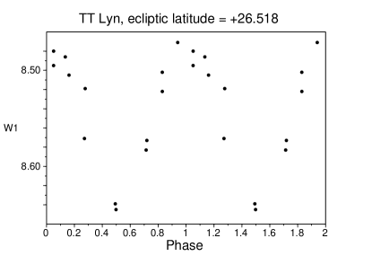
Figure 4: WISE W1 light curve of TT Lyn.

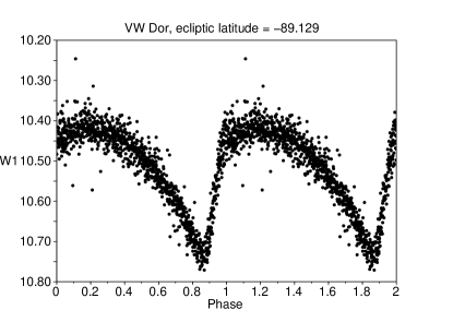
Figure 5: WISE W1 light curve of VW Dor.

2.3 Metallicities

For most of the stars of our sample we use the homogenised metallicities on the Zinn & West (1984) scale adopted from the compilation of Dambis (2009), which, in turn, is mostly based on the catalogue of Beers et al. (2000). All these metallicities are based on spectroscopic measurements. Our sources of metallicities for the additional stars lacking in the sample of Dambis (2009) were Fernley & Barnes (1997) (BH Aur, V363 Cas, and EZ Cep, reduced to the Zinn and West scale via formula (46) in Dambis (2009)), Layden (1994) (ET Hya, , already on the Zinn and West scale), Pier et al. (2003) (RW Lyn, reduced to the Zinn and West scale via formula (46) in Dambis (2009)), Kinman et al. (2007) (MO Com, reduced to the Zinn and West scale via formula (46) in Dambis (2009)), Kinemuchi et al. (2006) (EN Lyn, photometric metallicity on the Zinn and West scale), Kemper (1982) (BK UMa and BN UMa, delta S values reduced to [Fe/H] on the Zinn and West scale). We computed the photometric metallicities of CH Aql (from ASAS light-curve parameters) and DQ Lyn (from NSVS light-curve parameters) using formula (14) from Kinemuchi et al. (2006) and formula (3) from Morgan et al. (2007), respectively. We thus have collected homogenised metallicities for a total of 402 stars of our sample (no metallicity could be determined for CK UMa). Figure 6 shows the distribution of metallicities for stars of our sample.

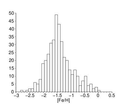
Figure 6: Distribution of metallicities of sample stars.

2.4 Radial velocities

We adopted the mean radial velocities, $V_{R}$, and their standard errors, $\sigma V_{R}$, for most of the stars from Dambis (2009), and the corresponding quantities for the additional stars, from Fernley & Barnes (1997) (BH Aur, V363 Cas, and EZ Cep), Jeffery et al. (2007) (CH Aql and BK UMa), Pier et al. (2003) (RW Lyn), Kinman et al. (2007) (MO Com), Kinman & Brown (2010) (DQ Lyn, EN Lyn, BN UMa, and CK UMa). We also updated the $\gamma$ velocities for seven stars (WY Ant, XZ Aps, BS Aps, Z Mic, RV Oct, V1645 Sgr, and AS Vir) based on the data reported by For et al. (2011). We collected the mean radial velocity estimates for all 403 stars of our sample. Figure 7 shows the distribution of radial-velocity errors for stars of our sample.

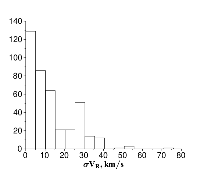
Figure 7: Distribution of radial-velocity errors of sample stars.

2.5 Proper motions

We adopt the fourth United States Naval Observatory (USNO) CCD Astrograph Catalogue, UCAC4, (Zacharias et al., 2013), which ”is complete from the brightest stars to about magnitude R = 16”, as our only source of absolute proper motions, which are available for 393 of the 403 stars of our list. Figure 8 shows the distribution of proper-motion errors in right ascension (the top panel) and declination (the bottom panel).

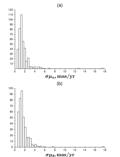
Figure 8: Distribution of proper-motion errors of sample stars in right ascension (a) and declination (b).

3 Interstellar extinction, period-metallicity-luminosity relations, and intrinsic colour calibrations

We now estimate the amount of interstellar extinction toward stars of our sample. The most straightforward way is to use a 2D extinction map and assign to each star the ”extinction at infinity”. This approach should work well for most of the stars except those located close to the Galactic plane. We consider it better to compute extinction in terms of the 3D extinction model by Drimmel et al. (2003). To do this, we need to approximately estimate the distances to our stars (we show below that choosing another, even significantly different published relation, has no effect on the colour calibrations and extinction estimates obtained in this section). We begin by estimating the absolute $K_{s}$-band magnitudes of our sample stars by adopting (provisionally) the following period-luminosity relation derived by Jones et al. (1992) based on the results obtained using the Baade-Wesselink method:

$$<M_{K(Jones)}>=-2.33\cdot\mathop{\rm log}P_{F}-0.88,$$ (4)

where $K$-band magnitudes are on the CIT system. Given the negligible and statistically insignificant coefficient of the colour term in the transformation equation (http://www.astro.caltech.edu/ jmc/2mass/v3/transformations/)

$$(K_{s})_{2MASS}=K_{CIT}+$$

$$(-0.019\pm 0.004)+(0.001\pm 0.005)(J-K)_{CIT}$$ (5)

and the fact that average $(J-K)$ colour indices of RR Lyrae type variables always lie inside the interval from 0.00^m to 0.50^m, period-$K_{CIT}$-band luminosity relation given by equation (4) transforms into the following period-$K_{s}$-band luminosity relation

$$<M_{K_{s}}>=-2.33\cdot\mathop{\rm log}P_{F}-0.90,$$ (6)

which we use to compute the absolute $K_{s}$-band magnitudes of our stars. We then use the 3D extinction model by Drimmel et al. (2003) to determine the amount of interstellar extinction toward each star via the following iterative procedure. We initially set the total $K_{s}$ band extinction equal to zero, $A_{K_{s}}$=0, and compute the distance (in kpc) by the following formula:

$$d=10^{0.2\cdot(<K_{s}>-A_{K_{s}}-M_{K_{s}})-2}.$$ (7)

We use this distance estimate and the star’s coordinates to compute the refined estimate of the amount of interstellar extinction, $A_{V}$, in terms of the model of Drimmel et al. (2003), transform it into $E(B-V)$ = $A_{V}/R_{V}$ ($R_{V}$ = 3.1 (Yuan et al., 2013)), compute $A_{K_{s}}$ = $R_{K}\cdot E(B-V)$ ($R_{K_{s}}$ = $A_{K_{s}}/E(B-V)$ = 0.306 (Yuan et al., 2013)), and refine the distance estimate via formula (7). We repeat this procedure until both $d$ and $A_{K_{s}}$ (and, naturally, $E(B-V)$, and $A_{V}$) converge.

A question naturally arises to which extent are our reddening estimates dependent on the adopted provisional distances to RR Lyrae type stars. To assess the effect of a different set of input distance estimates, we repeated the above procedure using two other popular period-metallicity-$<M_{K}>$ relations, which, compared to PL relation (6), yield brighter absolute magnitudes practically for all our stars, on the average by $\sim$ 0.35^m, translating into a factor of $\sim$ 1.17 longer distances. The one was derived theoretically by Bono et al. (2003):

$$<M_{K_{s}}>=-2.101\cdot\mathop{\rm log}P_{F}+0.231(\pm~{}0.012)\cdot[Fe/H]$$

$$-0.770(\pm~{}0.044),$$ (8)

and the other is an empirical one derived by Sollima et al. (2008) based on observational data for globular-cluster RR Lyrae variables:

$$<M_{K_{s}}>=-2.38(\pm~{}0.04)\cdot\mathop{\rm log}P_{F}+0.09(\pm~{}0.14)\cdot[Fe/H]$$

$$-1.07(\pm~{}0.11),$$ (9)

We found the distances based on the period-metallicity-$<M_{K}>$ relation of Bono et al. (2003) to yield $A_{V}$ values that differ by +0.0023$\pm$0.0004 with a scatter of 0.009 from those computed with distances based on relation (6). The corresponding difference for the calibration of Sollima et al. (2008) is +0.0031$\pm$0.0006 with a scatter of 0.011. The differences become truly negligible for the subsample of stars with $|b|~{}>~{}25^{\circ}$, on which our final colour calibrations are actually based (see below): +0.0002$\pm$0.0001 with a scatter of 0.0016 for both the relation of Bono et al. (2003) and that of Sollima et al. (2008). We can therefore safely assume that all the colour calibrations derived below do not depend on the provisional input distances used to estimate the interstellar extinction toward the calibrating RR Lyrae stars of our sample. Hence the final colour calibrations remain unchanged and so are the extinction values for low-latitude stars that are based on them. We point out that the provisional distances computed in this section serve the sole purpose of estimating the interstellar extinction and are not used below for any other end.

We now use the resulting $A_{V}$, $A_{K_{s}}$, and $A_{W1}=R_{W1}\cdot E(B-V)$ ($R_{W1}$ = $A_{W1}/E(B-V)$ = 0.18 (Yuan et al., 2013)) values to deredden the observed intensity-mean $<V>$, $<K_{s}>$, and $<W1>$ magnitudes:

$$<V>_{0}=<V>-A_{V},$$ (10)

$$<K_{s}>_{0}=<K_{s}>-A_{K_{s}},$$ (11)

$$<W1>_{0}=<W1>-A_{W1},$$ (12)

and the intrinsic colours:

$$(<V>-<K_{s}>)_{0}=<V>-<K_{s}>-(A_{V}-A_{K_{s}}),$$ (13)

$$(<K_{s}>-<W1>)_{0}=<K_{s}>-<W1>-(A_{K_{s}}-A_{W1}),$$ (14)

$$(<V>-<W1>)_{0}=<V>-<W1>-(A_{V}-A_{W1}).$$ (15)

We now calibrate the $(<V>-<K_{s}>)_{0}$ intrinsic colour index in terms of [Fe/H] and log $P_{F}$. We proceed based on the following two established facts. First, the absolute V-band magnitude of RR Lyrae variables depends on metallicity [Fe/H] and, for a given metallicity is independent of period (Catelan et al., 2004):

$$<M_{V}>=a_{v}+b_{v}\cdot[Fe/H],$$ (16)

where the most recent reliable direct empirical estimates of the slope $b_{v}$ are $b_{v}$ = 0.214 $\pm$ 0.047 (Gratton et al., 2004) and $b_{v}$ = 0.25 $\pm$ 0.02 (Federici et al., 2012). These estimates are based on the sole geometric assumption that the stars in question are in both cases at the same distance from us. Hereafter we adopt the simple (unweighted) average of the two:

$$<M_{V}>=a_{v}+0.232(\pm~{}0.020)\cdot[Fe/H],$$ (17)

We prefer to rely on the above estimates rather than on those based on Baade-Wesselink analyses (Cacciari et al., 1992; Skillen et al, 1993; Fernley et al., 1998b), which depend on more input assumptions and are therefore not enough ”empiric”. However, we point out that the corresponding slope estimates agree well with those mentioned above: $b_{v}$ = 0.20  (Cacciari et al., 1992), $b_{v}$ = 0.21 $\pm$ 0.05 (Skillen et al, 1993), and $b_{v}$ = 0.20 $\pm$ 0.04 (Fernley et al., 1998b). Second, the absolute $K_{s}$-band magnitude of RR Lyrae variables depends on fundamentalised pulsation period, $P_{F}$, and, possibly, metallicity

$$<M_{K_{s}}>=a_{k}+b_{k}\cdot[Fe/H]+c_{k}\cdot logP_{F},$$ (18)

with the $logP_{F}$ slope of $c_{k}$ = -2.33 (Jones et al., 1992; Frolov & Samus, 1998; Catelan et al., 2004), i.e.:

$$<M_{K_{s}}>=a_{k}+b_{k}\cdot[Fe/H]-2.33\cdot logP_{F}.$$ (19)

We subtract equation (19) from equation (16) to obtain:

$$(<V>-<K_{s}>)_{0}=<M_{V}>-<M_{K_{s}}>=$$

$$=(a_{v}-a_{k})+(b_{v}-b_{k})\cdot[Fe/H]+2.33\cdot logP_{F}.$$ (20)

We denote $a_{vk}=a_{v}-a_{k}$ and $b_{vk}=b_{v}-b_{k}$ to rewrite the above equation as:

$$(<V>-<K_{s}>)_{0}=a_{vk}+b_{vk}\cdot[Fe/H]+2.33\cdot logP_{F},$$ (21)

where the only two unknown quantities are $a_{vk}$ and $b_{vk}$. We use the linear least squares technique (with 3$\sigma$ clipping) to solve the set of equations (21) for all 383 stars with available $<V>$, $<K_{s}>$, and [Fe/H] to find:

$$(<V>-<K_{s}>)_{0}=(1.883\pm 0.019)$$ (22)

$$+(0.159\pm 0.013)\cdot[Fe/H]+2.33\cdot logP_{F},$$

with a scatter of $\sigma(<V>-<K_{s}>)_{0}$ = 0.12. Figure 9 plots the left-hand side of equation (21) as a function [Fe/H] with linear fit with parameters (22) superimposed.

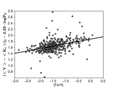
Figure 9: Plot of $(<V>-<K_{s}>)_{0}-2.33\cdot logP_{F}$ as a function of [Fe/H]. The solid line shows linear fit (equation (21)) with parameters (22).

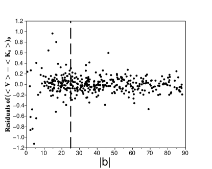
Figure 10: Plot of residuals of $(<V>-<K_{s}>)_{0}$ (equation (22)) as a function of $|b|$. Note the sharp increase of residuals at low Galactic latitudes ($|b|~{}\leq~{}25^{\circ}$)

.

Obviously, the 3D extinction model Drimmel et al. (2003) should perform better for objects at high Galactic latitudes and yield less accurate results in the vicinity of the Galactic equator. This is immediately apparent from the plot of residuals of equation (21) as a function of $|b|$ (Fig. (10)). Residuals can be seen to increase sharply at $|b|~{}\leq~{}25^{\circ}$. We therefore make a new least-squares fit leaving only stars with $|b|~{}>~{}25^{\circ}$:

$$(<V>-<K_{s}>)_{0}=(1.863\pm 0.024)$$ (23)

$$+(0.144\pm 0.016)\cdot[Fe/H]+2.33\cdot logP_{F},$$

with a scatter of $\sigma(<V>-<K_{s}>)_{0}$ = 0.11. This result implies, given the adopted metallicity-$<M_{V}>$ relation (17):

$$<M_{K_{s}}>=a_{v}-1.863+0.088(\pm 0.026)\cdot[Fe/H]-2.33\cdot logP_{F}$$ (24)

To make this relation as consistent as possible with the period-$<M_{K_{s}}>$ relation (6), we set $a_{v}-1.863+0.088\cdot(<[Fe/H]>)=-0.90$ (here $<[Fe/H]>$ = -1.419 is the average metallicity of sample stars), implying $a_{v}$ = 1.088 and hence:

$$<M_{V}>=1.088+0.232\cdot[Fe/H]$$ (25)

and

$$<M_{K_{s}}>=-0.775+0.088(\pm 0.026)\cdot[Fe/H]-2.33\cdot logP_{F}$$ (26)

We now assume that the WISE W1-band absolute magnitudes of RR Lyrae type variables depend both on metallicity and fundamentalised period as:

$$<M_{W1}>=a_{w}+b_{w}\cdot[Fe/H]+c_{w}\cdot logP_{F},$$ (27)

We subtract equation (27) from equation (18) to obtain (given that $(<K_{s}>-<W1>)_{0}=<M_{K_{s}}>-<M_{W1}>$):

$$(<K_{s}>-<W1>)_{0}=a_{kw}+b_{kw}\cdot[Fe/H]+c_{kw}\cdot logP_{F},$$ (28)

where $a_{kw}=a_{k}-a_{w}$, $b_{kw}=b_{k}-b_{w}$, and $c_{kw}=c_{k}-c_{w}$. We then use the least squares method to solve equation set (28) for stars with $|b|~{}>~{}25^{\circ}$:

$$(<K_{s}>-<W1>)_{0}=(0.021\pm 0.032)$$ (29)

$$-(0.017\pm 0.012)\cdot[Fe/H]-(0.039\pm 0.071)\cdot logP_{F},$$

with a scatter of $\sigma(<K_{s}>-<W1>)_{0}$ = 0.07. Both the [Fe/H] and $logP_{F}$ terms are statistically insignificant and we therefore seek the most simple solution setting $b_{kw}=0$ and $c_{kw}=0$ and leaving only the constant term:

$$(<K_{s}>-<W1>)_{0}=(0.056\pm 0.004)$$ (30)

with a scatter of $\sigma(<K_{s}>-<W1>)_{0}$ = 0.07 We thus derive, in view of relation (26), the following period-metallicity-$<M_{W1}>$ relation :

$$<M_{W1}>=-0.831+0.088(\pm 0.026)\cdot[Fe/H]-2.33\cdot logP_{F},$$ (31)

and the following $(<V>-<W1>)_{0}$ intrinsic colour calibration:

$$(<V>-<W1>)_{0}=1.919(\pm 0.024)$$

$$+0.144(\pm 0.016)\cdot[Fe/H]+2.33\cdot logP_{F},$$ (32)

for RR Lyrae type stars. We now refine this calibration by deriving it directly from the observed $(<V>-<W1>)$ colours assuming that the period-metallicity-$<M_{V}>$ relation has zero log $P_{F}$ slope and the metallicity slope equal to $b_{v}$=0.232$\pm$0.020, and the period-metallicity-$<M_{W1}>$ relation has the same log $P_{F}$ slope as the period-metallicity-$<M_{K_{s}}>$ relation (i.e., $c_{w}$=-2.33) and unknown metallicity slope:

$$(<V>-<W1>)_{0}=1.884(\pm 0.019)$$

$$+0.120(\pm 0.012)\cdot[Fe/H]+2.33\cdot logP_{F}$$ (33)

with a scatter of 0.086. We now use this calibration to determine the colour excesses $E(<V>-<W1>)=(<V>-<W1>)-(<V>-<W1>)_{0}$ for most of the stars at low Galactic latitudes ($|b|~{}\leq~{}25$) and convert these colour excesses into $E(B-V)$ values by the formula

$$E(B-V)=E(<V>-<W1>)/(R_{V}-R_{W1}),$$

where we adopt $R_{V}$ = 3.1 and $R_{W1}$ = 0.18 in accordance with Yuan et al. (2013). No intensity-mean $<W1>$ magnitudes are available for four stars with $|b|~{}\leq~{}25$. For these stars we use calibration (LABEL:VKS) to compute the colour excesses $E(<V>-<K_{s}>)=(<V>-<K_{s}>)-(<V>-<K_{s}>)_{0}$, which we convert into $E(B-V)$ values by the formula

$$E(B-V)=E(<V>-<K_{s}>)/(R_{V}-R_{K_{s}}),$$

where $R_{K_{s}}$ = 0.306 (Yuan et al., 2013). For the remaining stars (i.e., those at $|b|~{}>~{}25$) we adopt the $E(B-V)$ values $E(B-V)=A_{V}/R_{V}$ computed in terms of the 3D interstellar extinction model by Drimmel et al. (2003) via the iterative procedure described above.

The data used in this work (including the accurate coordinates, proper motions (with source and standard-error estimate), radial velocities (with source and standard errors), intensity-mean $V$-, $K_{s}$-, and $W1$-band magnitudes (with source and standard-error estimate), [Fe/H] (with source), period, and pulsation mode are listed in Table 2 (the full version will be available from the CDS). The columns of this table contain: (1) the GCVS name of the star; (2) and (3) - its J2000.0 equatorial coordinates $\alpha$ and $\delta$, respectively in decimal degrees; (4) the variability period in days; (5) the RR Lyrae type (AB or C); (6) and (7) the intensity-mean $V$-band magnitude ($<V>$) and its standard error ($\sigma<V>$), respectively; (8) the $V$-band interstellar extinction ($A_{V}$); (9) and (10) the metallicity [Fe/H] on the Zinn and West scale and its reference code (Ref.), respectively; (11) - (13) the intensity-mean $K_{s}$-band magnitude ($<K_{s}>$), its standard error ($\sigma<K_{s}>$), and reference code (Ref.), respectively; (14)-(15) the intensity-mean $W1$-band magnitude ($<W1>$) and its standard error ($\sigma<W1>$), respectively; (16)-(18) the average radial velocity ($V_{R}$), its standard error ($\sigma<V_{R}>$) (both in km/s), and reference code (Ref.), respectively; (19)-(20) the proper motion in right ascension ($\mu_{\alpha}$) and its standard error ($\sigma\mu_{\alpha}$) in mas/y, and (21)-22) the proper motion in right ascension ($\mu_{\delta}$) and its standard error ($\sigma\mu_{\delta}$) in mas/y.

Table 2: The first 10 lines of the catalogue of observational data for 403 Galactic field RR Lyrae variables. This is a sample of the full version, which is available in the online version of the article (see Supporting Information).

(1)	(2)	(3)	(4)	(5)	(6)	(7)	(8)	(9)	(10)	(11)	(12)	(13)
Name	$\alpha$	$\delta$	Period	Type	$<V>$	$\sigma<V>$	$A_{V}$	[Fe/H]	Ref.	$<K_{s}>$	$\sigma<K_{s}>$	Ref.
	degrees	degrees	(days)
SW And	005.929541	+29.401022	0.4423	AB	9.712	0.009	0.113	-0.38	1	8.509	0.035	11
XX And	019.364182	+38.950554	0.7229	AB	10.687	0.009	0.004	-2.01	1	9.411	0.035	11
XY And	021.676799	+34.068581	0.3988	AB	13.680	0.019	0.137	-0.92	1	12.892	0.040	11
ZZ And	012.395191	+27.022129	0.5546	AB	13.082	0.018	0.125	-1.58	1	11.834	0.035	11
AT And	355.628474	+43.014362	0.6170	AB	10.694	0.018	0.414	-0.97	2	9.090	0.036	11
BK And	353.775162	+41.102886	0.4216	AB	12.970	0.037	0.344	-0.08	1	11.663	0.040	11
CI And	028.784546	+43.765705	0.4848	AB	12.244	0.018	0.211	-0.83	1	10.929	0.035	11
DM And	353.003024	+35.196911	0.5916	AB	11.943	0.037	0.439	-2.32	1	10.575	0.038	11
DR And	016.294632	+34.218426	0.5328	AB	12.431	0.037	0.122	-1.48	1	11.332	0.035	11
NQ And	002.886174	+30.861319	0.6194	AB	99.000	99.000	0.165	-1.43	8	14.668	0.091	12
(Continued)
	(14)	(15)	(16)	(17)	(18)	(19)	(20)	(21)	(22)
Name	$<W1>$	$\sigma<W1>$	$V_{R}$	$\sigma V_{R}$	Ref.	$\mu_{\alpha}$	$\sigma\mu_{\alpha}$	$\mu_{\delta}$	$\sigma\mu_{\alpha}$
			(km/s)	(km/s)		(mas/yr)	(mas/yr)	(mas/yr)	(mas/yr)
SW And	8.464	0.009	-21.0	1.0	18	-7.6	1.1	-20.1	0.9
XX And	9.378	0.006	0.0	1.0	18	56.8	0.8	-35.0	0.7
XY And	12.617	0.005	-64.0	53.0	18	11.8	1.7	-8.3	2.4
ZZ And	11.795	0.010	-13.0	53.0	18	31.8	1.4	-15.3	1.6
AT And	9.012	0.004	-228.0	1.0	18	-9.5	0.5	-50.5	0.7
BK And	11.614	0.008	-17.0	7.0	19	4.9	1.2	-1.2	1.2
CI And	10.978	0.006	24.0	5.0	18	0.8	0.9	-1.9	0.9
DM And	10.471	0.012	-265.0	30.0	18	9.0	1.0	9.9	0.9
DR And	11.257	0.011	-81.0	30.0	18	28.2	1.1	-6.4	0.6
NQ And	14.850	0.044	-242.0	15.0	20	5.4	4.7	-4.2	4.4

4 Initial distances

We now again deredden the observed intensity-mean $<V>$, $<K_{s}>$, and $<W1>$ magnitudes using formulae (10–12) and the finally adopted $E(B-V)$ values. We then determine the initial (assumed) distances to most of the RR Lyrae stars of our sample based on the period-metallicity-$<M_{W1}>$ relation (31). We use the the period-metallicity-$<M_{K_{s}}>$ relation (26) to compute the distances to five stars with no intensity-mean $<W1>$ magnitudes.

Our working sample consists of all stars with simultaneously available $W1$-band intensity-mean magnitudes, metallicities, radial velocities, and UCAC4 proper motions (a total of 387 stars). Below we apply the method of statistical parallax to this sample to determine a correction $\Delta<M_{W1}>$ to the zero point of relation (31) so that

$$<M_{W1(true)}>=<M_{W1}(adopted)>+\Delta<M_{W1}>.$$ (34)

5 THE METHOD

Throughout this paper, we use the bimodal version of the classical maximum-likelihood statistical-parallax method (Murray, 1983) as described in Section 2.4 of Dambis (2009). In this case the likelihood function of obtaining all observations (apparent magnitudes, fundamental periods, metallicities, radial velocities, and proper motions of all stars of the sample studied) depends on fourteen parameters: (1) three components of the relative bulk motion of the objects of the first ($U_{0(1)}$, $V_{0(1)}$, and $W_{0(1)}$) and second ($U_{0(2)}$, $V_{0(2)}$, and $W_{0(2)}$) subsamples with respect to the Sun; (2) three diagonal components of velocity ellipsoid of the first ($\sigma V_{rg(1)}^{2}$, $\sigma V_{\varphi(1)}^{2}$, and $\sigma V_{\theta(1)}^{2}$) and second ($\sigma V_{rg(2)}^{2}$, $\sigma V_{\varphi(2)}^{2}$, and $\sigma V_{\theta(2)}^{2}$) subsamples, (3) the inverse distance-scale correction factor, $f$ (the same for both subsamples), and (4) the fraction $\alpha$ of stars that belong to the first subsample (in the bimodal case the fraction of stars that belong to the second subsample is evidently equal to 1-$\alpha$).

6 Results

Layden (1995) and Layden et al. (1996) showed that the kinematic population of RR Lyraes in our Galaxy breaks conspicuously into two subclasses: halo and thick-disc stars. As we pointed out in the previous section, we use the model incorporating explicitly the bimodal velocity distribution and compute 14 unknown parameters simultaneously. Table 3 lists the results based on the entire sample.

Table 3: Kinematical parameters and $W1$-band absolute-magnitude correction of Galactic field RR Lyrae variables inferred from the entire sample (387 stars).

Population		Fraction of the sample	$U_{0}$	$V_{0}$	$W_{0}$	$\sigma V_{R}$	$\sigma V_{\varphi}$	$\sigma V_{\theta}$
		($\alpha$ and 1-$\alpha$)				km/s
Halo		0.796	-6.8	-210.3	-8.9	146.7	98.8	96.5
		$\pm$ 0.028	$\pm$ 8.9	$\pm$ 9.0	$\pm$ 5.8	$\pm$ 7.5	$\pm$ 5.3	$\pm$ 5.1
Disc		0.204	-11.3	-38.9	-15.6	45.2	37.0	26.6
		$\pm$ 0.028	$\pm$ 6.7	$\pm$ 6.5	$\pm$ 4.2	$\pm$ 6.8	$\pm$ 5.2	$\pm$ 4.5
					$\Delta<M_{W1}>$	$=$	+0.065	$\pm$ 0.083

Note, however, that despite its mathematical sophistication, our analysis has at least one weak point: it assumes that all the quantities characterising the velocity distribution ( $U_{0}$, $V_{0}$, $W_{0}$, $\sigma V_{R}$, $\sigma V_{\theta}$, and $\sigma W$ for the halo and thick-disc subpopulations and their respective fractions) are location independent. This is evidently not true, and the corresponding effect cannot be neglected given the large spread of Galactocentric distances of sample stars (Fig. 11). To reduce the influence of this effect, we repeat our computations by applying the method to a trimmed sample: we leave only stars with Galactocentric distances that differ no more than 1.6 kpc from the provisionally adopted Galactocentric distance of the Sun ($R_{0}$ = 8 kpc): $6.4~{}kpc~{}\leq~{}R_{G}~{}\leq~{}9.6~{}kpc$. The corresponding results are presented in Table 4. Our result requires no absolute-magnitude zero point correction ($\Delta<M_{W1}>$ = +0.006 $\pm$ 0.088) and therefore we do not have to adjust the initial distances or intrinsic-colour calibrations (23) and (30), which depend on the adopted extinction values, which, in turn, depend on the adopted distances via the 3D interstellar extinction model by Drimmel et al. (2003).

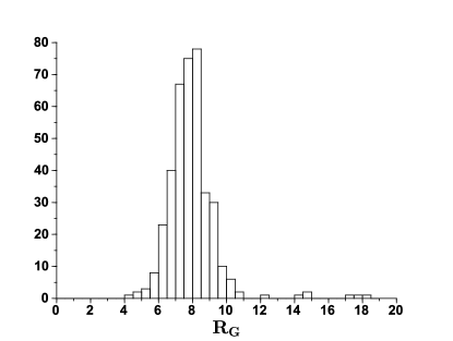
Figure 11: Histogram of Galactocentric distances of sample stars

.

Table 4: Kinematical parameters and $W1$-band absolute-magnitude correction of Galactic field RR Lyrae variables based on the bimodal solution (336 stars with Galactocentric distances in the interval from 6.4 to 9.6 kpc).

Population		Fraction of the sample	$U_{0}$	$V_{0}$	$W_{0}$	$\sigma V_{R}$	$\sigma V_{\varphi}$	$\sigma V_{\theta}$
		($\alpha$ and 1-$\alpha$)				km/s
Halo		0.777	-8.5	-214.0	-9.3	153.3	100.4	96.8
		$\pm$ 0.029	$\pm$ 9.4	$\pm$ 9.6	$\pm$ 6.2	$\pm$ 8.5	$\pm$ 5.8	$\pm$ 5.4
Disc		0.223	-12.0	-37.2	-17.0	47.0	36.7	27.2
		$\pm$ 0.029	$\pm$ 7.0	$\pm$ 6.1	$\pm$ 4.3	$\pm$ 6.9	$\pm$ 5.1	$\pm$ 4.4
					$\Delta<M_{W1}>$	$=$	+0.006	$\pm$ 0.088

To check our results for the eventual biases, we use the same procedure as that employed by Dambis (2009). We generate for every our solution a set of 400 simulated samples consisting of objects with exactly the same sky locations as those of stars in the real sample. We simulate the ”observed” parameters of each object (i.e., the distance, radial velocity, and proper-motion components) based on the distance of the corresponding star (which we divide by the inferred distance-scale correction factor $f$ plus the cosmic scatter), the mean velocity components (($U_{0}$, $V_{0}$, $W_{0}$) of one of the two subpopulations (chosen randomly in accordance with the inferred fractions $\alpha$ and 1-$\alpha$) with the corresponding velocity ellipsoid (defined by $\sigma V_{rg}$, $\sigma V_{\varphi}$, and $\sigma V_{\theta}$) superimposed. We finally add to the radial velocities and proper-motion components so computed the corresponding simulated random errors with zero means and variances determined by the standard errors of the actually observed quantities. We apply our bimodal method to each of the simulated samples to estimate the mean offsets of all the inferred parameters.

We find our method to yield unbiased estimates for all the parameters in the case considered, and therefore apply no corrections to our results. We adopt the parameters given by the solution based on the trimmed sample (Table4)as our final result, and, in particular, the corresponding corrected zero point for the infrared PL relation, which is is 0.026^m fainter than that the initially adopted value (see formula (31)), implying the following corrected W1-band period-metallicity-luminosity relation:

$$<M_{W1}>=-0.825(\pm 0.088)$$

$$+0.088(\pm 0.026)\cdot[Fe/H]-2.33\cdot logP_{F}.$$ (35)

We also apply the same zero-point correction to the V-band metallicity-luminosity relation given by formula (25) and the $K_{s}$-band period-metallicity-luminosity relation given by formula (26) to obtain the following corrected relations:

$$<M_{V}>=1.094(\pm 0.091)+0.232(\pm 0.020)\cdot[Fe/H]$$ (36)

and

$$<M_{K_{s}}>=-0.769(\pm 0.088)$$

$$+0.088(\pm 0.026)\cdot[Fe/H]-2.33\cdot logP_{F}.$$ (37)

The implied period-metallicity-luminosity relation for the CIT K band then is:

$$<M_{K_{CIT}}>=-0.750(\pm 0.088)+$$

$$0.088(\pm 0.026)\cdot[Fe/H]-2.33\cdot logP_{F}.$$ (38)

6.1 Comparison to earlier work

The only previous WISE W1-band luminosity calibration of RR Lyrae type variables is that of Klein et al. (2011), who found $<M_{W1}>=(0.421\pm 0.014)-(1.681\pm 0.147)\cdot log(P/0.50118day)$ with no evidence for metallicity term by computing posterior distances of 76 well observed RR Lyrae based on the optically constructed prior distances. Our PL relation is $\sim$ 0.16^m fainter at $P=0.50118$ and [Fe/H]=-1.5, and this is due entirely to the prior distance estimates adopted by the above authors, which are based on the $<M_{V}>$ - [Fe/H] relation $<M_{V}>$=0.93 + 0.23$\cdot$[Fe/H] (Chaboyer, 1999). The difference in the slope appears to be due to fact that Klein et al. (2011) do not fundamentalise the periods of RRc type stars. We believe this to be a questionable approach given that (a) RRc type stars form a well-defined period-shifted (by $\delta$ log($P$)=-0.127) branch of the $K$-band PL relation (see, e.g., Frolov & Samus (1998)) and (b) intrinsic $K_{s}$-W1 colours are practically constant for A-F type stars, implying that $<M_{W1}>$ may serve as a proxy for $<M_{Ks}>$ and that the period-$<M_{W}>$ relation should have practically the same slope as the period-$<M_{K_{s}}>$ relation (i.e., -2.33).

Our RR Lyrae $V$-band luminosity scale zero point ($<M_{V}>$=+0.72$\pm$0.09 at [Fe/H]=-1.6), albeit consistent with most of the analyses based on the method of statistical parallax, differs markedly from the most recent such study of c-type RR Lyrae variables by Kollmeier et al. (2012): they found $<M_{V,RRc}>$ = +0.52 $\pm$ 0.11 at a metallicity of [Fe/H] = -1.59, whereas formula (36) implies $<M_{V}>$ = +0.73$\pm$0.09 for the same metallicity. This can be compared with the statistical-parallax based estimates $<M_{V}>$ = +0.71$\pm$0.12 (Layden et al., 1996) and $<M_{V}>$ = +0.75$\pm$0.13 (Popowski & Gould, 1998a), both at [Fe/H]=-1.61; $<M_{V}>$ = +0.73$\pm$0.14 (Fernley et al., 1998a) at [Fe/H]=-1.53; $<M_{V}>$ = +0.69$\pm$0.10 (Tsujimoto, 1998) at [Fe/H]=-1.58; $<M_{V}>$ = +0.65$\pm$0.23 (Luri et al., 1998) at [Fe/H]=-1.51, and $<M_{V}>$ = +0.76–0.78$\pm$0.10 (Dambis & Rastorguev, 2001) at [Fe/H]=-1.60.

Our zero point of the $K$-band luminosity calibration is also consistent with the previous statistical-parallax determinations $<M_{K_{s}}>$ = -0.82$\pm$0.12 -2.33$\cdot$log($P_{F}$) (Dambis, 2003), $<M_{K_{s}}>$ = -0.89$\pm$0.09 -2.33$\cdot$log($P_{F}$) (Dambis & Vozyakova, 2004), $<M_{K_{s}}>$ = -0.94$\pm$0.06 -2.33$\cdot$log($P_{F}$) (Rastorguev, Dambis & Zabolotskikh, 2005), and $<M_{K_{s}}>$ = -0.818$\pm$0.08 -2.33$\cdot$log($P_{F}$) (Dambis, 2009) compared to $<M_{K_{s}}>$ = -0.901$\pm$0.09 -2.33$\cdot$log($P_{F}$) (formula (37) with [Fe/H] fixed at -1.5).

Both our $V$- and $K_{s}$-band absolute-magnitude calibrations agree well with the results obtained using the Baade-Wesselink method: $<M_{K}>$ = -0.88 -2.33$\cdot$log($P_{F}$) and $<M_{V}>$ = 1.02+0.16$\cdot$[Fe/H] (the latter implies $<M_{V}>$ = +0.76$\pm$0.03 at [Fe/H] = -1.6) (Jones et al., 1992) and $<M_{V}>$ = 0.98+0.20$\cdot$[Fe/H] (implying $<M_{V}>$ = +0.66$\pm$0.05 at [Fe/H] = -1.6) (Fernley et al., 1998b)).

At the same time, our RR Lyrae luminosity scale is inconsistent with HST trigonometric parallaxes of five RR Lyrae type variables: our $<M_{V}>$, $<M_{Ks}>$, and $<M_{W1}>$ zero points are 0.34$\pm$0.05, 0.32$\pm$0.05, and 0.34$\pm$0.05 fainter than those inferred by applying the reduced parallax method to the HST parallax data Benedict et al. (2011). The reason for such a discrepancy remains unclear.

Our $V$- and $K$- band luminosity scales are also appreciably fainter than the estimates based on analyses based on theoretical models (Bono et al., 2003; Catelan et al., 2004) and that defined by the period-metallicity-$<M_{K}>$ relation of Sollima et al. (2008): $<M_{K}>$=-1.07 - 2.38$\cdot$log $P_{F}$ +0.09$\cdot[Fe/H]_{ZW}$. The latter is tied to the HST parallax of RR Lyrae itself and is therefore naturally $\sim$0.3^m brighter than our period-metallicity-$<M_{K}>$ relation (see above). Note, however, that our metallicity slope, which is equal to +0.088$\pm$0.026, practically coincides with that of the relation derived by Sollima et al. (2008), but is appreciably shallower than the values of 0.231$\pm$0.012 and 0.277 estimates derived theoretically by Bono et al. (2003) and Catelan et al. (2004), respectively. We compare our metallicity-$<M_{V}>$ relation with the published ones in Fig 12. A similar comparison of period-$<M_{K}>$ relations (at [Fe/H]=-1.6) is made in Fig. 13.

We thus see that, as always before, the method of statistical parallax, like the Baade–Wesselink method, continues to yield RR Lyrae luminosities and distances that are at the lower end of the estimates obtained using various techniques. The cause of the discrepancies with other methods remains unknown and can hardly be attributed to photometric or astrometric errors given the dramatic improvement of the quality of the corresponding data both in terms of random errors and homogeneity. Neither can it be due to eventual systematic errors in the estimated amount of interstellar extinction, which is rather small for most of the RR Lyrae variables considered: its average value in the $V$ band is less than 0.2^m, and becomes negligible in the $K_{s}$ and $W1$ bands (0.019^m and 0.013^m, respectively). Furthermore, the $<M_{K_{s}}>$- and $<M_{W1}>$-band absolute magnitudes depend only slightly on metallicity and therefore metallicity errors are very unlikely to introduce any significant biases into these quantities. As shown by Popowski & Gould (1998a, b), the same is true for eventual radial-velocity errors and errors in the adopted kinematical model. We hope that the upcoming GAIA mission will finally resolve this controversy.

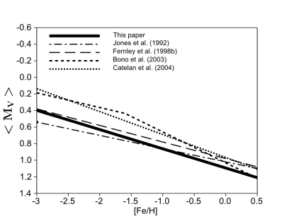
Figure 12: Comparison of our metallicity-$<M_{V}>$ relation (thick solid line) with published theoretical relations (Bono et al., 2003; Catelan et al., 2004) and relations based on the Baade–Wesselink method (Jones et al., 1992; Fernley et al., 1998b)

.

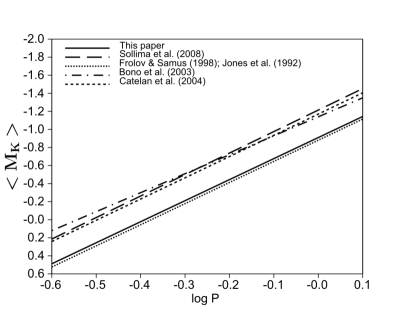
Figure 13: Comparison of our period-$<M_{K}>$ relation (solid line) with published theoretical relations (Bono et al., 2003; Catelan et al., 2004), a relation based on the Baade–Wesselink method (Jones et al., 1992), and two relations based on analyses of cluster RR Lyrae type stars (Frolov & Samus, 1998; Sollima et al., 2008)

.

The kinematical results obtained appear to be consistent with earlier statistical-parallax based results for RR Lyrae type stars ((Layden et al., 1996; Fernley et al., 1998a; Dambis & Rastorguev, 2001; Dambis, 2009; Kollmeier et al., 2012)) and with those of a recent analysis of the kinematics of BHB stars by halo stars by Kafle et al. (2012) (see Fig. 3 in their paper) and the fundamental kinematical study of halo stars by Carollo et al. (2007) (Supplemental Table 1), Carollo et al. (2010). As in our previous paper (Dambis, 2009), we find no signs of the outer halo population with retrograde rotation and large $\sigma V_{R}$ and $\sigma V_{\theta}$ velocity-dispersion components, which was to be expected given that our sample contains very few distant enough stars.

7 Distance-scale implications

Carney et al. (1995) estimated the distance to the Galactic centre to be $R_{0}$ = 7.80 $\pm$ 0.40 kpc based on the $K_{CIT}$-band photometry of Galactic bulge RR Lyraes and the assumed PL relation by Jones et al. (1992) (formula (4)). Pietrukowicz et al. (2012) find the average metallicity of Galactic bulge RR Lyrae type variables to be $<[Fe/H]>$ = -1.02 on the scale of Jurcsik (1995). This corresponds to $<[Fe/H]>_{ZW}$ = 1.028 $\cdot$ (-1.02) - 0.242 = -1.29 (Papadakis et al., 2000) on the Zinn & West (1984) metallicity scale. The resulting zero point of the (CIT) K-band PL relation for bulge RR Lyraes is then equal to -0.750 + 0.088$\cdot$(-1.29)=-0.863 (formula (38)), implying a solar Galactocentric distance of $R_{0}$ = (7.80 $\pm$ 0.40) $\cdot$ 10^{-0.2⋅(-0.863-(-0.88))} = 7.74 $\pm$ 0.40 kpc. Groenewegen et al. (2008) performed $K_{s}$-band observations of 39 type-II Cepheids and 37 RR Lyrae type stars in the Galactic bulge and estimated the RR Lyrae based distance to the Galactic centre to be $R_{0}$ = 7.87 $\pm$ 0.64 kpc $\pm$ 0.26 kpc using the period-metallicity-$<M_{K}>$ relation by Sollima et al. (2006). When recalibrated to our period-metallicity-$<M_{K}>$ relation, their RR Lyrae type star photometry yields a solar Galactocentric distance of $R_{0}$ = 7.19 $\pm$ 0.40 kpc $\pm$ 0.24 kpc. Based on OGLE II observations of stars in the Galactic bulge, Collinge, Sumi & Fabrycky (2006) find the average extinction-corrected intensity-mean $V$-band magnitude of RR Lyrae type stars in the Baade window to be $<V_{0}>$=15.44$\pm$0.05. Given the average metallicity of [Fe/H]=-1.0 of bulge stars, our [Fe/H]-$<M_{V}>$ relation (36) yields an absolute magnitude of $<M_{V}>$=+0.862, implying a GC distance modulus of $DM_{GC}$ = 14.58$\pm$0.10, or $R_{0}$=8.24$\pm$0.39 kpc. The average of the three estimates, $R_{0}$=7.73$\pm$0.36 kpc, is consistent both with the result based on the PL relation of type II Cepheids ($R_{0}$ = 7.64 $\pm$ 0.21 kpc (Feast et al., 2008) and $R_{0}$ = 7.99 $\pm$ 0.09 kpc (Groenewegen et al., 2008)) and with the direct estimate based on the orbital solution for the star S0-2 orbiting the supermassive black hole at the Galactic centre ($R_{0}$ = 8.28 $\pm$ 0.15 $\pm$ 0.29 kpc (Gillessen et al., 2009)).

If applied to the $K_{s}$-band photometry for 30 RR Lyrae type variables in Reticulum Dall’Ora et al. (2004) ([Fe/H]=-1.71), PML relation (37) yields a distance modulus of 18.22 $\pm$ 0.01 $\pm$ 0.09 ($D$ = 44.1 $\pm$ 0.2 $\pm$ 1.7 kpc) for this cluster, which is purportedly associated with the LMC. The $D_{Reticulum}/D_{LMCcentre}$ ratio can be estimated using a geometric model of the LMC, which is parametrised by the inclination $i$ and position angle of the line of nodes, $PA$ by the following formula:

$$D_{Reticulum}/D_{LMCcentre}=$$

$$cos~{}i/[cos~{}i~{}cos~{}\rho-sin~{}i~{}sin~{}\rho~{}sin(\Phi-PA)]$$ (39)

(van der Marel & Cioni, 2001), where $\rho$=11.4^∘ and $\Phi$=329^∘ are the angular distance and position angle of Reticulum with respect to the LMC, respectively (Schommer et al., 1992). Recent estimates of the LMC orientation parameters $PA$ and $i$ (van der Marel & Cioni, 2001; Olsen & Salyk, 2002; Nikolaev et al., 2004; Persson et al., 2004; Koerwer, 2009; Subramanian & Subramaniam, 2010, 2013) yield $D_{Reticulum}/D_{LMCcentre}$ ratios ranging from 0.959 to 1.041 corresponding to distance-scale corrections ranging from -0.09 to +0.09 with a mean of -0.01 and a standard deviation of 0.06. Hence the Reticulum distance derived yields an LMC distance modulus of 18.21 $\pm$ 0.01 $\pm$ 0.09 $\pm$ 0.06 ($D$ = 43.9 $\pm$ 0.2 $\pm$ 1.7 kpc $\pm$ 1.2 kpc). The $K_{s}$-band photometry of 10 RR Lyrae type stars in the inner regions of the LMC with spectroscopically measured [Fe/H] (Borissova et al., 2004) yields a distance modulus of 18.38 $\pm$ 0.04 $\pm$ 0.09 ($D$ = 47.4 $\pm$ 0.9 $\pm$ 2.0 kpc), and the similar data (65 stars) obtained by Szewczyk et al. (2008) imply an LMC distance modulus of 18.30 $\pm$ 0.02 $\pm$ 0.09 ($D$ = 45.7 $\pm$ 0.7 $\pm$ 1.9 kpc). The $V$-band intensity-mean magnitudes and metallicities of 89 RR Lyrae type stars determined by Gratton et al. (2004) analyzed in terms of our metallicity-$V$-band luminosity relation (36) yield an LMC distance modulus of 18.34 $\pm$ 0.02 $\pm$ 0.09 ($D$ = 46.6 $\pm$ 0.7 $\pm$ 2.1 kpc). We thus derive an average LMC distance modulus estimate of DM_LMC = 18.32 $\pm$ 0.09 ($D$ = 46.1 $\pm$ 2.0 kpc). This result is consistent with the estimate based on the PL relation of classical Cepheids and their HST trigonometric parallaxes: Feast et al. (2008) report $DM_{LMC}=18.39\pm 0.05$ as inferred from the estimate of Benedict et al. (2007) with the metallicity correction of Macri et al. (2006). Our LMC distance modulus also agrees with the recent LMC distance estimate based on type II Cepheids ($DM_{LMC}=18.37\pm 0.09$ (Feast et al., 2008)). However, it is $\sim$1.3-2.2$\sigma$ smaller than the DM_LMC = 18.46 $\pm$ 0.06 – 18.61 $\pm$ 0.05 ($D$ = 49.2 $\pm$ 1.4 kpc – 52.7 $\pm$ 1.2 kpc) estimates implied by $V$- and $K_{s}$-band photometry of RR Lyrae type variables in the LMC and HST triginometric parallaxes of five Galactic RR Lyraes (Benedict et al., 2011), and $\sim$1.5$\sigma$ smaller than the DM_LMC = 18.49 $\pm$ 0.05 ($D$ = 49.97 $\pm$ 1.11 kpc) estimate inferred from observations of eclipsing binaries (Pietrzyński et al., 2013) and the DM_LMC = 18.48 $\pm$ 0.04 ($D$ = 49.66 $\pm$ 0.92 kpc) estimate inferred from 3.6- and 4.5-$\mu$m observations of classical Cepheids made by Spitzer Space Telescope and calibrated by HST guide-star parallaxes of 10 Galactic Cepheids (Monson et al., 2012).

Clementini et al. (2009) analysed archival HST photometry of stars in the metal-poor globular cluster B514 in the M31 galaxy and identified 89 RR Lyrae type variables. Our $V$-band luminosity calibration (formula (36)) implies a distance modulus of $DM_{B514}$ = 24.32 $\pm$ 0.12 ($D$ = 731 $\pm$ 41 kpc)

Federici et al. (2012) collected and analysed archival HST $BVI$ photometry for 48 globular clusters in the M31 galaxy. They determined the apparent horizontal-branch $V$-band magnitudes, $M_{V}(HB)$, and estimated the reddenings and metallicities of these clusters by comparing their observed colour-magnitude diagrams to the colour-magnitude diagram ridge lines of a set of Galactic reference globular clusters. Given that in a globular cluster $M_{V}(HB)$ = $<M_{V}(RRLyr)>$, we apply formula (36) to the data of Federici et al. (2012) to obtain an M31 distance modulus estimate of $DM_{M31}$ = 24.201 $\pm$ 0.014 $\pm$ 0.090 ($D$ = 692 $\pm$ 5 $\pm$ 28 kpc).

When applied to the results of an an extensive survey of RR Lyrae type variables in three fields along the major axis of the M33 galaxy by Yang et al. (2010), our $V$-band metallicity-luminosity relation (36) yields a distance modulus of $DM_{M33}$ = 24.36 $\pm$ 0.09 ($D$ = 745 $\pm$ 31 kpc).

Table 5 summarises the RR Lyr (or horizontal-branch) based distance estimates mentioned above, and other such distance estimates for a number of Local-Group galaxies. Our distance moduli are, on the average, 0.13 smaller than most recent published estimates. This difference is due mostly to the difference in the zero points of the underlying calibrations, which are generally based on some reference LMC distance modulus (cf. our $DM_{LMC}$ = 18.34$\pm$0.09 with the estimates $DM_{LMC}(Freedman)$ = 18.477$\pm$0.033 and $DM_{LMC}(Riess)$ = 18.486$\pm$0.065 adopted by Freedman et al. (2012) and Riess et al. (2011), respectively.

Table 5: Distance to Local Group galaxies estimated from the data for RR Lyr type variables (RR) or horizontal-branch stars (HB) using relations (36) (for $V$-band data) or (37) (for $K$-band data). Published distance moduli are representative only to give an idea of (generally) most recent previous estimates.

Galaxy	Objects	Filter	Instrument	Distance	Distance,	Data	Rem.	Published	Ref.
				modulus	kpc	ref.		DM
Milky Way	RR	$K$	4-m CTIO	14.44$\pm$0.11	7.74$\pm$0.40	1
Milky Way	RR	$K_{s}$	ESO NTT	14.29$\pm$0.11	7.19$\pm$0.37	1a
(Galactic	RR	$V$	OGLE-II	14.58$\pm$0.10	8.24$\pm$0.39	3
centre)			Mean:	14.44$\pm$0.10	7.73$\pm$0.36			14.59$\pm$0.09	31
LMC	RR	$K_{s}$	ESO VLT,	18.38$\pm$0.10	47.4$\pm$2.2	4
			ESO NTT
LMC	RR	$K_{s}$	ESO NTT	18.30$\pm$0.09	45.7$\pm$1.9	5
LMC	RR	$K_{s}$	ESO NTT	18.21$\pm$0.11	43.9$\pm$2.1	6	a
LMC	RR	$V$	ESO VLT	18.34$\pm$0.09	46.6$\pm$2.1	7
			Mean:	18.32$\pm$0.09	46.1$\pm$2.0			18.477$\pm$0.033	26
SMC	RR	$V$	OGLE-III	18.72$\pm$0.09	55.5$\pm$2.3	8
SMC	RR	$K_{s}$	ESO NTT	18.71$\pm$0.17	55.2$\pm$3.5	9
			Mean:	18.72$\pm$0.09	55.5$\pm$2.3			18.93$\pm$0.10	27
M31	RR	$V$	HST	24.32$\pm$0.12	731$\pm$41	10	b
M31	HB	$V$	HST	24.20$\pm$0.09	692$\pm$28	11
			Mean:	24.24$\pm$0.09	705$\pm$30			24.38$\pm$0.06	23
			M31	satellites
M32	RR	$V$	HST	24.26$\pm$0.12	711$\pm$40	12		24.51$\pm$0.14	28
NGC147	RR	$V$	HST	24.00$\pm$0.16	631$\pm$48	13		24.26$\pm$0.06	29
And I	RR	$V$	HST	24.23$\pm$0.11	701$\pm$36	14		24.31$\pm$0.05	29
And II	RR	$V$	HST	23.93$\pm$0.11	611$\pm$32	15		24.00$\pm$0.05	29
And III	RR	$V$	HST	24.18$\pm$0.11	685$\pm$35	14		24.30$\pm$0.06	29
And V	RR	$V$	HST	24.41$\pm$0.09	762$\pm$32	16		24.35$\pm$0.06	29
And VI	RR	$V$	HST	24.37$\pm$0.09	748$\pm$32	17		24.47$\pm$0.07	30
And XI	RR	$V$	HST	24.17$\pm$0.09	682$\pm$29	18		24.33$\pm$0.05	18
And XIII	RR	$V$	HST	24.46$\pm$0.09	780$\pm$33	18		24.62$\pm$0.07	18
M33	RR	$V$	HST	24.36$\pm$0.09	745$\pm$31	19		24.53$\pm$0.11	24
IC1613	RR	$V$	HST	24.19$\pm$0.09	689$\pm$29	20		24.34$\pm$0.03	25
Sex dSph	RR	$V$	3.6-m CFH	19.74$\pm$0.21	88.7$\pm$8.9	21		19.90$\pm$0.06	21
Cetus	RR	$V$	HST	24.37$\pm$0.09	748$\pm$32	22		24.46$\pm$0.12	22
Tucana	RR	$V$	HST	24.66$\pm$0.09	855$\pm$36	22		24.74$\pm$0.12	22

Data sources: 1. Carney et al. (1995); 2. Groenewegen et al. (2008); 3. Collinge, Sumi & Fabrycky (2006); 4. Borissova et al. (2004);

5. Szewczyk et al. (2008); 6. Dall’Ora et al. (2004); 7. Gratton et al. (2004); 8. Kapakos & Hatzidimitriou (2012);

9. Szewczyk et al. (2009); 10. Clementini et al. (2009); 11. Federici et al. (2012); 12. Sarajedini (2012);

13. Yang & Sarajedini (2010); 14. Pritzl et al. (2005); 15. Pritzl et al. (2004); 16. Mancone & Sarajedini (2008);

17. Pritzl et al. (2002); 18. Yang & Sarajedini (2012); 19. Yang et al. (2010); 20. Bernard et al. (2010);

21. Lee et al. (2003); 22. Bernard et al. (2009); 23. Riess, Fliri & Valls-Gabaud (2012) (classical Cepheids);

24. Scowcroft et al. (2009) (classical Cepheids); 25. Tammann, Reindl & Sandage (2011) (classical Cepheids);

26. Freedman et al. (2012) (classical Cepheids); 27. Inno et al. (2013); 28. Fiorentino et al. (2010);

29. Conn et al. (2012) (tip of the red-giant branch); 30. McConnachie et al. (2005) (tip of the red-giant branch);

31. Gillessen et al. (2009).

Remarks: a. Reticulum globular cluster. It may be rather distant from the centre of the LMC

and we therefore use a geometric model to estimate the distance to the LMC centre (see text). b. B514 globular cluster.

8 Rotation of the RR Lyrae populations

Our estimate for the distance to the Galactic center, $R_{0}$=7.73$\pm$0.36 kpc, combined with the proper motion of Sgr A^∗ along Galactic longitude, $\mu_{SgrA^{*}}$ = 6.379 $\pm$ 0.026 mas/yr (Reid & Brunthaler, 2004), implies a solar velocity of $V_{\cdot}$=234$\pm$10 km/s. It follows from this that the halo RR Lyrae population exhibits marginal prograde rotation with a velocity of 20$\pm$15 km/s. The thick-disc RR Lyrae population rotates at a velocity of 193$\pm$13 km/s.

9 Cosmology

Our result, if taken at face value, would upscale the Hubble constant as estimated by Freedman et al. (2012) ($H_{0}$ = 74.3 $\pm$ 2.1 km/s/Mpc) to $H_{0}$ = 80.0 $\pm$ 3.4 km/s/Mpc, and imply, if combined with $\Omega_{\Lambda}$= 0.74$\pm$0.02 (Mohlabeng & Ralston, 2013) based on an analysis of a sample of 580 type Ia supernovae in terms of a flat, LCDM cosmological model, an expansion age of 12.5 Gyr, which is consistent with the globular-cluster ages of 12–13 Gyr (Carretta et al., 2000).

10 Conclusions

We collected homogenized data for 403 local Galactic field RR Lyrae variables: intensity-mean $V$-band, 2MASS $K_{s}$-band, and WISE $W1$-band magnitudes for 384, 403, and 398 stars, respectively; metallicity estimates on the Zinn & West (1984) scale for 402 stars, UCAC4 proper motions for 393 stars, as well as radial velocities and interstellar-extinction estimates for all 403 stars. We used the photometric data combined the 3D interstellar extinction model by Drimmel et al. (2003) to calibrate RR Lyrae star colours in terms of fundamental period and metallicity and used these calibrations to determine the log $P_{F}$ and metallicity slopes of the 2MASS $K_{s}$-band and WISE $W1$-band infrared period-metallicity-luminosity relations. We performed a bimodal statistical-parallax solution on the subsample of stars with both WISE $W1$-band intensity-mean magnitudes and UCAC4 proper motions available. We found the velocity components (relative to the Sun) of the halo and thick-disc populations along the direction of Galactic rotation to be $V_{0}(Halo)$=-214$\pm$10 km/s and $V_{0}(Disc)$=-37$\pm$6 km/s, respectively. The inferred velocity-ellipsoid components of are ($\sigma V_{R}(Halo),\sigma V_{\phi}(Halo),\sigma V_{\theta}(Halo)$) = $(153\pm 9,101\pm 6,96\pm 5)$ km s^-1 and ($\sigma V_{R}(Disc),\sigma V_{\theta}(Disc),\sigma W(Disc)$) = $(46\pm 7,37\pm 5,27\pm 4)$ km s^-1 for the halo and thick-disc, respectively, and the fraction of thick-disc stars, 0.22 $\pm$ 0.03. Our kinematical results agree well with those of other studies, and our final IR period-metallicity-luminosity relations and the $V$-band metallicity-luminosity relation are consistent with most of the previous statistical-parallax based estimates (with the exception of the statistical-parallax analysis of c-type RR Lyrae variables by Kollmeier et al. (2012)) and the results of the application of the Baade–Wesselink method, but generally fainter than implied by the results obtained using other methods. The distance moduli of Local Group galaxies estimated using our derived IR and optical luminosity calibrations are, on the average, 0.13 smaller than recently published determinations, implying a Hubble constant of $\sim$ 80 km/s and a rather small – 12.5 Gyr–expansion age of the Universe.

11 Acknowledgements

We thank the reviewer, Prof. G. Bono, for his valuable comments, which improved the final version of the paper. This publication makes use of data products from the Two Micron All Sky Survey, which is a joint project of the University of Massachusetts and the Infrared Processing and Analysis Center/California Institute of Technology, funded by the National Aeronautics and Space Administration and the National Science Foundation, and from the Wide-field Infrared Survey Explorer, which is a joint project of the University of California, Los Angeles, and the Jet Propulsion Laboratory/California Institute of Technology, funded by the National Aeronautics and Space Administration. This research has made use of NASA’s Astrophysics Data System. This work is supported by the Russian Foundation for Basic Research (projects nos. 13-02-00203-a and 11-02-00608-a). AYK and RS acknowledge the support from the National Research Foundation (NRF) of South Africa

References

- Anthony-Twarog & Twarog (1994) Anthony-Twarog B.J., Twarog B. A., 1994, AJ, 107, 1577
- Beers et al. (2000) Beers T. C., Chiba M., Yoshii Y., Platais I., Hanson R. B., Fuchs B., Rossi S., 2000, AJ, 119, 2866
- Benedict et al. (2007) Benedict G. F., McArthur B. E., Feast M. W., Barnes T. G., Harrison T. E., Patterson R. J., Menzies J. W., Bean J. L., Freedman W. L., 2007, AJ, 133, 1810
- Benedict et al. (2011) Benedict G. F., McArthur B. E., Feast M. W., Barnes Th. G., Harrison Th. E., Bean J. L., Menzies J. W., Chaboyer B., Fossati L., Nesvacil N., Smith H. A., Kolenberg K., Laney C. D., Kochukhov O., Nelan E.P., Shulyak D.V., Taylor D., Freedman W.L., 2011, AJ, 142, 187
- Berdnikov et al. (2011a) Berdnikov L. N., Kniazev A. Y., Sefako R., Kravtsov V. V., Dambis A. K., 2011, Observatory, 131, 315
- Berdnikov et al. (2011b) Berdnikov L. N., Kniazev A. Y., Sefako R., Kravtsov V. V., Dambis A. K., 2011, Observatory, 131, 386
- Berdnikov et al. (2012) Berdnikov L. N., Vozyakova O. V., Kniazev A. Yu., Kravtsov V. V., Dambis A. K., Zhuiko S. V., 2012, Astron. Rep., 56, 290
- Bernard et al. (2009) Bernard E. J., Monelli M., Gallart C., Drozdovsky I., Stetson P. B., Aparicio A., Cassisi S., Mayer L., Cole A. A., Hidalgo S. L., Skillman E. D., Tolstoy E., 2009, ApJ, 699, 1742
- Bernard et al. (2010) Bernard E. J., Monelli M., Gallart C., Aparicio A., Cassisi S., Drozdovsky I., Hidalgo S. L., Skillman E. D., Stetson P. B., 2010, ApJ, 712, 1259
- Bookmeyer et al. (1977) Bookmeyer B.B., Fitch W. S., Lee T. A., Wisniewski W. Z., Johnson H. L., 1977, Rev. Mex. A. A., 2, 235
- Bono et al. (2003) Bono G., Caputo F., Castellani V., Marconi M., Storm J., Degl’Innocenti S., 2003, MNRAS, 344, 1091
- Borissova et al. (2004) Borissova J., Minniti D., Rejkuba M., Alves D., Cook K. H., Freeman, K. C., 2004, A&A, 423, 97
- Cacciari (2013) Cacciari C., 2013, Advancing the Physics of Cosmic Distances, IAU Symposium 289, Proceedings of the 289th Symposium of the International Astronomical Union Held in Beijing, China, August 27 31, 2012. Edited by de Grijs, R., p. 101
- Cacciari et al. (1992) Cacciari C., Clementini G., Fernley J. A., 1992, ApJ, 396, 219.
- Carney et al. (1995) Carney B. W., Fulbright J. P., Terndrup D. M., Suntzeff N. B., Walker A. R., 1995, AJ, 116, 1674
- Carollo et al. (2007) Carollo D., Beers T. C., Lee Y. S., Chiba M., Norris J. E., Wilhelm R., Sivarani T., Marsteller B., Munn J. A., Bailer-Jones C. A. L., Fiorentin P. R., York D. G., 2007, Nature, 450, 1020
- Carollo et al. (2010) Carollo D., Beers T.C., Chiba M., Norris J. E., Freeman K. C., Lee Y. S., Ivezić Ž., Rockosi C. M., Yanny, B., 2010, ApJ, 712, 692
- Carretta et al. (2000) Carretta E., Gratton R., Clementini G., Fusi Pecci F., 2000, ApJ, 533, 215
- Catelan et al. (2004) Catelan, M., Pritzl, B. J., Smith, H. A., 2004, ApJS,154, 633
- Chaboyer (1999) Chaboyer, B. 1999, Post-Hipparcos Cosmic Candles, ed. A. Heck & F. Caputo (Dordrecht: Kluwer), 111
- Clementini et al. (2009) Clementini G., Contreras R., Federici L., Cacciari C., Merighi R., Smith Horace A., Catelan Marcio, Fusi Pecci F., Marconi M., Kinemuchi K., Pritzl B.J., 2009, ApJL, 704, L103
- Clube & Dawe (1980) Clube S.V., Dawe J.A., 1980, MNRAS, 190, 591
- Collinge, Sumi & Fabrycky (2006) Collinge M.J, Sumi T., Fabrycky D., 2006, ApJ, 651, 197
- Conn et al. (2012) Conn A. R., Ibata R. A., Lewis G. F., Parker Q. A., Zucker D. B., Martin N. F., McConnachie A. W., Irwin M. J., Tanvir N., Fardal M. A., Ferguson A. M. N., Chapman S. C., Valls-Gabaud D., 2012, ApJ, 758, 11
- Cutri et al. (2003) 2MASS All-Sky Catalog of Point Sources Cutri R. M., Skrutskie M. F., van Dyk S., Beichman C. A., Carpenter J. M., Chester T., Cambresy L., Evans T., Fowler J., Gizis J., Howard E., Huchra J., Jarrett T., Kopan E. L., Kirkpatrick J. D., Light R. M., Marsh K. A., McCallon H., Schneider S., Stiening R., Sykes M., Weinberg M., Wheaton W. A., Wheelock S., Zacarias N., 2003, The IRSA 2MASS All-Sky Point Source Catalog, NASA/IPAC Infrared Science Archive. http://irsa.ipac.caltech.edu/applications/Gator/
- Cutri et al. (2012) Cutri R.M. et al. 2012, VizieR Online Data Catalog, II/311
- Dall’Ora et al. (2004) Dall’Ora M., Storm J., Bono G., Ripepi V., Monelli M., Testa V., Andreuzzi G., Buonanno R., Caputo F., Castellani V., Corsi C. E., Marconi G., Marconi M., Pulone L., Stetson P.B., 2004, ApJ, 610, 269
- Dambis (2003) Dambis A.K., 2003, Galactic and Stellar Dynamics, Proceedings of JENAM 2002, held in Porto, Portugal, 3-6 September, 2002. Edited by C. M. Boily, P. Pastsis, S. Portegies Zwart, R. Spurzem and C. Theis, EAS Publications Series, 10, 55.
- Dambis (2009) Dambis A.K., 2009, MNRAS, 396, 553
- Dambis & Rastorguev (2001) Dambis A.K., Rastorguev, A.S., 2001, Pis’ma Astron. Zh., 27, 132
- Dambis & Vozyakova (2004) Dambis A.K., Vozyakova, O.V., 2004, Variable Stars in the Local Group, IAU Colloquium 193, Proceedings of the conference held 6-11 July, 2003 at Christchurch, New Zealand. Edited by Donald W. Kurtz and Karen R. Pollard. ASP Conference Proceedings, 310, 128.
- Day et al. (2002) Day A.S., Layden A.C., Hoard D.W., Brammer G., Cooksey K., Cuadra J., Holmes S., Labbe E., Montez R., Jr., 2002, PASP, 114, 645
- Drimmel et al. (2003) Drimmel R., Cabrera-Lavers A., Lopez-Corredoira M., 2003, A&A, 409, 205
- ESA (1997) ESA, 1997, The Hipparcos and Tycho Catalogues (ESA SP-1200). Nordwijk: ESA
- Feast et al. (2008) Feast M.W., Laney C.D., Kinman Th.D., van Leeuwen F., Whitelock P.A., 2008, MNRAS, 386, 2115
- Federici et al. (2012) Federici L., Cacciari C., Bellazzini M., Fusi Pecci F., Galleti S., Perina S., 2012, A&A, 544, 1459
- Fernley & Barnes (1997) Fernley J., Barnes T. G., 1997, A&AS, 125, 313
- Fernley et al. (1998a) Fernley J., Barnes T.G., Skillen I., Hawley S.L., Hanley C.J., Evans D.W., Solano E., Garrido R., 1998, AA, 330, 515
- Fernley et al. (1998b) Fernley J., Skillen I., Carney B. W., Cacciari C., Janes K., 1998, MNRAS, 293, L61
- Fiorentino et al. (2010) Fiorentino G., Monachesi A., Trager S.C., Lauer T.R., Saha A., Mighell K.J., Freedman W., Dressler A., Grillmair C., Tolstoy E., 2010, ApJ, 708, 817
- Fitch et al. (1967) Fitch W.S., Wisniewski W.Z., Johnson H.L., 1966, Comm. Lunar Plan. Lab., 5, 71
- For et al. (2011) For B.-Q., Preston G.W., Sneden Ch., 2011, ApJS, 194, 38
- Freedman et al. (2012) Freedman W.L., Madore B.F., Scowcroft V., Burns Ch., Monson A., Persson S.E., Seibert M., Rigby J., 2012, ApJ, 758, 24
- Frolov & Samus (1998) Frolov M. S., Samus N. N., 1998, Pis’ma Astron. Zh., 24, 509
- Gillessen et al. (2009) Gillessen S., Eisenhauer F., Fritz T. K., Bartko H., Dodds-Eden K., Pfuhl O., Ott T., Genzel R., 2009, ApJL, 707, 114
- Gould & Popowski (1998) Gould, A., Popowski P., 1998, ApJ, 508, 844
- Gratton et al. (2004) Gratton R.G., Bragaglia A., Clementini G., Carretta E., Di Fabrizio L., Maio M., Taribello E., 2004. A&A, 421, 937
- Groenewegen et al. (2008) Groenewegen M.A.T., Udalski A., Bono G., 2008, A&A, 481, 441
- Hawley et al. (1986) Hawley S.L., Jeffreys W.H., Barnes T.G.,III, Wan L., 1986, AJ, 302, 626
- Hemenway (1975) Hemenway M.K., 1975, AJ, 80, 199
- Inno et al. (2013) Inno L., Matsunaga N., Bono G., Caputo F., Buonanno R., Genovali K., Laney C. D., Marconi M., Piersimoni A. M., Primas F., Romaniello M., 2013, ApJ, 764, 84
- Jeffery et al. (2007) Jeffery E.J., Barnes Th.G., III, Skillen I., Montemayor Th.J., 2007, ApJS, 171, 512
- Jones et al. (1992) Jones R. V., Carney B. W., Storm J., Latham D., 1992, ApJ, 385, 646
- Jones et al. (1996) Jones R. V., Carney B. W., Storm J., Fulbright J.P., 1996, PASP, 108, 877
- Jurcsik (1995) Jurcsik J., 1995, AcA, 45, 653
- Kafle et al. (2012) Kafle P.R., Sharma S., Lewis G.F., Bland-Hawthorn, J., 2012, ApJ, 98
- Kapakos & Hatzidimitriou (2012) Kapakos E., Hatzidimitriou D., 2012, MNRAS, 426, 2063
- Kemper (1982) Kemper E., 1982, AJ, 87, 1395
- Kinemuchi et al. (2006) Kinemuchi K., Smith H.A., Woźniak P.R., McKay T.A., ROTSE Collaboration, 2006, AJ, 132, 1202
- Kinman (1961) Kinman T.D., 1961, RGOB, 37, 151
- Kinman (2002) Kinman T.D. 2002, IBVS, 5311, 1
- Kinman & Brown (2010) Kinman T.D., Brown W.R. 2010, IBVS, 5935, 1
- Kinman (1982) Kinman T.D., Mahaffey C.T., Wirtanen C.A., 1982, AJ, 87, 314
- Kinman et al. (2007) Kinman T. D., Cacciari C., Bragaglia A., Buzzoni A., Spagna, A. 2007, MNRAS, 375, 1381
- Kinman et al. (2012) Kinman T. D., Cacciari C., Bragaglia A., BSmart R., Spagna, A. 2012, MNRAS, 422, 2116
- Klein et al. (2011) Klein Ch.R., Richards J.W., Butler N.R., Bloom J.S., 2011, ApJ, 738, 185
- Koerwer (2009) Koerwer J.F., 2009, AJ, 138, 1
- Kollmeier et al. (2012) Kollmeier J.A., Szczygiel D.M., Burns C.R., Gould A., Thompson I.B., Preston G.W., Sneden C., Crane J.D., Dong S., Madore B.F., Morrell N., Prieto J.L., Shectman S., Simon J.D., Villanueva E., 2012arXiv1208.2689K
- Layden (1994) Layden A.C., AJ, 1994, 108, 1016
- Layden (1995) Layden A.C., AJ, 1995, 110, 2288
- Layden (1997) Layden A.C., PASP, 1997, 109, 524
- Layden et al. (1996) Layden A.C., Hanson R.B., Hawley S.L., Klemola A.R., Hanley C.J., 1996, AJ, 112, 2110
- Lee et al. (2003) Lee Myung Gyoon, Park Hong Soo, Park Jang-Hyun, Sohn Young-Jong, Oh Seung Joon, Yuk In-Soo, Rey Soo-Chang, Lee Sang-Gak, Lee Young-Wook, Kim Ho-Il, Han Wonyong, Park Won-Kee, Lee Joon Hyeop, Jeon Young-Beom, Kim Sang Chul, 2003, AJ, 126, 2840
- Lub (1977) Lub J., 1977, A&AS, 29, 345
- Luri et al. (1998) Luri X., Gomez A. E., Torra J., Figueras F., Mennessier M. O., AA, 1998, 335, L81
- Luri et al. (1996) Luri X., Mennessier M. O., Torra J., Figueras F., AA, 1996, 117, 405
- Macri et al. (2006) Macri L.M., Stanek K.Z., Bersier D., Greenhill L.J., Reid M.J., 2006, ApJ, 652, 1133
- Maintz (2005) Maintz, G., 2005, A&A 442, 381
- Mancone & Sarajedini (2008) Mancone C., Sarajedini A., 2008, AJ, 136, 1913
- McConnachie et al. (2005) McConnachie A. W., Irwin M. J., Ferguson A.M.N., Ibata R.A., Lewis G.F., Tanvir N., 2005, MNRAS, 356, 979
- Mohlabeng & Ralston (2013) Mohlabeng G.M., Ralston J.P., 2013, 2012arXiv1303.0580M
- Monson et al. (2012) Monson A.J., Freedman W.L., Madore B.F., Persson S. E., Scowcroft V., Seibert M., Rigby J.R., 2012, ApJ, 759, 146
- Morgan et al. (2007) Morgan S.M., Wahl J.N., Wieckhorst R.M. 2007, MNRAS, 374, 1421
- Murray (1983) Murray C.A., 1983, Vectorial Astrometry, (Bristol: A.Hilger)
- (85) Numerical Algorithm Library http://num-anal.srcc.msu.ru/
- Nikolaev et al. (2004) Nikolaev S., Drake A.J., Keller S.C., Cook K. H., Dalal N., Griest K., Welch D. L., Kanbur S. M., 2004, ApJ, 601, 260
- Norris (1986) Norris J., 1986, ApJS, 61, 667
- Olsen & Salyk (2002) Olsen K.A.G., Salyk C., 2002, AJ, 124, 2045
- Papadakis et al. (2000) Papadakis I., Hatzidimitriou D., Croke B. F. W., Papamasto-rakis I., 2000, AJ, 119, 851
- Pavlovskaya (1953) Pavlovskaya E.D., 1953, Peremennye Zvezdy, 9, 349
- Pel (1976) Pel J.W., 1976, Ph.D. Thesis, Leiden University
- Persson et al. (2004) Persson S.E., Madore B.F., Krzemiński W., Freedman W.L., Roth M., Murphy D.C., 2004, AJ, 128, 2239
- Pier et al. (2003) Pier J. R., Saha A., Kinman T. D., 2003, IBVS, 5459, 1
- Pietrukowicz et al. (2012) Pietrukowicz P., Udalski A., Soszyński I., Nataf D. M., Wyrzykowski Ł., Poleski R., Kozłowski S., Szymański M. K., Kubiak M., Pietrzyński G., Ulaczyk K., 2012, ApJ, 750, 169
- Pietrzyński et al. (2013) Pietrzyński G., Graczyk D., Gieren W., Thompson I. B., Pilecki B., Udalski A., Soszyński I., Kozłowski S., Konorski P., Suchomska K., Bono G., Moroni P. G. Prada, Villanova S., Nardetto N., Bresolin F., Kudritzki R. P., Storm J., Gallenne A., Smolec R., Minniti D., Kubiak M., Szymański M.K., Poleski R., Wyrzykowski Ł., Ulaczyk K., Pietrukowicz P., Górski M., Karczmarek P., 2013, Nature, 495, 76
- Pojmanski (2002) Pojmanski, G., 2002, Acta Astronomica, 52, 397
- Popowski & Gould (1998a) Popowski P., Gould A., 1998, ApJ, 506, 259
- Popowski & Gould (1998b) Popowski P., Gould A., 1998, ApJ, 506, 271
- Pritzl et al. (2002) Pritzl B.J., Armandroff T.E., Jacoby G.H., Da Costa G.S., 2002, AJ, 124, 1464
- Pritzl et al. (2004) Pritzl B.J., Armandroff T.E., Jacoby G.H., Da Costa G.S., 2004, AJ, 127, 318
- Pritzl et al. (2005) Pritzl B.J., Armandroff T.E., Jacoby G.H., Da Costa G.S., 2005, AJ, 129, 2232
- Pshenichnyi & Redkovskii (1976) Pshenichnyi B. N., Redkovskii N.N., 1976, Zhurnal Vychislitelmoi Matematiki i Matematicheskoi Fiziki, 16, 1388
- Rastorguev, Dambis & Zabolotskikh (2005) Rastorguev A. S., Dambis A. K., Zabolotskikh M. V., 2005, in The ThreeDimensional Universe with Gaia”, eds C. Turon, K. S. O’Flaherty, & M. A. C. Perryman, (ESA: ESA-SP-576), 707
- Reid & Brunthaler (2004) Reid M. J., Brunthaler A., 2004, ApJ, 616, 872
- Riess, Fliri & Valls-Gabaud (2012) Riess A.G.,Fliri J., Valls-Gabaud D., 2012, ApJ, 745, 156
- Riess et al. (2011) Riess A.G., Macri L., Casertano S., Lampeitl H., Ferguson H.C., Filippenko A.V., Jha S.W., Li W., Chornock R., 2011, ApJ, 730, 119
- Rigal (1958) Rigal J.L., 1958, Bull. Astron. Paris, 22, 171
- Samus et al. (2013) Samus N.N., Durlevich O.V., Kazarovets E V., Kireeva N.N., Pastukhova E.N., Zharova A.V., et al., General Catalogue of Variable Stars (Samus+ 2007-2013), VizieR On-line Data Catalog: B/gcvs
- Sandage (2004) Sandage A., 2004, AJ, 128, 858
- Sarajedini (2012) Sarajedini Ata, Yang S.-C., Monachesi A., Lauer Tod R., Trager, S. C., 2012, MNRAS, 425, 1459
- Schmidt (1991) Schmidt E.G., 1991, AJ, 102, 1766
- Schmidt et al. (1995) Schmidt E.G., Chab J.R., Reiswig D.E., 1995, AJ, 109, 1239
- Schmidt & Seth (1996) Schmidt E.G., Seth A., 1996, AJ, 112, 2769
- Schommer et al. (1992) Schommer R. A., Suntzeff N. B., Olszewski E. W., Harris H. C., 1992, ApJ, 103, 447
- Scowcroft et al. (2009) Scowcroft V., Bersier D., Mould J.R., Wood P.R., 2009, MNRAS, 396, 1287
- Skillen et al (1993) Skillen I., Fernley J. A., Stobie R. S., Jameson R. F., 1993, MNRAS, 265, 301
- Sollima et al. (2006) Sollima A., Cacciari C., Valenti E., 2006, MNRAS, 372, 675
- Sollima et al. (2008) Sollima A., Cacciari C., Arkharov A.A.H., Larionov V.M., Gorshanov D.,L., Efimova N.,V., Piersimoni A., 2008, MNRAS, 384, 1583
- Subramanian & Subramaniam (2010) Subramanian S., Subramaniam A., 2010, A&A, 520, 24
- Subramanian & Subramaniam (2013) Subramanian S., Subramaniam A., 2013, A&A, 554, 144
- Szewczyk et al. (2008) Szewczyk O., Pietrzynski G., Gieren W., Storm J., Walker A., Rizzi L., Kinemuchi K., Bresolin F., Kudritzki R.-P., Dall’Ora M., 2008, AJ, 136, 272
- Szewczyk et al. (2009) Szewczyk O., Pietrzynski G., Gieren W., Ciechanowska A., Bresolin F., Kudritzki R.-P., 2009, AJ, 138, 1661
- Szczygieł et al. (2009) Szczygieł D.M., Pojmański G., Pilecki B., 2009, AcA, 59, 137
- Strugnell (1986) Strugnell P., Reid N., Murray C. A., 1986, MNRAS, 220, 413
- Tammann, Reindl & Sandage (2011) Tammann G.A., Reindl B., Sandage A., 2011, A&A, 531, 134
- Tsujimoto (1998) Tsujimoto T., Miyamoto M., Yoshii Y., 1998, ApJ, 492, L79