The environments of luminous radio galaxies and type-2 quasars

Abstract

We present the results of a comparison between the environments of 1) a complete sample of 46 southern 2Jy radio galaxies at intermediate redshifts ($0.05<z<0.7$), 2) a complete sample of 20 radio-quiet type-2 quasars ($0.3\leq z\leq 0.41$), and 3) a control sample of 107 quiescent early-type galaxies at $0.2\leq z<0.7$ in the Extended Groth Strip (EGS). The environments have been quantified using angular clustering amplitudes (B_gq) derived from deep optical imaging data. Based on these comparisons, we discuss the role of the environment in the triggering of powerful radio-loud and radio-quiet quasars. When we compare the B_gq distributions of the type-2 quasars and quiescent early-type galaxies, we find no significant difference between them. This is consistent with the radio-quiet quasar phase being a short-lived but ubiquitous stage in the formation of all massive early-type galaxies. On the other hand, PRGs are in denser environments than the quiescent population, and this difference between distributions of B_gq is significant at the 3$\sigma$ level. This result supports a physical origin of radio loudness, with high density gas environments favouring the transformation of AGN power into radio luminosity, or alternatively, affecting the properties of the supermassive black holes themselves. Finally, focussing on the radio-loud sources only, we find that the clustering of weak-line radio galaxies (WLRGs) is higher than the strong-line radio galaxies (SLRGs), constituting a 3$\sigma$ result. 82% of the 2Jy WLRGs are in clusters, according to our definition (B${}_{gq}\ga 400$) versus only 31% of the SLRGs.

1 Introduction

Quasars have long played an important role in the study of galaxy evolution. Initially seen as exotic objects, their highly luminous optical, and sometimes also radio, emission led to their use as probes of the high redshift universe. More recently, we have seen widespread acceptance for the ubiquity of the supermassive black holes that power their active nuclei, and the likelihood that feedback during the AGN phase may play an important role in moderating galaxy formation and evolution. However, we know surprisingly little about how and when quasars are triggered as part of the hierarchical growth of galaxies (see Alexander & Hickox 2012 for a recent review).

From a theoretical standpoint, simulations of hierarchical galaxy evolution predict that the periods of black hole growth and nuclear activity are intimately tied to the growth of the host galaxy (Kauffmann & Haehnelt, 2000; Di Matteo et al., 2005; Springel et al., 2005; Hopkins et al., 2008a, b; Somerville et al., 2008). The tidal torques associated with galaxy bars, disc instabilities, galaxy interactions and major mergers between galaxies are efficient mechanisms to transport the cold gas required to trigger and feed AGN and star formation to the centre of galaxies. The gas has to lose $\sim$99.9% of its angular momentum to travel from the kpc-scale host galaxy down to $\sim$10 pc radius (Jogee, 2006).

From the observational point of view, imaging studies of samples of luminous, quasar-like AGN (L${}_{bol}>10^{45}~{}erg~{}s^{-1}$) have revealed a high incidence of tidal features in their host galaxies (Heckman et al. 1986; Hutchings 1987; Smith & Heckman 1989; Canalizo & Stockton 2001; Canalizo et al. 2007; Bennert et al. 2008, Ramos Almeida et al. 2011a, Bessiere et al. 2012). These tidal features are the result of a past or on-going interaction with another galaxy, indicating that galaxy mergers/interactions likely play a role in the triggering of powerful AGN. Galaxy interactions are one of the most efficient mechanism to transport the cold gas required to trigger and feed AGN to the center of galaxies (Kauffmann & Haehnelt, 2000; Cox et al., 2006, 2008; Croton et al., 2006; Di Matteo et al., 2007).

In our previous work (Bessiere et al. 2012, Ramos Almeida et al. 2011a; hereafter Ramos11 RA11) we studied the optical morphologies of complete samples of 46 southern 2Jy radio galaxies at intermediate redshifts ($0.05<z<0.7$) and 20 type-2 radio-quiet quasars at $0.3\leq z\leq 0.41$. We found that the overall majority of the samples (85% of the PRGs and 75% of the type-2 quasars) show tidal features of relatively high surface brightness. In Ramos Almeida et al. (2012; hereafter Ramos12 RA12) and Bessiere et al. (2012), we compared the PRG and type-2 quasar morphologies with those of a control sample of early-type galaxies matched in redshift, luminosity and angular resolution. When we considered the same surface brightness limits, the fraction of disturbed morphologies in the quiescent population was considerably smaller than in the PRGs and type-2 quasars. This supports a scenario in which radio-loud and radio-quiet quasars represent a fleeting active phase of a subset of the elliptical galaxies that have recently undergone mergers/interactions.

Another factor that can have an influence on how AGN are triggered is the environment. Previous studies have shown that intermediate to low-redshift radio-quiet quasars reside in groups rather than in rich clusters (e.g. Fisher et al. 1996; Bahcall et al. 1997; McLure & Dunlop 2001). More recently, Serber et al. (2006) studied the environment of $\sim$2,000 quasars at redshift $z\leq 0.4$ on different scales, using data from the SDSS survey. The latter authors claim that, on scales of $\sim$1 Mpc, the environments of quasars are not significantly different from those of quiescent L_∗ galaxies. On smaller scales, specifically the inner $\sim$100 kpc, they found a dependence of quasar environment on luminosity. The more luminous the quasars, the richer the environments. This enhanced galaxy density on a $\sim$100 kpc scale is consistent with luminous quasars residing in galaxy groups –just the type of environment that is likely to favour galaxy mergers and interactions.

The case of radio-loud AGN may be different. Past investigations have shown mixed results. On the one hand, several works have found a difference between the environment of radio-loud and radio-quiet quasars. Low–to–intermediate redshift radio galaxies are generally found in Abell 0–1 clusters, whereas radio-quiet quasars normally reside in groups (Yee & Green, 1984, 1987; Ellingson et al., 1991; Wold et al., 2000, 2001; Best et al., 2005; Kauffmann et al., 2008; Falder et al., 2010). This difference in the clustering of radio-loud and radio-quiet AGN could imply that the environment has an influence in the radio luminosity of active galaxies. On the other hand, in a study of the environments of a sample of 44 PRGs and luminous quasars at $z\sim 0.2$, McLure & Dunlop (2001) did not find a significant difference in the clustering of the two groups. They claimed that both inhabit environments that are compatible with Abell 0 class.

Studies of the environment of AGN may also help us to distinguish between models that seek to explain the relationship between different classes of AGN. For example, it has been proposed that luminous AGN could cycle between radio-loud and radio-quiet phases within a single quasar triggering event (see e.g. Nipoti et al. 2005). If radio-quiet and radio-loud sources are the same object going through a different phase, then we should find similar environments for the two of them on the same scales.

In Ramos11 RA11 we found that galaxy interactions likely play a key role in the triggering of AGN/jet activity, especially in the case of strong-line radio galaxies (SLRGs), of which 94% appear disturbed. However, a subset of the 2Jy sample presents optical morphologies and emission-line kinematics that do not support the idea of the AGN triggering via mergers. These include some central cluster galaxies surrounded by massive haloes of hot gas (Tadhunter et al., 1989; Baum et al., 1992). In such cases, the infall of cold gas condensing from the X-ray haloes in cooling flows has been suggested as a triggering mechanism (Tadhunter et al., 1989; Baum et al., 1992; Bremer et al., 1997; Edge et al., 1999, 2010). Moreover, it has been shown that the direct accretion of hot gas from the X-ray haloes of galaxies is a plausible mechanism for fuelling radio galaxies that lack strong emission lines, namely the weak-line radio galaxies (WLRGs; Allen et al. 2006; Best et al. 2006; Hardcastle et al. 2007; Balmaverde et al. 2008; Buttiglione et al. 2010). It turns out that only 27% of the WLRGs in the 2Jy sample show clear evidence for tidal features, supporting the hypothesis of, at least some of them, being triggered by a different mechanism than the SLRGs (see also Best et al. 2005; Sabater et al. 2013).

Considering the radio morphological classification of PRGs, the environment of low redshift Fanaroff-Riley I (FRI) PRGs appears to be richer than their Fanaroff-Riley II (FRII) counterparts (Prestage & Peacock, 1988, 1989; Zirbel, 1997; Gendre et al., 2013). The majority of FRII galaxies in the 2Jy sample are classified as SLRGs in the optical, with a minority showing WLRG spectra. On the other hand, all FRI galaxies in the 2Jy sample are WLRGs according to their optical spectra. If the 2Jy WLRGs/FRIs are found in denser environments than SLRGs/FRIIs, that would support the hypothesis that AGN are either fuelled by warm gas condensing out of the hot X-ray haloes of clusters (Tadhunter et al., 1989; Baum et al., 1992; McDonald et al., 2011, 2012), or by direct accretion of hot gas (Best et al., 2006; Hardcastle et al., 2007).

This is the fourth in a series of papers based on the analysis of the optical morphologies of complete samples of PRGs, type-2 quasars, and quiescent early-type galaxies (Ramos11 RA11, Ramos12 RA12 and Bessiere et al. 2012; see Table 1). Here we study the influence of the environment on the triggering and fuelling of the AGN. In Section 2 we describe the different samples, the observations employed and how the catalogs were constructed. In Section 3 we present the results on the galaxy enviroments. The comparison between the environments of PRGs, type-2 quasars and quiescent elliptical galaxies is discussed in Section 4, and the main conclusions from this work are summarized in Section 5. Throughout this paper we assume a cosmology with H₀ = 70 km s^-1 Mpc^-1, $\Omega_{m}$ = 0.27, and $\Omega_{\Lambda}$ =0.73.

Sample	Sources	Redshift	Interactions
			(per cent)
2Jy PRGs (SLRGs)	46 (35)	$0.05<z<0.7$	85 (94) (a)
EGS early-types	107	$0.2\leq z<0.7$	53 (a)
Type-2 quasars	20	$0.3\leq z\leq 0.41$	75 (b)
EGS* early-types	51	$0.3\leq z\leq 0.41$	57 (b)

Table 1: Galaxy samples considered in this work. The fraction of signs of interaction was calculated considering features with $\mu_{V}\leq$ 25.5 mag arcsec^-1. Values between parenthesis correspond to SLRGs only. EGS and EGS* are the control samples for the PRGs and type-2 quasars respectively. References: (a) Ramos12 RA12; (b) Bessiere et al. (2012).

2 Sample Selection, observations and catalogs

2.1 The 2Jy sample of PRGs

The objects studied in Ramos11 RA11 comprise all PRGs from the Tadhunter et al. (1993) sample of 2Jy radio galaxies with S${}_{2.7GHz}\geq$ 2.0 Jy, steep radio spectra $\alpha_{2.7}^{4.8}>0.5~{}(F_{\nu}\propto\nu^{-\alpha})$, declinations $\delta<+10\degr$ and redshifts $0.05<z<0.7$ (see Table 1 in Ramos11 RA11). It is itself a subset of the Wall & Peacock (1985) complete sample of 2Jy radio sources. The z $>$ 0.05 limit ensures that the radio galaxies are genuinely powerful sources, while the z $<$ 0.7 limit ensures that sources are sufficiently nearby for detailed morphological studies.

In terms of the optical classification, based on both previous optical spectra (Tadhunter et al., 1998) and on optical appearance (Wall & Peacock, 1985), the sample comprises 24% WLRGs, 43% Narrow-Line Radio Galaxies (NLRGs), and 33% Broad-Line Radio Galaxies and quasars (BLRGs and QSOs).

Considering the radio morphologies, FRII sources constitute the majority of the sample (72%), 13% are FRI, and the remaining 15% correspond to compact, steep-spectrum (CSS) or Gigahertz-peaked spectrum (GPS) sources (see Table 1 in Ramos11 RA11).

Our sample of 46 PRGs was imaged with the Gemini Multi-Object Spectrograph South (GMOS-S) on the 8.1-m Gemini South telescope at Cerro Pachón under good seeing conditions (median seeing full width at half maximum (FWHM) of 0.8″, ranging from 0.4″ to 1.1″). The seeing values were measured individually for each of the 46 GMOS-S images, using foreground stars. The GMOS-S detector (Hook et al., 2004) comprises three adjacent CCDs, giving a field-of-view (FOV) of 5.5$\times$5.5 arcmin², with a pixel size of 0.146″. The morphological features reported in Ramos11 RA11 have surface brightness within the range $21\leq\mu_{V}\leq 26$ mag arcsec^-2, with a median value of $\mu_{V}$=23.6 mag arcsec^-2.

With the exception of the source PKS 2250-41, all the galaxies with z$\leq$0.4 were observed in the r’-band filter ($\lambda_{eff}$=6300 Å, $\Delta\lambda$=1360 Å), while those with $z>0.4$ were observed in the i’-band ($\lambda_{eff}$=7800 Å, $\Delta\lambda$=1440 Å), to cover the typical rest-frame wavelength range 4500-6000 Å. See Ramos11 RA11 for a more detailed description of the GMOS-S observations.

2.2 The type-2 quasar sample

In Bessiere et al. (2012) we performed the same morphological analysis as in Ramos11 RA11, but for a sample of 20 type-2 quasars selected from Zakamska et al. (2003), with right ascensions (RAs) $23^{h}<RA<10^{h}$, declinations $\delta<20^{\circ}$, redshifts between 0.3 and 0.41 and [O III] luminosities larger than 10${}^{8.5}L_{\sun}$ (see Table 1 in Bessiere et al. 2012). The [O III] luminosity limit was chosen to ensure the quasar nature of the sources. The full sample of 20 objects is complete and unbiased in terms of host galaxy properties.

Deep optical imaging data for the 20 objects were obtained using GMOS-S and exactly the same instrumental configuration as for the 2Jy sample (see Section 2.1). The observations were carried out in queue mode between 2009 August and 2011 September in good seeing conditions, with a median value of FWHM = 0.8″, ranging between 0.5″ and 1.1″. Due to the redshifts of the type-2 quasars, observations were done using the r’-band filter only. The surface brightnesses of the tidal features detected are within the range $21\leq\mu_{V}\leq 25$ mag arcsec^-2, with a median value of $\mu_{V}$=23.4 mag arcsec^-2. A summary of the observations can be found in Table 2 in Bessiere et al. (2012).

As well as the main science target fields, one offset field ($\sim$20 arcmin offset) was observed after each radio galaxy and type-2 quasar observation, in order to better quantify the background galaxy population of the host galaxies. The offset field observations were taken immediately after the science targets and with the same or longer exposure times (from 800 to 1500 s). Unfortunately, we do not have offset field observations for three of the type-2 quasars, namely J0025-10, J0159+14 and J0142+14. Therefore, we have 46 offset fields for the PRGs and 17 for the type-2 quasars (i.e. 52 offset fields in total in the r’-band and 11 in the i’-band).

2.3 Control sample of quiescent early-type galaxies

In Ramos11 RA11 we analysed the optical morphologies of the 2Jy sample of PRGs and found a large fraction (85%) of disturbed galaxy hosts. In order to study the importance of galaxy interactions in the AGN triggering phenomena, we developed a control sample of non-active (quiescent) galaxies to classify their morphologies in exactly the same way. Since radio galaxies are almost invariably associated with elliptical hosts (see e.g. Heckman et al. 1986 and Dunlop et al. 2003), we searched in the literature for samples of early-type galaxies with similar masses and redshifts as the 2Jy PRGs. In addition, we required similar angular resolutions and depths to probe the same spatial scales and surface brightness levels. After considering all these factors, we finally selected control samples of early-type galaxies in two redshift ranges which best matched the 2Jy sample host galaxies: the Observations of Bright Ellipticals at Yale (OBEY) survey (55 elliptical galaxies with redshifts $z<0.2$) and the Extended Groth Strip (EGS) sample (107 early-type galaxies with redshifts $0.2\leq z<0.7$). For the type-2 quasars, we selected a separate control sample from the EGS to match the redshift and absolute magnitude ranges of this sample (Bessiere et al., 2012).

The goal of this paper is to quantify the environments of PRGs, type-2 quasars and quiescent galaxies to try to understand the role that it plays, if any, in triggering AGN. Unfortunately, the OBEY survey images that we used in Ramos12 RA12 to classify the galaxy morphologies are not suitable for the study of the environment, because of the limited FOV of Y4KCam at CTIO and the low redshift of the sources. Therefore, in the following we will refer only to the EGS galaxies as the control sample (see Table 1).

We selected our EGS control sample ($\alpha$ = 14${}^{h}~{}17^{m}$, $\delta$ = +52$\degr~{}30^{\prime}$) using the Rainbow Cosmological Surveys database, which is a compilation of photometric and spectroscopic data, jointly with value-added products such as photometric redshifts, stellar masses, star formation rates, and synthetic rest-frame magnitudes, for several deep cosmological fields (Pérez-González et al., 2008; Barro et al., 2009, 2011). We used the publicly available broadband images of the EGS obtained with the Subaru Prime Focus Camera (Suprime-Cam; Miyazaki et al. 2002), taken as part of the Subaru Suprime-Cam Weak-Lensing Survey (Miyazaki et al., 2007). Four pointings of 30 min exposure time each in the R_c filter were necessary to cover the entire EGS to a limiting AB magnitude of R${}_{c}\sim$26 (Barro et al. 2011; see also Appendix A). The detector of Suprime-Cam is a mosaic of ten 2048$\times$4096 CCDs located at the prime focus of Subaru Telescope, and it covers a 34$\times$27 arcmin² FOV with a pixel scale of 0.202″. In Ramos12 RA12 we measured a median surface brightness of $\mu_{V}$=24.2 mag arcsec^-2 for the tidal features detected, and a surface brightness range $22\leq\mu_{V}\leq 26$ mag arcsec^-2. The seeing of the 4 images ranges from FWHM = 0.65″to 0.75″. Thus, the data are comparable in depth and resolution to the GMOS-S images employed in the study of PRGs and type-2 quasars. For further details on the observations of the EGS, we refer the reader to Zhao et al. (2009).

We selected all the galaxies in the EGS to fall in the same redshift and absolute magnitude ranges as the PRGs at $z\geq 0.2$ in Ramos11 RA11 ($0.2\leq z<0.7$ and $-22.2\leq M_{B}\leq-20.6$ mag respectively). From this first selection we discarded the sources in the EGS detected in X-rays (i.e. possible AGN) and foreground stars. The stars were automatically identified based on a combination of several criteria including their morphology (stellarity index) and their optical/NIR colours (see Pérez-González et al. 2008 and Barro et al. 2011 for details on the star-galaxy separation criteria).

In order to identify early-type galaxies, we imposed a colour selection criterion: initially we selected all the sources with rest-frame colours (M_u-M_g) $>$ 1.5, typical of galaxies located in the red sequence in the colour-magnitude diagram (Blanton, 2006). After applying the colour selection, we made a first visual classification of the sources into three groups: elliptical galaxies (E), possible disks (PD), and disks (D). We then discarded all the galaxies that appeared as clear disks and kept the elliptical galaxies and possible disks in the sample. The latter might include disturbed ellipticals that look more disk-like, or S0/early-type spirals. After considering all these criteria, we have a control sample of 107 red early-type galaxies in the EGS matched in redshift and absolute magnitude to the 2Jy sample (see Table 2 and Figures 2 and 3 in Ramos12 RA12).

For comparison with the type-2 quasar host galaxies, we repeated the same procedure as for the PRGs, but adjusting the ranges of absolute magnitude and redshift to be the same as the type-2 quasar sample. Thus, we selected galaxies in the EGS sample in the redshift range $0.3\leq z\leq 0.41$, with absolute magnitudes $-22.1\leq M_{B}\leq-20.3$ mag and rest-frame colours (M_u-M_g) $>$ 1.5. This leaves us with a comparison sample of 51 quiescent early-type galaxies. In the following, we will refer to the control samples of the PRGs and type-2 quasars as EGS and EGS*, respectively (see Table 1). See Ramos12 RA12 and Bessiere et al. (2012) for further details on the control sample selection.

2.4 Galaxy catalogs

Our aim is to quantify the richness of the environments of PRGs, type-2 quasars and control sample galaxies. Since we do not have spectroscopic redshifts for all the sources detected in the galaxy fields, we need a reliable estimate of the number of galaxies in the vicinity of the targets. Thus, we used the spatial cross-correlation function to characterise our sources environments. This technique has the advantage of requiring just one wide-field image in a single filter, and it is based on a statistical approach, consisting of the normalization of the surface densities using the field galaxy luminosity function.

The first step of this analysis involved generating the galaxy catalogs. For that purpose we used the Graphical Astronomy and Image Analysis tool (GAIA), which has an interactive toolbox facility that uses the program EXTRACTOR and Source Extractor (SExtractor, v.2.5.0; Bertin & Arnouts 1996). SExtractor automatically detects and parameterises all the sources in an input image with fluxes above a threshold level defined by the user. These objects are then identified by elliptical contours over the image and are available for interactive inspection. The resulting measurements, including magnitudes computed using different standard methods, are then recorded in catalogues. The SExtractor input parameters employed in the construction of the galaxy catalogs for the fields of PRGs, type-2 quasars, control sample galaxies and corresponding offset fields are reported in Table 2.

Parameter	Description	GMOS-S	Suprime-Cam
DETECT-MINAREA	Min number of pixels above threshold	5	5
DETECT-THRESH	Detection threshold	5	7
ANALYSIS-THRESH	Surface brightness threshold	1.5	1.5
DEBLEND-NTHRESH	Number of deblending sub-thresholds	32	32
DEBLEND-MINCONT	Min contrast parameter for deblending	0.0001	0.0001
CLEAN-PARAM	Efficiency of cleaning	5	5
MAG-ZEROPOINT	Magnitudes zeropoint offset	(r’) 28.32+2.5Log(t)-0.10(AIRM-1)	(Rc) 31.85,31.82,31.79,31.86
		(i’) 27.92+2.5Log(t)-0.08(AIRM-1)
PIXEL-SCALE	Pixel size in arcsec	0.146	0.202
GAIN	In e-/ADU	5.0	2.5
BACK-SIZE	Size of the background mesh	100,125,150,175,200*	175
BACK-FILTERSIZE	Size of the background-filtering mask	3	3

Table 2: SExtractor input parameters. (*) Chosen to match MAG_-APER of the PRGs and type-2 quasars with the values reported in Ramos11 RA11 and Bessiere et al. (2012), as calibration.

The parameter choice was done in two steps. First, we followed the indications provided in the SExtractor manual and the values chosen in similar studies (e.g. Ryan & De Robertis 2010). Second, we refined our parameter choice by forcing the aperture magnitudes in the catalogs (MAG_-APER) to match those reported in Ramos11 RA11 and Bessiere et al. (2012) for the PRGs and type-2 quasars respectively (see Table 2). Magnitude zeropoints were individually calculated for the PRGs (in the r’- and i’-bands) and type-2 quasars (r’-band) using corresponding exposure time and airmass. In the case of the EGS sample, each of the four Subaru fields has a different zeropoint (see Table 2). Thus, we produced individual galaxy catalogs for each PRG, type-2 quasar and offset field, plus large catalogues for each of the four Subaru fields.

Among the different instrumental magnitudes provided by SExtractor, we chose the automatic aperture magnitudes (MAG_-AUTO), which are precise estimates of the total galaxy magnitudes. This routine is based on the Kron (1980) “first moment” algorithm. To discriminate stars from galaxies we used the detection parameter CLASS_-STAR, which is equal to 0 when the source is a galaxy, and 1 if it is a star. Values in between have a more ambiguous interpretation, but we can assume that the closer CLASS_-STAR to 1, the more likely the classification of the object as a star. When the sources contained in the catalogs are bright, the distribution of CLASS_-STAR values is roughly bimodal, and becomes less accurate for fainter sources (Ryan & De Robertis, 2010). Ground-based studies by Fadda et al. (2004) and Ryan & De Robertis (2010) found CLASS_-STAR$\leq 0.85$ to be a good criterion to select extended sources when the objects are brighter than R = 23 mag. In addition, to get rid of possible intruder stars in our galaxy catalogs, we restricted the range of apparent magnitudes in the final catalogs (see Section 2.5).

Finally, to discard sources close to image boundaries, or with saturated and/or corrupted pixels, we used the detection parameter FLAG. Sources with FLAG$>$4 are removed from catalogs. Objects with neighbors and/or bad pixels (FLAG=1), originally blended with another object (FLAG=2) or with a combination of the two (FLAG=3) are included in the catalogs in addition to the non-compromised objects (FLAG=0). Once a blended object is extracted, the connected pixels pass through a filter that splits them into overlapping components. This normally happens if the field is crowded and/or if the detection threshold is low.

2.5 Galaxy counting

In the same manner as in McLure & Dunlop (2001), we counted galaxies around our PRGs, type-2 quasars and control sample galaxies which satisfy the following two criteria:

1. the galaxies are at a projected distance from the central source less than the counting radius, which is defined by the object with the lowest redshift among the three samples considered. In our case it is the radio galaxy PKS 0620-52 (z=0.051). For this source redshift, the distance between the radio galaxy and the edge of the GMOS-S field corresponds to 170 kpc in the chosen cosmology. Therefore, we employed this projected radius for counting galaxies around all the targets considered in this paper. For the GMOS-S and Subaru offset fields, we first counted all galaxies within a circle of radius equal to half of the size of the CCD field (r_im). Second, we divided that number of galaxies by the area of that circle ($\pi r_{im}^{2}$), and finally, multiplied by the area of a circle of 170 kpc radius ($\pi r_{170kpc}^{2}$).

   $$N=N_{im}\times\frac{r_{170kpc}^{2}}{r_{im}^{2}}$$

   Although this projected radius is among the smallest considered in environment studies (e.g. Serber et al. 2006), it should be sufficient for studying the clustering around AGN. The reason is the slope of the two-point correlation function that we assumed ($\gamma$=1.77; Groth & Peebles 1977). This slope allows a reliable study of the clustering around AGN even when restricted to scales of 100-200 parsecs (McLure & Dunlop, 2001).

2. The galaxies included in N_t (total number of galaxies within a r_170kpc radius, excluding the target) and N_b (number of background galaxies within the same radius) are required to have similar magnitudes to a generic galaxy at the redshift of the target. We adopted the same criterion as in McLure & Dunlop (2001): $(m_{*}-1)\leq m\leq(m_{*}+2)$. In the case of a galaxy cluster, this range will include the galaxies containing the majority of the cluster mass.

   Therefore, we first calculated the theoretical value of M${}^{*}_{B}$ at the redshift of all our targets using the evolution with redshift of the Schechter function parameters given in Faber et al. (2007) for the “All galaxy sample”. This sample includes galaxies with redshifts z$\leq$1 from DEEP2 and COMBO-17. The next step is to transform those absolute magnitudes into apparent ones (m_∗) in the r’, i’ and Rc bands, to make them comparable to our targets magnitudes. To do that, we assumed colors of Sbc galaxies, which are intermediate between those of early and late-type galaxies. We also need to remove the corresponding reddening and K-corrections performed in Ramos11 RA11,Ramos12 RA12 and Bessiere et al. (2012), to obtain apparent magnitudes comparable to those in our galaxy catalogs. For the GMOS-S offset fields we used values of the reddening measured in center of each field from the NASA/IPAC Infrared Science Archive (IRSA). Finally, for each target, we used the calculated m_∗ value –which in general is dimmer than the PRGs and type-2 quasars, and similar to the control sample galaxies– to count the galaxies included in the interval [m_∗-1, m_∗+2] in both the target and offset fields. Since we are counting galaxies in images taken with different instruments, exposure times and seeing conditions, it is necessary to assess whether those data are deep enough to count galaxies down to the dimmest limit of the magnitude interval (m_∗+2). This analysis is presented in Appendix A.

2.6 Spatial clustering amplitude

Our aim is to determine spatial clustering amplitudes (B_gq; Longair & Seldner 1979) for all the individual objects in our complete PRG, type-2 quasar and control galaxy samples. This is a widely used technique that allows direct comparison with previous studies (Longair & Seldner, 1979; Prestage & Peacock, 1988; Ellingson et al., 1991; Hill & Lilly, 1991; Yee & López-Cruz, 1999; McLure & Dunlop, 2001; Ryan & De Robertis, 2010).

First, we need to determine the angular correlation function

$$n(\sigma)\delta\Omega=N_{g}[1+w(\sigma)]\delta\Omega,\qquad w(\sigma)=A_{gq}\sigma^{1-\gamma}.$$

A_gq represents the excess in the number of galaxies around the target as compared with the predicted number of background galaxies per unit area, N_g.

$$A_{gq}=\left[\frac{N_{t}}{N_{b}}-1\right]\left(\frac{3-\gamma}{2}\right)(\theta_{170kpc})^{\gamma-1}.$$

N_t is the total number of galaxies within the $\theta_{170kpc}$ radius (in radians) excluding the target (i.e. the PRG, type-2 quasar of control sample galaxy). N_b is the number of background galaxies within the same radius, calculated as described in Section 2.5. Finally, $\gamma$ is the slope of the two-point correlation function that we have to assume to calculate the spatial clustering amplitude of the target. Here we consider $\gamma$=1.77, which is the slope that better describes the clustering of galaxies around AGN (Groth & Peebles, 1977; McLure & Dunlop, 2001).

To compare the clustering around targets covering a redshift range, we need to de-project the angular correlation function into its spatial equivalent:

$$n(r)\delta V=\rho_{g}[1+\epsilon(r)]\delta V,\qquad\epsilon(r)=B_{gq}r^{-\gamma}.$$

By assuming that galaxy clustering is spherically symmetric around the target (Longair & Seldner, 1979), we can calculate B_gq as

$$B_{gq}=\frac{A_{gq}N_{g}}{I_{\gamma}\phi(z)}\left(\frac{d}{1+z}\right)^{\gamma-3}.$$

The angular-size distance to the target is $d$, and I_γ = 3.78 for a field-galaxy value of $\gamma$=1.77 (Groth & Peebles, 1977). $\phi(z)$ is the integrated luminosity function, above the luminosity limit, at the redshift of the target. The adopted Schechter function parameters in the different redshift bins and photometric bands considered in this work are reported in Table 3. A comparison between predicted and measured background galaxy counts is shown in Appendix B.

Redshift	M${}^{*}_{r^{\prime}}$	M${}^{*}_{i^{\prime}}$	M${}^{*}_{Rc}$	$\phi^{*}$
bin	(mag)	(mag)	(mag)	(Gal Mpc-3)
0.0–0.2	-21.43	-21.76	-21.66	0.0038
0.2–0.4	-22.08	-22.47	-22.32	0.0037
0.4–0.6	-22.77	-23.27	-23.05	0.0035
0.6–0.8	-22.62	-23.59	-23.02	0.0033
0.8–1.0	-22.87	-23.84	-23.27	0.0031

Table 3: Schechter parameters in the redshift bins and photometric bands considered in this work. Parameters were obtained from the “All Galaxy Samples” fits in Faber et al. (2007). We considered $\alpha$=-1.3 in all redshift bins. For the low-redshift range, Faber et al. (2007) reported values ranging between $\alpha$=-0.9 and -1.2, but as discussed by the latter authors, the corrections needed to use $\alpha$=-1.3 instead are small and can be ignored.

For each PRG and type-2 quasar we have obtained B_gq using two different approaches: first, using the individual dedicated offset field to work out the number of background galaxies (N_b). Second, using all the GMOS-S offset fields observed in the same filter as the target (either r’ or i’-band) to obtain the average and median number of background galaxies ($N_{b}^{av}$ and $N_{b}^{med}$). A few offset fields are very crowded, and they are significant outliers in terms of their N_b values. In order to avoid the effect that this might have on the individual N${}_{b}^{av}$ values, we discarded offset fields with N${}_{b}>\bar{N_{b}}+\sqrt{\bar{N_{b}}}$ and then recalculated the individual $N_{b}^{av}$, $N_{b}^{med}$ and $\sigma$ values reported in Tables 4 and 5. Thus, depending on the redshift of each source, and consequently on the counting radius (170 kpc), we used between 40 and 49 offset fields in the r’-band, and between 8 and 10 in the i’-band to calculate the individual $N_{b}^{av}$ and $N_{b}^{med}$ values. In Tables 4 and 5 we report dedicated, average and median values of N_b and B_gq for the PRGs and type-2 quasars respectively.

For the control sample galaxies, we considered the Subaru field in which each target is included as the dedicated offset field, and the four Subaru fields to work out N${}_{b}^{av}$ and N${}_{b}^{med}$. Individual values are reported in Tables 8 and 9 in Appendix C.

The method employed here aims to quantify the excess of galaxies around the targets as compared with the number of background galaxies. Therefore, it appears more reliable to use N${}_{b}^{av}$ and N${}_{b}^{med}$, which have been calculated using all the available offset fields in a given filter. However, for low-redshift targets, we found no background galaxies within the counting radius and magnitude range in the majority of the offset fields, leading to N${}_{b}^{med}$=0 (see Table 4). The same happened with the dedicated N_b values of the PRGs PKS 0625-35, PKS 1814-63, PKS 2356-61 and PKS 1599+02. Overall, we consider that B${}_{gq}^{av}$ is the most robust measurement of the environments of PRGs, type-2 quasars and control sample galaxies. We calculated individual errors using the same prescription as in Yee & López-Cruz (1999) and McLure & Dunlop (2001):

$$\frac{\Delta B_{gq}}{B_{gq}}=\frac{[(N_{t}-B_{b})+1.3^{2}N_{b}]^{\frac{1}{2}}}{(N_{t}-N_{b})}.$$

PKS ID	z	Optical	Radio	Nt	Nb	Bgq	N${}_{b}^{av}$	$\sigma$	B${}_{gq}^{av}\pm\Delta B_{gq}^{av}$	N${}_{b}^{med}$	B${}_{gq}^{med}$	Morphology
(1)	(2)	(3)	(4)	(5)	(6)	(7)	(8)	(9)	(10)	(11)	(12)	(13)
0620-52	0.051	WLRG	FRI	15	2.02	880	0.27	0.45	999$\pm$264	0.00	…	…
0625-53	0.054	WLRG	FRII	16	0.91	1025	0.25	0.41	1070$\pm$273	0.00	…	B
0915-11	0.055	WLRG	FRI	12	1.72	698	0.24	0.39	798$\pm$237	0.00	…	D
0625-35	0.055	WLRG	FRI	8	0.00	…	0.27	0.41	526$\pm$195	0.00	…	J
2221-02	0.056	BLRG	FRII	1	1.80	-54	0.27	0.42	50$\pm$74	0.00	…	F,S
1949+02	0.059	NLRG	FRII	5	3.21	123	0.47	0.61	310$\pm$158	0.00	…	S,D
1954-55	0.058	WLRG	FRI	9	3.25	393	0.51	0.63	581$\pm$209	0.00	…	…
1814-63	0.065	NLRG	CSS	1	0.00	…	0.70	0.79	21$\pm$83	0.66	23	2I,D
0349-27	0.066	NLRG	FRII	4	1.94	143	0.60	0.72	235$\pm$145	0.00	…	2B,[S]
0034-01	0.073	WLRG	FRII	2	1.61	27	0.67	0.72	93$\pm$110	0.54	102	J
0945+07	0.086	BLRG	FRII	2	1.15	60	0.79	0.69	86$\pm$113	0.77	87	S
0404+03	0.089	NLRG	FRII	2	1.11	63	0.81	0.69	85$\pm$114	0.74	90	[S]
2356-61	0.096	NLRG	FRII	7	0.00	…	0.81	0.64	447$\pm$198	0.64	459	2S,F,I
1733-56	0.098	BLRG	FRII	1	5.83	-349	0.89	0.69	8$\pm$90	0.61	28	2T,2I,2S,[D]
1559+02	0.105	NLRG	FRII	8	0.00	…	0.94	0.68	515$\pm$215	0.82	524	2S,D,[2N]
0806-10	0.109	NLRG	FRII	9	1.01	586	0.93	0.65	591$\pm$228	0.76	604	F,2S
1839-48	0.111	WLRG	FRI	23	0.50	1657	0.97	0.66	1622$\pm$358	0.75	1638	2N,S,[T]
0043-42	0.116	WLRG	FRII	4	0.46	262	1.00	0.65	223$\pm$161	0.70	245	[2N],[B]
0213-13	0.147	NLRG	FRII	2	1.08	71	1.25	0.60	58$\pm$131	1.08	71	2S,[T]
0442-28	0.147	NLRG	FRII	7	0.77	482	1.33	0.69	438$\pm$218	1.23	446	S
2211-17	0.153	WLRG	FRII	19	3.19	1233	1.32	0.67	1379$\pm$348	1.16	1391	D,[F]
1648+05	0.154	WLRG	FRI?	8	2.55	425	1.33	0.68	520$\pm$233	1.13	536	D
1934-63	0.181	NLRG	GPS	3	6.20	-259	1.53	0.68	119$\pm$163	1.41	128	2N,2T
0038+09	0.188	BLRG	FRII	2	1.97	3	1.55	0.67	37$\pm$144	1.45	45	T
2135-14	0.200	QSO	FRII	6	1.40	381	1.63	0.67	362$\pm$221	1.49	373	T,S,A,[B]
0035-02	0.220	BLRG	FRII	3	1.54	125	1.72	0.64	109$\pm$174	1.62	118	B,F,[S]
2314+03	0.220	NLRG	FRII	1	1.05	-4	1.73	0.64	-62$\pm$126	1.61	-52	2F,[T]
1932-46	0.231	BLRG	FRII	8	0.52	645	1.78	0.66	537$\pm$262	1.72	542	2F,A,I
1151-34	0.258	QSO	CSS	2	2.38	-34	1.94	0.73	5$\pm$167	1.82	16	F,[S]
0859-25	0.305	NLRG	FRII	2	1.43	54	2.19	0.76	-18$\pm$173	2.07	-7	2N
2250-41	0.310	NLRG	FRII	2	1.80	19	2.64	0.77	-61$\pm$187	2.77	-74	2B,[T],[F]
1355-41	0.313	QSO	FRII	6	2.53	332	2.21	0.76	363$\pm$262	2.05	377	S,T
0023-26	0.322	NLRG	CSS	9	1.53	722	2.26	0.79	651$\pm$314	2.13	664	A,[D]
0347+05	0.339	WLRG	FRII	11	0.95	992	2.35	0.81	853$\pm$351	2.28	860	B,3T,D
0039-44	0.346	NLRG	FRII	3	1.34	165	2.39	0.79	61$\pm$215	2.31	69	2N,3S,[T],[D]
0105-16	0.400	NLRG	FRII	9	3.45	588	2.62	0.72	676$\pm$348	2.54	684	B
1938-15	0.452	BLRG	FRII	5	2.95	231	3.16	1.16	207$\pm$301	2.98	227	F
1602+01	0.462	BLRG	FRII	5	2.75	256	3.18	1.20	207$\pm$306	2.98	229	F,S,[J]
1306-09	0.467	NLRG	CSS	12	5.08	792	3.18	1.22	1008$\pm$431	2.97	1033	2N,S
1547-79	0.483	BLRG	FRII	6	8.85	-331	3.23	1.29	322$\pm$333	3.03	345	2N,T
1136-13	0.556	QSO	FRII	2	3.04	-131	2.74	0.90	-93$\pm$247	2.87	-110	T,J
0117-15	0.565	NLRG	FRII	9	5.84	402	2.72	0.90	799$\pm$420	2.86	781	3N,S,I,[D]
0252-71	0.563	NLRG	CSS	6	2.89	395	2.72	0.91	416$\pm$356	2.87	398	[A]
0235-19	0.620	BLRG	FRII	5	4.71	39	2.73	0.98	306$\pm$354	2.79	298	2T,[B]
2135-20	0.636	BLRG	CSS	7	2.81	574	2.71	1.01	588$\pm$408	2.75	583	F
0409-75	0.693	NLRG	FRII	11	1.63	1360	2.66	1.04	1210$\pm$520	2.66	1210	2N

Table 4: Individual spatial clustering amplitudes of the 2Jy PRGs. Errors are reported for B${}_{gq}^{av}$ values only, for the sake of simplicity. Columns 3 and 4 list the optical classification and radio morphology of the galaxies from Dicken et al. (2008). $\sigma$ corresponds to the standard deviation of the number of background galaxies calculated using all the dedicated offset fields in a given filter (N${}_{b}^{av}$ and N${}_{b}^{med}$). Last column corresponds to the morphological classification in Ramos11 RA11 and Bessiere et al. (2012): T: Tail; F: Fan; B: Bridge; S: Shell; D: Dust feature; 2N: Double Nucleus; 3N: Triple Nucleus; A: Amorphous Halo; I: Irregular feature; and J: Jet. Brackets indicate uncertain identification of the feature.

ID	z	Nt	Nb	Bgq	N${}_{b}^{av}$	$\sigma$	B${}_{gq}^{av}\pm\Delta B_{gq}^{av}$	N${}_{b}^{med}$	B${}_{gq}^{med}$	Morphology
(1)	(2)	(3)	(4)	(5)	(6)	(7)	(8)	(9)	(10)	(11)
J0025-10	0.303	2	…	…	2.17	0.75	-16$\pm$175	2.11	-10	2N,2T
J0332-00	0.310	3	2.63	36	3.20	0.95	-19$\pm$222	3.11	-11	2N,S,F,[B]
J0234-07	0.310	1	1.80	-76	2.21	0.77	-115$\pm$152	2.09	-104	…
J0159+14	0.319	4	…	…	2.24	0.78	169$\pm$227	2.11	182	[B]
J0948+00	0.324	1	1.77	-75	2.27	0.79	-123$\pm$155	2.13	-110	…
J0217-00	0.344	3	1.57	142	2.36	0.80	63$\pm$212	2.29	71	T,I,F
J0848+01	0.350	4	3.00	100	2.41	0.80	159$\pm$237	2.30	170	2S
J0904-00	0.353	7	3.65	336	2.38	0.75	463$\pm$295	2.31	470	T,S
J0227+01	0.363	4	2.13	190	2.43	0.74	159$\pm$241	2.28	174	A,2S,T
J0218-00	0.372	2	2.59	-61	2.47	0.74	-49$\pm$199	2.37	-37	I,A,[B]
J0217-01	0.375	1	1.89	-91	2.49	0.74	-153$\pm$170	2.42	-146	…
J0924+01	0.380	2	1.92	8	2.53	0.73	-55$\pm$200	2.44	-45	T,[B]
J0320+00	0.384	15	2.53	1296	2.53	0.73	1297$\pm$425	2.46	1304	I,[S]
J0923+01	0.386	5	2.06	307	2.55	0.73	256$\pm$271	2.49	261	S,F,[T]
J0142+14	0.389	4	…	…	2.57	0.73	149$\pm$251	2.49	158	…
J0114+00	0.389	5	2.56	255	2.57	0.73	254$\pm$272	2.49	262	2N,S
J0123+00	0.399	9	1.85	756	2.61	0.71	676$\pm$348	2.59	679	2N,B,[A]
J2358-00	0.402	3	2.70	32	2.62	0.73	40$\pm$231	2.60	43	B,T,F
J0334+00	0.407	3	2.11	95	2.66	0.73	36$\pm$235	2.66	37	S
J0249+00	0.408	1	2.11	-118	2.65	0.73	-177$\pm$180	2.65	-176	S,B

Table 5: Same as in Table 4 but for the type-2 quasars studied in Bessiere et al. (2012).

3 Results

Here we present the results of the study of the environments of luminous radio-loud and radio-quiet quasars. In Table 6 we report mean values of B_gq, B${}_{gq}^{av}$ and B${}_{gq}^{med}$ and standard errors ($\sigma(B_{gq})/\sqrt{n}$, with n equal to the number of targets included in the mean) for these groups. As explained in Section 2.6, we consider B${}_{gq}^{av}$ more reliable than B_gq and B${}_{gq}^{med}$ because we have measurements of N${}_{b}^{av}$ for all the PRGs and type-2 quasars (see Tables 4 and 5). Therefore, the results discussed below were obtained using B${}_{gq}^{av}$ unless otherwise stated. For the sake of simplicity, we only report individual errors for the B${}_{gq}^{av}$ values in Tables 4, 5, 8 and 9.

Figure 1 summarises the individual B${}_{gq}^{av}$ results, where they are plotted against redshift, [O III]$\lambda$5007 emission line luminosity and radio power for the different groups considered in this work. The [O III]$\lambda$5007 integrated luminosities and 5GHz monochromatic luminosities were taken from Table 1 in Dicken et al. (2009), and transformed into $\nu L_{\nu}$ luminosities.

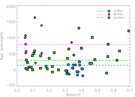
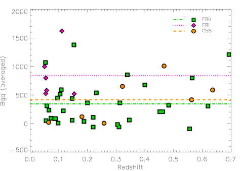
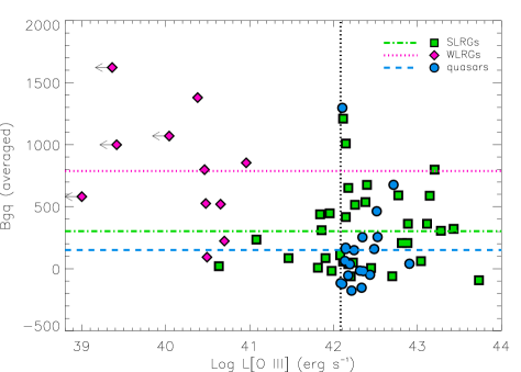
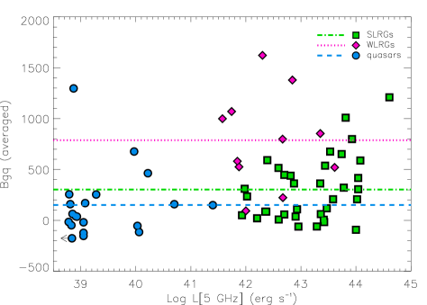
Figure 1: (a) Spatial clustering amplitude versus redshift for the SLRGs, WLRGs and type-2 quasars in the samples considered here. Horizontal lines correspond to the mean B${}_{gq}^{av}$ of each class (dashed line: type-2 quasars, dotted line: WLRGs and dot-dashed line: SLRGs). (b) Same as in Figure 1, but for PRGs only and using their radio classification: FRIs (dotted line), FRIIs (dot-dashed line) and CSS/GPS (dashed line). (c) Same as in Figure 1, but versus [O III]$\lambda$5007 luminosity (in units of $\nu L_{\nu}$). Dotted vertical line indicates Log (10${}^{8.5}L_{\sun}$). (d) Same as in Figure 1 but versus 5 GHz luminosity (in units of $\nu L_{\nu}$).

3.1 Abell classification

To better compare the results of our study of the environment of radio-loud and radio-quiet AGN with the literature, here we provide an estimation of the typical spatial clustering amplitudes for the five Abell richness classes, in the chosen cosmology.

As described by McLure & Dunlop (2001), the correlation between B_gq and Abell class is affected by a large scatter, and thus, there is no rigorous transformation between them. Here we have adopted the linear squeme employed by Yee & López-Cruz (1999) and McLure & Dunlop (2001), in which the different Abell classes are separated by $\Delta B_{gq}$ = 400 Mpc^1.77. We use the same normalization as in McLure & Dunlop (2001), that re-calibrated to our cosmology corresponds to $B_{gq}\sim$400 Mpc^1.77. Therefore, for Abell classes 0, 1, 2, 3, 4 and 5, we have B_gq = 400, 800, 1200, 1600, 2000 and 2400 respectively.

To check the transformation between B_gq and Abell class, we can look at the 2Jy PRGs that are known to be at the centre of galaxy clusters, and see if they have B_gq values $\geq$400 (i.e., Abell class 0 or higher). There are at least four PRGs in clusters, according to the literature:

• PKS 0620-52. A cluster environment for this radio galaxy is supported by the existence of a moderately luminous X-ray halo, for which Trussoni et al. (1999) estimated a 0.5-3.5 keV luminosity of 2.0$\times 10^{44}$ erg s^-1, once transformed to our chosen cosmology.

• PKS 0625-35 was the first ranked member of the cluster A3392 (Trussoni et al., 1999). Siebert et al. (1996) measured a X-ray luminosity of 2.3$\times 10^{44}$ erg s^-1 in the 0.1-2.4 keV band for the extended halo of this source.

• PKS 0915-11 (Hydra A) is situated in the Hydra cluster of galaxies and it is one the most powerful radio sources in the local universe. McNamara et al. (2000) reported the discovery of structure in the central 80 kpc of the cluster X-ray-emitting gas, of 0.5-4.5 keV luminosity 2.2$\times 10^{44}$ erg s^-1. More recently, Wise et al. (2007) claimed the existence of an extensive cavity system, as revealed from a deep Chandra image of the hot plasma.

• PKS 1648+05 (Herc A) is at the centre of a cooling flow cluster of galaxies at z=0.154. The X-ray luminosity of the cluster 2.7$\times 10^{44}$ erg s^-1 in the 0.1-2.4 keV band (Siebert et al., 1999). A recent analysis of Chandra X-ray data showed that the cluster has cavities and a shock front associated with the radio source (Nulsen et al., 2005).

These four galaxies have spatial clustering amplitudes (B${}_{gq}^{av}$) of 999, 526, 798 and 520 respectively, which, according to our calibration, correspond to Abell classes 1 and 0. Thus, in the following, we can consider values of B${}_{gq}^{av}\ga 400$ typical of cluster environments.

3.2 WLRGs versus SLRGs

In Figure 1 we plotted the spatial clustering amplitude (B${}_{gq}^{av}$) versus redshift for the SLRGs (green squares), the WLRGs (pink diamonds) and the type-2 quasars (blue circles). In general, WLRGs are concentrated at lower redshifts and are in denser enviroments than SLRGs and type-2 quasars.

We used the Kolmogorov-Smirnov (KS) test to compare the distributions of B${}_{gq}^{av}$ of the 2Jy WLRGs and SLRGs, shown in the top panels of Figure 2. We found that WLRGs are in richer environments than SLRGs, with mean clustering amplitudes of $\bar{B}_{gq}^{av}(SLRGs)=303\pm 53$ and $\bar{B}_{gq}^{av}(WLRGs)=788\pm 140$, and this difference is significant at the 3$\sigma$ level (see Table 6).

Since the redshift distributions of WLRGs and SLRGs are quite different, we compared the environments of the two groups only considering galaxies at $z<0.2$. By doing this redshift cut, we have 14 SLRGs with mean clustering amplitude $\bar{B}_{gq}^{av}=214\pm 55$ and 10 WLRGs with $\bar{B}_{gq}^{av}=781\pm 155$. As in the case of the comparison done considering the whole redshift range, this difference is significant at the 3$\sigma$ level, based on the KS test.

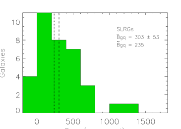
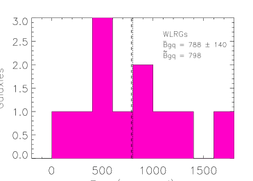
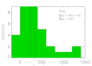
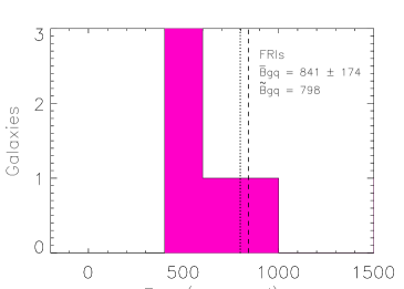
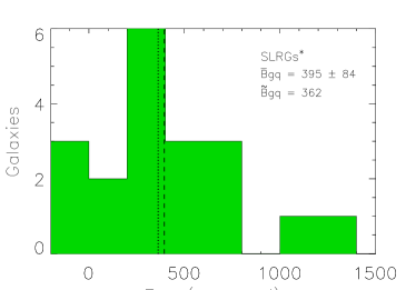
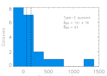
Figure 2: Distribution of spatial clustering amplitudes for the SLRGs and WLRGs (top panels), FRII and FRI radio galaxies (middle panels) and SLRGs* and type-2 quasars (bottom panels). Dotted and dashed lines correspond to the median ($\tilde{B}_{gq}^{av}$) and the average ($\bar{B}_{gq}^{av}$) of the distribution, which are also reported at the top of each panel. Colours are the same as in Figure 1.

Of the 11 WLRGs, all but PKS 0034-01 and PKS 0043-42 have individual B${}_{gq}^{av}$ values characteristic of Abell 0, 1, 2 and 3 clusters, which are larger than the mean value of the whole PRG sample ($\bar{B}_{gq}^{av}=419\pm 60$). According to this, WLRGs constitute a different class of PRGs on the basis of both their spatial clustering amplitude and their optical classification (Tadhunter et al., 1998).

The case of the SLRGs is different. There are only 12 SLRGs with B${}_{gq}^{av}\ga 400$, of which nine have clustering amplitudes characteristic of Abell class 0. The other three SLRGs are PKS 1306-09 and PKS 0117-15 (Abell class 1) and PKS 0409-75 (Abell class 2). Summarising, 82% of the WLRGs in the 2Jy sample are in clusters, according to our definition (B${}_{gq}\ga 400$), compared with only 31% of the SLRGs.

The lack of disturbed morphologies in 73% of the 2Jy WLRGs (Ramos11 RA11), and their large clustering amplitudes, may indicate that at least some WLRGs could be powered by a different triggering mechanism, either cooling flows sinking towards the cluster centers (Tadhunter et al., 1989; Baum et al., 1992; Bremer et al., 1997; Edge et al., 1999, 2010; Best et al., 2005; Sabater et al., 2013) or direct accretion of hot gas from the X-ray haloes (Best et al., 2006; Hardcastle et al., 2007). However, we must be cautious about possible observational selection effects. In particular, it is more difficult to detect tidal features such as shells or broad fans in regions of high galaxy density, since the tidal effects rapidly disrupt these features (see von der Linden et al. 2010 and references therein). Regarding the 27% of 2Jy WLRGs showing the tidal features, it is well below the background rate of interactions measured for the quiescent population of early-type galaxies of same mass and redshift (53%; Ramos12 RA12). Thus, the galaxy interactions occurring in those WLRGs may or may not be linked to the fuelling of the AGN.

3.3 FRIs versus FRIIs

In Figure 1 we show the individual B${}_{gq}^{av}$ values of the 2Jy PRGs plotted against redshift highlighting their classification at radio wavelengths. Green squares correspond to FRIIs (33 objects), pink diamonds to FRIs (6 objects), and orange circles to CSS/GPS sources (7 objects).

The FRIs in the sample have redshifts $z<0.2$ and the majority have larger values of B_gq than FRIIs and CSS/GPS sources. In fact, their mean clustering amplitude (B${}_{gq}^{av}=841\pm 174$) is characteristic of an Abell class 1 cluster. This result is not surprising, considering that all the FRIs in the 2Jy sample are WLRGs. Interestingly, WLRGs (and consequently, FRIs) tend to have large ratios of radio luminosity to AGN power, constituting a first indication that dense environments may boost the radio emission of PRGs (see Section 4.1 for further discussion on this).

In the two central panels of Figure 2, we compare the spatial clustering amplitudes of the FRI and FRII radio galaxies in the 2Jy sample. The distributions, based on the KS test, are different at the 3$\sigma$ level if we consider B${}_{gq}^{av}$ (see Table 6). This is in agreement with the results found by Gendre et al. (2013), based on a sample of $\sim$200 radio galaxies at redshift $z\leq$0.3 (see also Prestage & Peacock 1988, 1989; Zirbel 1997).

Hill & Lilly (1991) studied the cluster environments of a sample of 45 FRII radio galaxies at z$\sim$0.5 and compared them with their low-redshift counterparts. Based on this comparison, Hill & Lilly (1991) claimed that high-redshift PRGs are in richer environments than those at low-redshift. However, looking at Figure 1, we do not observe an enhancement in the clustering amplitude of FRIIs with redshift. In fact, if we divide the FRIIs into a low-redhift sample ($z<0.2$; 16 sources) and high-redshift sample ($0.2\leq z<0.7$; 17 sources), we do not find a significant trend in the environments with redshift: $\bar{B}_{gq}^{av}$($z<0.2$) = 351$\pm$98 and $\bar{B}_{gq}^{av}$($0.2\leq z<0.7$) = 340$\pm$90. A lack of redshift dependence in B_gq was also reported by Wold et al. (2000), based on the comparison of a sample of 21 radio-loud quasars with redshifts $0.5\leq z\leq 0.82$ with other literature samples at lower redshifts. Also McLure & Dunlop (2001) reported no epoch dependence in the environments of radio-loud and radio-quiet powerful AGN out to redshift z=0.5.

Comparison	Targets	$\bar{B}_{gq}$	$\bar{B}_{gq}^{av}$	$\bar{B}_{gq}^{med}$
SLRGs	35	233$\pm$64	303$\pm$53	319$\pm$58
WLRGs	11	759$\pm$156	788$\pm$140	795$\pm$253
KS test	…	98.2%	99.7%	78.6%
FRII	33	284$\pm$75	345$\pm$65	344$\pm$69
FRI	6	811$\pm$230	841$\pm$174	1087$\pm$551
KS test	…	98.8%	99.8%	…
SLRGs*	19	337$\pm$90	395$\pm$84	400$\pm$84
Type-2 quasars	20	184$\pm$87	151$\pm$76	159$\pm$76
KS test	…	83.9%	98.8%	98.8%

Table 6: Comparison between the cluster environments of 1) SLRGs and WLRGs, 2) FRIIs and FRIs, and 3) SLRGs and type-2 quasars with [O III] luminosities larger than 10${}^{8.5}L_{\sun}$. $\bar{B}_{gq}\pm\sigma(B_{gq})/\sqrt{n}$ is reported for each group, with n equal to the number of targets included in the mean, together with the results of the KS test (significance level). We do not report KS test results for the comparison between $B_{gq}^{med}$(FRI) and $B_{gq}^{med}$(FRII) because there are only two FRIs with $B_{gq}^{med}$ available.

3.4 PRGs and type-2 quasars

The type-2 quasars are concentrated around low values of B_gq (see Table 6), with the exceptions of J0904-00, J0320+00 and J0123+00 (B${}_{gq}\ga 400$; i.e. cluster-like). To compare the environments of PRGs and type-2 quasars, it is necessary to consider the same selection criterion used by Bessiere et al. (2012) for the type-2 quasars, and select only PRGs with [O III] luminosities larger than 10${}^{8.5}L_{\sun}$. We did not only consider PRGs with redshits in the same range as the type-2 quasar sample (i.e. $0.3\leq z\leq 0.41$) because that would leave us with five PRGs only, not enough for any statistical comparison. However, we used our $0.2\leq z<0.7$ PRG sample to have a more comparable redshift range. By applying these luminosity and redshift cuts, we ended up with 19 SLRGs (hereafter SLRGs*) whose environments are denser, on average, than those of the 20 type-2 quasars (see bottom panels of Figure 2). The significance of this difference is 98.8% according to the KS test (2$\sigma$; see Table 6). If we further restrict the redshift range (e.g. $0.2\leq z<0.5$) in order to better match that of the type-2 quasars, the difference between environments becomes smaller (93.6%). Thus, although the results presented here hint at a difference between the environments of PRGs and type-2 quasars, larger samples are required to confirm them statistically.

If confirmed for a larger sample, the latter results would be in agreement with the pioneering works of Yee & Green (1984, 1987) and Ellingson et al. (1991). More recently, using a sample of over 2,000 radio-loud AGN selected from SDSS with redshifts 0.03$<$z$<$0.3, Best et al. (2005) claimed that optical AGN and radio-loud AGN are different phenomena and are triggered by different mechanisms. The latter authors claimed that the probability of a galaxy being radio-loud is independent of its classification in the optical. Best et al. (2005) and also Kauffmann et al. (2008), using the same galaxy sample, reported that radio-loud AGN are generally found in denser environments than radio-quiet AGN, coinciding with our results (see also Inskip et al., in preparation for a detailed study of the host galaxy properties of the 2Jy radio galaxies). However, it is worth noting that the radio-loud AGN studied by Best et al. (2005) have much lower radio luminosities (L${}_{1.4GHz}=10^{23}-10^{25}$ W Hz^-1) than the majority of 2Jy radio galaxies.

Similar results were found at higher redshift by Donoso et al. (2010) and Falder et al. (2010), based on samples of radio-loud and radio-quiet AGN at redshift 0.4$<$z$<$0.8 and z$\sim$1 respectively: both found evidence for increasing overdensity with increasing radio luminosity (see also Serber et al. 2006), as well as for radio-loud AGN being in denser environments than radio-quiet galaxies.

On the other hand, McLure & Dunlop (2001) and Wold et al. (2001) found no significant difference between the environments of luminous radio-loud and and radio-quiet type-1 and type-2 quasars at z$\sim$0.2.

If confirmed, the difference between the environments of PRGs and type-2 quasars would not support the hypothesis of luminous AGN cycling between radio-loud and radio-quiet phases within a single quasar triggering event (see e.g. Nipoti et al. 2005). Typically, the radio-loud phase in PRGs is expected to last over a period of $t_{PRG}\sim 100$ Myr (Leahy et al., 1989; Blundell et al., 1999; Shabala et al., 2008), not sufficient for a change in the large scale environment surrounding a typical radio-loud AGN. However, as discussed above, observations of larger samples are required to put these results on a firmer statistical footing.

3.5 Star formation versus environment

Using multi-wavelength data of the 2Jy sample of PRGs, including optical spectroscopy and mid- and far-infrared imaging and spectroscopy, Dicken et al. (2012) searched for recent star formation activity (RSFA) in the host galaxies of the 46 radio sources. The authors used four different diagnostic methods to determine whether or not there is recent star formation present in the 2Jy host galaxies and they confirmed the presence of RSFA in 20% of the sample (i.e. in nine of the 2Jy PRGs). Here we consider that an object has RSFA if it shows evidence for star formation activity based on a minimum of two diagnostic methods. In Ramos11 RA11, we searched for a possible relation between optical morphology and star formation activity, but we did not find any significant difference between the morphologies of the star-forming galaxies and those without recent star formation.

Now we can look at the individual spatial clustering amplitudes of the 2Jy galaxies with and without RSFA. We find that 78% of the galaxies with RSFA (7 of the 9) are in clusters of Abell types 0, 1 and 2. On the other hand, if we look at the clustering amplitudes of the 35 galaxies without RSFA (we discarded the 9 PRGs with confirmed RSFA and another 2 with RSFA confirmed by one diagnostic method only; Dicken et al. 2012), we find 37% in clusters. Thus, in spite of the limited number of PRGs with signs of RSFA, our results show an enhancement of star formation activity in denser environments.

Galaxy interactions could be an explanation for the detection of RSFA in the seven 2Jy PRGs in clusters. The moderate densities of these clusters favour galaxy interactions, and indeed we detect signs of interactions in 6 of them, as indicated in Table 4. These interactions could be leading to an enhancement of the star formation activity in their galaxy hosts. An alternative explanation for the RSFA detected in the 2Jy PRGs in relatively dense environments could be cooling flows taking place at the centers of these galaxy clusters. Searching for cooling gas at the centers of galaxy clusters is very challenging because of the low gas density, and because these flows are much less massive than expected (Fabian, 1994, 2012). AGN feedback has been proposed as the energetic process necessary to balance radiative cooling, preventing massive cooling flows and intense star formation. However, very recently, McDonald et al. (2012) reported the existence of a massive and X-ray luminous cluster at redshift z=0.6 with a cooling rate of 3820 M${}_{\sun}~{}yr^{-1}$. Interestingly, the central galaxy hosts a powerful AGN and a massive starburst, where stars are forming at a rate of 740 M${}_{\sun}~{}yr^{-1}$. McDonald et al. (2012) claimed that this cluster might be an example of a system in which the AGN feedback, which would otherwise suppress the cooling flow, is not completely established.

4 Discussion

In this section we discuss the differences and similarities found among the environments of our complete samples of PRGs, type-2 quasars and quiescent early-type galaxies (EGS and EGS*). To perform those comparisons, we have used the KS non-parametric test for the equality of the one-dimensional distributions of spatial clustering amplitudes. In this regard, the reader should bear in mind that, although we find significant differences between the environments of some of the groups discussed here, there are also substantial overlaps between them (see e.g. Figure 2).

4.1 Dependence of radio power on environment

As first suggested by Barthel & Arnaud (1996) for the case of Cygnus A and a few other sources, the radio luminosity may be affected by the environments of the radio sources (see also Best et al. 2005; Kauffmann et al. 2008; Falder et al. 2010 and references therein). In particular, for a given intrinsic jet power, the radio luminosities of FRII radio galaxies may be boosted in rich environments because of the strong interaction between the relativistic plasma and the hot X-ray emitting gas. Therefore, one would expect that the richer the environment, the higher the radio luminosities for a given intrinsic AGN power. To test this possibility, in Figures 3 and 3 we present B${}_{gq}^{av}$ versus the luminosity ratios L(5 GHz)/L([O III]$\lambda$5007) and L(5 GHz)/L(24 µm) respectively. These ratios tell us how the radio luminosities of PRGs are affected by the environment for a given intrinsic AGN power, as indicated by the [O III] and 24 µm luminosities (Dicken et al., 2009).

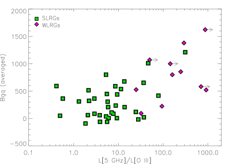
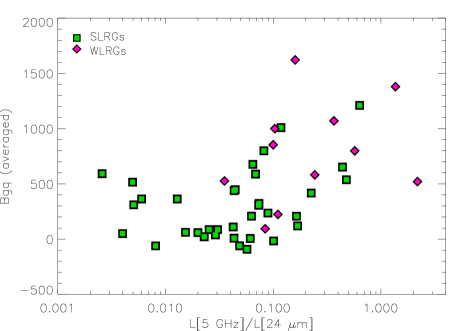
Figure 3: (a) Spatial clustering amplitude versus 5 GHz/[O III]$\lambda$5007 luminosity ratio for SLRGs and WLRGs. (b) Same as in Figure 3 but versus 5 GHz/24 µm. Both ratios have been calculated using luminosities in units of $\nu L_{\nu}$.

From Figures 3 and 3 we see that, below L(5 GHz)/L([O III]$\lambda$5007)$\sim$40 and L(5 GHz)/L(24 µm)$\sim$0.1, there is no clear relationship with B_gq. The majority of SLRGs in the 2Jy sample are included in the previous limits. However, if we look at the sources with the richest environments (B${}_{gq}\ga 800$; Abell class $>$1), they all have relatively large L(5 GHz)/L([O III]$\lambda$5007) and L(5 GHz)/L(24 µm) ratios. Alternatively, all sources with L(5 GHz)/L([O III]$\lambda$5007)$\geq$100 and/or L(5 GHz)/L(24 µm)$\geq$0.3 reside in relatively rich environments (B${}_{gq}\geq 500$) and are WLRGs. The only exceptions are the SLRGs PKS 0409-75 and PKS 1306-09.

Summarising, although we find no clear correlations between the environments of and the emission line luminosities and radio powers (see Figures 1 and 1), we find that the objects with the largest clustering amplitudes –most of which are WLRGs/FRIs– tend to have larger ratios of radio luminosity to intrinsic AGN power. This might be the result of jet interactions with a high density hot gas environment, which would likely favour a more efficient transformation of AGN power into radio luminosity. Alternatively, it could be a consequence of different accretion modes acting in WLRGs (i.e. cooling flows or direct accretion of hot gas), or of the properties of the supermassive black holes (SMBHs) themselves, influenced by the environment. The merger histories of central cluster galaxies may be different from those in the field, leading, for example, to more rapidly spinning black holes (Fanidakis et al., 2011) and to an increased incidence of radio-loud AGN.

4.2 Comparison with control sample of quiescent early-type galaxies

In the previous sections we have discussed the role of environment on the triggering of PRGs and type-2 quasars, but it is necessary to compare these environments with those of the quiescent galaxies in the comparison samples, as we did with the galaxy interactions in Ramos12 RA12 and Bessiere et al. (2012).

In order to do this, first, we compared the environments of PRGs at $0.2\leq z\leq 0.7$ with the parent EGS control sample of 107 early-type galaxies. Second, for the type-2 quasars, we used the 51 early-type galaxies with redshifts $0.3\leq z\leq 0.41$ that comprise the EGS* control sample. In Tables 8 and 9 we report the individual B_gq values that we obtained for the EGS and EGS* samples.

In Table 7 we show the mean values of the distributions of B_gq, B${}_{gq}^{av}$ and B${}_{gq}^{med}$ that we measured for the EGS and EGS* samples, and the comparison with the PRGs and type-2 quasars. First, we find a significant difference between the environments of PRGs and EGS sample (see top panels of Figure 4). PRGs at $0.2\leq z<0.7$ (21 SLRGs and only one WLRG) are, on average, in denser environments ($\bar{B}_{gq}^{av}=384\pm 79$) than their quiescent counterparts ($\bar{B}_{gq}^{av}=111\pm 21$). This difference is significant at the 3$\sigma$ level according to the KS test (see Table 7).

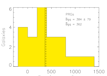
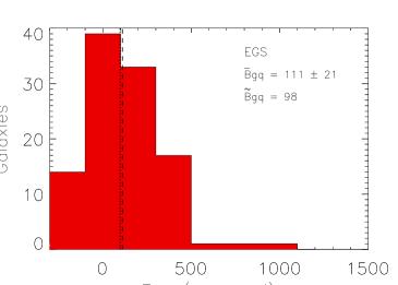
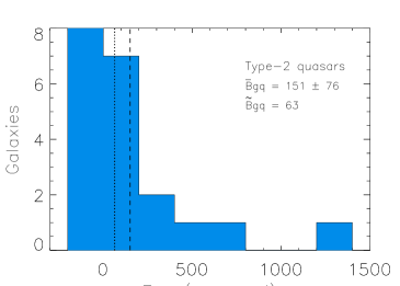
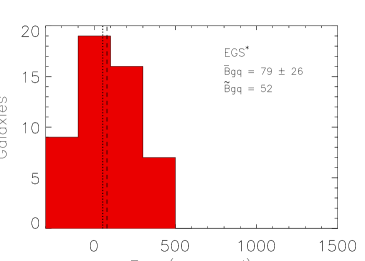
Figure 4: Distribution of spatial clustering amplitudes of the PRGs with redshifts $0.2\leq z<0.7$ and EGS galaxies (top panels) and of the type-2 quasars and EGS* galaxies (bottom panels). Dotted and dashed lines correspond to the median and the average of the distribution respectively. Control sample histograms are represented as red (EGS and EGS*), PRGs as yellow and type-2 quasars as blue.

Although we do not have a control sample suitable for the study of the environment for the low-redshift 2Jy PRGs ($z<0.2$; see Section 2.3), the larger number of WLRGs in it (10 WLRGs and 14 SLRGs), as compared to the high-redshift subsample, increases the mean of B${}_{gq}^{av}$ up to 450$\pm$91. Therefore, it seems logical to assume that PRGs at $z<0.2$ also are in denser environments than quiescent early-type galaxies.

Comparison	Targets	Bgq	B${}_{gq}^{av}$	B${}_{gq}^{med}$
PRGs	22	344$\pm$85	384$\pm$79	389$\pm$79
EGS	107	112$\pm$20	111$\pm$21	101$\pm$21
KS test	…	98.8%	99.7%	99.9%
Type-2 quasars	20	184$\pm$87	151$\pm$76	159$\pm$76
EGS*	51	79$\pm$26	79$\pm$26	77$\pm$25
KS test	…	21.8%	15.5%	40.4%

Table 7: Comparison between the cluster environments of 1) PRGs and whole EGS control sample ($0.2\leq z<0.7$) and 2) type-2 quasars and EGS* control sample ($0.3\leq z\leq 0.41$). $\bar{B}_{gq}\pm\sigma(B_{gq})/\sqrt{n}$ is reported for each group, with n equal to the number of targets included in the mean, together with the results of the KS test (significance level).

The case of the type-2 quasars is different. We do not find a significant difference between the environments of active ($\bar{B}_{gq}^{av}=151\pm 76$) and non-active early-type galaxies ($\bar{B}_{gq}^{av}=79\pm 26$) at redshift $0.3\leq z\leq 0.41$ and M_B=[-22.1,-20.3] mag (see Table 7 and bottom panels of Figure 4).

This result is in apparent contradiction with Serber et al. (2006), who claimed that, on scales ranging from 25 kpc to 1 Mpc, quasars at $z\leq 0.4$ and M_B=[-23.0,-20.8] mag are located in denser environments than their quiescent counterparts. The counting radius that we are using (170 kpc) should be comparable to the small scales considered by Serber et al. (2006), but our analysis has the advantage of considering the galaxies contained in a volume rather than in an area. On the other hand, on larger scales, of $\sim$1 Mpc, Serber et al. (2006) found that quasars inhabit similar environments than the control sample galaxies.

As explained in the Introduction, the periods of black hole growth are coupled with the growth of the host galaxy. Consequently, we do not expect to see a difference in the environment of radio-quiet quasars and quiescent early-type galaxies of the same mass and redshift. The AGN phase represents a very small fraction of the life of a massive galaxy, and the environment will not change significantly within the timespan of a single period of nuclear activity.

In contrast, only some quiescent early-type galaxies have been/may be radio-loud AGN at some point, and the significant difference that we found between their environments and those of the control sample galaxies is noteworthy. It is not clear why only $\sim$10% of the AGN population is radio-loud. The denser environments that we found here for radio-loud AGN, as compared to radio-quiet AGN and control sample galaxies, points out a possible physical explanation behind the radio jet production. The high density hot gas environment characteristic of clusters could be favouring the transformation of AGN power into radio luminosity. Alternatively, the properties of the SMBHs themselves could be influenced by the environment. The merger histories of central cluster galaxies can lead to more rapidly spinning black holes (Fanidakis et al., 2011) and to an increased incidence of radio-loud AGN.

The work presented here provides evidence for the radio-quiet AGN phase being an ubiquitous stage in the evolution of massive early-type galaxies, as well as for the environment to be responsible, to a certain extent, for the radio loudness of AGN. Our findings also support the picture that radio-loud and radio-quiet AGN are independent phenomena.

In order to confirm the influence that the environment has in AGN radio power, it is important to use larger samples of PRGs, as well as to compare with X-ray information about the environment. In the future, we aim to repeat this study for the 3CRR sample of radio galaxies (Laing et al., 1983) and to compare the results found for the environment of the 2Jy PRGs with X-ray data from the XMM-Newton satellite (Mingo et al., in preparation).

5 Conclusions

We have presented the results from a quantitative analysis of the environments of complete samples of PRGs, type-2 quasars and quiescent early-type galaxies. We have also investigated the connection between environment and the triggering mechanisms for nuclear activity in luminous radio-quiet and radio-loud AGN. Our major results are as follows:

• WLRGs in the 2Jy sample are in richer environments ($\bar{B}_{gq}^{av}=788\pm 140$) than SLRGs ($\bar{B}_{gq}^{av}=303\pm 53$). This difference between their B_gq distributions is significant at the 3$\sigma$ level, based on the KS test. We obtain the same result when we compare the environment of FRI and FRII galaxies. WLRGs/FRIs have large ratios of radio luminosity versus AGN power–by definition–, constituting a first indication that dense environments may boost the radio emission of PRGs.

• We do not observe an enhancement in the clustering of FRIIs with redshift. In fact, if we separate low-redhift FRIIs ($z<0.2$; 16 sources) and high-redshift FRIIs ($0.2\leq z<0.7$; 17 sources), we find similar values of the spatial clustering amplitude: $\bar{B}_{gq}^{av}$($z<0.2$) = 351$\pm$98 and $\bar{B}_{gq}^{av}$($0.2\leq z<0.7$) = 340$\pm$90.

• When we compare the environments of type-2 quasars and PRGs in the 2Jy sample with [O III] luminosities larger than 10${}^{8.5}L_{\sun}$, we find that PRGs are more clustered than the type-2 quasars. However, this difference is significant at the 2$\sigma$ level only. A larger sample is required to put it on a firmer statistical footing.

• If we consider the 20% of the 2Jy sample with recent star formation activity detected, we find that 78% of them (7 of the 9) are in clusters of Abell types 0, 1 and 2. Galaxy interactions could be leading to an enhancement of star formation in the galaxy hosts. Alternatively, cooling flows without a completely established AGN feedback could be favouring the formation of new stars.

• We do not find a significant difference between the environments of radio-quiet AGN and non-active early-type galaxies at redshift $0.3\leq z\leq 0.41$ and M_B=[-22.1,-20.3] mag. This is consistent with the quasar phase being a short-lived but ubiquitous stage in the formation of all massive early-type galaxies.

• We find a significant difference (at the 3$\sigma$ level) between the environments of radio-loud AGN at $0.2\leq z<0.7$ ($\bar{B}_{gq}^{av}=384\pm 79$) and their quiescent counterparts ($\bar{B}_{gq}^{av}=111\pm 21$). This supports a physical origin for radio jet production, with high density hot gas environment favouring the transformation of AGN power into radio luminosity, or alternatively, with the environment influencing the properties of the SMBHs themselves.
  

Appendix A Catalogue completeness.

The aim of this work is to compare the environments of PRGs, type-2 quasars and quiescent early-type galaxies and, based on that, discuss the role of environment on the triggering of nuclear activity. For these comparisons to be meaningful, the galaxy counts around each of the targets considered here have to be done to the same relative magnitude limit. Here we have used the criterion $(m_{*}-1)\leq m\leq(m_{*}+2)$ to count galaxies in both the target and the offset fields, and we need to show that the GMOS-S and Suprime-Cam data are deep enough to count galaxies down to the dimmest limit in each case $(m_{*}+2)$.

As discussed in Section 2.3, in Ramos12 RA12 we measured a median surface brightness of $\mu_{V}$=24.2 mag arcsec^-2 for the tidal features detected in the galaxy hosts of the EGS galaxies, and a surface brightness range $22\leq\mu_{V}\leq 26$ mag arcsec^-2. In addition, the seeing of the 4 Suprime-Cam images ranges from FWHM = 0.65″to 0.76″. Thus, the EGS and EGS* data are comparable in depth and resolution to the GMOS-S images employed in the study of PRGs and type-2 quasars. However, especially in the case of the 2Jy sample, the GMOS-S data span a wide range of exposure times (from 250 s to 1500 s) and seeing FWHM (from 0.4″ to 1.15″). Thus, it becomes necessary to demonstrate that those images with large seeing values and/or low exposure times are sufficiently deep to count galaxies down to (m^∗+2).

Figure 5 shows six blank histograms of galaxy counts as a function of apparent magnitude (in the r’ and i’-bands) for the three GMOS-S fields with the lowest exposure times (256, 420 and 720 s) and the three with the worst seeing values (FWHM = 1.00-1.15″). The rest of 2Jy and type-2 quasars were observed with exposure times ranging between $\sim$1000 and 2000 s. We also included the galaxy counts measured in the corresponding offset fields (grey histograms), which were observed immediately after each target field, with exposure times ranging from 800 to 1500 s.

The histograms in Figure 5 show a maximum around 23.5 mag, and a sharp cut at $\sim$25 mag. The same behaviour is shown by the galaxy counts in the four Suprime-Cam EGS fields (see Figure 6). In this case, all the fields were observed with the same exposure time and under similar seeing conditions (1800 s and $\sim$0.70″). The larger galaxy counts are due to the different field sizes (34$\times$27 arcmin² for Suprime-Cam and 5.5$\times$5.5 arcmin² for GMOS-S). Finally, in Figure 7 we show the number of counts measured in the two offset fields with the lowest exposure times and worse seeing FWHMs in the r’ and i’-bands respectively.

The histograms in Figures 5, 6 and 7 were plotted after discarding stars, sources close to image boundaries and with saturated and/or corrupted pixels using the CLASS_-STAR and FLAG SExtractor parameters, as described in Section 2.4. By comparing Figures 5, 6 and 7 it is clear that both the control sample and offset field images are comparable in depth and resolution to the PRG and type-2 quasar images.

The vertical dotted lines in Figure 5 correspond to the (m^∗+2) limit for each target, which basically depends on the galaxy redshift. In Figures 6 and 7, the vertical lines indicate the faintest (m^∗+2) limit in each of the four Subaru fields and among all the target fields respectively. Even for the fields with the worst quality data (i.e. largest seeing FWHMs and lowest exposure times), the (m^∗+2) limits are brighter or equal to the maximum of galaxy count distributions. Note that the last two histograms in Figure 5 correspond to galaxies with the highest redshifts in the 2Jy and type-2 quasar samples (z=0.6 and 0.7 respectively), and thus, with the dimmest (m^∗+2) limit. Therefore, we can confidently compare the clustering amplitudes of PRGs, type-2 quasars and control sample galaxies obtained in this work without running into completeness issues.

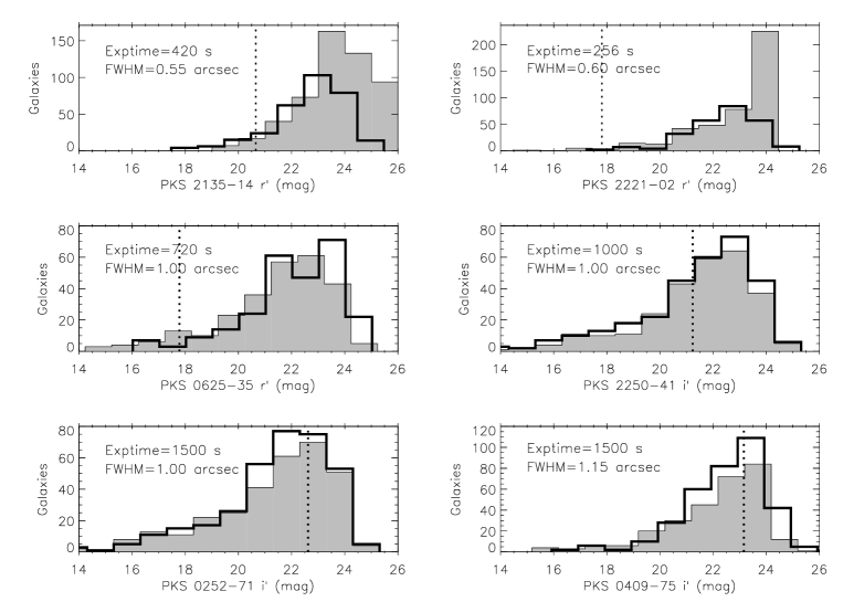
Figure 5: Galaxy counts as a function of apparent magnitude (blank histograms) for the three galaxy fields with the lowest exposure times in the 2Jy and type-2 quasar samples (256, 420 and 720 s) and the three galaxy fields with the worst seeing (FWHM = 1.00-1.15 arcsec). Filled histograms represent the galaxy counts measured in the corresponding offset fields, which were observed immediately after each target field with exposure times between 800 and 1500s. Vertical dotted lines indicate the position of the (m^∗+2) limit used to count galaxies.

Figure 6: Same as in Figure 5, but for the four Suprime-Cam/Subaru fields from which the EGS and EGS* control sample galaxies were taken from. Vertical dotted lines indicate the position of the faintest (m^∗+2) limit used to count galaxies in each field.

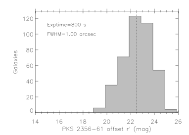
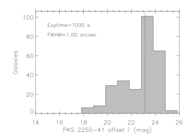
Figure 7: Galaxy counts as a function of apparent magnitude for the two offset fields with the lowest exposure times and worse seeing FWHMs in the r’ and i’-bands respectively. Vertical dotted lines indicate the position of the faintest (m^∗+2) limits among all the targets considered in this work.

Appendix B Galaxy counts and luminosity function normalization.

As described in Section 2.6, the clustering amplitudes discussed in this work depend on the chosen luminosity function. To demonstrate that the luminosity function parameters given in Table 3 are consistent with our background counts, we integrated our evolving luminosity function along the line of sight considering the five redshift bins indicated in Table 3. The predicted background counts as a function of apparent magnitude in the GMOS-S r’ and i’-band filters and in the Suprime-Cam Rc filter are shown as solid lines in the three panels of Figure 8. Using our galaxy catalogs, we counted galaxies after getting rid of stars and sources close to image boundaries, or with saturated and/or corrupted pixels (using the CLASS_-STAR and FLAG SExtractor parameters as described in Section 2.4). We computed the average background counts in the 52 GMOS-S r’-band offset fields, in the 11 i’-band offset fields, and in the four Suprime-Cam Rc images (black dots in Figure 8). We calculated Poissonian errors multiplied by a 1.3 factor to approximate possible departures from Poisson statistics (Yee & López-Cruz, 1999; Wold et al., 2000).

Figure 8: Background counts, represented as black dots, measured from the GMOS-S r’ and i’-band offset fields (left and central panels) and in the four Suprime-Cam Rc images (right panel). Solid lines are the predicted background counts, obtained from integrating the evolving luminosity function along the line of sight considering the five redshift bins indicated in Table 3.

Figure 8 shows that our choice of evolving luminosity function is consistent with the data. The agreement between the predicted and measured number counts and the faint end, up to a limit of 23-24 mag, backs up the results of Appendix A.

In the case of the Rc and r’-band fields (left and right panels of Figure 8), we detect an excess in the number of background counts at magnitudes brighter than 19. After visual inspection of the individual images, we found out that this excess is due to intruder stars that have not been removed from our catalogues. For example, among the 52 r’-band fields, there are 33 sources with $0.7\leq STAR\leq 0.85$ and r’$\leq$19 mag which are either stars with small deviations from symmetry produced by extremelly faint galaxies next to them, or stars immersed in the bright haloes of saturated stars. These 33 sources are distributed in 8 out of the 52 GMOS-S r’-band fields. This explains the lack of bright excess in the i’-band counts (central panel of Figure 8), which were measured in 11 offset fields only. In the Rc-band Suprime-Cam fields we see the same effect as in the GMOS-S r’-band, because we are measuring galaxy counts in an even larger area ($\sim$1 deg²).

Appendix C Clustering amplitudes of control sample galaxies.

Here we present the individual spatial clustering amplitudes of the 107 early-type galaxies in the EGS sample (Table 8) and 51 early-type galaxies in the EGS* sample (Table 9).

irac ID	zPHOT	Nt	Nb	Bgq	N${}_{b}^{av}$	$\sigma$	B${}_{gq}^{av}\pm\Delta B_{gq}^{av}$	N${}_{b}^{med}$	B${}_{gq}^{med}$	Morphology
(1)	(2)	(3)	(4)	(5)	(6)	(7)	(8)	(9)	(10)	(11)
004162	0.48	5	1.97	351	2.08	0.13	338$\pm$294	2.18	326	…
006612	0.31	6	1.30	447	1.42	0.08	436$\pm$252	1.45	433	B,F,[D],[T
006613	0.30	6	1.26	446	1.37	0.08	436$\pm$248	1.42	431	B
056690-1	0.50	4	2.32	199	2.17	0.15	217$\pm$278	2.27	205	[A],[B]
060191	0.57	5	2.60	307	2.46	0.21	324$\pm$330	2.60	307	F
060958	0.40	3	1.75	132	1.74	0.08	133$\pm$216	1.75	132	T,[A],[B]
061249	0.65	4	3.10	125	2.88	0.32	154$\pm$336	3.10	125	[T]
066105	0.51	4	2.31	202	2.20	0.16	215$\pm$281	2.31	202	[A]
067417	0.39	0	1.71	-178	1.71	0.07	-178$\pm$113	1.71	-178	…
072533	0.33	1	1.49	-47	1.49	0.07	-47$\pm$137	1.49	-48	S
073519	0.49	0	2.21	-259	2.11	0.14	-247$\pm$141	2.21	-259	[A]
074777	0.42	6	1.86	449	1.82	0.07	453$\pm$292	1.86	449	[S]
074924	0.41	5	1.79	344	1.77	0.07	345$\pm$266	1.79	344	…
077695	0.35	1	1.58	-58	1.57	0.08	-57$\pm$144	1.58	-58	T
079968	0.60	5	2.80	290	2.62	0.25	313$\pm$343	2.80	290	F
082325	0.55	2	2.51	-63	2.38	0.20	-47$\pm$236	2.51	-63	[F]
083714	0.50	5	2.27	323	2.17	0.15	335$\pm$302	2.27	323	F
088031	0.50	4	2.03	233	2.17	0.15	217$\pm$278	2.27	205	F
090430	0.38	3	1.67	137	1.68	0.07	137$\pm$212	1.69	136	A,F,[B]
092065	0.55	3	2.19	101	2.38	0.20	78$\pm$271	2.51	61	B
092765	0.35	2	1.55	44	1.57	0.08	42$\pm$172	1.58	41	[A],[T]
093764-1	0.39	2	1.70	31	1.71	0.07	30$\pm$184	1.71	30	[S]
094231	0.41	2	1.75	27	1.77	0.07	24$\pm$187	1.79	22	2F,[T]
094966	0.46	1	1.91	-103	2.00	0.11	-113$\pm$174	2.09	-123	2T
095727	0.38	3	1.67	137	1.68	0.07	137$\pm$212	1.69	136	F,S
099954	0.27	1	1.33	-29	1.27	0.10	-24$\pm$122	1.33	-29	[T]
102757	0.22	3	1.27	147	1.19	0.09	154$\pm$166	1.21	152	2S
102982	0.60	4	2.42	208	2.62	0.25	181$\pm$316	2.80	158	F
103198	0.38	1	1.67	-69	1.68	0.07	-70$\pm$151	1.69	-71	2N,F,S
104038	0.46	4	1.91	236	2.00	0.11	226$\pm$262	2.09	216	B
104729	0.63	1	2.52	-207	2.77	0.29	-241$\pm$232	2.97	-268	A
105193	0.23	2	1.26	63	1.19	0.08	69$\pm$143	1.23	66	[S]
106324	0.26	3	1.33	149	1.25	0.10	156$\pm$175	1.33	149	[T]
106984	0.45	3	1.88	125	1.95	0.10	117$\pm$232	2.02	110	A,[I]
111427	0.32	2	1.47	51	1.45	0.09	52$\pm$164	1.47	51	2N,T,2I
112580	0.51	4	2.06	232	2.20	0.16	215$\pm$281	2.31	202	[B]
113088	0.48	3	1.97	119	2.08	0.13	106$\pm$243	2.18	94	[B]
113577	0.67	2	2.73	-102	3.01	0.35	-143$\pm$286	3.24	-176	[A]
114966	0.61	7	2.45	606	2.67	0.27	578$\pm$397	2.84	554	2T,S
115327	0.35	2	1.55	44	1.57	0.08	42$\pm$172	1.58	41	2F,[T]
115594	0.31	2	1.45	52	1.42	0.08	55$\pm$164	1.45	52	2N,T
118942	0.37	1	1.64	-65	1.63	0.06	-64$\pm$148	1.65	-66	…
119696	0.50	2	2.03	-3	2.17	0.15	-19$\pm$209	2.27	-32	B,F
122098	0.22	0	1.27	-108	1.19	0.09	-101$\pm$77	1.21	-102	…
124509	0.34	4	1.52	244	1.52	0.07	244$\pm$221	1.53	243	B,2T,F
125663	0.53	2	2.13	-15	2.29	0.18	-35$\pm$228	2.41	-50	[F]
126918-1	0.49	4	2.00	234	2.11	0.14	221$\pm$273	2.21	209	F,[B]
127241	0.59	4	2.36	213	2.56	0.24	187$\pm$312	2.73	165	…
127457	0.50	2	2.03	-3	2.17	0.15	-19$\pm$209	2.27	-32	2N,A
128074	0.34	4	1.52	244	1.52	0.07	244$\pm$221	1.53	243	B,[F]
128416	0.58	6	2.33	474	2.52	0.23	449$\pm$359	2.67	430	…
132682	0.33	1	1.40	-39	1.49	0.07	-47$\pm$137	1.49	-48	…
135859	0.40	2	1.66	36	1.74	0.08	27$\pm$186	1.75	26	[I]

irac ID	zPHOT	Nt	Nb	Bgq	N${}_{b}^{av}$	$\sigma$	B${}_{gq}^{av}\pm\Delta B_{gq}^{av}$	N${}_{b}^{med}$	B${}_{gq}^{med}$	Morphology
(1)	(2)	(3)	(4)	(5)	(6)	(7)	(8)	(9)	(10)	(11)
138794	0.50	3	2.05	113	2.17	0.15	98$\pm$250	2.27	86	[T]
139190	0.44	0	1.82	-201	1.91	0.09	-211$\pm$127	1.97	-218	…
140456	0.30	5	1.26	352	1.37	0.08	342$\pm$230	1.42	336	2T
140758	0.43	1	1.78	-85	1.87	0.08	-94$\pm$164	1.92	-101	S
141714	0.44	4	1.82	242	1.91	0.09	232$\pm$256	1.97	225	[B],[S]
143149	0.37	3	1.55	148	1.63	0.06	139$\pm$206	1.65	138	T
143536	0.50	1	2.05	-123	2.17	0.15	-138$\pm$186	2.27	-150	[T]
145098	0.32	3	1.35	159	1.45	0.09	149$\pm$192	1.47	147	A,T
145434	0.48	2	1.96	4	2.08	0.13	-9$\pm$209	2.18	-21	4T
146298	0.59	2	2.34	-45	2.56	0.24	-73$\pm$253	2.73	-95	[A]
152722	0.49	2	1.99	1	2.11	0.14	-13$\pm$220	2.21	-25	[F]
156161	0.30	3	1.26	164	1.37	0.08	153$\pm$186	1.42	148	T
157751	0.47	2	1.94	6	2.05	0.12	-5$\pm$185	2.14	-16	…
157878	0.46	3	1.90	125	2.00	0.11	113$\pm$236	2.09	103	F
159123	0.56	0	2.27	-286	2.43	0.21	-307$\pm$164	2.56	-324	T
159936	0.41	1	1.70	-75	1.77	0.07	-83$\pm$161	1.79	-84	2N
160442	0.47	5	1.94	350	2.05	0.12	338$\pm$290	2.14	327	B,A
160500	0.34	5	1.43	352	1.52	0.07	343$\pm$242	1.53	342	B,2T
161724	0.34	4	1.43	253	1.52	0.07	244$\pm$221	1.53	243	[F]
165265	0.67	4	2.69	185	3.01	0.35	140$\pm$349	3.24	107	B,T
166730	0.36	1	1.51	-51	1.60	0.07	-61$\pm$147	1.62	-62	S,T
169386	0.47	0	1.94	-222	2.05	0.12	-234$\pm$136	2.14	-245	…
172474	0.51	2	2.07	-8	2.20	0.16	-24$\pm$225	2.31	-37	T,B,F
173901	0.32	0	1.35	-129	1.45	0.09	-140$\pm$97	1.47	-141	…
175347	0.60	1	2.39	-184	2.62	0.25	-214$\pm$221	2.80	-236	S,[B]
175590	0.56	1	2.65	-209	2.43	0.21	-180$\pm$206	2.56	-197	[A]
177990	0.25	1	1.11	-9	1.23	0.10	-20$\pm$118	1.30	-26	F,[2N]
178118	0.46	5	2.11	328	2.00	0.11	340$\pm$286	2.09	330	…
178724	0.52	3	2.43	69	2.25	0.17	91$\pm$259	2.36	77	A
178868	0.37	4	1.70	235	1.63	0.06	242$\pm$231	1.65	240	F
180420	0.54	9	2.54	800	2.33	0.19	825$\pm$403	2.46	809	2N,2T,[B]
181402	0.38	6	1.75	439	1.68	0.07	447$\pm$277	1.69	446	[I],[A]
181444	0.31	1	1.50	-47	1.42	0.08	-39$\pm$131	1.45	-42	2S,[I]
181736	0.46	6	2.11	441	2.00	0.11	453$\pm$308	2.09	443	…
181914	0.36	0	1.69	-170	1.60	0.07	-162$\pm$106	1.62	-163	…
182762	0.43	4	1.94	226	1.87	0.08	234$\pm$253	1.92	227	[F]
183081	0.36	6	1.69	436	1.60	0.07	444$\pm$269	1.62	443	F,[T]
183836	0.44	3	2.00	111	1.91	0.09	121$\pm$231	1.97	114	[S]
184041	0.53	4	2.48	186	2.29	0.18	209$\pm$289	2.41	194	F,S
184315	0.50	3	2.32	80	2.17	0.15	98$\pm$250	2.27	86	2N
186058	0.54	3	2.54	57	2.33	0.19	82$\pm$263	2.46	66	[A]
189727	0.64	4	3.15	116	2.83	0.31	161$\pm$336	3.03	133	…
190795	0.51	4	2.37	195	2.20	0.16	215$\pm$281	2.31	202	T,S
193464	0.42	3	1.90	119	1.82	0.07	128$\pm$224	1.86	124	2N,F
193507	0.47	1	2.16	899	2.05	0.12	912$\pm$388	2.14	901	2N,[B]
193737	0.50	2	2.32	-37	2.17	0.15	-19$\pm$209	2.27	-32	…
193974	0.40	2	1.84	17	1.74	0.08	27$\pm$186	1.75	26	[S]
194092	0.51	5	2.37	314	2.20	0.16	335$\pm$305	2.31	321	[T]
196827	0.37	4	1.70	235	1.63	0.06	242$\pm$231	1.65	240	T
198295	0.54	2	2.54	-66	2.33	0.19	-41$\pm$236	2.46	-57	[S]
199503	0.50	1	2.32	-156	2.17	0.15	-138$\pm$186	2.27	-150	T
202111	0.27	1	1.37	-33	1.27	0.10	-24$\pm$122	1.33	-29	[S]
204161	0.62	2	3.01	-136	2.72	0.28	-97$\pm$265	2.92	-123	A,[B]
204944	0.28	2	1.39	55	1.31	0.09	63$\pm$156	1.36	58	T,S

Table 8: Same as in Table 4 but for the 107 early-type galaxies in the EGS sample. Last column corresponds to the morphological classification in Ramos12 RA12: T: Tail; F: Fan; B: Bridge; S: Shell; D: Dust feature; 2N: Double Nucleus; 3N: Triple Nucleus; A: Amorphous Halo; I: Irregular feature; and J: Jet. Brackets indicate uncertain identification of the feature.

irac ID	zPHOT	Ng	Nb	Bgq	N${}_{b}^{av}$	$\sigma$	B${}_{gq}^{av}\pm\Delta B_{gq}^{av}$	N${}_{b}^{med}$	B${}_{gq}^{med}$	Morphology
(1)	(2)	(3)	(4)	(5)	(6)	(7)	(8)	(9)	(10)	(11)
006612	0.31	6	1.30	447	1.42	0.08	436$\pm$252	1.45	433	B,F,[D],[T
006613	0.30	6	1.26	446	1.37	0.08	436$\pm$248	1.42	431	B
060958	0.40	3	1.75	132	1.74	0.08	133$\pm$216	1.75	132	T,[A],[B]
066504	0.39	0	1.71	-178	1.71	0.07	-178$\pm$113	1.71	-178	…
067417	0.39	1	1.49	-47	1.49	0.07	-47$\pm$137	1.49	-48	…
069266	0.35	5	1.79	344	1.77	0.07	345$\pm$266	1.79	344	…
072533	0.33	1	1.58	-58	1.57	0.08	-57$\pm$144	1.58	-58	S
073242	0.41	3	1.67	137	1.68	0.07	137$\pm$212	1.69	136	…
074924	0.41	2	1.55	44	1.57	0.08	42$\pm$172	1.58	41	…
077695	0.35	2	1.70	31	1.71	0.07	30$\pm$184	1.71	30	T
090430	0.38	2	1.75	27	1.77	0.07	24$\pm$187	1.79	22	A,F,[B]
092765	0.35	3	1.67	137	1.68	0.07	137$\pm$212	1.69	136	[A],[T]
093764-1	0.39	1	1.67	-69	1.68	0.07	-70$\pm$151	1.69	-71	[S]
094231	0.41	2	1.47	51	1.45	0.09	52$\pm$164	1.47	51	2F,[T]
095727	0.38	2	1.55	44	1.57	0.08	42$\pm$172	1.58	41	F,S
096307	0.34	2	1.45	52	1.42	0.08	55$\pm$164	1.45	52	I
103198	0.38	1	1.64	-65	1.63	0.06	-64$\pm$148	1.65	-66	2N,F,S
111427	0.32	4	1.52	244	1.52	0.07	244$\pm$221	1.53	243	2N,T,2I
115327	0.35	4	1.52	244	1.52	0.07	244$\pm$221	1.53	243	2F,[T]
115594	0.31	1	1.40	-39	1.49	0.07	-47$\pm$137	1.49	-48	2N,T
118942	0.37	2	1.66	36	1.74	0.08	27$\pm$186	1.75	26	…
124509	0.34	5	1.26	352	1.37	0.08	342$\pm$230	1.42	336	B,2T,F
128074	0.34	3	1.55	148	1.63	0.06	139$\pm$206	1.65	138	B,[F]
132682	0.33	3	1.35	159	1.45	0.09	149$\pm$192	1.47	147	…
135859	0.40	3	1.26	164	1.37	0.08	153$\pm$186	1.42	148	[I]
136904	0.39	1	1.70	-75	1.77	0.07	-83$\pm$161	1.79	-84	…
140456	0.30	5	1.43	352	1.52	0.07	343$\pm$242	1.53	342	2T
143149	0.37	4	1.43	253	1.52	0.07	244$\pm$221	1.53	243	T
145098	0.32	1	1.51	-51	1.60	0.07	-61$\pm$147	1.62	-62	A,T
147147	0.38	0	1.35	-129	1.45	0.09	-140$\pm$97	1.47	-141	[T]
156161	0.30	4	1.70	235	1.63	0.06	242$\pm$231	1.65	240	T
159936	0.41	6	1.75	439	1.68	0.07	447$\pm$277	1.69	446	2N
160500	0.34	1	1.50	-47	1.42	0.08	-39$\pm$131	1.45	-42	B,2T
161724	0.34	0	1.69	-170	1.60	0.07	-162$\pm$106	1.62	-163	[F]
166730	0.36	6	1.69	436	1.60	0.07	444$\pm$269	1.62	443	S,T
173901	0.32	2	1.84	17	1.74	0.08	27$\pm$186	1.75	26	…
174667	0.34	4	1.70	235	1.63	0.06	242$\pm$231	1.65	240	[A]
178868	0.37	0	1.75	-181	1.68	0.07	-173$\pm$111	1.69	-174	F
181402	0.38	3	1.50	142	1.42	0.08	150$\pm$189	1.45	147	[I],[A]
181444	0.31	3	1.86	122	1.77	0.07	131$\pm$219	1.79	129	2S,[I]
181914	0.36	0	1.43	-141	1.52	0.07	-150$\pm$101	1.53	-150	…
183081	0.36	2	1.63	39	1.71	0.07	30$\pm$184	1.71	30	F,[T]
184541	0.31	3	1.52	145	1.52	0.07	145$\pm$197	1.53	145	T
186114	0.41	1	1.79	-84	1.77	0.07	-83$\pm$161	1.79	-84	T
193735	0.37	0	1.58	-158	1.57	0.08	-157$\pm$104	1.58	-158	T
193974	0.40	0	1.71	-178	1.71	0.07	-178$\pm$113	1.71	-178	[S]
196827	0.37	4	1.55	235	1.45	0.09	245$\pm$215	1.47	244	T
198078	0.41	0	1.70	-173	1.63	0.06	-167$\pm$109	1.65	-168	[T]
198996	0.32	3	1.86	122	1.77	0.07	131$\pm$219	1.79	129	…
203581	0.32	2	1.55	42	1.45	0.09	52$\pm$164	1.47	51	[T]
207306	0.38	0	1.59	-165	1.68	0.07	-173$\pm$111	1.69	-174	…

Table 9: Same as in Table 4 but for the 51 early-type galaxies in the EGS* sample.

References

- Alexander & Hickox (2012) Alexander, D. M., Hickox, R. C. 2012, NewAR, 56, 93
- Allen et al. (2006) Allen, S. W., Dunn, R. J. H., Fabian, A. C., Taylor, G. B., Reynolds, C. S. 2006, MNRAS, 372, 21
- Bahcall et al. (1997) Bahcall, J. N., Kirhakos, S., Saxe, D. H., Schneider, D. P. 1997, ApJ, 479, 642
- Balmaverde et al. (2008) Balmaverde, B., Baldi, R. D., Capetti, A. 2008, A&A, 486, 119
- Barro et al. (2011) Barro, G., et al. 2011, ApJS, 193, 13
- Barro et al. (2009) Barro, G., et al. 2009, A&A, 494, 63
- Barthel & Arnaud (1996) Barthel, P. D., Arnaud, K. A. 1996, MNRAS, 283, L45
- Baum et al. (1992) Baum S. A., Heckman T., van Breugel W., 1992, ApJ, 398, 208
- Bessiere et al. (2012) Bessiere, P. S., Tadhunter, C. N., Ramos Almeida, C., Villar-Martín, M. 2012, MNRAS, 426, 276
- Bennert et al. (2008) Bennert, N., Canalizo, G., Jungwiert, B., Stockton, A., Schweizer, F., Peng, C. Y., Lacy, M. 2008, ApJ, 677, 846
- Bertin & Arnouts (1996) Bertin, E., Arnouts, S. 1996, A&AS, 117, 393
- Best et al. (2006) Best, P. N., Kaiser, C. R., Heckman, T. M., Kauffmann, G. 2006, MNRAS, 368, L67
- Best et al. (2005) Best, P. N., Kauffmann, G., Heckman, T. M., Brinchmann, J., Charlot, S., Ivezić, Z., White, D. M. 2005, MNRAS, 362, 25
- Blanton (2006) Blanton, M. R. 2006, ApJ, 648, 268
- Blundell et al. (1999) Blundell, K. M., Rawlings, S., Willott, C. J. 1999, AJ, 117, 677
- Bremer et al. (1997) Bremer M. N., Fabian A. C., Crawford C. S., 1997, MNRAS, 284, 213
- Bundy et al. (2010) Bundy, K., et al. 2010, ApJ, 719, 1969
- Buttiglione et al. (2010) Buttiglione, S., Capetti, A., Celotti, A., Axon, D. J., Chiaberge, M. Macchetto, F. D., Sparks, W. B. 2010, A&A, 509, 6
- Canalizo & Stockton (2000) Canalizo, G., Stockton, A. 2000, ApJ, 528, 201
- Canalizo et al. (2007) Canalizo, G., Bennert, N., Jungwiert, B., Stockton, A., Schweizer, F., Lacy, M., Peng, C. 2007, ApJ, 669, 801
- Canalizo & Stockton (2001) Canalizo, G., Stockton, A. 2001, ApJ, 555, 719
- Cole et al. (2000) Cole, S., Lacey, C., Baugh, C. M., Frenk, C. S. 2000, MNRAS, 319, 168
- Cox et al. (2008) Cox, T. J., Jonsson, P., Somerville, R. S., Primack, J. R., Dekel, A. 2008, MNRAS, 384, 386
- Cox et al. (2006) Cox, T. J., Jonsson, P., Primack, J. R., Somerville, R. S. 2006, MNRAS, 373, 1013
- Croton et al. (2006) Croton, D. J., et al. 2006, MNRAS, 365, 11
- Dicken et al. (2008) Dicken, D., Tadhunter, C., Morganti, R., Buchanan, C., Oosterloo, T., Axon, D. 2008, ApJ, 678, 712
- Dicken et al. (2009) Dicken, D., Tadhunter, C., Axon, D., Morganti, R., Inskip, K. J., Holt, J., González Delgado, R., Groves, B. 2009, ApJ, 694, 268
- Dicken et al. (2012) Dicken, D., et al. 2012, ApJ, 745, 172
- Di Matteo et al. (2007) di Matteo, P., Combes, F., Melchior, A.-L., Semelin, B. 2007, A&A, 468, 61
- Di Matteo et al. (2005) Di Matteo, T., Springel, V., Hernquist, L. 2005, Nature, 433, 604
- Donoso et al. (2010) Donoso, E., Li, C., Kauffmann, G., Best, P. N., Heckman, T. M. 2010, MNRAS, 407, 1078
- Dunlop et al. (2003) Dunlop, J. S., McLure, R. J., Kukula, M. J., Baum, S. A., O’Dea, C. P., Hughes, D. H. 2003, MNRAS, 340, 1095
- Edge et al. (2010) Edge, A. C., Oonk, J. B. R., Mittal, R., et al. 2010, A&A, 518, L47
- Edge et al. (1999) Edge, A. C., Ivison, R. J., Smail, Ian, Blain, A. W., Kneib, J.-P. 1999, MNRAS, 306, 599
- Ellingson et al. (1991) Ellingson, E., Yee, H. K. C., Green, R. F. 1991, ApJ, 371, 49
- Ellison et al. (2011) Ellison S. L., Patton D. R., Trevor Mendel J., Scudder J. M., 2011, MNRAS, 418, 2043
- Faber et al. (2007) Faber, S. M., et al. 2007, ApJ, 665, 265
- Fabian (1994) Fabian, A. C. 1994, ARA&A, 32, 277
- Fabian (2012) Fabian, A. C. 2012, ARA&A, 50, 455
- Fadda et al. (2004) Fadda, D., Jannuzi, B. T., Ford, A., Storrie-Lombardi, L. J. 2004, AJ, 128, 1
- Falder et al. (2010) Falder, J. T., et al. 2010, MNRAS, 405, 347
- Fanidakis et al. (2011) Fanidakis, N., Baugh, C. M., Benson, A. J., Bower, R. G., Cole, S., Done, C., Frenk, C. S. 2011, MNRAS, 410, 53
- Fisher et al. (1996) Fisher, K. B., Bahcall, J. N., Kirhakos, S., Schneider, D. P. 1996, ApJ, 468, 469
- Fukugita et al. (1995) Fukugita, M., Shimasaku, K., Ichikawa, T. 1995, PASP, 107, 945
- Gabor et al. (2009) Gabor, J. M., et al. 2009, ApJ, 691, 705
- Gendre et al. (2013) Gendre, M. A., Best, P. N., Wall, J. V., Ker, L. M. 2013, MNRAS, 430, 3086
- Georgakakis et al. (2009) Georgakakis, A., et al. 2009, MNRAS, 397, 623
- Grogin et al. (2005) Grogin, N. A., et al. 2005, ApJ, 627, L97
- Groth et al. (1994) Groth, E. J., et al. 1994, BAAS, 26, 1403
- Groth & Peebles (1977) Groth, E. J., Peebles, P. J. E. 1977, ApJ, 217, 385
- Hardcastle et al. (2007) Hardcastle, M. J., Evans, D. A., Croston, J. H. 2007, MNRAS, 376, 1849
- Heckman et al. (1986) Heckman, T. M., Smith, E. P., Baum, S. A., van Breugel, W. J. M., Miley, G. K., Illingworth, G. D., Bothun, G. D., Balick, B. 1986, ApJ, 311, 526
- Hill & Lilly (1991) Hill, G. J., Lilly, S. J. 1991, ApJ, 367, 1
- Hook et al. (2004) Hook I., Jørgensen I., Allington-Smith J. R., Davies R. L., Metcalfe N., Murowinski R. G., Crampton D. 2004, PASP, 116, 425
- Hopkins et al. (2008a) Hopkins, P. F., Cox, T. J., Kereš, D., Hernquist, L. 2008a, ApJs, 175, 390
- Hopkins et al. (2008b) Hopkins, P. F., Hernquist, L., Cox, T. J., Kereš, D. 2008b, ApJs, 175, 356
- Hutchings (1987) Hutchings, J. B. 1987, ApJ, 320, 122
- Inskip et al. (2010) Inskip, K. J., Tadhunter, C. N., Morganti, R., Holt, J., Ramos Almeida, C., Dicken, D. 2010, MNRAS, 407, 1739
- Jogee (2006) Jogee, S. 2006, in Lecture Notes in Physics, Berlin Springer Verlag, vol. 693, 143
- Kauffmann et al. (1993) Kauffmann, G., White, S. D. M., Guiderdoni, B. 1993, MNRAS, 264, 201
- Kauffmann & Haehnelt (2000) Kauffmann, G., Haehnelt, M. 2000, MNRAS, 311, 576
- Kauffmann et al. (2008) Kauffmann, G., Heckman, T. M., Best, P. N. 2008, MNRAS, 384, 953
- Keel et al. (1996) Keel, W. C. 1996, AJ, 111, 696
- Kron (1980) Kron, R. G. 1980, ApJS, 43, 305
- Kuo et al. (2008) Kuo, C.-Y., Lim, J., Tang, Y.-W., Ho, P. T. P. 2008, ApJ, 679, 1047
- Laing et al. (1983) Laing, R. A., Riley, J. M., Longair, M. S. 1983, MNRAS, 204, 151
- Leahy et al. (1989) Leahy, J. P., Muxlow, T. W. B., Stephens, P. W. 1989, MNRAS, 239, 401
- Longair & Seldner (1979) Longair, M. S., Seldner, M. 1979, MNRAS, 189, 433
- Malkan et al. (1998) Malkan, M. A., Gorjian, V., Tam, R. 1998, ApJ, 117, 25
- McDonald et al. (2012) McDonald, M., et al. 2012, Nature, 488, 349
- McDonald et al. (2011) McDonald, M., Veilleux, S., Mushotzky, R. 2011, ApJ, 731, 33
- McLure & Dunlop (2001) McLure, R. J., Dunlop, J. S. 2001, MNRAS, 321, 515
- McNamara et al. (2000) McNamara, B. R., et al. 2000, ApJ, 534, L135
- Miyazaki et al. (2007) Miyazaki, S., Satoshi, H., Takashi, E., Richard S., Kashikawa, N., Massey, R. J., Taylor, J., Refregier, A. 2007, ApJ, 669, 714
- Miyazaki et al. (2002) Miyazaki, S., et al. 2002, PASJ, 54, 833
- Nipoti et al. (2005) Nipoti, C., Blundell, K. M., Binney, J. 2005, MNRAS, 361, 633
- Nulsen et al. (2005) Nulsen, P. E. J., Hambrick, D. C., McNamara, B. R., Rafferty, D., Birzan, L., Wise, M. W., David, L. P. 2005, ApJ, 625, L9
- Pérez-González et al. (2008) Pérez-González, P. G., Trujillo, I., Barro, G., Gallego, J., Zamorano, J., Conselice, C. J. 2008, ApJ, 687, 50
- Prestage & Peacock (1989) Prestage, R. M., Peacock, J. A. 1989, MNRAS, 236, 959
- Prestage & Peacock (1988) Prestage, R. M., Peacock, J. A. 1988, MNRAS, 230, 131
- (81) Ramos Almeida, C., et al. 2012, MNRAS, 419, 687
- (82) Ramos Almeida, C., Tadhunter, C. N., Inskip, K. J., Morganti, R., Holt, J., Dicken, D. 2011a, MNRAS, 410, 1550
- Ramos Almeida et al. (2011b) Ramos Almeida, C., Dicken, D., Tadhunter, C., Asensio Ramos, A., Inskip, K. J., Hardcastle, M. J., Mingo, B. 2011b, MNRAS, 413, 2358
- Ryan & De Robertis (2010) Ryan, C. J., De Robertis, M. M. 2010, ApJ, 710, 783
- Sabater et al. (2013) Sabater, J., Best, P. N., Argudo-Fernández, M. 2013, MNRAS, tmp, 577
- Serber et al. (2006) Serber, W., Bahcall, N., Ménard, B., Richards, G. 2006, ApJ, 643, 68
- Shabala et al. (2008) Shabala, S. S., Ash, S., Alexander, P., Riley, J. M. 2008, MNRAS, 388, 625
- Siebert et al. (1996) Siebert, J., Brinkmann, W., Morganti, R., Tadhunter, C. N., Danziger, I. J., Fosbury, R. A. E., di Serego Alighieri, S. 1996, MNRAS, 279, 1331
- Siebert et al. (1999) Siebert, J., Kawai, N., Brinkmann, W., 1999, A&A, 350, 25
- Smith & Heckman (1989) Smith, E. P., Heckman, T. M. 1989, ApJ, 341, 658
- Somerville et al. (2008) Somerville, R. S., Hopkins, P. F., Cox, T. J., Robertson, B. E., Hernquist, L. 2008, MNRAS, 391, 481
- Springel et al. (2005) Springel, V., Di Matteo, T., Hernquist, L. 2005, MNRAS, 361, 776
- Tadhunter et al. (1989) Tadhunter, C. N., Fosbury, R. A. E., Quinn, P. J. 1989, MNRAS, 240, 225
- Tadhunter et al. (1993) Tadhunter, C. N., Morganti, R., di Serego-Alighieri, S., Fosbury, R. A. E., Danziger, I. J. 1993, MNRAS, 263, 999
- Tadhunter et al. (1998) Tadhunter, C. N., Morganti, R., Robinson, A., Dickson, R., Villar-Martín, M., Fosbury, R. A. E. 1998, MNRAS, 298, 1035
- Tadhunter et al. (2011) Tadhunter, C., et al. MNRAS, 412, 960
- Tadhunter et al. (2012) Tadhunter, C., Ramos Almeida, C., Morganti, R., Holt, J., Rose, M., Dicken, D., Inskip, K. 2012, MNRAS, 427, 1603
- Trussoni et al. (1999) Trussoni, E., Vagnetti, F., Massaglia, S., et al. 1999, A&A, 348, 437
- von der Linden et al. (2010) von der Linden, A., Wild, V., Kauffmann, G., White, S. D. M., Weinmann, S. 2010, MNRAS, 404, 1231
- Wall & Peacock (1985) Wall, J. V., Peacock, J. A. 1985, MNRAS, 216, 179
- Wild et al. (2010) Wild, V., Heckman, T., Charlot, S. 2010, MNRAS, 405, 933
- Wise et al. (2007) Wise, M. W., McNamara, B. R., Nulsen, P. E. J., Houck, J. C., David, L. P. 2007, ApJ, 659, 1153
- Wold et al. (2000) Wold, M., Lacy, M., Lilje, P. B., Serjeant, S. 2000, MNRAS, 316, 267
- Wold et al. (2001) Wold, M., Lacy, M., Lilje, P. B., Serjeant, S. 2001, MNRAS, 323, 231
- Yee & Green (1984) Yee, H. K. C., Green, R. F. 1984, ApJ, 280, 79
- Yee & Green (1987) Yee, H. K. C., Green, R. F. 1987, ApJ, 319, 28
- Yee & López-Cruz (1999) Yee, H. K. C., López-Cruz, O. 1999, AJ, 117, 1985
- Zakamska et al. (2003) Zakamska, N. L., et al. 2003, AJ, 126, 2125
- Zhao et al. (2009) Zhao, Y.-H., Huang, J.-S., Ashby, M., Fazio, G., Miyazaki, S. 2009, Res. Astron. Astrophys., 9, 1061
- Zirbel (1997) Zirbel, E. L. 1997, ApJ, 476, 489