Abstract

Invariance of Type IIB superstring theory under $SL(2,{\mathbb{Z}})$ or S-duality implies dependence on the complex coupling $T$ through real and complex modular forms in $T$. Their structure may be understood explicitly in an expansion of superstring corrections to Einstein’s equations of gravity, in powers of derivatives $D$ and curvature ${\cal R}$. The perturbative loop expansion in the string coupling for the 4-string amplitude governs corrections of the form $D^{2p}{\cal R}^{4}$ for all $p$. We show that, at two-loop order, the $D^{6}{\cal R}^{4}$ term is proportional to the integral of a modular invariant introduced by Zhang and Kawazumi in number theory and related to the Faltings $\delta$-invariant studied for genus-two by Bost. The structure of two-loop superstring amplitudes for $p>3$ leads to higher invariants, which generalize Zhang–Kawazumi invariants at genus two. An explicit formula is derived for the unique higher invariant associated with order $D^{8}{\cal R}^{4}$. In an attempt to compare the prediction for the $D^{6}{\cal R}^{4}$ correction from superstring perturbation theory with the one produced by S-duality and supersymmetry of Type IIB, various reformulations of the invariant are given. This comparison with string theory leads to a predicted value for the integral of the Zhang-Kawazumi invariant over the moduli space of genus-two surfaces.

1 Overview and outline

There are a variety of tools for approximating string theory scattering amplitudes. String perturbation theory is an expansion in powers of the string coupling parameter, $g_{s}$, that generalizes the field theoretic Feynman diagram expansion. A term of order $g_{s}^{2h-2}$ in the expansion is referred to an $h$-loop contribution. It arises from integrating over the moduli space ${\cal M}_{h}$ of genus $h$ Riemann surfaces. Although there is a large body of literature concerning the structure of superstring perturbation theory and its effective field theory limits there are few explicit multi-loop amplitude results. Indeed, the highest order explicit amplitude calculations are at two loops, where the four-string amplitude in closed superstring theories has been reduced to an integral over the genus-two moduli space ${\cal M}_{2}$ [1, 2] (see also [3] for a survey, and references to earlier work, as well as [4] for the relation with the pure spinor approach).

An alternative approximation of (super)string amplitudes is the low energy, or $\alpha^{\prime}$, expansion (where $\alpha^{\prime}$ is the square of the string length scale), in which successive terms describe local and nonlocal interactions of higher dimension with the lowest order term typically defining a point-like field theory limit based on classical (super)gravity. Each term in this expansion depends on the moduli, or scalar fields, that characterize the theory. Expanding around the boundary of moduli space gives the perturbation expansions of these coefficients. Although the low energy expansion of the tree amplitude is easy to analyse and the one-loop amplitude has been studied up to order $(\alpha^{\prime})^{6}$, there has been no discussion of the low energy expansion of the two-loop amplitude beyond its lowest order non-zero term.

It is fruitful to consider the constraints imposed by $SL(2,{\mathbb{Z}})$-duality (which in physics is often referred to as $S$-duality) together with supersymmetry on the combination of the $\alpha^{\prime}$ expansion and string perturbation theory. Since $SL(2,{\mathbb{Z}})$-duality relates theories in different regions of moduli space it is a non-perturbative feature. In particular, effective interactions at any order in the low energy expansion of the amplitude must transform covariantly under $SL(2,{\mathbb{Z}})$-duality. The moduli, or couplings, dependence of certain highly supersymmetric interactions that arise at low orders in $\alpha^{\prime}$ are exactly determined by the $SL(2,{\mathbb{Z}})$-duality constraints and in such cases this leads to precise relationships between perturbative contributions at different orders in perturbation theory.

The simplest non-trivial example of $SL(2,{\mathbb{Z}})$-duality arises in the ten-dimensional Type IIB theory. In this theory, the string coupling $g_{s}$ is related to the imaginary part of a complex coupling $T=T_{1}+iT_{2}$ by the relation $T_{2}=g_{s}^{-1}$ and the requirement $T_{2}>0$. The duality group $SL(2,{\mathbb{Z}})$ acts on $T$ by Möbius transformations, and includes exchanges of weak and strong coupling, namely small and large $g_{s}=T_{2}^{-1}$. Invariance under $SL(2,{\mathbb{Z}})$ duality implies that the coefficient of any effective interaction in the low energy expansion of a Type IIB superstring amplitude is a function of $T$ that must transform covariantly under $SL(2,{\mathbb{Z}})$ and encode the exact dependence of the interaction on the string coupling. Interactions of low enough dimension satisfy supersymmetry conditions and a great deal is known about their moduli dependence. In particular, supersymmetry together with $SL(2,{\mathbb{Z}})$ invariance can be used to determine the exact $T$ dependence of the coefficients of the the first two orders in the low energy expansion of the effective action beyond classical supergravity [5, 6, 7]. These are the ${\cal R}^{4}$ interaction (which preserves half of the total number of 32 supersymmetries) and the $D^{4}{\cal R}^{4}$ interaction (which preserves 8 supersymmetries). The quantity $D^{2p}{\cal R}^{n}$ schematically represents a scalar built out of $n$ factors of the Riemann curvature tensor ${\cal R}$ and $2p$ covariant derivatives $D$. In the perturbative limit, $g_{s}\to 0$, these coefficients only contain two perturbative terms, namely a tree-level and a one-loop term (for the ${\cal R}^{4}$ case) or a two-loop term (for the $D^{4}\,{\cal R}^{4}$ case).

The expression for the coefficient of an interaction preserving only 4 supersymmetries has also been strongly motivated from arguments based on $SL(2,{\mathbb{Z}})$-duality of M-theory on a torus and is conjectured to satisfy an inhomogeneous Laplace eigenvalue equation in moduli space [8]. However, this structure has yet to be derived directly by use of supersymmetry. This function possesses four power-behaved terms in its zero Fourier mode, corresponding to string perturbation theory contributions from genus zero to genus three and receives no corrections at higher orders in perturbation theory. However, only the genus-zero and genus-one components of this coefficient function have been tested by direct comparison with perturbative string amplitude calculations, although there is also indirect evidence that the genus-three component is correct.

Motivated by the preceding comments, in this paper we will initiate the study of the low energy, or $\alpha^{\prime}$, expansion of the genus-two amplitude by considering the structure of its first non-trivial term, which contributes to the $D^{6}\,{\cal R}^{4}$ interaction. This will be expressed as an integral of an $Sp(4,{\mathbb{Z}})$-invariant over the moduli of the genus-two surface. We will show that this is equal to an invariant that has been independently defined in the mathematics literature by Zhang [9] and by Kawazumi [10]. This invariant is related [11] to the Faltings invariant, which has special features on genus-two surfaces, as shown by Bost and collaborators [12, 13]. Here we will argue that the duality-invariant coefficient of the $D^{6}\,{\cal R}^{4}$ interaction in the Type IIB theory gives a prediction for the value of the integral of this invariant over the moduli space of genus-two surfaces. It remains a challenge to perform the integration directly and thereby confirm this prediction.

1.1 Outline of paper

The outline of this paper is as follows. In section 2 we will review the expressions for the four-string amplitudes of Type II closed-string theories in superstring perturbation theory up to two loops (up to this order in perturbation theory there is no distinction between Type IIA and Type IIB). We will describe the structure of the low energy expansion of these expressions, which is a sum of powers of Mandelstam invariants. The expansion of the tree-level (genus-zero) amplitude is straightforward and gives coefficients that are rational numbers multiplying monomials in Riemann zeta values. The expansion of the genus-one amplitude is more subtle since it involves integrating products of Green functions between points on a given surface, followed by integration over the complex structure. Importantly, the amplitude includes non-analytic parts that need to be subtracted before expanding the analytic part of the amplitude. We will survey the structure of the genus-one amplitude before turning to the genus-two case.

The genus-two four-string amplitude is expressed as an integral of the four vertex operator positions on a given Riemann surface $\Sigma$ paramaterized by a period matrix $\Omega$, followed by integration over $\Omega$ in the moduli space ${\cal M}_{2}$ of genus 2 Riemann surfaces. The leading term in the low energy limit is of order $D^{4}\,{\cal R}^{4}$, with a normalization that was determined in [14], as will also be reviewed in section 2.

The next term in the low energy expansion is of order $D^{6}\,{\cal R}^{4}$. The coefficient of this term, which is the main focus of interest in this paper, is given by an integral of a density ${\cal B}_{2}^{(0,1)}(\Omega)$ over genus-two Riemann surfaces parameterised by the period matrix $\Omega$. In section 3 we will show that ${\cal B}_{2}^{(0,1)}(\Omega)$ is given by a certain projection of the scalar Green function,

$${\cal B}_{2}^{(0,1)}(\Omega)=-8\int_{\Sigma^{2}}P(z,w)\,G(z,w)\,,$$ (1.1)

where the $P(z,w)$ is a section of $K_{z}\otimes\bar{K}_{z}\otimes K_{w}\otimes\bar{K}_{w}$, and $K$ is the canonical bundle on $\Sigma$. Further manipulations will lead to the identification ${\cal B}_{2}^{(0,1)}(\Omega)=64\,\varphi(\Omega)$, where $\varphi$ is an invariant that has been considered for altogether different reasons in papers by Zhang [9], Kawazumi [10] and De Jong [11, 15]. Generalizations to higher order invariants are obtained in an obvious manner by expanding the string theory $N$-particle amplitude to higher orders in $\alpha^{\prime}$ as briefly discussed in section 4.

In section 5 we will study further properties of $\varphi$, making use of its relation to the Faltings invariant, $\delta$, that was obtained in [11]. This leads to an expression for $\varphi$ in the form,

$$\varphi(\Omega)=\varphi_{0}-{1\over 4}\ln|\Psi_{10}(\Omega)|^{2}+5\ln\Phi(\Omega)$$ (1.2)

where $\varphi_{0}$ is a simple constant, and $\Psi_{10}$ is the weight-ten Igusa cusp form. Also, $\Phi$ is a real-valued genus-two modular form of weight $(1,1)$ defined by an integral over the real four-dimensional torus $T^{4}=({\mathbb{R}}/{\mathbb{Z}})^{4}$ associated with the Jacobian of the surface,

$$\ln\Phi(\Omega)=\int_{T^{4}}d^{4}x\ln\Big{|}\vartheta[x](0,\Omega)\Big{|}^{2}\,.$$ (1.3)

We will confirm that $\varphi$ is not pluri-harmonic, i.e. it is not the real part of a holomorphic function in $\Omega$ (a result shown in [10]; see also [11]), by showing that also $\ln\Phi$ is not pluri-harmonic. The obstruction will be simply related to the non-trivial dependence, at genus two, of the $\vartheta$-divisor on $\Omega$. An alternative simplified expression for $\varphi$ is obtained in appendix A.

In section 6 we will discuss the integral of $\varphi(\Omega)$ over moduli space, which is relevant for the connection with the coefficients of the low energy expansion of the string theory amplitude. Although we will prove that this integral is finite (with details given in appendix B) we have not succeeded in evaluating it.

We are therefore led in section 7 to consider the value of this integral based on its connection to the low energy expansion of Type IIB superstring theory, which is highly constrained by $SL(2,{\mathbb{Z}})$-duality. We will, in particular, review the structure of the moduli-dependent coefficients of the three leading terms in the $\alpha^{\prime}$ expansion beyond the classical Einstein (super)gravity term, that were mentioned earlier. The first two of these (the coefficients of ${\cal R}^{4}$ and $D^{4}\,{\cal R}^{4}$) are specific examples of non-holomorphic Eisenstein series, which satisfy Laplace eigenvalue equations in moduli space. The perturbative expansion of such series’ (i.e., the expansion as $T_{2}\to\infty$) possess precisely two power-behaved pieces in their zero Fourier mode that reproduce the tree-level, genus-one and genus-two parts of these interactions. The absence of higher-order corrections to ${\cal R}^{4}$ beyond genus one and to $D^{4}{\cal R}^{4}$ beyond genus two are striking non-renormalization conditions.

The form of the coefficient of the interaction $D^{6}\,{\cal R}^{4}$, which preserves 4 supersymmetries, has also been strongly motivated from arguments based on $SL(2,{\mathbb{Z}})$-duality of M-theory on a torus [8], and is conjectured to satisfy an inhomogeneous Laplace eigenvalue equation in moduli space. The function that satisfies this equation possesses four power behaved terms in its zero Fourier mode, corresponding to string perturbation theory contributions from genus zero to genus three and receives no corrections at higher orders in perturbation theory. The genus-zero and genus-one contributions have been checked by direct comparison with perturbative string amplitude calculations. The genus-three contribution has not been checked directly. However, an indirect indication that the predicted value of the Type IIB genus-three contribution to $D^{6}{\cal R}^{4}$ is correct is the agreement of its value with the value of the corresponding Type IIA contribution that was obtained from M-theory compactified on a circle [8].

The genus-two contribution to $D^{6}\,{\cal R}^{4}$ relates directly to the content of this paper. We will show that the value of this contribution contained in the conjectured $SL(2,{\mathbb{Z}})$-duality invariant coefficient leads to a predicted value for the integrated Zhang–Kawazumi invariant,

$$\int_{{\cal M}_{2}}d\mu_{2}\,\varphi=\frac{3}{2}\,V_{2}=\frac{2\pi^{3}}{45}\,,$$ (1.4)

where $d\mu_{2}$ is the $Sp(4,{\mathbb{Z}})$-invariant measure and $V_{2}=\int d\mu_{2}$ is the volume of the moduli space of genus 2 Riemann surfaces ${\cal M}_{2}$. An explicit check of this relation would be of interest, both for its mathematical content and for confirming the $SL(2,{\mathbb{Z}})$-duality prediction.

2 Low energy expansion of Type IIB amplitudes

The overall kinematic structure of the exact four-string amplitudes are constrained by maximal supersymmetry to have the form

$${\bf A^{(4)}}(\zeta_{i},k_{i},T)=\kappa_{10}^{2}\,{\bf R}_{\zeta_{1},\zeta_{2},\zeta_{3},\zeta_{4}}^{4}(k_{1},k_{2},k_{3},k_{4})\,{\cal T}(s,t,u;T)\,.$$ (2.1)

where

$${\bf R}_{\zeta_{1},\zeta_{2},\zeta_{3},\zeta_{4}}^{4}(k_{1},k_{2},k_{3},k_{4})=\zeta_{1}^{AA^{\prime}}\zeta_{2}^{BB^{\prime}}\zeta_{3}^{CC^{\prime}}\zeta_{4}^{DD^{\prime}}\,K_{ABCD}\,\tilde{K}_{A^{\prime}B^{\prime}C^{\prime}D^{\prime}}\,.$$ (2.2)

The external states are any of the 256 massless states in the ${\cal N}=2$ supermultiplet of Type IIB superstring theory, and are described by polarization tensors, $\zeta_{i}^{AB}$ $(i=1,\ldots,4)$, where the indices $A,B$ run over both vector and spinor values. The tensor $K\,\tilde{K}$ is defined in [16]. The amplitudes also depend on the momenta of the external massless states, $k_{i}^{\mu}$ ($i=1,\ldots,4$, $\mu=0,1,\ldots,9$), which satisfy $k_{i}\cdot k_{i}=0$, and overall momentum conservation requires $k_{1}+k_{2}+k_{3}+k_{4}=0$. It will be convenient to introduce dimensionless Lorentz-invariant variables $s,t,u$ defined by $s=-\alpha^{\prime}(k_{1}+k_{2})^{2}/4$, $t=-\alpha^{\prime}(k_{2}+k_{3})^{2}/4$, $u=-\alpha^{\prime}(k_{1}+k_{3})^{2}/4$, and which obey $s+t+u=0$. The scalar function ${\cal T}(s,t,u;T)$ in (2.1) depends on $s,t,u$ and the modulus field, $T$.

2.1 Structure of the full amplitudes

For convenience, we will follow the notation of [1, 2] in the construction of the amplitudes, which concentrated on the sector of amplitudes with external NS-NS bosons, with polarization tensors $\epsilon_{i}^{\mu\bar{\mu}}$. Such amplitudes will be denoted by ${\cal A}^{(4)}(\epsilon_{i},k_{i},T)$. Since these amplitudes are linear in each $\epsilon^{\mu\bar{\mu}}_{i}$, a general amplitude is a linear combination of a basis of amplitudes in which the polarization tensor is factorized, $\epsilon_{i}^{\mu\bar{\mu}}=\epsilon_{i}^{\mu}\,\bar{\epsilon}^{\bar{\mu}}_{i}$. More explicitly, the prefactor that multiplies the amplitude has the form

$$K\bar{K}=2^{6}\,{\cal R}^{4}$$ (2.3)

The kinematic factor $K$ is normalized as follows,

$$K = (f_{1}^{\mu\nu}f_{2}^{\nu\mu})(f_{3}^{\rho\sigma}f_{4}^{\sigma\rho})+(f_{1}^{\mu\nu}f_{3}^{\nu\mu})(f_{2}^{\rho\sigma}f_{4}^{\sigma\rho})+(f_{1}^{\mu\nu}f_{4}^{\nu\mu})(f_{2}^{\rho\sigma}f_{3}^{\sigma\rho})$$ (2.4)

$$-4f_{1}^{\mu\nu}f_{2}^{\nu\rho}f_{3}^{\rho\sigma}f_{4}^{\sigma\mu}-4f_{1}^{\mu\nu}f_{3}^{\nu\rho}f_{2}^{\rho\sigma}f_{4}^{\sigma\mu}-4f_{1}^{\mu\nu}f_{2}^{\nu\rho}f_{4}^{\rho\sigma}f_{3}^{\sigma\mu}$$

where we use the following notation for the gauge invariant field strength, $f_{i}^{\mu\nu}=\epsilon_{i}^{\mu}k_{i}^{\nu}-\epsilon_{i}^{\nu}k_{i}^{\mu}$. The kinematic factor $\bar{K}$ is obtained from $K$ by substituting $\epsilon^{\mu}_{i}\to\bar{\epsilon}_{i}^{\bar{\mu}}$. In the case of four external gravitons the prefactor ${{\cal R}}^{4}$ reduces to the product of four linearized Weyl curvatures contracted into each other by a well-known sixteen-index tensor, $t_{8}t_{8}$.

In string perturbation theory the amplitude has an expansion in integer powers of $T_{2}^{-1}=g_{s}$ that has the form

$${\cal A}^{(4)}(\epsilon_{i},k_{i},T)\Bigl{|}_{pert.}=\sum_{h=0}^{\infty}{\cal A}_{h}^{(4)}(\epsilon_{i},k_{i},T_{2})\,,$$ (2.5)

where ${\cal A}_{h}^{(4)}(\epsilon_{i},k_{i},T_{2})$ is the $h$-loop amplitude defined by a functional integral over genus-$h$ Riemann surfaces, and is proportional to $T_{2}^{2-2h}=g_{s}^{2h-2}$. Note that the perturbative terms in the IIB theory do not involve the Ramond–Ramond scalar, $T_{1}$, but it enters into the non-perturbative contributions to the amplitude through the effects of D-instantons, as will be apparent when we consider the implementation of $SL(2,{\mathbb{Z}})$ duality later in this paper. The properly normalized perturbative amplitudes for $h=0,1,2$ are given as follows [14],

$${\cal A}_{0}^{(4)}(\epsilon_{i},k_{i},T_{2}) = \kappa_{10}^{2}\,T_{2}^{2}\,{\cal R}^{4}{\Gamma(-s)\Gamma(-t)\Gamma(-u)\over\Gamma(1+s)\Gamma(1+t)\Gamma(1+u)}\,,$$ (2.6)

$${\cal A}_{1}^{(4)}(\epsilon_{i},k_{i},T_{2}) = {\pi\over 16}\kappa_{10}^{2}\,T_{2}^{0}\,{\cal R}^{4}\int_{{\cal M}_{1}}{|d\tau|^{2}\over({\rm Im\,}\,\tau)^{2}}\,{\cal B}_{1}(s,t,u|\tau)\,,$$ (2.7)

$${\cal A}_{2}^{(4)}(\epsilon_{i},k_{i},T_{2}) = {\pi\over 64}\kappa_{10}^{2}\,T_{2}^{-2}\,{\cal R}^{4}\int_{{\cal M}_{2}}{|d^{3}\Omega|^{2}\over({\rm det\,}{\rm Im\,}\Omega)^{3}}\,{\cal B}_{2}(s,t,u|\Omega)$$ (2.8)

In these formulas, $\kappa_{10}^{2}$ is the 10-dimensional Newton constant. The dimensionless reduced amplitudes ${\cal B}_{h}$ at fixed moduli only depend on the Mandelstam variables, and are given by,

$${\cal B}_{1}(s,t,u|\tau)=\int_{\Sigma^{4}}{\prod_{i=1}^{4}d^{2}z_{i}\over({\rm Im\,}\,\tau)^{4}}\exp\left\{-\frac{\alpha^{\prime}}{2}\sum_{i<j}k_{i}\cdot k_{j}\,G(z_{i},z_{j})\right\}$$ (2.9)

$${\cal B}_{2}(s,t,u|\Omega)=\int_{\Sigma^{4}}{|{\cal Y}_{S}|^{2}\over({\rm det\,}{\rm Im\,}\Omega)^{2}}\exp\left\{-\frac{\alpha^{\prime}}{2}\sum_{i<j}k_{i}\cdot k_{j}\,G(z_{i},z_{j})\right\}$$ (2.10)

The integration over $\Sigma^{4}$ stands for a 4-fold integral over the Riemann surface $\Sigma$. To define the other ingredients, we fix a canonical homology basis of 1-cycles $A_{I},B_{I}$ with $I=1,\cdots,h$ (with $h=1,2$ in this paper), and a dual basis of holomorphic 1-forms $\omega_{I}$ satisfying,

$$\oint_{A_{I}}\omega_{J}=\delta_{IJ}\hskip 72.26999pt\oint_{B_{I}}\omega_{J}=\Omega_{IJ}$$ (2.11)

For $h=1$, the holomorphic Abelian differential is constant, $\omega_{1}(z)=dz$ in terms of a local complex coordinate $z$. The moduli space ${\cal M}_{1}$ of genus-one Riemann surfaces is parametrized by the local complex coordinate $\tau=\Omega_{11}$ in the range $1\leq|\tau|$ and $-1\leq 2{\rm Re\,}(\tau)\leq 1$.

For $h=2$, the moduli space ${\cal M}_{2}$ of genus-two Riemann surfaces is parametrized by the entries of the period matrix $\Omega_{IJ}$, subject to the following set of inequalities [17],

$$(1) 0\leq|2{\rm Im\,}(\Omega_{12})|\leq{\rm Im\,}(\Omega_{11})\leq{\rm Im\,}(\Omega_{22})$$

$$(2) |{\rm Re\,}(\Omega_{11})|\leq{1\over 2},\leavevmode\nobreak\ |{\rm Re\,}(\Omega_{22})|\leq{1\over 2},\leavevmode\nobreak\ |{\rm Re\,}(\Omega_{12})|\leq{1\over 2}$$

$$(3) |{\rm det\,}(C\Omega+D)|\geq 1\leavevmode\nobreak\ \hbox{for all}\leavevmode\nobreak\ \left(\matrix{A&B\cr C&D\cr}\right)\in Sp(4,{\mathbb{Z}})$$ (2.12)

The dependence on moduli of Abelian differentials, the prime form, and the Green function will not exhibited, unless otherwise indicated. The differential form ${\cal Y}_{S}$ on $\Sigma^{4}$ is given by,

$$3{\cal Y}_{S} = \leavevmode\nobreak\ \leavevmode\nobreak\ (t-u)\Delta(1,2)\wedge\Delta(3,4)$$ (2.13)

$$+(s-t)\Delta(1,3)\wedge\Delta(4,2)$$

$$+(u-s)\Delta(1,4)\wedge\Delta(2,3)\quad$$

where the bi-holomorphic form $\Delta(z,w)$ is a section of $K_{z}\otimes K_{w}$, and is defined by

$$\Delta(i,j)=\Delta(z_{i},z_{j})=\omega_{1}(z_{i})\wedge\omega_{2}(z_{j})-\omega_{2}(z_{i})\wedge\omega_{1}(z_{j})$$ (2.14)

The differential is symmetric $\Delta(j,i)=\Delta(i,j)$, and satisfies the relation,

$$\Delta(1,2)\wedge\Delta(3,4)+\Delta(1,3)\wedge\Delta(4,2)+\Delta(1,4)\wedge\Delta(2,3)=0$$ (2.15)

With the help of (2.15), and momentum conservation, the following alternative expressions for ${\cal Y}_{S}$ may be derived,

$${\cal Y}_{S} = -s\Delta(1,4)\wedge\Delta(2,3)+t\Delta(1,2)\wedge\Delta(3,4)$$

$${\cal Y}_{S} = -u\Delta(1,2)\wedge\Delta(3,4)+s\Delta(1,3)\wedge\Delta(4,2)$$

$${\cal Y}_{S} = -t\Delta(1,3)\wedge\Delta(4,2)+u\Delta(1,4)\wedge\Delta(2,3)$$ (2.16)

Finally, for genus one and two, $G(z,w)$ is a scalar Green function. Since the range of the scalar Laplace operator on a compact Riemann surface is orthogonal to the constant function, the scalar Green function is not uniquely defined. This non-uniqueness is reflected in the fact that one may shift $G$ by an arbitrary function $f$ as follows $G(z,w)\to G(z,w)+f(z)+f(w)$. This shift is inconsequential in the string amplitudes of (2.6) in view of momentum conservation, $s+t+u=0$. One convenient choice for the Green function is given by,

$$G(z,w)=-\ln|E(z,w)|^{2}+2\pi({\rm Im}\,\Omega)_{IJ}^{-1}\,\biggl{(}{\rm Im}\int_{z}^{w}\omega_{I}\biggr{)}\biggl{(}{\rm Im}\int_{z}^{w}\omega_{J}\biggr{)}$$ (2.17)

where $E(z,w)$ is the prime form. For $h=1$, the prime form is given in terms of the Jacobi $\vartheta$-function $\vartheta_{1}(z,\tau)=\vartheta[{1\over 2}{1\over 2}](z,\tau)$ by $E(z,w)=\vartheta_{1}(z-w)/\vartheta^{\prime}_{1}(0)$ for modulus $\tau$, where Jacobi $\vartheta$-functions with general real characteristics $\kappa=[\kappa^{\prime}\kappa^{\prime\prime}]$ are defined by,

$$\vartheta[\kappa^{\prime}\kappa^{\prime\prime}](z,\tau)=\sum_{n\in{\mathbb{Z}}}\exp\left\{i\pi\tau(n+k^{\prime})^{2}+2\pi i(n+k^{\prime})(z+\kappa^{\prime\prime})\right\}$$ (2.18)

and the Green function takes on a simplified form,

$$G(z,w)=-\ln\left|{\vartheta_{1}(z-w)\over\vartheta^{\prime}_{1}(0)}\right|^{2}+{2\pi\over{\rm Im\,}\tau}\left({\rm Im\,}(z-w)\right)^{2}$$ (2.19)

For $h=2$, the prime form may be found in (A.5) of this paper, and in equation (3.9) of [2], but its explicit expression will not be needed here.

2.2 Structure of the low energy expansion

For fixed moduli $\tau$ and $\Omega$, the integrations over $\Sigma$ in the reduced amplitudes ${\cal B}_{1}$ and ${\cal B}_{2}$ of (2.9) and (2.10) will not converge for all values of $s,t,u$. Instead, poles will be produced at positive integer values of $s,t$ and $u$. The physical origin of these poles is the appearance of massive on-shell intermediate states, just as was the case in the tree-level amplitudes. Since no such poles, or any other singularities, can occur for sufficiently small $s,t,u$, the Taylor series expansion in these variables has finite coefficients, and the series will have a finite radius of convergence. A separate issue, which arises upon further integration over moduli, is the fact that the loop amplitude has non-analytic thresholds, as prescribed by unitarity. These arise from degenerations of Riemann surfaces at boundaries of moduli space, and were discussed in the context of the genus-one case in [18, 19]. Earlier discussions of the analytic behavior of the one loop amplitude may be found in [20, 21].

Exploiting the invariance of the integrands in ${\cal B}_{1}$ and ${\cal B}_{2}$ under permutations of the index $i$ on the variables $(z_{i},k_{i})$, the Taylor series expansions of the functions ${\cal B}_{1}$ and ${\cal B}_{2}$ may be arranged in symmetric polynomials in $s,t,u$. To do so, we write the exponential factor in the integrals in terms of $s,t,u$,

$$\exp\Big{\{}sG(1,2)+tG(1,4)+uG(1,3)+sG(3,4)+tG(2,3)+uG(2,4)\Big{\}}$$ (2.20)

Since we have $s+t+u=0$, only two independent invariants remain,

$$\sigma_{2}=(s^{2}+t^{2}+u^{2})\hskip 50.58878pt\sigma_{3}=(s^{3}+t^{3}+u^{3})=3stu$$ (2.21)

Thus, ${\cal B}_{h}$ will admit the following expansions,

$${\cal B}_{h}(s,t,u|\Omega)=\sum_{p,q=0}^{\infty}{\cal B}_{h}^{(p,q)}(\Omega)\times{(\sigma_{2})^{p}(\sigma_{3})^{q}\over p!\,q!}$$ (2.22)

where we will set $\Omega=\tau$ for $h=1$. By construction, the coefficients ${\cal B}_{h}^{(p,q)}(\Omega)$ are smooth real modular invariants, and thus depend only on the surface $\Sigma$, and not on the specific period matrix representing $\Sigma$.

However, care has to be taken in integrating the coefficients ${\cal B}_{h}^{(p,q)}(\Omega)$ over moduli space since such integrals may be divergent, just as had already been the case for the full superstring amplitudes. The divergent parts are accounted for by the presence of non-analytic contributions in the variables $s,t,u$ due to thresholds that are prescribed by unitarity [18, 19].

2.3 Review of genus-zero and genus-one expansions

Since we will be interested in comparing the coefficients of the $\sigma_{3}\,R^{4}$ interaction at different genera, we will here review the low energy expansions up to this order at genus $0$ and $1$ before considering the genus $2$ case.

2.3.1 The genus-zero expansion

The genus-zero four point amplitude, (2.6), can easily be expanded to all orders in the limit of $s,t,u\ll 1$ using standard properties of the $\Gamma$ function. The first few terms in the expansion are as follows,

$${\cal A}_{0}^{(4)}(\epsilon_{i},k_{i},T_{2}) = \kappa_{10}^{2}\,T_{2}^{2}\,{\cal R}^{4}\frac{1}{stu}\exp\left(\sum_{n=1}^{\infty}\frac{2\zeta(2n+1)}{2n+1}(s^{n}+t^{n}+u^{n})\right)$$ (2.23)

$$= \kappa_{10}^{2}\,T_{2}^{2}\,{\cal R}^{4}\left(2\zeta(3)+\zeta(5)\,\sigma_{2}+\frac{2}{3}\zeta(3)^{2}\,\sigma_{3}+\dots\right)\,.$$

In writing this we have used the fact that [18]

$$s^{n}+t^{n}+u^{n}=n\sum_{2p+3q=n}\frac{(p+q-1)!}{p!\,q!}\,\left(\frac{\sigma_{2}}{2}\right)^{p}\,\left(\frac{\sigma_{3}}{3}\right)^{q}\,.$$ (2.24)

The coefficient of the term of order $\sigma_{2}^{p}\,\sigma_{3}^{q}\,{\cal R}^{4}\sim s^{2p+3q}\,{\cal R}^{4}$ in this expansion is a monomial in Riemann $\zeta$ values of depth $2p+3q+3$ with rational coefficients.

2.3.2 The genus-one expansion

The low energy expansion of loop amplitudes is considerably more difficult than the tree-level case. At genus one and higher qualitatively new issues arise since the $Sp(2h,{\mathbb{Z}})$-invariant coefficients ${\cal B}_{h}^{(p,q)}(s,t,u|\Omega)$ in (2.22) are integrals of $(2p+3q)$ powers of the Green function on a genus-$h$ surface that arise in the expansion of the exponential factor (2.20). We will here review the genus-one expansion, which was discussed in detail in [18, 19], where the $SL(2,{\mathbb{Z}})$-invariant expansion coefficients were determined up to order $s^{6}\,{\cal R}^{4}$. The genus-one Green function $G(z,w)$ of (2.19) may be expressed as a double Fourier expansion in the form,

$$G(z,w)={1\over\pi}\sum_{(m,n)\neq(0,0)}{\tau_{2}\over|m\tau+n|^{2}}\exp\left[2\pi i(nx-ny)\right]+2\,\ln\left(2\pi\left|\eta(\tau)\right|^{2}\right)\,.$$ (2.25)

The Dedekind eta-function $\eta(\tau)$ is defined by,

$$\eta(\tau)=e^{i\pi\tau/12}\prod_{n=1}^{\infty}\left(1-e^{2\pi in\tau}\right)\,,$$ (2.26)

and we have parametrized $z-w$ by real coordinates, $x$ and $y$,

$$z-w=x+\tau y\,,$$ (2.27)

so that $x$ and $y$ are normalized to have period $1$. The zero mode in (2.25) (the last term) cancels in the combination of Green functions that arises in the amplitude in the expansion of (2.20). This has the immediate consequence that the term linear in $G$ does not arise in the expansion (2.22). In this way we may identify the momentum space Green function as,

$$\hat{G}(m,n)=\frac{1}{\pi}\sum_{(m,n)\neq(0,0)}{\tau_{2}\over|m\tau+n|^{2}}\,,$$ (2.28)

which only contains non-zero modes.

The coefficient, ${\cal B}_{1}^{(p,q)}$, of the order $s^{2p+3q}\,R^{4}$ contribution to the expansion involves sums of terms that are products of $2p+3q$ Green functions joining pairs of vertex positions, which are then integrated over the torus. Any such term can be simply expressed in momentum space by a diagram with the four external vertices represented by nodes and each Green function by a propagator joining two of the nodes. The integer world-sheet momenta in each propagator of the form (2.28) are summed with momentum conserved at each vertex. The absence of a zero momentum component in the propagator (2.28) means that there are no diagrams in which any vertex has a single propagator joined to it. In particular, this means that there is no contribution with a single power of the Green function. This contrasts with the situation at higher genus, where there is a contribution with a single Green function, which we will consider in detail later.

The first term in the expansion is the trivial term with coefficient $B_{1}^{(0,0)}=16$ in (2.22). Substituting in (2.7) gives the leading contribution to the genus-one amplitude, which is proportional to the volume of ${\cal M}_{1}$,

$${\cal A}_{1}^{(4)}(\epsilon_{i},k_{i},T_{2})\Big{|}_{s,t,u=0}=\frac{2\pi^{2}}{3}\kappa_{10}^{2}{\cal R}^{4}\,.$$ (2.29)

The first non-trivial term in the expansion is of order $s^{4}R^{4}$ with a coefficient that is proportional to

where $E_{2}(\tau)$ is the $s=2$ case of a non-holomorphic Eisenstein series, defined by

$$E_{s}(\tau)=\frac{1}{2\zeta(2s)\,}\sum_{(m,n)\neq(0,0)}\frac{\tau_{2}^{s}}{|m+n\tau|^{2s}}=\sum_{p,q\in{\mathbb{Z}}\atop{gcd(p,q)=0}}\frac{\tau_{2}^{s}}{|p+q\tau|^{2s}}\,,$$ (2.30)

which is easily seen to be invariant under $SL(2,{\mathbb{Z}})$ transformations that act on $\tau$ by

$$\tau\to\frac{a\tau+b}{c\tau+d}\,,\qquad\qquad a,b,c,d\in{\mathbb{Z}}\,\qquad ad-bc=1\,.$$ (2.31)

It also satisfies the Laplace eigenvalue equation

$$\Delta_{\tau}E_{s}(\tau)=s(s-1)\,E_{s}(\tau)\,,$$ (2.32)

where the $SL(2)$ Laplace operator is defined by $\Delta_{\tau}=\tau_{2}^{2}(\partial_{\tau_{1}}^{2}+\partial_{\tau_{2}}^{2})$. The integral of an Eisenstein series over a fundamental $SL(2,{\mathbb{Z}})$ domain is generally divergent at the boundary $\tau_{2}\to\infty$ so we will integrate over the cutoff fundamental domain ${\cal F}_{L}$ defined by

$${\cal F}_{L}=\{\tau|-1/2\leq\tau_{1}\leq 1/2,\ \tau_{2}\leq L,\ |\tau|\geq 1,\ L\gg 1\}\,.$$ (2.33)

Such an integral is evaluated by using Gauss’s law to localize the result on the boundary of the cutoff fundamental domain,

$$\int_{{\cal F}_{L}}\frac{d^{2}\tau}{\tau_{2}^{2}}\,E_{s}(\tau)=\frac{1}{s(s-1)}\,\int_{{\cal F}_{L}}\frac{d^{2}\tau}{\tau_{2}^{2}}\,\Delta_{\tau}E_{s}(\tau)=\frac{2\zeta(2s)}{s-1}\,L^{s-1}+O(L^{-s})\,$$ (2.34)

where we have used the asymptotic behavior of the Eisenstein series, $\lim_{\tau_{2}\to\infty}E_{s}(\tau)=2\zeta(2s)\tau_{2}^{s}+{\cal O}(\tau_{2}^{1-s})$. Terms that are power behaved in the cutoff $L$ are cancelled once the non-analytic part of the amplitude is taken into account. The non-analytic contributions arise from the large-$\tau_{2}$ boundary of (2.9). In order to isolate these contributions it is necessary to consider the region of the integral with $L\leq\tau_{2}\leq\infty$. The first of these arises at order ${\cal O}(s{\cal R}^{4}\,\ln s)$ and is identified with the logarithmic singularity that can be obtained by dimensional regularization of one-loop supergravity.

Since the expression for $\int_{{\cal M}_{1}}E_{2}(\tau)$ vanishes after subtracting the term linear in $L$ in (2.34) there is no genus-one contribution to the terms of order $\sigma_{2}\,{\cal R}^{4}$ [18]. This fits in with expectations based on $SL(2,{\mathbb{Z}})$-duality that predict that the $\sigma_{2}\,{\cal R}^{4}$ term is absent at genus one but is present at genus two, as will be reviewed in section 7.

The two diagrams that contribute to ${\cal B}_{1}^{(0,1)}$, the coefficient of the term of order $\sigma_{3}{\cal R}^{4}$, are

The first term is another Eisenstein series that gives zero contribution to $\int_{{\cal M}_{1}}{\cal B}_{1}^{(0,1)}$ by the same reasoning as in the earlier case. However, the coefficient $D_{3}$ is tricker to evaluate and has the form [19]

$$D_{3}(\tau)=\frac{2}{\pi^{3}}\zeta(6)\,E_{3}(\tau)+\zeta(3)\,.$$ (2.35)

Taking into account the combinatorial factor that specifies the number of ways in which the diagram $D_{3}$ arises from expansion of the exponential (2.20) and performing the $\tau$ integral over the cutoff fundamental domain (again dropping terms that are power behaved in the cutoff $L$) gives a contribution to the amplitude at order $\sigma_{3}\,{\cal R}^{4}$ [18]

$${\cal A}_{1}^{(4)}(\epsilon_{i},k_{i},T_{2})\Big{|}_{\sigma_{3}}=\frac{2\pi^{2}}{9}\zeta(3)\,\kappa_{10}^{2}\,\sigma_{3}\,{\cal R}^{4}\,.$$ (2.36)

Note that higher order diagrams contributing to the expansion of the loop amplitude integrand for the $N$-particle amplitude give invariants of the form,

$$D_{l_{12},l_{13},\ldots}(\tau)=\sum_{l_{ij}}\prod_{1\leq i<j\leq N}\frac{\tau_{2}^{l_{ij}}}{|m_{ij}+n_{ij}\tau|^{2l_{ij}}}\,\prod_{i=1}^{N}\delta\Big{(}\sum_{j}\sigma_{ji}m_{ij}\Big{)}\delta\Big{(}\sum_{j}\sigma_{ji}\,n_{ij}\Big{)}\,.$$ (2.37)

where $\sigma_{ji}={\rm sign}(j-i)$, while $l_{ij}$ is the number of propagators joining vertices labelled $i$ and $j$, and the weight, $w=\sum_{1\leq i<j\leq N}l_{ij}$ labels the order in the $\alpha^{\prime}$ expansion. The Kronecker delta’s impose conservation of the integer momenta at each vertex labelled by $i$. In the case of the four-string amplitude ($N=4$) diagrams of the form (2.37) arise at order $s^{w}{\cal R}^{4}$. Some of these higher-order terms were analyzed in [19], but we will not consider them further here since they are not of direct relevance to this paper.

Generalizing to $N$-particle amplitudes with $N>4$ not only leads to analogous diagrams with $N$ vertices, but also to modifications of the rules in (2.37) to account for world-sheet propagators with numerator momentum factors [23].

2.4 The two lowest-order genus-two contributions

Since the prefactor, $|{\cal Y}_{S}|^{2}$, in the genus $h=2$ amplitude is of degree 2 in $s,t,u$, it follows immediately that ${\cal B}_{2}^{(0,0)}(\Omega)=0$, a result first proven in [2].

The simplest non-zero contribution arising at two-loop level is ${\cal B}_{2}^{(1,0)}$. It is obtained by retaining the lowest order contribution of the exponential, namely 1, and setting $t=-s$ and $u=0$. Using the Riemann bilinear relation for the period matrix $\Omega$,

$${i\over 2}\int_{\Sigma}\omega_{I}\wedge\overline{\omega_{J}}={\rm Im\,}\Omega_{IJ}$$ (2.38)

we readily derive the following expression,

$${\cal B}_{2}^{(1,0)}(\Omega)={1\over 2}\int_{\Sigma^{4}}{|\Delta(1,3)\wedge\Delta(2,4)|^{2}\over({\rm det\,}{\rm Im\,}\Omega)^{2}}=32$$ (2.39)

Its value was used in [14] to compute the coefficient of the correction $D^{4}{\cal R}^{4}$ to two loop order, giving the result,

$${\cal A}_{2}^{(4)}(\epsilon_{i},k_{i},T_{2})\Big{|}_{\sigma_{2}}=\frac{\pi}{2}V_{2}\kappa_{10}^{2}\,T_{2}^{-2}\,\sigma_{2}{\cal R}^{4}=\frac{2\pi^{4}}{135}\kappa_{10}^{2}\,T_{2}^{-2}\,\sigma_{2}{\cal R}^{4}\,$$ (2.40)

We have used the fact that the volume of ${\cal M}_{2}$ is $V_{2}=4\pi^{3}/135$ (see for example [17] and Appendix A of [2]). As we will review later, this value is in precise agreement with the one expected from the implementation of $SL(2,{\mathbb{Z}})$-duality at order $\sigma_{2}\,{\cal R}^{4}$.

3 Relating ${\cal B}_{2}^{(0,1)}$ to the Zhang–Kawazumi invariant

We will now simplify the first non-trivial term in the expansion of the genus-two amplitude, which has the form $D^{6}{\cal R}^{4}\int_{{\cal M}_{2}}d\mu_{2}\,{\cal B}_{2}^{(0,1)}$. This is the term that is linear in the Green function $G$. We shall then review the definition of an invariant introduced by Zhang [9] and by Kawazumi [10], and show that for genus two it is proportional to ${\cal B}_{2}^{(0,1)}(\Omega)$.

3.1 Simplification of ${\cal B}_{2}^{(0,1)}$

Given the general expansion of ${\cal B}_{2}(s,t,u|\Omega)$ in terms of $s,t,u$, we may set $s=t$ and $u=-2s$ to determine ${\cal B}_{2}^{(0,1)}(\Omega)$, while choosing the $s,t$ symmetric representation for ${\cal Y}_{S}$ on the first line of (2.1). We find the following expression,

$${\cal B}_{2}^{(0,1)}(\Omega) = -{1\over 3}\int_{\Sigma^{4}}{|\Delta(1,2)\wedge\Delta(3,4)-\Delta(1,4)\wedge\Delta(2,3)|^{2}\over({\rm det\,}Y)^{2}}$$ (3.1)

$$\hskip 28.90755pt\times\Big{\{}G(1,2)+G(3,4)-G(1,3)-G(2,4)\Big{\}}$$

where we shall use the abbreviation $Y={\rm Im\,}\Omega$ throughout. The term involving $G(1,2)$ may be integrated over the points 3 and 4, and so on, making use of the following formulas,

$$\int_{\Sigma_{i}}\Delta(i,j)\wedge\overline{\Delta(i,k)} = 2i\,({\rm det\,}Y)\sum_{J,K}Y^{-1}_{JK}\omega_{J}(j)\wedge\overline{\omega}_{K}(k)$$

$$\int_{\Sigma_{j}}\int_{\Sigma_{k}}\Delta(i,j)\wedge\overline{\Delta(j,k)}\wedge\Delta(k,\ell) = -4\,({\rm det\,}Y)\,\Delta(i,\ell)\,$$ (3.2)

which follow from (2.38). As a result, we find,

$${\cal B}_{2}^{(0,1)}(\Omega)=-8\int_{\Sigma^{2}}P(z,w)\,G(z,w)$$ (3.3)

We have introduced the form $P(z,w)$ of tensor type $(1,1)_{z}\otimes(1,1)_{w}$, which may be defined for arbitrary genus $h$ by,

$$P(z,w)=\sum_{I,J,K,L}\left(-Y^{-1}_{IJ}Y^{-1}_{KL}+hY^{-1}_{IL}Y^{-1}_{JK}\right)\omega_{I}(z)\wedge\overline{\omega_{J}(z)}\wedge\omega_{K}(w)\wedge\overline{\omega_{L}(w)}$$ (3.4)

It is readily verified that $P(z,w)$ is symmetric under interchange of $z$ and $w$, and integrates to 0 against a constant function,

$$\int_{\Sigma_{z}}P(z,w)=\int_{\Sigma_{w}}P(z,w)=0$$ (3.5)

In view of this property, ${\cal B}_{2}^{(0,1)}(\Omega)$ (defined in (3.3)) is still invariant under shifting the Green function by an arbitrary function $f$, namely $G(z,w)\to G(z,w)+f(z)+f(w)$.

3.2 The Arakelov Green function

The Zhang–Kawazumi invariant $\varphi(\Omega)$ introduced in [9] and [10] is expressed in a number of equivalent forms which all involve the Arakelov Green function. The Arakelov Green function $\ln g(x,y)$ on $\Sigma\times\Sigma$ is symmetric $\ln g(x,y)=\ln g(y,x)$ and provides an inverse to the scalar Laplace operator on $\Sigma$, just as the Green function $G$ of (2.17) does,

$$\partial\,\bar{\partial}\,\ln g(z,w) = \pi\delta(z,w)-\pi\mu_{\Sigma}(z)$$

$$\partial\,\bar{\partial}\,G(z,w) = -2\pi\delta(z,w)+4\pi\mu_{\Sigma}(z)$$ (3.6)

where $\partial=dz\partial_{z}$ and $\bar{\partial}=d\bar{z}\partial_{\bar{z}}$ and $\int_{\Sigma}\delta(z,w)=1$ in local complex coordinates $z,\bar{z}$. The normalization conditions on $\mu_{\Sigma}$ are as follows,

$$\int_{\Sigma}\mu_{\Sigma}=1\hskip 72.26999pt\int_{\Sigma_{z}}\mu_{\Sigma}(z)\ln g(z,w)=0$$ (3.7)

To define the form $\mu_{\Sigma}$, we proceed as follows. We shall keep the dependence on the genus $h$ explicit whenever possible, though our main interest will be in the case $h=2$. The canonical Kähler form $\mu$ on the Jacobian $J(\Sigma)$ of a Riemann surface $\Sigma$ is defined by,

$$\mu={i\over 2}\sum_{I,J}Y^{-1}_{IJ}d\zeta_{I}\wedge d\bar{\zeta}_{J}$$ (3.8)

The integrals of the holomorphic 1-forms $d\zeta_{I}$ along any closed cycle on $J(\Omega)$ are normalized to belong to ${\mathbb{Z}}^{2}\oplus\Omega{\mathbb{Z}}^{2}$. Alternatively, in terms of a parametrization of $J(\Sigma)$ by real variables $x_{I}^{\prime},x^{\prime\prime}_{I}\in{\mathbb{R}}/{\mathbb{Z}}$, we have,

$$\zeta_{I}=x^{\prime\prime}_{I}+\sum_{J}\Omega_{IJ}x^{\prime}_{J}\hskip 72.26999pt\mu=\sum_{I}dx^{\prime\prime}_{I}\wedge dx^{\prime}_{I}$$ (3.9)

The Abel map $j:\,z\to\zeta_{I}$ is defined by,

$$\zeta_{I}(z)=\int^{z}_{z_{0}}\omega_{I}-\Delta_{I}(z_{0})$$ (3.10)

where the Riemann vector is defined by

$$\Delta_{I}(z_{0})={1\over 2}-{1\over 2}\Omega_{II}+\sum_{J\not=I}\oint_{A_{J}}\omega_{J}(z)\int^{z}_{z_{0}}\omega_{I}\,$$ (3.11)

The form $\mu_{\Sigma}$ is defined as the pull-back under the Abel map $j$ of the canonical Kähler form $\mu$, divided by a factor of $h$ in order to achieve the normalization of (3.7),

$$\mu_{\Sigma}(z)={1\over h}\,j_{*}\mu(z)={i\over 2h}\sum_{I,J}Y^{-1}_{IJ}\omega_{I}(z)\wedge\overline{\omega_{J}(z)}\,.$$ (3.12)

The Arakelov Green function $\ln g(z,w)$ is related to $G(z,w)$ by the shift,

$$\ln g(z,w) = -{1\over 2}G(z,w)+f(z)+f(w)$$

$$f(z) = {1\over 2}\int_{\Sigma}\mu_{\Sigma}(w)G(z,w)-\frac{1}{4}\int_{\Sigma^{2}}\mu_{\Sigma}(z)G(z,w)\mu_{\Sigma}(w)$$ (3.13)

Both integrals above are convergent, and $f(z)$ has been determined by enforcing the normalization condition (3.7) on $\ln g$.

3.3 The Zhang–Kawazumi invariant, $\varphi$

For any genus $h$, the Zhang–Kawazumi invariant $\varphi(\Omega)$ of [9, 10] admits the representation,

$$\varphi(\Omega)=\sum_{\ell}\sum_{I,J}{2\over\lambda_{\ell}}\left|\int_{\Sigma}\phi_{\ell}(z)\omega^{\prime}_{I}(z)\wedge\overline{\omega^{\prime}_{J}(z)}\right|^{2}$$ (3.14)

in a basis of Abelian differentials $\omega^{\prime}$ normalized by $\int_{\Sigma}\omega_{I}^{\prime}\wedge\overline{\omega^{\prime}_{J}}=-2i\delta_{IJ}$, and where $\lambda_{\ell}$ are the non-zero eigenvalues of the Laplace operator evaluated for the Arakelov metric on $\Sigma$, and $\phi_{\ell}$ are the corresponding eigenfunctions, normalized with respect to the volume form $\mu_{\Sigma}$. The Zhang–Kawazumi invariant $\varphi(\Omega)$ also admits the following equivalent representation [9],

$$\varphi(\Omega)=\int_{\Sigma^{2}}\nu(z,w)\,\ln g(z,w)\,.$$ (3.15)

where the bi-form $\nu(x,y)$ may be expressed as follows,

$$\nu_{\Sigma}(z,w)=2\mu_{\Sigma}(z)\wedge\mu_{\Sigma}(w)+{1\over 2}\sum_{I,J,K,L}Y^{-1}_{IL}Y^{-1}_{JK}\omega_{I}(z)\wedge\overline{\omega_{J}(z)}\wedge\omega_{K}(w)\wedge\overline{\omega_{L}(w)}$$ (3.16)

with the following normalization,

$$\int_{\Sigma_{z}}\nu_{\Sigma}(z,w)=(2-2h)\mu_{\Sigma}(w)\hskip 72.26999pt\int_{\Sigma^{2}}\nu_{\Sigma}(z,w)=2-2h$$ (3.17)

Note that both representations of the Zhang–Kawazumi invariant are expressed in terms of the Arakelov Green function $\ln g$, and that neither formula is invariant under shifts $\ln g(z,w)\to\ln g(z,w)+f(z)+f(w)$ by an arbitrary function $f$.

3.4 Proportionality of $\varphi$ and ${\cal B}_{2}^{(0,1)}$

We will now show that the invariant $\varphi(\Omega)$, and the coefficient ${\cal B}_{2}^{(0,1)}(\Omega)$ are simply proportional to one another. The first step in this proof uses the following relations between bi-forms, which may be easily proven by inspection,

$$P(z,w)=2h\nu_{\Sigma}(z,w)+4h(h-1)\mu_{\Sigma}(z)\wedge\mu_{\Sigma}(w)$$ (3.18)

Next, we recast ${\cal B}_{2}^{(0,1)}(\Omega)$ in terms of the Arakelov Green function in (3.3), using the relation on the first line of (3.2). The terms in $f$ cancel out in view of (3.5), and we find,

$${\cal B}_{2}^{(0,1)}(\Omega)=16\int_{\Sigma^{2}}P(z,w)\,\ln g(z,w)$$ (3.19)

Next, we express $P$ in terms of $\nu_{\Sigma}$ and $\mu_{\Sigma}$ using (3.18), and make use of the defining relation of the Arakelov Green function in (3.7) to drop the term in $\mu_{\Sigma}$. As a result, we find,

$${\cal B}_{2}^{(0,1)}(\Omega)=32h\varphi(\Omega)$$ (3.20)

An alternative way of stating the result is that the invariant $\varphi(\Omega)$ admits a simple representation in terms of the Green function $G(z,w)$ by,

$$\varphi(\Omega)=-{1\over 4h}\int_{\Sigma^{2}}P(z,w)\,G(z,w)$$ (3.21)

This expression for $\varphi(\Omega)$ is now invariant under any shift $G(z,w)\to G(z,w)+f(z)+f(w)$.

4 Higher-order invariants

A natural generalization of the Zhang-Kawazumi invariant $\varphi$ is obtained by considering higher order expansion terms of the superstring 4-point function, and more specifically of the unintegrated partial amplitudes ${\cal B}_{h}(s,t,u|\Omega)$.

Recall that for genus $2$, we have ${\cal B}_{2}^{(0,0)}=0$, while the coefficient ${\cal B}_{2}^{(1,0)}$ is the constant which governs the $D^{4}{\cal R}^{4}$ correction. Next, the coefficient ${\cal B}_{2}^{(0,1)}$ produces the Zhang–Kawazumi invariant. Finally, all coefficients ${\cal B}_{2}^{(p,q)}$ with $p+q\geq 2$ produce new invariants which generalize, in a way, the $\varphi$ invariant at genus two. The general form of the invariants ${\cal B}_{2}^{(p,q)}$ is obtained by expanding the exponential to order $n=2p+3q$ in all variables $s$, $t$, $u$, so that we have,

$${\cal B}_{2}(s,t,u|\Omega)\bigg{|}_{n}\!\! = \!\!{1\over n!}\int_{\Sigma^{4}}{|{\cal Y}_{S}|^{2}\over({\rm det\,}{\rm Im\,}\Omega)^{2}}\bigg{(}s\,G(1,2)+t\,G(1,4)+u\,G(1,3)$$ (4.1)

$$\hskip 93.95122pt+s\,G(3,4)+t\,G(2,3)+u\,G(2,4)\bigg{)}^{n}$$

Next, one recasts this homogeneous polynomial of degree $n+2$ into the symmetric functions $\sigma_{2}$ and $\sigma_{3}$. This combinatorial problem can be solved with the help of a graphical expansion.

4.1 The invariants ${\cal B}_{2}^{(2,0)}$ and ${\cal B}_{2}^{(1,1)}$

In this section, we shall make the simplest of these generalizations as explicit as possible. As examples, we shall work out in some detail the invariants of order low orders $(\sigma_{2})^{2}$ and $\sigma_{2}\sigma_{3}$. In view of the general analysis that leads to (2.22), this contribution is proportional to $\sigma_{2}$, a fact that may also be checked by direct calculation. To obtain the coefficient ${\cal B}_{2}^{(2,0)}(\Omega)$ it will suffice to set $u=-t$ and $s=0$. To obtain ${\cal B}_{2}^{(1,1)}(\Omega)$ one proceeds analogously, but sets $t=s$ and $u=-2s$ instead. One finds,

$${\cal B}_{2}^{(2,0)}(\Omega) = \int_{\Sigma^{4}}{|\Delta(1,2)\Delta(3,4)|^{2}\over{\rm det\,}({\rm Im\,}\Omega)^{2}}\Big{(}G(1,4)+G(2,3)-G(1,3)-G(2,4)\Big{)}^{2}$$

$${\cal B}_{2}^{(1,1)}(\Omega) = -{1\over 6^{3}}\int_{\Sigma^{4}}{|\Delta(1,2)\Delta(3,4)-\Delta(1,4)\Delta(2,3)|^{2}\over{\rm det\,}({\rm Im\,}\Omega)^{2}}\Big{(}G(1,2)+G(3,4)$$ (4.2)

$$\hskip 108.405pt+G(1,4)+G(2,3)-2G(1,3)-2G(2,4)\Big{)}^{3}$$

These expressions are manifestly modular invariant, and convergent. They are also manifestly invariant under shifting the scalar Green function $G(z,w)\to G(z,w)+f(z)+f(w)$, so that the argument may be expressed in terms of cross-ratios.

4.2 Diagrammatic expansion

As in the case of the genus-one amplitude, the coefficients of the terms in the low energy expansion have an obvious graphical representation in terms of products of propagators. Since the amplitude has an overall measure that is of order $s^{2}\,{\cal R}^{4}$, a diagram with $n$ propagators contributes to a term of order $s^{n+2}\,{\cal R}^{4}$ that has a coefficient ${\cal B}_{2}^{(p,q)}$, where $2p+3q=n+2$. An important qualitative difference between the genus-one and genus-two cases is that the zero mode part of the Green function does not decouple from the amplitude for genus $h>1$. Consequently, there are non-zero contributions from diagrams in which one or more vertices are connected to a single propagator.

The simplest example of a non-vanishing diagram with $h=2$ is the single propagator, which gave zero contribution at genus one but contributes to ${\cal B}_{2}^{(0,1)}$ (the integrand of the coefficient of $D^{6}\,{\cal R}^{4}$), as discussed in this paper,

In the genus-one case there was only one diagram with two propagators that contributed to the expansion. For genus $h=2$ here are two additional diagrams that also contribute to $B_{2}^{(2,0)}$ (the integrand of the coefficient of $D^{8}\,{\cal R}^{4}$).

In addition to the two diagrams with three propagators shown earlier for the genus-one case the following diagram contribute to the coefficient $B_{2}^{(1,1)}$ (the integrand of the coefficient of $D^{10}\,{\cal R}^{4}$),

At this order the following diagrams with more vertices contribute to the five-point and six-point functions,

5 Alternative forms and the Faltings invariant

The Zhang–Kawazumi invariant may be re-expressed in a number of useful ways, of which perhaps the most important is via the Faltings $\delta$-invariant. It is not so much the Faltings invariant itself that is of use to us, but rather the circumstance that $\delta(\Omega)$ itself admits many alternative formulations. We shall not present a general definition of $\delta(\Omega)$ here, but rather we refer the interested reader to [12, 13] for detailed information.

We begin by exhibiting the relation between the invariants $\varphi(\Omega)$ and $\delta(\Omega)$ obtained in Corollary 1.8 of [11], and specialized here to the case of genus two,

$$\varphi(\Omega)=36\ln 2-40\ln(2\pi)-3\ln\|\Psi_{10}(\Omega)\|-{5\over 2}\delta(\Omega)$$ (5.1)

Here, $\Psi_{10}$ is the unique genus-two cusp modular form of weight 10 introduced by Igusa, and $\|\Psi_{10}\|$ is its modular invariant Peterson norm, which are respectively defined by,

$$\Psi_{10}(\Omega) = \prod_{\delta\,{\rm even}}\vartheta[\delta](0,\Omega)^{2}$$

$$\|\Psi_{10}(\Omega)\| = ({\rm det\,}Y)^{5}|\Psi_{10}(\Omega)|$$ (5.2)

The genus-two $\vartheta$-function with general real characteristics $[x]$ is defined by

$$\vartheta[x](\zeta,\Omega)=\sum_{n\in{\mathbb{Z}}^{2}}\exp\Big{\{}i\pi(n+x^{\prime})^{t}\Omega(n+x^{\prime})+2\pi i(n+x^{\prime})^{t}(\zeta+x^{\prime\prime})\Big{\}}$$ (5.3)

where the characteristics are parametrized in terms of $x^{\prime}$ and $x^{\prime\prime}$ following (3.9),

$${}[x]=[x^{\prime}\leavevmode\nobreak\ x^{\prime\prime}]\hskip 72.26999ptx^{\prime}=\left[\matrix{x_{1}^{\prime}\cr x_{2}^{\prime}\cr}\right]\hskip 72.26999ptx^{\prime\prime}=\left[\matrix{x^{\prime\prime}_{1}\cr x^{\prime\prime}_{2}\cr}\right]$$ (5.4)

The $\vartheta$-function without characteristics is defined by $\vartheta(\zeta,\Omega)=\vartheta[0](\zeta,\Omega)$.

5.1 $\varphi$ as an integral over the Jacobian

In [12, 13], two alternative expressions are provided for the Faltings invariant $\delta(\Omega)$ at genus two. The first is as an integral over the Jacobian $J(\Omega)$,

$$\delta(\Omega)=12\ln 2-16\ln(2\pi)-\ln\|\Psi_{10}(\Omega)\|-\int_{J(\Omega)}\mu\wedge\mu\,\ln\|\vartheta\|^{2}$$ (5.5)

In this expression, $\mu$ is the canonical Kähler form on $J(\Omega)$ defined in (3.8). The Peterson norm of $\vartheta$ is defined for $\zeta\in J(\Omega)$ as follows,

$$\|\vartheta\|^{2}(\zeta,\Omega)=({\rm det\,}Y)^{1\over 2}|\vartheta(\zeta,\Omega)|^{2}\exp\{-2\pi({\rm Im\,}\zeta)^{t}Y^{-1}({\rm Im\,}\zeta)\}$$ (5.6)

Expressed in terms of the integral over $J(\Omega)$, the Zhang–Kawazumi invariant takes the form,

$$\varphi(\Omega)=\varphi_{0}-{1\over 2}\ln\|\Psi_{10}(\Omega)\|+\frac{5}{2}\int_{J(\Omega)}\mu\wedge\mu\,\ln||\vartheta||^{2}$$ (5.7)

where $\varphi_{0}=6\ln 2$. Remarkably, in this combined expression, the terms in $\ln({\rm det\,}Y)$ cancel one another, and the following simplified form may be obtained,

$$\varphi(\Omega)=\varphi_{0}-{1\over 4}\ln|\Psi_{10}(\Omega)|^{2}+5\ln\Phi(\Omega)\,,$$ (5.8)

where $\Phi(\Omega)$ results from the integral over the Jacobian. To represent this quantity, a particularly convenient parametrization of $J(\Omega)$ is in terms of the real coordinates $x^{\prime}_{I}$ and $x^{\prime\prime}_{I}$ introduced in (3.9) and (5.4). In terms of this parametrization, we have,

$$\Phi(\Omega)=\exp\left\{\int_{T^{4}}d^{4}x\ln\Big{|}\vartheta[x](0,\Omega)\Big{|}^{2}\right\}$$ (5.9)

The measure of integration is $d^{4}x=dx_{1}^{\prime}dx_{1}^{\prime\prime}dx_{2}^{\prime}dx_{2}^{\prime\prime}$ which is subject to the relation $\mu\wedge\mu=2d^{4}x$, while the domain of integration is $T^{4}=({\mathbb{R}}/{\mathbb{Z}})^{4}$. In te passage from (5.7) to (5.8) we have also made use of the standard formula,

$$\vartheta[x](\zeta,\Omega)=\vartheta[0](\zeta+\Omega x^{\prime}+x^{\prime\prime},\Omega)\exp\Big{\{}i\pi(x^{\prime})^{t}\Omega x^{\prime}+2\pi i(x^{\prime})^{t}(\zeta+x^{\prime\prime})\Big{\}}$$ (5.10)

Since $|\vartheta[x](0,\Omega)|$ is invariant under shifts in $x$ by ${\mathbb{Z}}^{4}$, the range of integration $T^{4}$ may be replaced by $[0,1]^{4}$. For any fixed $\Omega$, the integral over $x$ is convergent. Thus, $\Phi(\Omega)$ is finite throughout the interior of Siegel upper half space $H_{2}$, without poles or zeros. However, we shall see in section 6 that $\Phi(\Omega)$ has singularities near the boundary of moduli space.

5.2 Modular properties

Modular transformations $M\in Sp(4,{\mathbb{Z}})$ obey the defining relations,

$$M=\left(\matrix{A&B\cr C&D\cr}\right)\hskip 57.81621pt{\cal J}=\left(\matrix{0&-I\cr I&0\cr}\right)\hskip 57.81621ptM^{t}{\cal J}M={\cal J}$$ (5.11)

Their action on the period matrix in $H_{2}$ is given by,

$$\Omega\to\tilde{\Omega}=(A\Omega+B)(C\Omega+D)^{-1}$$ (5.12)

while on real characteristics, we have,

$$\left[\matrix{x^{\prime}\cr x^{\prime\prime}\cr}\right]\to\left[\matrix{\tilde{x}^{\prime}\cr\tilde{x}^{\prime\prime}\cr}\right]=\left(\matrix{D&-C\cr-B&A\cr}\right)\left[\matrix{x^{\prime}\cr x^{\prime\prime}\cr}\right]+{1\over 2}{\rm diag}\left(\matrix{CD^{t}\cr AB^{t}\cr}\right)$$ (5.13)

Their action on $\vartheta$-constants with characetristics takes the form,

$$\vartheta[\tilde{x}](0,\tilde{\Omega})={\rm det\,}(C\Omega+D)^{1\over 2}\vartheta[x](0,\Omega)$$ (5.14)

Thus, the modular transformation property of $\Phi$ is as follows,

$$\Phi(\tilde{\Omega})=\left|{\rm det\,}(C\Omega+D)\right|\,\Phi(\Omega)$$ (5.15)

which makes it a real modular form of weight $({1\over 2},{1\over 2})$.

5.3 Holomorphy properties of $\Phi$

Although formally we have $\ln|\vartheta|^{2}=\ln\vartheta+\ln\bar{\vartheta}$, the form $\Phi$ is not the absolute value of a holomorphic modular form on moduli space. This property was shown in [10] and [15]. Here, we shall give an elementary derivation of this result, and exhibit the difference in behavior between the genus-one and genus-two cases.

$\bullet$ Genus two

We proceed from (5.9) by introducing an explicit regulator $\varepsilon$ for the logarithmic singularity of the integrand,

$$\Phi_{\varepsilon}(\Omega)=\exp\left\{\int_{T^{4}}d^{4}x\ln\left(\Big{|}\vartheta[x](0,\Omega)\Big{|}^{2}+\varepsilon^{2}\right)\right\}$$ (5.16)

In view of the integrability of the logarithmic singularity, we clearly have $\Phi_{\varepsilon}\to\Phi$ as $\varepsilon\to 0$. We shall use $\Phi_{\varepsilon}$ to regularize the derivatives of $\Phi$, as usual.

We restrict attention to the variation along a single complex parameter $t$ in the Siegel upper half space $H_{2}$, with (locally) holomorphic dependence of the period matrix $\Omega_{IJ}(t)$ on $t$. Having already established that $\Phi_{\varepsilon}$ is finite and non-zero everywhere on the interior of $H_{2}$, it suffices to compute the Laplacian in $t$ which is given by,

$$\partial_{t}\partial_{\bar{t}}\ln\Phi_{\varepsilon}(\Omega(t))=\int_{T^{4}}d^{4}x\,\left|{\partial\over\partial t}\vartheta[x](0,\Omega(t))\right|^{2}\,{\varepsilon^{2}\over\left(|\vartheta[x](0,\Omega(t))|^{2}+\varepsilon^{2}\right)^{2}}$$ (5.17)

As $\varepsilon\to 0$, the integral over $T$ is supported on the subset of $J(\Omega)$ where $\vartheta$ vanishes,

$$\partial_{t}\partial_{\bar{t}}\ln\Phi(\Omega(t))=\int_{T^{4}}d^{4}x\,\left|{\partial\over\partial t}\vartheta[x](0,\Omega(t))\right|^{2}\,\delta^{(2)}(\vartheta[x](0,\Omega(t))$$ (5.18)

The integrand is everywhere positive or zero, which makes the integral itself positive or zero.

There is an interesting geometrical interpretation of this formula in terms of the $\vartheta$-divisor, which we shall denote by $\Theta$, and which is defined by,

$$\Theta(\Omega)=\{\zeta\in J(\Omega)\leavevmode\nobreak\ \hbox{such that}\leavevmode\nobreak\ \vartheta(\zeta,\Omega)=0\}$$ (5.19)

A variation in $t$ produces a variation $\delta_{J}\Theta$ in $\Theta$ because the Jacobian changes with $\Omega(t)$. But there is also another variation $\delta_{x}\Theta$ due to an intrinsic co-moving change of $\Theta$. These contributions are most clearly disentangled by formulating the $\vartheta$-divisor without characteristics, and parametrizing $\zeta$ by real characteristics,

$$\zeta_{I}=\Omega_{IJ}x_{J}^{\prime}+x_{I}^{\prime\prime}$$ (5.20)

As $t$ varies, $x^{\prime},x^{\prime\prime}$ must vary, along with $\Omega$, to keep $\zeta$ in the $\vartheta$-divisor, so that we must have,

$$(\dot{\Omega}_{IJ}x_{J}^{\prime}+\Omega_{IJ}\dot{x}_{J}^{\prime}+\dot{x}_{I}^{\prime\prime})\partial_{I}\vartheta(\zeta,\Omega)+\dot{\Omega}_{IJ}\partial_{IJ}\vartheta(\zeta,\Omega)=0$$ (5.21)

evaluated at $\Omega=\Omega(t)$. In the parentheses, the first term represents $\delta_{J}\Theta$, while the remaining two terms represent $\delta_{x}\Theta$. Equivalently, in terms of $\vartheta$-functions with characteristics, the variation of $\Theta$ in $t$ is given by,

$$\dot{x}_{I}^{\prime}\partial^{\prime}_{I}\vartheta[x](0,\Omega)+\dot{x}_{I}^{\prime\prime}\partial^{\prime\prime}_{I}\vartheta[x](0,\Omega)+\dot{\Omega}_{IJ}\partial_{IJ}\vartheta[x](0,\Omega)=0$$ (5.22)

Combining this formula with the Laplace equation in $t$, we find,

$$\partial_{t}\partial_{\bar{t}}\ln\Phi=\int_{T^{4}}d^{4}x\,\Big{|}\dot{x}_{I}^{\prime}\,\partial^{\prime}_{I}\vartheta[x](0,\Omega(t))+\dot{x}_{I}^{\prime\prime}\,\partial^{\prime\prime}_{I}\vartheta[x](0,\Omega(t))\Big{|}^{2}\leavevmode\nobreak\ \delta^{(2)}(\vartheta[x](0,\Omega(t))$$ (5.23)

The Laplacian in $t$ receives contributions from the intrinsic variation $\delta_{x}\Theta$ only. For genus two, this intrinsic variation is not everywhere vanishing, as $\Theta(\Omega)$ varies non-trivially in $J(\Omega)$ with $\Omega$. The non-trivial variation of $\Theta$ with $t$ is illustrated in Figure 1. As a result, $\partial_{t}\partial_{\bar{t}}\ln\Phi\not=0$, and the function $\ln\Phi$ is not pluri-harmonic. In [10] and [15], explicit formulas for the Laplacian of $\varphi$ were derived in terms of characteristic classes.

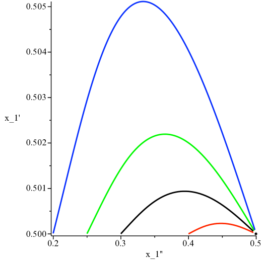
Figure 1: Four one-dimensional slices of the genus-two $\vartheta$-divisor are presented in co-moving coordinates $[x^{\prime}x^{\prime\prime}]$ for the Jacobian. The moduli $\Omega_{11}$, $\Omega_{22}$, and the characteristic $x_{2}^{\prime\prime}$ are chosen “generically”: we set $\Omega_{11}=0.4+i$, $\Omega_{22}=0.1+2i$, and $x_{2}^{\prime\prime}=0.55$. The remaining modulus is chosen to be real $\Omega_{12}=t$ and in the interval $[0,1]$. At $t=0$, we choose $x_{1}^{\prime}=x_{1}^{\prime\prime}=1/2$, a point which is on the $\vartheta$-divisor for any value of $x_{2}^{\prime}$ in view of (B.1). We plot the parametric curves $x_{1}^{\prime}(t)$ versus $x_{1}^{\prime\prime}(t)$ as $t$ runs from 0 to 1, for four values of $x_{2}^{\prime}$, namely $x_{2}^{\prime}=0.1$ (red), $x_{2}^{\prime}=0.2$ (black), $x_{2}^{\prime}=0.25$ (green), and $x_{2}^{\prime}=0.3$ (blue), such that $\vartheta[x](0,\Omega)=0$.

$\bullet$ Genus one

However, the same arguments transposed to genus one lead to a different conclusion, as should have been expected from the explicit formula we have available for the genus-one Faltings invariant. The genus-one equivalent is given by,

$$\partial_{\tau}\partial_{\bar{\tau}}\ln\Phi(\tau)=\int_{T^{2}}d^{2}x\,\Big{|}\dot{x}^{\prime}\,\partial^{\prime}\vartheta[x](0,\tau)+\dot{x}^{\prime\prime}\,\partial^{\prime\prime}\vartheta[x](0,\tau)\Big{|}^{2}\leavevmode\nobreak\ \delta^{(2)}(\vartheta[x](0,\tau)$$ (5.24)

For genus one, the $\vartheta$-divisor is a single point, $\zeta=1/2+\tau/2$, or in terms of characteristics $x^{\prime}=x^{\prime\prime}=1/2$. Thus, $\Theta$ has no intrinsic variation as $\tau$ is being varied, and hence we have,

$$\partial_{\tau}\partial_{\bar{\tau}}\ln\Phi(\tau)=0$$ (5.25)

This result is consistent with the explicit result $\Phi(\tau)=|\eta(\tau)|^{2}$.

6 Issues involved in integrating $\varphi$ over moduli space

The coefficients of the terms in the low energy expansion of the string amplitude at genus two are the integrated invariants,

$$\int_{{\cal M}_{2}}d\mu_{2}\,{\cal B}_{2}^{(p,q)}$$ (6.1)

where $d\mu_{2}=|d^{3}\Omega|^{2}/({\rm det\,}{\rm Im\,}\Omega)^{3}$ is the $Sp(4,{\mathbb{Z}})$-invariant measure on the Siegel upper half space $H_{2}$. This suggests that it is of interest to consider the integral of $\varphi(\Omega)$ over the genus-$2$ moduli space. Although we will not succeed in performing this integral explicitly we will prove that the integral is a well-defined, convergent expression.

To this end we recast $\varphi$ in another alternative form,

$$\varphi(\Omega)=\varphi_{0}+{1\over 2}\sum_{\delta\leavevmode\nobreak\ {\rm even}}\int_{T^{4}}d^{4}x\,\ln\left|{\vartheta[x](0,\Omega)\over\vartheta[\delta](0,\Omega)}\right|^{2}$$ (6.2)

To compute the integration over ${\cal M}_{2}$, one would need to compute the following integral,

$$\Lambda[x]=\int_{{\cal M}_{2}}d\mu_{2}\,\ln\left|{\vartheta[x](0,\Omega)\over\vartheta[0](0,\Omega)}\right|^{2}$$ (6.3)

$\Lambda[x]$ is periodic in each $x$ with period 1, and diverges when $x$ is an odd spin structure. In terms of $\Lambda[x]$, the integral of $\varphi$ over moduli is given by,

$$\int_{{\cal M}_{2}}d\mu_{2}\,\varphi=\varphi_{0}\,V_{2}+5\int_{T^{4}}d^{4}x\Lambda[x]-{1\over 2}\sum_{\delta\leavevmode\nobreak\ {\rm even}}\Lambda[\delta]$$ (6.4)

In order to prove that this integral is convergent we will analyse of the asymptotic properties of the integrand at the boundaries of moduli space where the genus-two surface degenerates, which will be discussed next.

6.1 Asymptotics of the $\varphi$ and $\delta$ invariants in degeneration limits

In this subsection, we shall evaluate the limits of the invariants as the surface approaches the separating and non-separating degeneration nodes. These limits reproduce the genus-two results of [25], where the degeneration limits of the Arakelov Green function and the Faltings invariant on a genus $h$ surface were considered, and the results of [15] on the asymptotic limits of $\varphi$. Here we will start with the expressions for $\delta$ and $\varphi$ in (5.5) and (5.7), rewritten in terms of the modular form $\Phi$ which was defined in (5.9),

$$\delta = 12\ln 2-16\ln(2\pi)-6\ln({\rm det\,}Y)-\ln\left|\Psi_{10}\right|-2\ln\Phi\,,$$ (6.5)

$$\varphi = 6\ln 2-{1\over 2}\ln\left|\Psi_{10}\right|+5\ln\Phi\,.$$ (6.6)

To describe the degenerations we use the following parametrization of the period matrix,

$$\Omega=\left(\matrix{\tau_{1}&\tau\cr\tau&\tau_{2}\cr}\right)\,.$$ (6.7)

The separating degeneration is obtained by sending $\tau\to 0$ while keeping $\tau_{1},\tau_{2}$ fixed. The non-separating degeneration is obtained by letting $\tau_{2}\to i\infty$ while keeping $\tau_{1},\tau$ fixed. Since the behavior of $\Psi_{10}$ at the degenerations is standard, we need only study the asymptotic behavior of $\Phi$ in the appropriate limits, details of which are given in appendix B.

$\bullet$ Separating degeneration node $\tau\to 0$

Substituting the expression for $\Psi_{10}$ near the separating degeneration,

$$\Psi_{10}(\Omega)=-2^{12}(2\pi\tau)^{2}\eta(\tau_{1})^{24}\eta(\tau_{2})^{24}+{\cal O}(\tau^{4})\,,$$ (6.8)

together with the expression for $\Phi$ of (B.8), into (6.6) gives the following limit for the Zhang–Kawazumi invariant $\varphi$,

$$\varphi(\Omega)=-\ln\Big{|}2\pi\tau\eta(\tau_{1})^{2}\eta(\tau_{2})^{2}\Big{|}+{\cal O}(\tau^{2})$$ (6.9)

The Faltings invariant $\delta$ may now be derived from (5.1), and we find,

$$\delta(\Omega)=\delta_{1}(\tau_{1})+\delta_{2}(\tau_{2})-\ln\Big{|}2\pi\tau\eta(\tau_{1})^{2}\eta(\tau_{2})^{2}\Big{|}^{2}+{\cal O}(\tau^{2})$$ (6.10)

where the genus-one Faltings invariant on the degeneration component $I$ has been denoted by $\delta_{I}$, and is given by (see for example [24] after Proposition 4.6),

$$\delta_{I}(\tau_{I})=-8\ln(2\pi)-6\ln\Big{(}({\rm Im\,}\tau_{I})|\eta(\tau_{I})|^{4}\Big{)}\,,$$ (6.11)

a combination which is manifestly modular invariant. The combination $2\pi\tau\eta(\tau_{1})^{2}\eta(\tau_{2})^{2}$, which is invariant under the $Sp(4,{\mathbb{Z}})$ transformations (5.12) to leading order in $\tau$, was identified in [25] as the intrinsic degeneration parameter (and referred to as $\tau$ in that paper). With this identification, our final result (6.10) for the separating degeneration precisely agrees with part $(a)$ of the Main Theorem of [25], specialized to genus $h=2$ and $h_{1}=h_{2}=1$.

$\bullet$ Non-separating degeneration node $\tau_{2}\to i\infty$

Using the non-separating degeneration limit of $\Psi_{10}$,

$$\Psi_{10}(\Omega)=-2^{12}e^{2\pi i\tau_{2}}\eta(\tau_{1})^{18}\vartheta_{1}(\tau,\tau_{1})^{2}$$ (6.12)

and the asymptotics for $\Phi$ of (B.14), we find,

$$\varphi(\Omega) = {\pi\over 6}({\rm Im\,}\tau_{2})+{5\pi\over 6}{({\rm Im\,}\tau)^{2}\over{\rm Im\,}\tau_{1}}-\ln\left|{\vartheta_{1}(\tau,\tau_{1})\over\eta(\tau_{1})}\right|$$ (6.13)

$$\delta(\Omega) = \delta_{1}(\tau_{1})-8\ln(2\pi)+{7\pi\over 3}{\rm Im\,}\tau_{2}-6\ln({\rm Im\,}\tau_{2})-{\pi\over 3}{({\rm Im\,}\tau)^{2}\over{\rm Im\,}\tau_{1}}-2\ln\left|{\vartheta_{1}(\tau,\tau_{1})\over\eta(\tau_{1})}\right|$$

Throughout this subsection we shall neglect contributions which vanish as $\tau_{2}\to i\infty$. Expressed in terms of the Arakelov Green function $\ln g(z)=\ln g(z|\tau_{1})$ for modulus $\tau_{1}$ presented in (B.17), these invariants become,

$$\varphi(\Omega) = {\pi\over 6}\left({\rm Im\,}\tau_{2}-{({\rm Im\,}\tau)^{2}\over{\rm Im\,}\tau_{1}}\right)-\ln g(\tau|\tau_{1})$$ (6.14)

$$\delta(\Omega) = \delta_{1}(\tau_{1})-8\ln(2\pi)+{7\pi\over 3}\left({\rm Im\,}\tau_{2}-{({\rm Im\,}\tau)^{2}\over{\rm Im\,}\tau_{1}}\right)-6\ln({\rm Im\,}\tau_{2})-2\ln g(\tau|\tau_{1})$$

In terms of the modular invariant degeneration parameter $|t|$ which was introduced in [25], and is defined by,

$${\rm Im\,}\tau_{2}-{({\rm Im\,}\tau)^{2}\over{\rm Im\,}\tau_{1}}=-{1\over 2\pi}\ln|t|+{1\over\pi}\ln g(\tau|\tau_{1})$$ (6.15)

the invariants take the following form,

$$\varphi(\Omega) = -{1\over 12}\ln|t|-{5\over 6}\ln g(\tau|\tau_{1})$$ (6.16)

$$\delta(\Omega) = \delta_{1}(\tau_{1})-{7\over 6}\ln|t|-6\ln(-\ln|t|)+{1\over 3}\ln g(\tau|\tau_{1})-2\ln(2\pi)$$

This expression agrees precisely with part $(b)$ of the Main Theorem of [25] for genus two.

6.2 Convergence of the integral over moduli space

The preceding analysis of asymptotic behavior enables us to prove the convergence of the integral of $\varphi$ over the genus-two moduli space ${\cal M}_{2}$ with the measure $d\mu_{2}$, encountered in (6.4). The function $\varphi(\Omega)$ is well-defined everywhere in the interior of ${\cal M}_{2}$, but has singularities as one approaches the boundary of ${\cal M}_{2}$. To deal with the boundary behavior in a systematic way, it will be convenient to replace ${\cal M}_{2}$ by its Deligne-Mumford [26] compactification $\overline{{\cal M}_{2}}$, which is obtained from ${\cal M}_{2}$ by adjoining the divisors (a divisor is a subvariety of complex co-dimension 1) corresponding to the separating node and to the non-separating node. The integration measure $d\mu_{2}$ extends to a finite measure on $\overline{{\cal M}_{2}}$ with finite volume.

To show convergence of the integral of $\varphi$ on the compact space $\overline{{\cal M}_{2}}$, it will suffice to show that the integral converges near each one of the compactification divisors. The divisors intersect, but the convergence of the integral near the intersection will be shown to follow from the convergence near each divisor separately.

$\bullet$ The asymptotic behavior of the measure near the separating divisor $\tau\to 0$ is given by,

$$d\mu_{2}\to|d^{2}\tau|\,\frac{|d^{2}\tau_{1}|}{({\rm Im\,}\tau_{1})^{3}}\,\frac{|d^{2}\tau_{2}|}{({\rm Im\,}\tau_{2})^{3}}\left(1+{\cal O}(|\tau|^{2})\right)\,.$$ (6.17)

Since the most singular term as $\tau\to 0$ is given from (6.9) by $\varphi\sim-\ln|\tau|+\ldots$ the $\tau$ integral converges near $\tau\to 0$, in view of the integration range of (2.1).

$\bullet$ The asymptotic behavior of the measure near the non-separating divisor $\tau_{2}\to i\infty$ is similarly given by the following formula,

$$d\mu_{2}\to|d^{2}\tau|\,\frac{|d^{2}\tau_{1}|}{({\rm Im\,}\tau_{1})^{3}}\,\frac{|d^{2}\tau_{2}|}{({\rm Im\,}\tau_{2})^{3}}\left(1+{\cal O}({\rm Im\,}\tau_{2}^{-1})\right)\,.$$ (6.18)

From (6.13) we see that $\varphi\sim\pi\,{\rm Im\,}\tau_{2}/6+{\cal O}(\tau_{2}^{0})$ so that the $\tau_{2}$ integral converges, in view of the integration range of (2.1).

$\bullet$ The asymptotic behavior near the intersection of the separating and non-separating divisors is given by either formula (6.17) or (6.18) for the measure. The asymptotic behavior of $\varphi$ near the intersection of the divisors may be obtained either as the $\tau_{2}\to i\infty$ asymptotics of (6.9), or as the $\tau\to 0$ asymptotics of (6.14). Happily, these two limits are interchangeable, and give rise to the following uniform asymptotics near the intersection of divisors,

$$\varphi(\Omega)=-\ln(2\pi)+{\pi\over 6}{\rm Im\,}\tau_{2}-\ln|\tau|-\ln|\eta(\tau_{1})|^{2}$$ (6.19)

up to terms that vanish as $\tau\to 0$ and $\tau_{2}\to i\infty$. It is readily seen that the convergence near the intersection is automatic once the convergence near each divisor has been checked.

We conclude that the integral with the measure $d\mu_{2}$ of $\varphi$ over the compactified moduli space $\overline{{\cal M}_{2}}$, and thus over the moduli space ${\cal M}_{2}$, is convergent.

7 Value of integrated invariant from $SL(2,{\mathbb{Z}})$-duality

Although we have not evaluated the integrated invariant directly, we will now determine the relationship of its value to the coefficient of the genus-two $D^{6}\,{\cal R}^{4}$ term in the low energy expansion of the four-string amplitude in Type IIB string theory..

As we described in the introduction, the Type IIB theory is invariant under the duality group $SL(2,{\mathbb{Z}})$, which acts on the complex coupling $T=T_{1}+iT_{2}$ by Möbius transformations. The $SL(2,{\mathbb{Z}})$ transformation properties of the other fields will not concern us here.

Symmetry of the amplitude under the interchange of external states again implies that the low energy expansion of the analytic part of the amplitude is a symmetric function of powers of the Mandelstam variables and has an expansion in powers of $\sigma_{2}$ and $\sigma_{3}$ in which each term is invariant under $SL(2,{\mathbb{Z}})$. These conditions imply that the analytic part of the full (i.e., non-perturbative) amplitude has a low energy expansion of the form,

$${\cal A}^{(4)}(\epsilon_{i},k_{i},T)\Big{|}_{{\rm an.}} = \kappa_{10}^{2}\,{\cal R}^{4}\Big{(}T_{2}^{2}\frac{3}{\sigma_{3}}+T_{2}^{\frac{1}{2}}\,{\cal E}_{(0,0)}(T)\,+T_{2}^{-\frac{1}{2}}\,{\cal E}_{(1,0)}(T)\,\sigma_{2}$$ (7.1)

$$\hskip 72.26999pt+T_{2}^{-1}\,{\cal E}_{(0,1)}(T)\,\sigma_{3}+\ldots\Big{)}\,,$$

where the explicit powers of $T_{2}$ disappear after transforming from the string frame to the Einstein frame (in which the curvature, ${\cal R}$ is inert under $SL(2,{\mathbb{Z}})$). The coefficients ${\cal E}_{(p,q)}(T)$ are $SL(2,{\mathbb{Z}})$-invariant functions. The prefactor of ${\cal R}^{4}$, which arose in the perturbative examples discussed earlier, in fact multiplies the full amplitude as can be deduced from maximal supersymmetry. The first term in the above expansion is the lowest order term in the tree-level expansion, which is equal to the tree-level supergravity amplitude. The challenge is to determine the modular invariant coefficient functions of the higher order terms. These are functions of $T$ and their expansions in the weak-coupling limit $T_{2}\to\infty$ should start with power-behaved terms that correspond to terms in string perturbation theory.

The first term in the $\alpha^{\prime}$ expansion (7.1) beyond the supergravity amplitude is of order ${\cal R}^{4}$, and corresponds to an interaction which preserves 16 supersymmetries in an effective action, that may be expressed as an integral over 16 Grassmann coordinates. The next term is of order $D^{4}{\cal R}^{4}$, which is associated with an effective interaction which preserves 8 supersymmetries, that may be expressed as an integral over 24 superspace Grassmann coordinates. These have $T$-dependent coefficients [5, 6, 7]

$${\cal E}_{(0,0)}(T)=2\zeta(3)\,E_{\frac{3}{2}}(T)\,,\qquad{\cal E}_{(1,0)}(T)=\zeta(5)\,\,E_{\frac{5}{2}}(T)\,,$$ (7.2)

where $E_{s}(T)$ is an $SL(2,{\mathbb{Z}})$ non-holomorphic Eisenstein series, which was encountered earlier in a different context and was defined in (2.30). Although these solutions were initially discovered by indirect means they were subsequently determined by supersymmetry, which constrains the coefficients to satisfy Laplace eigenvalue equations of the form (2.32) with $s=3/2$ (in the ${\cal R}^{4}$) case or $5/2$ (in the $D^{4}{\cal R}^{4}$ case) [6, 7].

The perturbative and non-perturbative content of these coefficients can easily be extracted by considering the Fourier modes of $E_{s}(T)$, defined by

$$2\zeta(2s)\,E_{s}(T)=\sum_{N\neq 0}{\cal F}_{N}(T_{2})\,e^{2i\pi NT_{1}}\,.$$ (7.3)

The non-zero modes ${\cal F}_{N\neq 0}(T_{2})$ contain the effects of D-instantons, with exponentially suppressed asymptotic behavior, ${\cal F}_{N}(T_{2})\sim e^{-2\pi|N|T_{2}}$, at weak coupling ($T_{2}\to\infty$). The zero mode, on the other hand, is a sum of two power behaved terms $T_{2}^{s}$ and $T_{2}^{1-s}$ which correspond to particular terms in string perturbation theory,

$${\cal F}_{0}(T_{2})=2\zeta(2s)\,T_{2}^{s}+\frac{2\pi^{1/2}\Gamma(s-1/2)}{\Gamma(s)}\,\zeta(2s-1)\,T_{2}^{1-s}\,,$$ (7.4)

Substituting the zero mode parts of the coefficients ${\cal E}_{(0,0)}(T)$ and ${\cal E}_{(1,0)}(T)$, as defined in (7.2), into (7.1) gives the contributions that are power-behaved in the coupling constant, Thus, the perturbative contribution to the ${\cal R}^{4}$ term is obtained by setting $s=3/2$,

$$T_{2}^{{1\over 2}}\,\int_{-{1\over 2}}^{1\over 2}{\cal E}_{(0,0)}(T)\,dT_{1}=2\zeta(3)\,T_{2}^{{1\over 2}}\,\int_{-{1\over 2}}^{1\over 2}E_{\frac{3}{2}}(T)\,dT_{1}=2\zeta(3)T_{2}^{2}+4\zeta(2)\,,$$ (7.5)

which contains the sum of tree-level and one-loop contributions. Similarly, the perturbative contribution to the coefficient of $\sigma_{2}\,{\cal R}^{4}$ is

$$T_{2}^{-{1\over 2}}\,\int_{-{1\over 2}}^{1\over 2}{\cal E}_{(1,0)}(T)\,dT_{1}=\zeta(5)\,T_{2}^{-{1\over 2}}\,\int_{-{1\over 2}}^{1\over 2}E_{\frac{5}{2}}(T)\,dT_{1}=\zeta(5)T_{2}^{2}+{4\over 3}\zeta(4)T_{2}^{-2}\,,$$ (7.6)

which contains the sum of tree-level and two-loop contributions. The precise coefficients of the perturbative terms in (7.5) and (7.6) match those determined directly from perturbative string calculations reviewed in section 2.3. The tree-level terms were shown in (2.23) while the genus-one term in (7.5) is given (up to a normalization factor) by $\int d\mu_{1}\,{\cal B}_{1}^{(0,0)}$. Similarly, the genus-two term in (7.6) is given (up to a normalization factor) by $\int d\mu_{2}\,{\cal B}_{2}^{(1,0)}$ [14]. This also accounts for the absence of a one-loop contribution to $\sigma_{2}{\cal R}^{4}$ in the ten-dimensional theory. Generalizations of these results to lower dimensional theories with maximal supersymmetry obtained by toroidal compactification involve combinations of Eisenstein series for higher-rank duality groups, which are functions of more moduli [27, 28, 29] (see also [30]).

The coefficient of the term $D^{6}{\cal R}^{4}$ in the low energy expansion which preserves 4 supersymmetries, ${\cal E}_{0,1}$, is not an Eisenstein series but is expected to be a solution of the inhomogeneous Laplace equation

$$(\Delta_{T}-12)\,{\cal E}_{(0,1)}(T)=-(2\zeta(3)\,E_{\frac{3}{2}})^{2}\,$$ (7.7)

This equation was motivated by M-theory considerations in [8] based on considering the compactification of Feynman diagrams of eleven-dimensional supergravity on a torus. The solution to this equation has an asymptotic expansion for large $T_{2}$ that gives a contribution to the coefficient of the $\sigma_{3}\,{\cal R}^{4}$ term in (7.1) of the form

$$\frac{1}{T_{2}}\int_{-{1\over 2}}^{1\over 2}{\cal E}_{(0,1)}(T)\,dT_{1}=\frac{2}{3}\zeta(3)^{2}T_{2}^{2}+\frac{4}{3}\zeta(2)\zeta(3)+{8\over 5}\zeta(2)^{2}T_{2}^{-2}+{4\over 27}\zeta(6)T_{2}^{-4}+{\cal O}(e^{-2\pi T_{2}})\,$$ (7.8)

which contains four perturbative terms that are power-behaved in $T_{2}$ that correspond to tree-level, one-loop, two-loop and three-loop string theory contributions, together with an infinite sum of D-instanton contributions. The ratio of the tree-level and one-loop contributions agrees with the explicit string perturbation theory calculations and the overall normalization has been chosen to be consistent with a tree-level amplitude normalized to $3/\sigma_{3}$.

We can now compare the ratio of the two-loop perturbative contribution to ${\cal E}_{(0,1)}\,\sigma_{3}\,{\cal R}^{4}$ with the two-loop contribution to ${\cal E}_{(1,0)}\,\sigma_{2}\,{\cal R}^{4}$. First note that the expressions for ${\cal E}_{(1,0)}$ and ${\cal E}_{(0,1)}$ in (7.6) and (7.8) have been normalized to ensure that their tree-level contributions have the correct relative normalizations, which accords with the tree-level expansion of the amplitude as given in (2.23),

$${\cal A}^{(0)}_{4}\Big{|}_{\sigma_{2}\,{\cal R}^{4}+\sigma_{3}\,{\cal R}^{4}}=\kappa_{10}^{2}T_{2}^{2}\left(\zeta(5)\,\sigma_{2}+{2\over 3}\zeta(3)^{2}\,\sigma_{3}\right){\cal R}^{4}.$$ (7.9)

The ratio of two-loop contributions to the $\sigma_{2}\,{\cal R}^{4}$ and $\sigma_{3}\,{\cal R}^{4}$ terms (the $T_{2}^{-2}$ terms in (7.6) and (7.8)) is given by

$$\frac{\int_{{\cal M}_{2}}d\mu_{2}\,{\cal B}_{2}^{(0,1)}}{\int_{{\cal M}_{2}}d\mu_{2}\,{\cal B}_{2}^{(1,0)}}={\frac{8}{5}\zeta(2)^{2}\over\frac{4}{3}\zeta(4)}=3\,.$$ (7.10)

From (3.20) with $h=2$ we see that this means that the integral of the Zhang–Kawazumi invariant should take the value

$$\int_{{\cal M}_{2}}d\mu_{2}\,\varphi=\frac{1}{64}\int_{{\cal M}_{2}}d\mu_{2}\,{\cal B}_{2}^{(0,1)}=\frac{3}{64}\,\int_{{\cal M}_{2}}d\mu_{2}\,{\cal B}_{2}^{(1,0)}=\frac{3}{2}V_{2}=\frac{2\pi^{3}}{45}\,,$$ (7.11)

where $V_{2}=4\pi^{3}/135$ is the volume of ${\cal M}_{2}$ and we have substituted the value ${\cal B}_{2}^{(1,0)}=32$ obtained in (2.39). We note here that, by the construction of $\varphi$ given in (3.14), we have $\varphi(\Omega)>0$ for all $\Omega$, which is consistent with the sign of the proposed relation (7.11).

It would be satisfying to find a method of evaluating $\int_{{\cal M}_{2}}d\mu_{2}\,\varphi$ directly, which would provide a precise check on the $SL(2,{\mathbb{Z}})$-duality prediction and might point to some interesting mathematical properties of $\varphi$.

Acknowledgements:

We thank Richard Wentworth for useful discussions. We also thank Boris Pioline for pointing out an important discrepancy of normalization, by a factor of 2, in the first version of this paper. We are grateful for the support of the National Science Foundation under Grant No. PHYS-1066293 and the hospitality of the Aspen Center for Physics during the Summer of 2011 when this work was started and the Summer of 2013 when it was completed. The research of ED is supported in part by NSF grant PHY-07-57702. MBG also acknowledges funding from the European Research Council under the European Community’s Seventh Framework Programme (FP7/2007-2013) / ERC grant agreement no. [247252].

Appendix A Expressing $\varphi$ as a single integral over $\Sigma$

For completeness, we here determine a second alternative expression for $\varphi$ based on [12, 13] that is given in terms of a single integral over the surface $\Sigma$. To obtain this expression, we start from the following expression for the Faltings invariant, given in [12],

$$\delta(\Omega)=-12\ln(2\pi)-2\ln{\rm det\,}Y-2\ln|{\cal M}_{\nu_{p}\nu_{q}}|+\int_{\Theta+p-q}\mu\ln\|\vartheta\|^{2}$$ (A.1)

In this formula, $p,q$ are two distinct branch points, and $\nu_{p}$ and $\nu_{q}$ their associated odd spin structures. The expression for $\delta(\Omega)$ is independent of the choice made for $p,q$. The modular object ${\cal M}_{\nu_{p}\nu_{q}}$ entered the calculations of the genus-two superstring measure in [31], and may be expressed with the help of $\vartheta$-constants and of the six distinct genus-two odd spin structures $\nu_{i}$ with $i=1,\cdots,6$,

$${\cal M}_{\nu_{i}\nu_{j}}^{2}=\pi^{4}\prod_{k\not=i,j}\vartheta[\nu_{i}+\nu_{j}+\nu_{k}](0,\Omega)^{4}$$ (A.2)

Finally, $\Theta$ is the $\vartheta$-divisor, namely the set of points $\zeta\in J(\Omega)$ such that $\vartheta(\zeta,\Omega)=0$. Using the Riemann vanishing theorem in genus-two, $\Theta$ may be parametrized as follows,

$$\Theta=\left\{\zeta_{I}=\int^{z}_{z_{0}}\omega_{I}-\Delta_{I}(z_{0}),\leavevmode\nobreak\ \leavevmode\nobreak\ z\in\Sigma\right\}$$ (A.3)

where $\Delta_{I}(z_{0})$ is the Riemann vector defined in(3.11). Next, we proceed to reformulate the integral over the shifted $\vartheta$-divisor in terms of more familiar objects. To do so, we use the relation $\nu_{p}=p-\Delta$ to recast the $\vartheta$-function into one with spin structure characteristic $\nu_{p}$,

$$\ln\|\vartheta(z+p-q-\Delta,\Omega)\|^{2} = \ln|\vartheta[\nu_{p}](z-q,\Omega)|^{2}+{1\over 2}\ln({\rm det\,}Y)$$ (A.4)

$$-2\pi\sum_{I,J}Y^{-1}_{IJ}\left({\rm Im\,}\int^{z}_{q}\omega_{I}\right)\left({\rm Im\,}\int^{z}_{q}\omega_{J}\right)$$

We make use of the prime form expressed with respect to spin structure $\nu_{p}$,

$$E(z,w)={\vartheta[\nu_{p}](z-w,\Omega)\over h_{\nu_{p}}(z)\,h_{\nu_{p}}(w)}$$ (A.5)

for $w=q$, where $h_{\nu}(z)$ is the normalized holomorphic 1/2 form with odd spin structure $\nu$. Recasting the first term in (A.4) in terms of the prime form, we find,

$$\ln\|\vartheta(z+p-q-\Delta,\Omega)\|^{2} = \ln|E(z,q)|^{2}+\ln|h_{\nu_{p}}(z)|^{2}+\ln|h_{\nu_{p}}(q)|^{2}$$ (A.6)

$$+{1\over 2}\ln({\rm det\,}Y)-2\pi{\rm Im\,}(z-q)^{t}Y^{-1}{\rm Im\,}(z-q)$$

Combining the first and the last terms, we recognize the appearance of $-G(z,q)$, where the scalar Green function $G$ was defined in (2.17). Putting all together, $\varphi$ takes the form,

$$\varphi(\Omega) = \tilde{\varphi}_{0}-{1\over 2}\ln|\Psi_{10}|-5\ln\left|{h_{\nu_{p}}(q)^{2}\over{\cal M}_{\nu_{p},\nu_{q}}}\right|+5\int_{\Sigma}\mu_{\Sigma}(z)\left\{G(z,q)-\ln|h_{\nu_{p}}(z)|^{2}\right\}$$ (A.7)

Note that the combination $h_{\nu_{p}}(q)^{2}/{\cal M}_{\nu_{p},\nu_{q}}$ is independent of the branch point $\nu_{p}$. Given that the total expression for $\varphi$ is independent of the branch points $p,q$, we see that the integral in (A.7) must be independent of the branch point $p$.

Appendix B Derivation of asymptotic limits of $\Phi$

In this appendix we derive the asymptotic limits quoted in section 6.1.

B.1 The separating degeneration

To leading order in the separating degeneration $\tau\to 0$, the genus-two $\vartheta$-function tends to,

$$\vartheta\left[\matrix{x_{1}^{\prime}&x_{1}^{\prime\prime}\cr x_{2}^{\prime}&x_{2}^{\prime\prime}\cr}\right](0,\Omega)=\vartheta[x_{1}^{\prime}\leavevmode\nobreak\ x_{1}^{\prime\prime}](0,\tau_{1})\,\vartheta[x_{2}^{\prime}\leavevmode\nobreak\ x_{2}^{\prime\prime}](0,\tau_{2})+{\cal O}(\tau^{2})$$ (B.1)

where $\vartheta[x_{I}^{\prime}\leavevmode\nobreak\ x_{I}^{\prime\prime}](0,\tau_{I})$ are the genus-one $\vartheta$-functions with real characteristics $x_{I}^{\prime}\leavevmode\nobreak\ x_{I}^{\prime\prime}$, defined in (2.18). They may be expressed in terms of the $\vartheta$-function with zero characteristics by,

$$\vartheta[x_{I}^{\prime}\leavevmode\nobreak\ x_{I}^{\prime\prime}](0,\tau_{I})=e^{\pi i\tau_{I}(x_{I}^{\prime})^{2}+2\pi ix_{I}^{\prime}x_{I}^{\prime\prime}}\vartheta(x_{I}^{\prime}\tau_{I}+x_{I}^{\prime\prime},\tau_{I})$$ (B.2)

The limit of $\Phi$ then becomes,

$$\ln\Phi=\prod_{I=1}^{2}\left(\int_{0}^{1}dx_{I}^{\prime}\int_{0}^{1}dx_{I}^{\prime\prime}\,\ln|\vartheta[x_{I}^{\prime}\leavevmode\nobreak\ x_{I}^{\prime\prime}](0,\tau_{I})|^{2}\right)+{\cal O}(\tau^{2})$$ (B.3)

To evaluate each factored integral, we first express the $\vartheta$-function with characteristics in terms of $\vartheta$ with zero characteristics using (B.2), and then use the infinite product representation of the latter,

$$\ln\vartheta(z,\tau)=\sum_{n=1}^{\infty}\ln\left[\left(1-e^{2\pi in\tau}\right)\left(1-e^{\pi i(2n\tau+2z-1-\tau)}\right)\left(1-e^{\pi i(2n\tau-2z-1-\tau)}\right)\right]\,.$$ (B.4)

The $x^{\prime}$ and $x^{\prime\prime}$ integrals in (B.3) may be carried out by considering each of the three factors in the square parentheses in turn, as follows. The first factor trivially gives

$$\int_{0}^{1}\!dx^{\prime}_{I}\int_{0}^{1}\!dx^{\prime\prime}_{I}\,\sum_{n=1}^{\infty}\ln\left(1-e^{2\pi in\tau}\right)=\sum_{n=1}^{\infty}\ln\left(1-e^{2\pi in\tau}\right)\,.$$ (B.5)

The second factor contributes zero, since the logarithm has a Taylor expansion in powers of the exponential in its argument and the modulus of the exponential is strictly less than $1$. Each term in the Taylor series vanishes by virtue of the $x^{\prime\prime}$ integral. In the third factor, terms with $n>1$ vanish analogously, but for the $n=1$ term the expansion breaks down when ${1\over 2}\leq x^{\prime}\leq 1$. Thus, that region needs to be re-expanded by writing the argument of the logarithm as $(1-e^{\pi i(\tau-x^{\prime}\tau-2x^{\prime\prime}-1)})=-e^{\pi i(\tau-2x^{\prime}\tau-2x^{\prime\prime}-1)}(1-e^{-\pi i(\tau-2x^{\prime}\tau-2x^{\prime\prime}-1)})$ leading to a non-zero contribution given by

$$\int_{1\over 2}^{1}\!dx^{\prime}_{I}\int_{0}^{1}\!dx^{\prime\prime}_{I}\,i\pi\left((1-2x^{\prime})\tau-2x^{\prime\prime}-1\right)+i\pi=-\frac{1}{4}i\pi\tau\,.$$ (B.6)

In addition to the above terms, in converting from $\ln\vartheta(z,\tau)$ to $\log\vartheta[x^{\prime},x^{\prime\prime}](0,\tau)$ using (B.2) we also need to evaluate the logarithm of the prefactor

$$\pi i\int_{0}^{1}\!dx^{\prime}\int_{0}^{1}\!dx^{\prime\prime}\,(\tau(x^{\prime})^{2}+2x^{\prime}x^{\prime\prime})=\pi i\int_{0}^{1}\!dx^{\prime}\,(\tau(x^{\prime})^{2}+x^{\prime})=\frac{1}{3}i\pi\tau+{1\over 2}i\pi$$ (B.7)

Combining (B.5), (B.6), and (B.7), the final result is

$$\int_{0}^{1}\!dx^{\prime}_{I}\int_{0}^{1}\!dx^{\prime\prime}_{I}\,\ln|\vartheta[x_{I}^{\prime}\leavevmode\nobreak\ x_{I}^{\prime\prime}](0,\tau_{I})|^{2}=\ln\left|\eta(\tau_{I})\right|^{2}$$

As a result, the asymptotics of $\Phi$ is given by

$$\Phi=|\eta(\tau_{1})\eta(\tau_{2})|^{2}+{\cal O}(\tau^{2})\,.$$ (B.8)

B.2 Non-separating degeneration

In terms of the parametrization (6.7) the non-separating degeneration is given by $\tau_{2}\to i\infty$. Later on, we shall be more precise in the finite part of this limit. To extract the leading asymptotics of the genus-two $\vartheta$-function, given by (5.3), we isolate the $\tau_{2}$-dependence by recasting the double sum over $n_{1},n_{2}$ as a simple sum over $n=n_{2}$ of genus-one $\vartheta$-functions. For brevity, we shall use the notation $x_{I}=x_{I}^{\prime}$ and $y_{I}=x_{I}^{\prime\prime}$. We find,

$$\vartheta[x](0,\Omega) = \sum_{n\in{\mathbb{Z}}}C_{n}\,\vartheta(x_{1}\tau_{1}+(n+x_{2})\tau+y_{1},\tau_{1})$$ (B.9)

$$C_{n} = \exp i\pi\Big{\{}\tau_{1}x_{1}^{2}+\tau_{2}(n+x_{2})^{2}+2\tau x_{1}(n+x_{2})+2x_{1}y_{1}+2(n+x_{2})y_{2}\Big{\}}$$

The leading asymptotics depends on the range chosen for the value of the characteristics. To obtain the asymptotics in as simple a manner as possible, we choose the integration ranges for the torus to be $-{1\over 2}\leq x_{I}^{\prime},x_{I}^{\prime\prime}\leq{1\over 2}$. With this choice, it is the term $n=0$ which dominates, and we find the following asymptotics, to leading order,

$$\vartheta[x](0,\Omega)=C_{0}\,\vartheta(\tau_{1}x_{1}+\tau x_{2}+y_{1},\tau_{1})$$ (B.10)

The term in $\tau x_{2}$ may be decomposed by making the following change of variables,

$$x_{1} \to \tilde{x}_{1}=x_{1}+x_{2}({\rm Im\,}\tau)/({\rm Im\,}\tau_{1})$$

$$y_{1} \to \tilde{y}_{1}=y_{1}+x_{2}\Big{(}{\rm Re\,}(\tau)-({\rm Im\,}\tau)({\rm Re\,}\tau_{1})/({\rm Im\,}\tau_{1})\Big{)}$$ (B.11)

in terms of which the leading asymptotics of $\ln|\vartheta|^{2}$ becomes,

$$\ln|\vartheta[x](0,\Omega)|^{2}=\ln|\vartheta[\tilde{x}_{1}\leavevmode\nobreak\ \tilde{y}_{1}](0,\tau_{1})|^{2}-2\pi x_{2}^{2}\,{{\rm det\,}Y\over{\rm Im\,}\tau_{1}}$$ (B.12)

where ${\rm det\,}Y={\rm det\,}{\rm Im\,}\Omega=({\rm Im\,}\tau_{1})({\rm Im\,}\tau_{2})-({\rm Im\,}\tau)^{2}$. Using translation invariance of the integration measure over the torus $T^{4}$, we have $dx_{1}dy_{1}=d\tilde{x}_{1}d\tilde{y}_{1}$ and the integration range is unchanged by periodicity. Carrying out the integrations over $x_{2}$ and $y_{2}$, we find,

$$\ln\Phi=\int_{-{1\over 2}}^{1\over 2}d\tilde{x}_{1}\int_{-{1\over 2}}^{1\over 2}d\tilde{y}_{1}\left(\ln|\vartheta[\tilde{x}_{1}\leavevmode\nobreak\ \tilde{y}_{1}](0,\tau_{1})|^{2}-{\pi\over 6}\,{{\rm det\,}Y\over{\rm Im\,}\tau_{1}}\right)$$ (B.13)

Using the result of (B.1) and (B.8) for the remaining integral, we find,

$$\ln\Phi=\ln|\eta(\tau_{1})|^{2}-{\pi\over 6}\,\left({\rm Im\,}\tau_{2}-{({\rm Im\,}\tau)^{2}\over{\rm Im\,}\tau_{1}}\right)$$ (B.14)

Finally, we shall work out the orders of the terms that we have omitted by retaining only the leading order in $\tau_{2}\to i\infty$. We use the decomposition of the genus-two $\vartheta$-function in (B.9), still for the characteristics $-{1\over 2}\leq x_{I},y_{I}\leq{1\over 2}$. The suppression factors are governed by the ratio of the correction terms, divided by the leading term, and take the form,

$$\left|{C_{n}\over C_{0}}\right|=\exp 2\pi\Big{\{}-({\rm Im\,}\tau_{2})(n^{2}+2nx_{2})-2{\rm Im\,}(\tau)x_{1}n\Big{\}}$$ (B.15)

Since $n^{2}+2nx_{2}\geq|n|(|n|-2|x_{2}|)$, the contributions with $|n|\geq 2$ are suppressed by at least positive integer powers of $e^{-2\pi{\rm Im\,}(\tau_{2})}$. For $n=\pm 1$, the suppression is lesser, and is given by

$$\exp 2\pi\Big{\{}-({\rm Im\,}\tau_{2})(1\pm 2x_{2})\mp 2({\rm Im\,}\tau)x_{1}\Big{\}}{\vartheta(x_{1}\tau_{1}+(x_{2}\pm 1)\tau+y_{1},\tau_{1})\over\vartheta(x_{1}\tau_{1}+x_{2}\tau+y_{1},\tau_{1})}$$ (B.16)

Upon integration over $x_{2}$ in the range $-{1\over 2}\leq x_{2}\leq{1\over 2}$, the correction is found to be power law suppressed by a factor $({\rm Im\,}\tau_{2})^{-1}$. Thus, the terms we have neglected are either exponentially suppressed for $|n|\geq 2$ and power suppressed for $|n|=1$.

B.3 The genus-one Arakelov Green function

The genus-one Green function is standard up to normalization choices. The canonically normalized Green function $G$ was given in (2.25) while the Arakelov normalization is obtained by fixing the arbitrary additive constant in the Green function so that the integral of the Arakelov Green function $\ln g$ vanishes. In the notation of (3.2), we find

$$\ln g(z)=\ln\left|{\vartheta_{1}(z,\tau)\over\eta(\tau)}\right|-{\pi({\rm Im\,}z)^{2}\over{\rm Im\,}\tau}$$ (B.17)

We recall the product formula for $\vartheta_{1}(z,\tau)$,

$$\vartheta_{1}(z,\tau)=-2e^{i\pi\tau/4}\sin(\pi z)\prod_{m=1}^{\infty}\left(1-e^{2\pi im\tau}\right)\left(1-e^{2\pi im\tau+2\pi iz}\right)\left(1-e^{2\pi im\tau-2\pi iz}\right)$$ (B.18)

The Arakelov Green function satisfies,

$$\int_{\Sigma}d^{2}z\ln g(z-w)=0$$ (B.19)

The integral is over the fundamental domain of the genus-one surface $\Sigma$ generated by the lattice with periods $1$ and $\tau_{1}$. Note that the canonical Green function $G$ in (2.25) and the Arakelov Green function $\ln g$ in (B.17) are related by

$$G(z,w)=-2\ln g(z-w)+2\ln(2\pi|\eta|^{2})\,,$$ (B.20)

where we have used the fact that $\vartheta^{\prime}(0,\tau)=-2\pi\eta(\tau)^{3}$.

Appendix C Direct calculation of separating degeneration of $\varphi$

We calculate the separating degeneration asymptotics of $\varphi$ directly from the formula for $\varphi$ given in (3.21), with $G$ defined in (2.17), and $P$ defined in (3.4). In the parametrization of (6.7), we seek the asymptotics as $\tau\to 0$ while keeping $\tau_{I},\leavevmode\nobreak\ I=1,2$ fixed. The surface $\Sigma$ pinches off to the union of two genus 1 surfaces $\Sigma_{I}$ with one puncture $p_{I}$ each.

The leading asymptotics of the normalized holomorphic Abelian differentials $\omega^{t}_{I}$ on the genus-two surface is given by $\omega^{t}_{I}(z)=\omega_{I}^{(1)}(z)+{\cal O}(t)$ for $z\in\Sigma_{I}$ and $\omega^{t}_{I}(z)={\cal O}(t)$ for $z\not\in\Sigma_{I}$, with $\tau=\pi it/2+{\cal O}(t^{2})$. Here, $\omega_{I}^{(1)}$ are the normalized holomorphic Abelian differentials on the genus-one components $\Sigma_{I}$. Representing $\Sigma_{I}$ by a flat torus with modulus $\tau_{I}$, and complex coordinates $z_{I},\bar{z}_{I}$ with periods $1$ and $\tau_{I}$, we have $\omega_{I}^{(1)}(z)=dz_{I}$. The imaginary part of the period matrix becomes, $Y_{IJ}=\delta_{IJ}{\rm Im\,}\tau_{I}+{\cal O}(t)$. Using this information, we evaluate the degeneration limit of the form $P(x,y)$ of (3.4) and we find to leading order,

$$z,w\in\Sigma_{I}\leavevmode\nobreak\ \leavevmode\nobreak\ \leavevmode\nobreak\ P(z,w)=-4({\rm Im\,}\tau_{I})^{-2}d^{2}zd^{2}w$$

$$z\in\Sigma_{1},\leavevmode\nobreak\ w\in\Sigma_{2} P(z,w)=4({\rm Im\,}\tau_{1})^{-1}({\rm Im\,}\tau_{2})^{-1}d^{2}zd^{2}w$$ (C.1)

where we recall that $d^{2}z=idz\wedge d\bar{z}/2$, so that $\int_{\Sigma_{I}}d^{2}z_{I}={\rm Im\,}\tau_{I}$. The asymptotics of the Green function $G$ was carefully evaluated in formula (3.19) of [14], and is given by,

$$z,w\in\Sigma_{I}\leavevmode\nobreak\ \leavevmode\nobreak\ \leavevmode\nobreak\ G(z,w)=G^{(1)}(z,w;\tau_{I})+{\cal O}(\tau)$$ (C.2)

$$z\in\Sigma_{1},\leavevmode\nobreak\ w\in\Sigma_{2} G(z,w)=\ln{|\tau|\over 2\pi}+G^{(1)}(z,p_{1},\tau_{1})+G^{(1)}(w,p_{2};\tau_{2})+{\cal O}(\tau)$$

To make its genus-one nature and modulus explicit, we have denoted the genus-one Green function of (2.19) for modulus $\tau_{I}$ by $G^{(1)}(z,w;\tau_{I})$.

To carry out the integrals of (3.21) in this limit, we proceed from (B.19) and (B.20), to deduce the value of the following integral,

$$\int_{\Sigma_{I}}d^{2}z_{I}G^{(1)}(z_{I},w;\tau_{I})=2({\rm Im\,}\tau_{I})\ln(2\pi|\eta(\tau_{I})|^{2})$$ (C.3)

for any point $w$ (as follows by translation invariance on the torus). Combining the limits of $P$ and $G$ given above, and carrying out the integrals over $z$ and $w$, we find,

$$\varphi = +\ln(2\pi|\eta(\tau_{1})|^{2})+\ln(2\pi|\eta(\tau_{2})|^{2})$$ (C.4)

$$-\ln{|\tau|\over 2\pi}-2\ln(2\pi|\eta(\tau_{1})|^{2})-2\ln(2\pi|\eta(\tau_{2})|^{2})$$

The terms on the first line result from the integration over $z,w$ on the same component $\Sigma_{I}$, while the terms on the second line arise from $z$ and $w$ on opposite components $\Sigma_{I}$. The contribution from points in the funnel (present for non-zero $t$) tends to 0 as $t\to 0$, and may be neglected. Minor simplification reproduces the separating degeneration asymptotics of (6.9), which was obtained through the asymptotics from $\Phi$ in appendix B.

References

- [1] E. D’Hoker and D. H. Phong, “Two loop superstrings. 1. Main formulas,” Phys. Lett. B 529, 241 (2002) [hep-th/0110247].
- [2] E. D’Hoker and D. H. Phong, “Two-loop superstrings VI: Non-renormalization theorems and the 4-point function,” Nucl. Phys. B 715, 3 (2005) [hep-th/0501197].
- [3] E. D’Hoker and D. H. Phong, “Lectures on two loop superstrings,” Conf. Proc. C 0208124, 85 (2002) [hep-th/0211111].
- [4] N. Berkovits and C. R. Mafra, “Equivalence of two-loop superstring amplitudes in the pure spinor and RNS formalisms,” Phys. Rev. Lett. 96, 011602 (2006) [hep-th/0509234].
- [5] M. B. Green and M. Gutperle, “Effects of D instantons,” Nucl. Phys. B 498 (1997) 195 [hep-th/9701093].
- [6] M. B. Green and S. Sethi, “Supersymmetry constraints on type IIB supergravity,” Phys. Rev. D 59 (1999) 046006 [hep-th/9808061].
- [7] A. Sinha, “The term in IIB supergravity,” JHEP 0208 (2002) 017 [hep-th/0207070].
- [8] M.B. Green and P. Vanhove, Duality and higher derivative terms in M theory, JHEP 0601 (2006) 093 [arXiv:hep-th/0510027].
- [9] S.W. Zhang, “Gross - Schoen Cycles and Dualising Sheaves” Inventiones mathematicae, Volume 179, Issue 1, pp 1-73 arXiv:0812.0371
- [10] N. Kawazumi, “Johnson’s homomorphisms and the Arakelov Green function”, arXiv:0801.4218 [math.GT].
- [11] R. De Jong, “Second variation of Zhang’s -invariant on the moduli space of curves”, arXiv:1002.1618v2.
- [12] J.-B. Bost, “Fonctions de Green-Arakelov, fonctions theta et courbes de genre 2”, C. R. Acad. Sci. Paris, t. 305, série I, p. 643-646, 1987
- [13] J.-B. Bost, J.-F. Mestre, L. Morey-Bailly, “Sur le calcul explicite des classes de Chern des surfaces arithmétiques de genre 2”, in Séminaire sur les pinceaux de courbes elliptiques, Astérique 183 (1990) 69-105.
- [14] E. D’Hoker, M. Gutperle and D. H. Phong, “Two-loop superstrings and S-duality,” Nucl. Phys. B 722 (2005) 81 [arXiv:hep-th/0503180].
- [15] R. De Jong, “Asymptotic behavior of the Kawazumi-Zhang invariant for degenerating Riemann surfaces”, arXiv:1207.2353
- [16] M. B. Green, J. H. Schwarz and E. Witten, Superstring Theory. Vol. 1: Introduction, Cambridge, Uk: Univ. Pr. (1987) (Cambridge Monographs On Mathematical Physics)
- [17] H. Klingen, Introductory Lectures to Siegel Modular Forms, Cambridge University Press, 1990
- [18] M. B. Green and P. Vanhove, “The Low-energy expansion of the one loop type II superstring amplitude,” Phys. Rev. D 61 (2000) 104011 [hep-th/9910056].
- [19] M. B. Green, J. G. Russo and P. Vanhove, “Low energy expansion of the four-particle genus-one amplitude in type II superstring theory,” JHEP 0802 (2008) 020 [arXiv:0801.0322 [hep-th]].
- [20] M. B. Green and J. H. Schwarz, “Supersymmetrical String Theories,” Phys. Lett. B 109, 444 (1982).
- [21] E. D’Hoker and D. H. Phong, “The Box graph in superstring theory,” Nucl. Phys. B 440, 24 (1995) [hep-th/9410152].
- [22] O. Schlotterer and S. Stieberger, “Motivic Multiple Zeta Values and Superstring Amplitudes,” arXiv:1205.1516 [hep-th].
- [23] M. B. Green, C. R. Mafra and O. Schlotterer, “Multiparticle one-loop amplitudes and S-duality in closed superstring theory,” arXiv:1307.3534 [hep-th].
- [24] R. De Jong, “Arakelov Invariants of Riemann surfaces”, Documenta Mathematica 10 (2005) 311 329
- [25] R. Wentworth “The Asymptotics of the Arakelov-Green’s Function and Faltings’ Delta Invariant”, Commun. Math. Phys. 137, 427-459 (1991)
- [26] P. Deligne and D. Mumford, Publ. Math. IHES 36 (1979) page 75.
- [27] N. A. Obers and B. Pioline, “Eisenstein series and string thresholds,” Commun. Math. Phys. 209, 275 (2000) [hep-th/9903113].
- [28] M. B. Green, J. G. Russo and P. Vanhove, “Automorphic properties of low energy string amplitudes in various dimensions,” Phys. Rev. D 81 (2010) 086008 [arXiv:1001.2535 [hep-th]].
- [29] M. B. Green, S. D. Miller, J. G. Russo and P. Vanhove, “Eisenstein series for higher-rank groups and string theory amplitudes,” Commun. Num. Theor. Phys. 4 (2010) 551 [arXiv:1004.0163 [hep-th]].
- [30] B. Pioline, “R**4 couplings and automorphic unipotent representations,” JHEP 1003, 116 (2010) [arXiv:1001.3647 [hep-th]].
- [31] E. D’Hoker and D. H. Phong, “Two loop superstrings 4: The Cosmological constant and modular forms,” Nucl. Phys. B 639, 129 (2002) [hep-th/0111040].