Unifying Three Perspectives on Information Processing in Stochastic Thermodynamics
Abstract
So far, feedback-driven systems have been discussed using (i) measurement and control, (ii) a tape interacting with a system or (iii) by identifying an implicit Maxwell demon in steady state transport. We derive the corresponding second laws from one master fluctuation theorem and discuss their relationship. In particular, we show that both the entropy production involving mutual information between system and controller and the one involving a Shannon entropy difference of an information reservoir like a tape carry an extra term different from the usual current times affinity. We thus generalize stochastic thermodynamics to the presence of an information reservoir.
pacs:
05.70.Ln, 05.40.-a, 89.70.CfA deep relation between information theory and statistical physics has been apparent from the very conception of the former in Shannon’s classical formulation Shannon (1948); Jaynes (1957). One explicit manifestation is Bennett’s insight on how Landauer’s result on the thermodynamic cost of erasing memory exorcises Maxwell’s demon Bennett (1982); Maruyama et al. (2009). While thus the universal validity of the second law has apparently been restored, exploring the specific relationship between information theory and thermodynamics particularly in small systems has become a very active field not the least since ingenious experiments with single colloidal particles provide beautiful illustrations and test of these concepts Toyabe et al. (2010); Bérut et al. (2012). If the arguably bewildering plethora of recent theoretical work in this field Touchette and Lloyd (2000, 2004); Cao et al. (2004); Cao and Feito (2009); Sagawa and Ueda (2010); Ponmurugan (2010); Horowitz and Vaikuntanathan (2010); Horowitz and Parrondo (2011a, b); Granger and Kantz (2011); Abreu and Seifert (2011, 2012); Kundu (2012); Sagawa and Ueda (2012a, b); Bauer et al. (2012); Kish and Granqvist (2012); Mandal and Jarzynski (2012); Barato and Seifert (2013); Mandal et al. (2013); Esposito and Schaller (2012); Strasberg et al. (2013); Horowitz et al. (2013); Granger and Kantz (2013); Kawai et al. (2007); Esposito and van den Broeck (2011); Andrieux and Gaspard (2008); andr13 is tentatively classified into three main approaches an important question on the uniqueness of the second law arises as follows.
In the first and most prominent approach, the classical ideas of Maxwell and Szilard are implemented in an explicit feedback scheme where immediately after a measurement some parameters of the device are altered depending on the outcome of the measurement Touchette and Lloyd (2000, 2004); Cao et al. (2004); Cao and Feito (2009); Sagawa and Ueda (2010); Ponmurugan (2010); Horowitz and Vaikuntanathan (2010); Horowitz and Parrondo (2011a, b); Granger and Kantz (2011); Abreu and Seifert (2011, 2012); Kundu (2012); Sagawa and Ueda (2012a, b); Bauer et al. (2012); Kish and Granqvist (2012). The subsequent evolution of the system thus depends on the state after the measurement and the new control parameter. For such a set-up, Sagawa and Ueda have derived an integral fluctuation theorem (FT) Sagawa and Ueda (2010). The corresponding inequality implies that the extracted work, which from the perspective of the first law is compensated by a corresponding heat transfer from the bath, is less than the information acquired in the measurement Cao and Feito (2009). This inequality thus generalizes the second law to such feedback-driven schemes. Since the thermodynamic cost of neither the measurement nor of the erasure of the acquired information are included, the analysis is necessarily somewhat incomplete from a thermodynamic point of view.
A second approach where the system is allowed to interact explicitly with an information storage device such as a tape consisting of a sequence of bits overcomes this deficiency. In such a scheme, an inequality has been derived which shows that the work extracted from a heat bath is necessarily less than the information theoretic entropy difference between outgoing and incoming tape Mandal and Jarzynski (2012) (see also Barato and Seifert (2013); Mandal et al. (2013)). How is this inequality related to the one derived in the first approach? Does it also follow from an underlying fluctuation theorem?
In the third approach, “ordinary” transport through a device like a quantum dot controlled by a gate is considered Esposito and Schaller (2012); Strasberg et al. (2013). The corresponding non-equilibrium steady state (NESS) complies with the well-established rules of stochastic thermodynamics including a well-defined rate of thermodynamic entropy production Seifert (2012). A posteriori, however, a term in the entropy production is interpreted as an “information current”, which is related to an idealized feedback procedure happening much faster than the time-scales for the transitions between states. Again, the question arises whether and how the genuine thermodynamic entropy production of a NESS relates to the second laws discussed within the first two approaches. A recent work in this direction compares this genuine entropy production with the one arising from the first approach by considering two models with similar dynamics that can be either driven by an input of chemical work or by feedback Horowitz et al. (2013).
In this letter, we will show that the second laws arising from these three approaches are in fact three different inequalities involving three different quantities each bounding the maximal extractable work from such devices. We will do so by first discussing the simplest paradigmatic device based on a two level system from all three perspectives. For a system with an arbitrary number of states, we then derive one master FT which can be specialized to yield the three second laws pertaining to the three perspectives discussed above. Based on these insights, we can thus generalize stochastic thermodynamics to include an information reservoir, like a a tape that mediates transitions between a pair of states in a general NESS. Surprisingly, differing from the usual thermodynamic entropy production which can be written as a sum of currents multiplied by affinities, the contribution due to the information reservoir does not involve a current.
Let us set the stage with a paradigmatic two level system Esposito et al. (2010); Kumar et al. (2011); Cao and Feito (2009); Horowitz et al. (2013). The upper level has energy and the lower level has energy . The system is connected to a heat bath at temperature so that the transition rates fulfill the detailed balance relation , where we set Boltzmann’s constant multiplied by the temperature to , is the transition rate from to , and is the reversed one. The feedback is introduced in the following way. After every period a measurement gives information to a controller whether the state of the system is or . If the measurement is error free and if at the end of the time interval the system is at , the energy of the upper level is lowered to , leading to the extraction of work . Furthermore, the energy of the empty state is elevated to at no cost. This instantaneous change in the energy levels of the system corresponds to an effective jump from state to state , because after the energy levels are switched the labels are also switched with always representing the state with energy and the state with energy .
More generally, we assume a probability of a measurement error given by , so that if the state at time is () the measurement yields () with probability and () with probability . Moreover, for the energy levels are interchanged and for they remain fixed. Note that whenever an error occurs the initial state in the next time interval is . Hence, the system reaches a periodic steady state for which the probability of finishing the period at state is
| (1) |
where and . The mean extracted work per time interval is given by
| (2) |
The probability of the measurement outcome is
| (3) |
while the probability for is . Therefore, the Shannon entropy of the controller is . This Shannon entropy conditioned on the state of the system becomes footnote . Using the standard definition for the mutual information between the system and the controller cove06 , we obtain . The second law of thermodynamics for feedback controlled systems, then implies Cao and Feito (2009)
| (4) |
i.e., the extracted work is bounded by the mutual information due to measurements.
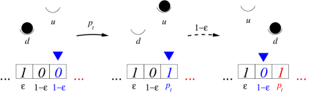
This very model allows a second interpretation which leads to another second law like inequality, see Fig. 1. We now consider a system connected to a thermal bath, mediating the interaction between a work reservoir and a tape (a sequence of bits), which corresponds to a simplified version of the original model proposed in Mandal and Jarzynski (2012). In this interpretation each bit from the tape interacts for a time with the system. During this time interval the bit state () is coupled to the system state (), so that when the system jumps from () to () the bit changes from () to (). After interacting with the system for a time , the bit moves forward, and a new bit comes to interact with the tape. This new incoming bit generates effective transitions by determining the initial state of the system for the subsequent interaction time interval, where for an incoming the system will start at and for an incoming at . More precisely, if the system finishes in state () and the new incoming bit is () then the energy levels are interchanged, leading to an amount of energy extracted from (delivered to) the system. If the system finishes in state () and the new incoming bit is () then the energy levels remain fixed and no energy is exchanged with the work reservoir. Furthermore, the probability of an incoming is and hence the Shannon entropy of the incoming tape is . On the other hand, the outgoing tape is a record of the interaction with the system, with the probability of a being and the Shannon entropy . Importantly, in this second interpretation, we have an autonomous system with no explicit measurement and feedback, the new incoming bit simply determines the initial state of the system for the coming interaction period.
Mandal and Jarzynski Mandal and Jarzynski (2012) showed that a second law like inequality bounds the work (2) delivered to the reservoir by the Shannon entropy difference between the incoming and the outgoing tapes, i.e.,
| (5) |
where is the Kullback-Leibler distance. Hence, as our first result, we realize that this two level system allows for two different interpretations leading to two different second law like inequalities. Since footnote , the bound on the extracted work (5) is tighter than (4). Moreover, while the mutual information is always non-negative, can be negative. Hence, for the work delivered to the system is used to erase information, with the reduction of the Shannon entropy of the tape being bounded by , as given by (5) (see Mandal and Jarzynski (2012); Barato and Seifert (2013)). Such information erasure cannot be addressed within the second law inequality (4) as .
Preparing for a third perspective on this model as a NESS, we assume that the feedback procedure does not take place at constant time intervals but that it is rather a Poisson process with rate . Consequently, the previous expressions obtained for a fixed must be weighted with . The average extracted work then becomes with (2)
| (6) |
where and . Using the inequality for the concave function , the second law inequality (5) can be written in the form
| (7) |
where represents a rate of entropy production. Analogously, the inequality involving the mutual information (4) becomes
| (8) |
where .
The NESS description of this model then follows by considering two states and with two links between them. One link is related to the thermal reservoir and the corresponding transitions rates are and as before. The other link is related to the effective transitions mediated by the tape with transition rates and . The master equation for this model is analogous to the master equation for the previous model with feedback. More precisely, the stationary state probability distribution is . The rate at which work is delivered to the mechanical reservoir is . The usual rate of thermodynamic entropy production specialized to this NESS becomes Seifert (2012)
| (9) |
For this thermodynamic entropy production diverges in contrast to both (8), for which implies error free measurements, and (7) for which means a fully ordered incoming tape. In the first case, the physical reason for this very different behavior comes from the fact that (8) does not contain the thermodynamic cost of acquiring or erasing information Granger and Kantz (2011); Sagawa and Ueda (2012b); Horowitz et al. (2013). In the second case, a remarkable result is obtained if we compare (7) with (9). Let us consider , so that the flow of work to the mechanical reservoir is positive. The minimal rate of work that would have to be provided by the mechanical reservoir in order to restore the original tape (with a fraction of ’s) from the processed tape (with a fraction of ) is obtained in the adiabatic limit with . According to (7), it is given by . Thus, if we apply (7) twice, first for extracting work at the expense of increasing the entropy in the tape and second for restoring the original tape by applying mechanical work in the limit , we find for the total entropy production the bound (9). Hence the NESS description contains the full thermodynamic cost including the one for restoring the original tape. This observation shows that in a fully integrated description, an error-free or perfect tape scheme implies an infinite thermodynamic cost somewhere else, as noted previously for a particular case study in Strasberg et al. (2013).

Leaving the paradigmatic two state system we now derive a master fluctuation theorem for a general Markov process with transition rates from generic states to denoted by , which will lead to the generalized version of the three entropy productions (7), (8), and (9). In stochastic thermodynamics the transitions rates are related to reservoirs, with the ratio given by the local detailed balance condition Seifert (2012). For simplicity, we consider the case where there is at most one link for each pair of states except for one pair. Denoting the two states of this special pair by and , besides the ordinary transition rates and (which can be zero), there are also rates and , which will become related to an information reservoir.
In order to derive the master FT it is convenient to formally duplicate the system, see Fig. 2. We represent the two copies of the system by the subscripts and . The “internal” transition rates are the same for both sides and they involve states with the same subscript, i.e., from to or from to . The transition rates related to the information reservoir, and , must involve states with different subscripts. This description is clearly symmetric with the stationary state probability distribution fulfilling , for all states . Therefore, the stationary properties of the duplicated system and of the original one are the same.
We denote a stochastic trajectory from time to with jumps visiting states (with ) by . The master FT is derived by considering a reversed trajectory subjected to, in general, different transition rates, denoted by an over-line, fulfilling the constraints and . Considering the total internal current from to
| (10) |
and the counter of jumps from to between the two replicas
| (11) |
we define the functional
| (12) |
where and . The first sum is over all pairs with and the second constrained sum is over the states and ( if or ). As a main result we can show that obeys the integral FT , which implies , with the brackets representing an average over all trajectories footnote . From this inequality, the three second law inequalities can be derived from three different choices of as follows footnote .
First, for , the well known standard rate of entropy production generalizing (9) follows as
| (13) |
where and , with .
Second, choosing
| (14) |
we obtain as the generalization of (7)
| (15) |
This second law inequality generalizes the theory of stochastic thermodynamics to the presence of an information reservoir. In this entropy production, the term related to the transitions that are mediated by the tape is not the probability current multiplied by the affinity that appears in the usual entropy rate (13). It is rather given by the rate at which the tape is processed, , multiplied by the Shannon entropy difference of the processed tape. Crucially, this quantity is not antisymmetric and therefore it is not subjected to the conservation laws of probability currents Schnakenberg (1976); Barato and Chétrite (2012). This observation demonstrates that a formulation of the second law containing Shannon entropy differences related to information reservoirs is fundamentally different from the ordinary thermodynamic entropy production.
The physical meaning of the choice (14) becomes clear if we consider the two state model again. The FT leading to the inequality (7) is obtained by considering a reversed trajectory where the probability of a in the incoming tape is . If we go back to the initial model with feedback at fixed time intervals , our FT is obtained by applying feedback also to the reversed trajectory Kundu (2012), however, the probability of an error for the reversed trajectory is chosen as rather than . This is different from the Sagawa-Ueda FT, where there is no feedback in the reversed trajectory Horowitz and Vaikuntanathan (2010).
Third and finally, the NESS version of the Sagawa-Ueda FT is obtained with transition rates corresponding to a “protocol” in the reversed trajectory determined by the measurements along the forward trajectory Horowitz and Vaikuntanathan (2010). Therefore, with and , where , we obtain
| (16) |
which becomes (8) for the two state model. The particular term in the entropy production accounts for the mutual information between the system and the information reservoir.
The three different entropy production obey the relations
| (17) |
and
| (18) |
which show that provides the tightest bound on . On the other hand, there is no general inequality between and , as noted previously for the two state model in the limit in Horowitz et al. (2013).
In conclusion, our unified perspective on three different approaches to feedback-driven systems has revealed that the corresponding expressions for entropy production are genuinely different despite the fact that we could derive all of them from one master FT. Significantly, both the one containing the Shannon entropy difference of an information reservoir like a tape of bits interacting with the system and the one containing mutual information between a controller and the system cannot be written in the standard form of a current times an affinity. This result points inter alia to a conceptual challenge for a future comprehensive linear response theory of information processing. Apparently, an information reservoir like a tape has features that are fundamentally different from those of a heat or particle reservoir. Whether allowing the tape to reverse its direction will suffice to restore an “ordinary” thermodynamic behavior as found in the case study Barato and Seifert (2013) remains to be seen. Finally, the second law inequality (15) provides a general framework to study the entropic interaction between a tape and a thermodynamic system. Two examples are the paradigmatic two state model where this entropic interaction generates a flow of work to a mechanical reservoir (or lifts a falling mass Mandal and Jarzynski (2012)) and a refrigerator powered by it Mandal et al. (2013).
Support by the ESF though the network EPSD is gratefully acknowledged. We thank D. Hartich and D. Abreu for helpful discussions.
References
- Shannon (1948) C. E. Shannon, Bell Sys. Tech. J. 27, 379-423 (1948).
- Jaynes (1957) E. T. Jaynes, Phys. Rev. 106, 620 (1957).
- Bennett (1982) C. H. Bennett, Int. J. Theor. Phys. 21, 905 (1982).
- Maruyama et al. (2009) K. Maruyama, F. Nori, and V. Vedral, Rev. Mod. Phys. 81, 1 (2009).
- Toyabe et al. (2010) S. Toyabe, T. Sagawa, M. Ueda, E. Muneyuki, and M. Sano, Nat. Phys. 6, 988 (2010).
- Bérut et al. (2012) A. Bérut, A. Arakelyan, A. Petrosyan, S. Ciliberto, R. Dillenschneider, and E. Lutz, Nature 483, 187 (2012).
- Touchette and Lloyd (2000) H. Touchette and S. Lloyd, Phys. Rev. Lett. 84, 1156 (2000).
- Touchette and Lloyd (2004) H. Touchette and S. Lloyd, Physica A 331, 140 (2004).
- Cao et al. (2004) F. J. Cao, L. Dinis, and J. M. R. Parrondo, Phys. Rev. Lett. 93, 040603 (2004).
- Cao and Feito (2009) F. J. Cao and M. Feito, Phys. Rev. E 79, 041118 (2009).
- Sagawa and Ueda (2010) T. Sagawa and M. Ueda, Phys. Rev. Lett. 104, 090602 (2010).
- Ponmurugan (2010) M. Ponmurugan, Phys. Rev. E 82, 031129 (2010).
- Horowitz and Vaikuntanathan (2010) J. M. Horowitz and S. Vaikuntanathan, Phys. Rev. E 82, 061120 (2010).
- Horowitz and Parrondo (2011a) J. M. Horowitz and J. M. R. Parrondo, EPL 95, 10005 (2011a).
- Horowitz and Parrondo (2011b) J. M. Horowitz and J. M. R. Parrondo, New J. Phys. 13, 123019 (2011b).
- Granger and Kantz (2011) L. Granger and H. Kantz, Phys. Rev. E 84, 061110 (2011).
- Abreu and Seifert (2011) D. Abreu and U. Seifert, EPL 94, 10001 (2011).
- Abreu and Seifert (2012) D. Abreu and U. Seifert, Phys. Rev. Lett. 108, 030601 (2012).
- Kundu (2012) A. Kundu, Phys. Rev. E 86, 021107 (2012).
- Sagawa and Ueda (2012a) T. Sagawa and M. Ueda, Phys. Rev. E 85, 021104 (2012a).
- Sagawa and Ueda (2012b) T. Sagawa and M. Ueda, Phys. Rev. Lett. 109, 180602 (2012b).
- Bauer et al. (2012) M. Bauer, D. Abreu, and U. Seifert, J. Phys. A Math. Theor. 45, 162001 (2012).
- Kish and Granqvist (2012) L. B. Kish and C. G. Granqvist, EPL 98, 68001 (2012).
- Mandal and Jarzynski (2012) D. Mandal and C. Jarzynski, Proc. Natl. Acad. Sci. U.S.A. 109, 11641 (2012).
- Barato and Seifert (2013) A. C. Barato and U. Seifert, EPL 101, 60001 (2013).
- Mandal et al. (2013) D. Mandal, H. T. Quan, and C. Jarzynski, Phys. Rev. Lett. 111, 030602 (2013).
- Esposito and Schaller (2012) M. Esposito and G. Schaller, EPL 99, 30003 (2012).
- Strasberg et al. (2013) P. Strasberg, G. Schaller, T. Brandes, and M. Esposito, Phys. Rev. Lett. 110, 040601 (2013).
- Horowitz et al. (2013) J. M. Horowitz, T. Sagawa, and J. M. R. Parrondo, Phys. Rev. Lett. 111, 010602 (2013).
- Granger and Kantz (2013) L. Granger and H. Kantz, EPL 101, 50004 (2013).
- Kawai et al. (2007) R. Kawai, J. M. R. Parrondo, and C. van den Broeck, Phys. Rev. Lett. 98, 080602 (2007).
- Esposito and van den Broeck (2011) M. Esposito and C. van den Broeck, EPL 95, 40004 (2011).
- Andrieux and Gaspard (2008) D. Andrieux and P. Gaspard, Proc. Natl. Acad. Sci. U.S.A. 105, 9516 (2008).
- (34) D. Andrieux and P. Gaspard, EPL 103, 30004 (2013).
- Seifert (2012) U. Seifert, Rep. Prog. Phys. 75, 126001 (2012).
- Esposito et al. (2010) M. Esposito, R. Kawai, K. Lindenberg, and C. van den Broeck, EPL 89, 20003 (2010).
- Kumar et al. (2011) N. Kumar, C. van den Broeck, M. Esposito, and K. Lindenberg, Phys. Rev. E 84, 051134 (2011).
- (38) See supplemental material for details.
- (39) T. M. Cover and A. J. Thomas, Elements of information theory, 2nd ed. (Wiley-Interscience, 2006)
- Schnakenberg (1976) J. Schnakenberg, Rev. Mod. Phys. 48, 571 (1976).
- Barato and Chétrite (2012) A. C. Barato and R. Chétrite, J. Phys. A: Math. Theor. 45, 485002 (2012).
Supplemental material
I Mutual information in the two state model with feedback
The two state model can also be defined through the joint probability distribution of the state of the system at the end of a period and the measurement , which becomes
| (19) |
The marginals of the joint probability are and . Explictly, they are given by
| (20) |
and
| (21) |
where . The Shannon entropy associated with the measurements is defined as cove06
| (22) |
Moreover, the conditional probability follows from (19) and (20), i.e.,
| (23) |
Hence, the conditional Shannon entropy reads cove06
| (24) |
Finally, the mutual information between system and controller due to the measurements is cove06
| (25) |
In order to prove that the is larger than it is convenient to write the probability in two forms,
| (26) |
It is now easy to see that implies and implies . Since the Shannon entropy is symmetric and maximal at , it follows that , i.e., .
II Derivation of the master FT and the three second law inequalities
The probability of a stochastic trajectory running in time from to exhibiting jumps is given by
| (27) |
where is the initial probability distribution, is the transition rate from state to state , is the waiting time in state and the escape rate of state . The probability of the reversed trajectory is denoted by
| (28) |
where is the initial probability distribution and the over-line indicates that for the reversed trajectory the transition rates are generally different. We choose over-line rates fulfilling the constraints and
| (29) |
Two functionals of the stochastic trajectory are important in the subsequent derivation, the total internal current
| (30) |
and the counter of jumps between the replicas
| (31) |
The ratio of the probability of original and reversed trajectories then reads
| (32) |
where
| (33) |
where and . Note that the waiting times cancel because the escape rates remain unaltered for the over-line transition rates with the constraint (29). If we choose the initial probability distributions for the forward and reversed trajectories to be uniform, using standard methods Seifert (2012) we obtain the integral FT
| (34) |
which implies , where the brackets indicates an average over all stochastic trajectories.
In order to calculate the entropy rates we use
| (35) |
and
| (36) |
where and for .
First, using the subscript , we consider the case and , obtaining the rate
| (37) |
where . This rate becomes for and for , where the above rate achieves its minimal value.
Second, by choosing and , we obtain,
| (38) |
where . The minimal value of this rate is achieved with the choice , which leads to the entropy rate .
III Explicit calculations for the two state model
We calculate the three entropy productions for the two state model with the time periods drawn from a Poisson process at rate analyzed in the first part of the paper by specializing the general expressions (37) and (38). In this case we have only the two states and with and . The stationary state solution of the master equation gives
| (39) |
In this two state model, and
| (40) |
where . Hence, from equation (37), with we obtain
| (41) |
which is equation 9 in the main part. Choosing results in
| (42) |
which is equation 7 in the main part. Furthermore, from (37) with we have
| (43) |
which is equation 8 in the main part.