Generalized adiabatic connection in ensemble density-functional theory for excited states: example of the H₂ molecule

Abstract

A generalized adiabatic connection for ensembles (GACE) is presented. In contrast to the traditional adiabatic connection formulation, both ensemble weights and interaction strength can vary along a GACE path while the ensemble density is held fixed. The theory is presented for non-degenerate two-state ensembles but it can in principle be extended to any ensemble of fractionally occupied excited states. Within such a formalism an exact expression for the ensemble exchange–correlation density-functional energy, in terms of the conventional ground-state exchange–correlation energy, is obtained by integration over the ensemble weight. Stringent constraints on the functional are thus obtained when expanding the ensemble exchange–correlation energy through second order in the ensemble weight. For illustration purposes, the analytical derivation of the GACE is presented for the H₂ model system in a minimal basis, leading thus to a simple density-functional approximation to the ensemble exchange–correlation energy. Encouraging results were obtained with this approximation for the description in a large basis of the first ${}^{1}\Sigma^{+}_{g}$ excitation in H₂ upon bond stretching. Finally, a range-dependent GACE has been derived, providing thus a pathway to the development of a rigorous state-average multi-determinant density-functional theory.

1 Introduction

Time-dependent density-functional theory (TD-DFT) has become over the years the method of choice for modeling excited-state properties of electronic systems [1] due to its lower computational cost, relative to wavefunction-based methods, and its relatively good accuracy. Nevertheless, standard TD-DFT calculations rely on the adiabatic approximation and, consequently, they cannot describe multiple excitations. Remedies have been proposed to cure TD-DFT in that respect but their accuracy usually lags behind ab initio methods [1].

Let us stress that, even though they are not as popular as TD-DFT, alternative time-independent DFT approaches for excited states have been investigated over the years at both formal and computational levels [2, 3, 4, 5, 6, 7, 8, 9, 10, 11, 12, 13, 14, 15, 16, 17, 18, 19]. We shall focus in this paper on DFT for ensembles of fractionally occupied excited states as formulated by Gross, Oliveira and Kohn (GOK) [5]. GOK-DFT relies on a Rayleigh–Ritz variational principle for ensembles [20] which generalizes the seminal work of Theophilou [2] on equi-ensembles. Pastorczak et al. [21] have recently shown that the Helmholtz free-energy variational principle can be connected to the GOK variational principle. Despite the substantial theoretical investigations of ensemble DFT for excited states, GOK-DFT has been applied only to the calculation of excitation energies in atoms and small molecules [22, 23, 24, 25]. One of the reason for the lack of success of GOK-DFT is the absence of appropriate exchange–correlation functionals for ensembles.

The adiabatic connection (AC) formalism  [26, 27, 28, 29, 30] has often been used as a guideline for the development of approximate ground-state exchange–correlation functionals and, as it became recently possible to compute the AC for molecular systems using accurate ab initio methodologies [31, 32, 33, 34], such a formalism could become effective in identifying and avoiding models that rely heavily on error cancellations. One can naturally assume that this statement holds also for ensemble exchange–correlation functionals. Indeed, Nagy [35] has shown that the ground-state AC formula for the exchange–correlation energy can be easily extended to ensembles. Nevertheless, in this formulation, the ensemble density that is held fixed along the AC path depends on the ensemble weights. It then becomes difficult to investigate, for a fixed density, the variation of the exchange–correlation density-functional energy as the ensemble weights vary. As shown by Gross et al. [5], this variation plays a crucial role in GOK-DFT. When computed for the ground-state density, it corresponds to the exact deviation of the true physical excitation energy from the energy gap between the Kohn-Sham (KS) lowest unoccupied (LUMO) and highest occupied (HOMO) molecular orbitals. In addition, a precise knowledge of the weight dependence of the ensemble exchange–correlation energy for a fixed density would enable the construction of density-functional approximations (DFAs) that rely on conventional ground-state functionals. So far this has been investigated semi-empirically [36, 25, 24].

In the light of these considerations, we propose in this work a generalized AC for ensembles where the ensemble density is held fixed along the AC path as both ensemble weights and interaction strength vary. For clarity, the formalism is presented for non-degenerate two-state ensembles but it can in principle be extended to any ensemble of fractionally occupied excited states.

The paper is organized as follows: exact AC formulae are first derived and discussed in Sec. 2. For illustration purposes, ACs are then constructed analytically in Sec. 3 for the H₂ model system in a minimal basis. A simple DFA is thus obtained for two-state ensembles. This approximation is then tested in Sec. 4 with a large basis and standard exchange–correlation functionals for the description of the first ${}^{1}\Sigma^{+}_{g}$ excited state of H₂ upon bond stretching. As a perspective and in connection with the recent work of Pastorczak et al. [21], we propose in Sec. 5 to construct a range-dependent generalized AC, providing thus a pathway to the development of a rigorous state-average multi-determinant DFT based on range separation. Conclusions are given in Sec. 6.

2 Theory

Exact expressions for the exchange–correlation energy of non-degenerate two-state ensembles are investigated in this section. It is organized as follows: after a short summary of the GOK-DFT approach (Sec. 2.1) and a brief introduction to the AC formalism (Sec. 2.2), a generalized AC, where both weight and interaction strength can vary along the AC path while the ensemble density is held fixed, is presented in Sec. 2.3. An exact Taylor expansion for the ensemble exchange–correlation density functional through second order in the ensemble weight is thus derived and stringent constraints on the functional are obtained and analyzed in Sec. 2.4. The construction of the generalized AC for ensembles is finally discussed in Sec. 2.5.

For pedagogical purposes, all adiabatic connections will be derived as if the input density they rely on could be represented by non-, partially- and fully-interacting pure ground states as well as by non-, partially- and fully-interacting non-degenerate two-state ensembles. The Legendre–Fenchel-transform-based formalism introduced in the following should however enable to tackle situations where $v$-representability problems occur. This should obviously be investigated further and is left for future work.

Note also that the generalized AC discussed in this paper could possibly be extended to ensembles of near-degenerate or degenerate states for the purpose of representing ground-state densities of strongly multi-configurational systems or densities that are not pure-state-$v$-representable. Such situations will not be discussed in details here. When a non-degenerate two-state ensemble is used for representing a given density in the generalized AC we propose, that density will be assumed to be also pure-state-$v$-representable.

2.1 Gross–Oliveira–Kohn density-functional theory

Let $\tilde{\Psi}_{1}$ and $\tilde{\Psi}_{2}$ denote the ground and first excited states of an electronic system. Both fulfill the Schrödinger equation

$$\Big{(}\hat{T}+\hat{W}_{\rm ee}+\hat{V}_{\rm ne}\Big{)}|\tilde{\Psi}_{i}\rangle={E}_{i}|\tilde{\Psi}_{i}\rangle,\hskip 22.76228pti=1,2,$$ (1)

where $\hat{T}$ is the kinetic energy operator, $\hat{W}_{\rm ee}$ denotes the two-electron repulsion operator, and $\hat{V}_{\rm ne}=\int{\rm d}{\bf r}\;v_{\rm ne}({\bf r})\,\hat{n}({\bf r})$ is the nuclear potential operator. According to the GOK variational principle [20], which generalizes the seminal work of Theophilou [2], the following inequality holds for any trial set of orthonormal wavefunctions $\Psi_{1}$ and $\Psi_{2}$ and any weight in the range $0\leq w\leq\frac{1}{2}$:

$$(1-w)\,\langle\Psi_{1}|\hat{T}+\hat{W}_{\rm ee}+\hat{V}_{\rm ne}|\Psi_{1}\rangle+w\,\langle\Psi_{2}|\hat{T}+\hat{W}_{\rm ee}+\hat{V}_{\rm ne}|\Psi_{2}\rangle\geq E^{w},$$

where the lower bound is the exact ensemble energy

$$E^{w}=(1-w)\,E_{1}+w\,E_{2}.$$ (3)

As shown by Gross et al. [5], an important consequence of this variational principle is that the ensemble energy is a functional of the ensemble density

$$n^{w}({\bf r})=(1-w)\,n_{\tilde{\Psi}_{1}}({\bf r})+w\,n_{\tilde{\Psi}_{2}}({\bf r}).$$ (4)

The former can be determined variationally as follows

$$E^{w} = \underset{n}{\rm min}\Big{\{}F^{w}[n]+\int{\rm d}{\bf r}\,v_{\rm ne}({\bf r})\,n({\bf r})\Big{\}},$$ (5)

where the universal GOK functional, which is an extension of the Hohenberg–Kohn (HK) functional [37] to ensembles, can be written as follows using a Levy–Lieb constrained-search formulation,

$$F^{w}[n] = \underset{\{\Psi_{1},\Psi_{2}\}^{w}\rightarrow n}{\rm min}\Big{\{}(1-w)\,\langle\Psi_{1}|\hat{T}+\hat{W}_{\rm ee}|\Psi_{1}\rangle+w\,\langle\Psi_{2}|\hat{T}+\hat{W}_{\rm ee}|\Psi_{2}\rangle\Big{\}}$$ (6)

$$= (1-w)\,\langle\Psi^{w}_{1}[n]|\hat{T}+\hat{W}_{\rm ee}|\Psi^{w}_{1}[n]\rangle+w\,\langle\Psi^{w}_{2}[n]|\hat{T}+\hat{W}_{\rm ee}|\Psi^{w}_{2}[n]\rangle.$$

The minimization in Eq. (6) is restricted to orthonormal sets of wavefunctions $\{\Psi_{1},\Psi_{2}\}^{w}$ whose ensemble density $(1-w)\,n_{\Psi_{1}}+w\,n_{\Psi_{2}}$ equals $n$. By analogy with KS-DFT, Gross et al. [5] proposed to split their functional into a non-interacting kinetic energy contribution and a complementary Hartree–exchange–correlation (Hxc) term,

$$F^{w}[n] = T^{w}_{\rm s}[n]+{E}^{w}_{\rm Hxc}[n],$$ (7)

where

$$T^{w}_{\rm s}[n] = \underset{\{\Psi_{1},\Psi_{2}\}^{w}\rightarrow n}{\rm min}\Big{\{}(1-w)\,\langle\Psi_{1}|\hat{T}|\Psi_{1}\rangle+w\,\langle\Psi_{2}|\hat{T}|\Psi_{2}\rangle\Big{\}}$$ (8)

$$= (1-w)\,\langle\Phi^{w}_{1}[n]|\hat{T}|\Phi^{w}_{1}[n]\rangle+w\,\langle\Phi^{w}_{2}[n]|\hat{T}|\Phi^{w}_{2}[n]\rangle$$

is expressed in terms of the non-interacting ground $\Phi^{w}_{1}[n]$ and first excited $\Phi^{w}_{2}[n]$ GOK determinants whose ensemble density equals $n$. According to Eq. (5), the exact ensemble energy is expressed within GOK-DFT as

$$E^{w} = \underset{n}{\rm min}\Big{\{}T^{w}_{\rm s}[n]+{E}^{w}_{\rm Hxc}[n]+\int{\rm d}{\bf r}\,v_{\rm ne}({\bf r})\,n({\bf r})\Big{\}}$$ (9)

$$= (1-w)\,\langle\tilde{\Phi}^{w}_{1}|\hat{T}|\tilde{\Phi}^{w}_{1}\rangle+w\,\langle\tilde{\Phi}^{w}_{2}|\hat{T}|\tilde{\Phi}^{w}_{2}\rangle+{E}^{w}_{\rm Hxc}[n^{w}]$$

$$+\int{\rm d}{\bf r}\,v_{\rm ne}({\bf r})\,n^{w}({\bf r}),$$

where the GOK determinants reproducing the exact ensemble density $n^{w}$ fulfill the following self-consistent equations [5]:

$$\Big{(}\hat{T}+\hat{V}_{\rm ne}+\hat{{V}}^{w}_{\rm Hxc}[n^{w}]\Big{)}|\tilde{\Phi}^{w}_{i}\rangle=\mathcal{E}^{w}_{{\rm s},i}|\tilde{\Phi}^{w}_{i}\rangle,\hskip 11.38092pti=1,2,$$

$${\displaystyle\hat{{V}}^{w}_{\rm Hxc}[n]=\int{\rm d}{\mathbf{r}}\,\frac{\delta{E}^{w}_{\rm Hxc}}{\delta n({\bf r})}[n]\,\hat{n}({\bf r}).}$$ (10)

An exact extension of KS-DFT to excited states is thus formulated. Let us stress that, for a fixed density $n$, the ensemble Hxc density-functional energy ${E}^{w}_{\rm Hxc}[n]$ varies with the ensemble weight $w$. As shown by Gross et al. [5] and discussed further in the rest of the paper, the exact deviation of the physical excitation energy $E_{2}-E_{1}$ from the KS HOMO-LUMO gap is directly related to this weight dependence. Note that the interacting and non-interacting wavefunctions decorated with a ”$\sim$” are those that enable to reproduce the ensemble density $n^{w}$ of the physical system with local potential $v_{\rm ne}$. This notation will also be used in the following for partially-interacting wavefunctions.

2.2 Adiabatic connection formula for ensembles

As shown by Nagy [35], an exact expression can be derived for the ensemble Hxc energy within the AC formalism. By analogy with the ground-state formulation [26, 27, 28, 29, 30], we introduce auxiliary equations based on a partially-interacting system,

$$\Big{(}\hat{T}+\lambda\hat{W}_{\rm ee}+\hat{V}^{\lambda}\Big{)}|\Psi^{\lambda}_{i}\rangle=\mathcal{E}_{i}^{\lambda}|\Psi^{\lambda}_{i}\rangle,\hskip 5.69046pti=1,2,$$ (11)

where $\Psi^{\lambda}_{1}$ and $\Psi^{\lambda}_{2}$ are the ground and first excited auxiliary states, respectively. The local potential operator $\hat{V}^{\lambda}=\int{\rm d}{\bf r}\,v^{\lambda}({\bf r})\,\hat{n}({\bf r})$ ensures that the density constraint

$$n^{w}({\bf r}) = (1-w)\,n_{\Psi_{1}^{\lambda}}({\bf r})+w\,n_{\Psi_{2}^{\lambda}}({\bf r})$$ (12)

is fulfilled for any interaction strength in the range $0\leq\lambda\leq 1$. Note that, for $\lambda=1$, $v^{\lambda}({\bf r})$ equals the nuclear potential $v_{\rm ne}({\bf r})$ and the wavefunctions $\Psi^{\lambda}_{i}$ reduce to the physical ones $\tilde{\Psi}_{i}$, while for $\lambda=0$, $v^{\lambda}({\bf r})$ reduces to the GOK potential $v_{\rm ne}({\bf r})+\delta{E}^{w}_{\rm Hxc}[n^{w}]/\delta n({\bf r})$ and the auxiliary wavefunctions $\Psi^{\lambda}_{i}$ become the GOK determinants $\tilde{\Phi}^{w}_{i}$.

According to Eq. (7), the ensemble Hxc energy can be expressed as

$${E}^{w}_{\rm Hxc}[n^{w}] = F^{w}[n^{w}]-T^{w}_{\rm s}[n^{w}]$$ (13)

$$= \int^{1}_{0}{\rm d}\lambda\,\frac{{\rm d}F^{\lambda,w}[n^{w}]}{{\rm d}\lambda},$$

where we introduced the partially-interacting GOK functional

$$F^{\lambda,w}[n^{w}] = (1-w)\,\langle\Psi^{\lambda}_{1}|\hat{T}+\lambda\hat{W}_{\rm ee}|\Psi^{\lambda}_{1}\rangle+w\,\langle\Psi^{\lambda}_{2}|\hat{T}+\lambda\hat{W}_{\rm ee}|\Psi^{\lambda}_{2}\rangle.$$ (14)

Since, according to the Hellmann–Feynman theorem and the density constraint in Eq. (12),

$$\frac{{\rm d}F^{\lambda,w}[n^{w}]}{{\rm d}\lambda} = (1-w)\,\langle\Psi_{1}^{\lambda}|\hat{W}_{\rm ee}|\Psi_{1}^{\lambda}\rangle+w\,\langle\Psi_{2}^{\lambda}|\hat{W}_{\rm ee}|\Psi_{2}^{\lambda}\rangle,$$ (15)

we finally recover the expression of Nagy [35]:

$$\displaystyle E^{w}_{\rm Hxc}[n^{w}]=(1-w)\int^{1}_{0}{\rm d}\lambda\,\langle\Psi_{1}^{\lambda}|\hat{W}_{\rm ee}|\Psi_{1}^{\lambda}\rangle+w\int^{1}_{0}{\rm d}\lambda\,\langle\Psi_{2}^{\lambda}|\hat{W}_{\rm ee}|\Psi_{2}^{\lambda}\rangle.$$ (16)

This formulation is appealing as it would potentially enable the accurate calculation of ensemble Hxc energies from ab initio methods [31, 32, 33]. Nevertheless, the computed energies would be obtained for a given ensemble density $n^{w}$ that depends on the ensemble weight $w$. In other words, Nagy’s AC cannot be used straightforwardly for computing the Hxc density-functional energy as the ensemble weight varies while the density is fixed. Being able to perform such a calculation is highly desirable as it would enable to develop DFAs for ensembles based on conventional ground-state DFAs. Constructing an AC where the density is held fixed as both interaction strength and ensemble weight vary is appealing in this respect.

2.3 Generalized adiabatic connection for ensembles

In order to investigate the weight dependence of the universal ensemble Hxc density functional $E^{w}_{\rm Hxc}[n]$, we propose to construct a generalized adiabatic connection for ensembles (GACE) which is based on the following auxiliary equations,

$$\Big{(}\hat{T}+\lambda\hat{W}_{\rm ee}+\hat{V}^{\lambda,\xi}\Big{)}|\Psi^{\lambda,\xi}_{i}\rangle=\mathcal{E}_{i}^{\lambda,\xi}|\Psi^{\lambda,\xi}_{i}\rangle,\hskip 5.69046pti=1,2,$$ (17)

where the local potential operator $\hat{V}^{\lambda,\xi}=\int{\rm d}{\bf r}\,v^{\lambda,\xi}({\bf r})\,\hat{n}({\bf r})$ ensures that the density constraint

$$n({\bf r}) = (1-\xi)\,n_{\Psi_{1}^{\lambda,\xi}}({\bf r})+\xi\,n_{\Psi_{2}^{\lambda,\xi}}({\bf r})$$ (18)

is fulfilled not only for all interaction strengths in the range $0\leq\lambda\leq 1$, but also for all ensemble weights in the range $0\leq\xi\leq w$. In the particular case where $\xi=w$ and $n=n^{w}$, the GACE reduces to Nagy’s AC [35]. Let us stress that, for any physical ensemble density $n$, there is in principle no guarantee that the local potential $v^{\lambda,\xi}$ exists for all $\lambda$ and $\xi$ values. This so-called ”$v$-representability problem” can be addressed formally when using a Legendre–Fenchel-transform formalism as discussed further in Sec. 2.5. As mentioned previously, we will assume for pedagogical purposes that the density $n$ is $v$-representable for all $\lambda$ and $\xi$ values.

Since the ground-state Hartree density-functional energy expression is usually employed for the ensemble Hartree energy [5]

$${E}^{w}_{\rm H}[n] = {E}_{\rm H}[n]=\displaystyle\frac{1}{2}\int\int{\rm d}{\mathbf{r}}{\rm d}{\mathbf{r^{\prime}}}\frac{n(\mathbf{r})n(\mathbf{r^{\prime}})}{|{\bf r}-{\bf r^{\prime}}|},$$ (19)

the latter is by definition weight-independent and the exact ensemble exchange–correlation functional is defined as

$${E}^{w}_{\rm xc}[n] = {E}^{w}_{\rm Hxc}[n]-{E}_{\rm H}[n].$$ (20)

One of the advantage of the GACE relative to Nagy’s AC is that various adiabatic paths can be followed for calculating the ensemble exchange–correlation energy. In order to connect the ensemble exchange–correlation functional to its ground-state ($w=0$) limit $E_{\rm xc}[n]$, we choose the path represented in blue in Fig. 1, leading thus to

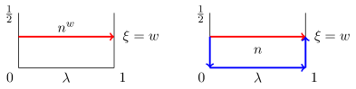
Figure 1: Graphical representations of both traditional (left) and generalized adiabatic connections (right) for a two-state ensemble. See text for further details.

$${E}^{w}_{\rm xc}[n] = \int^{1}_{0}{\rm d}\lambda\,\frac{{\rm d}F^{\lambda,w}[n]}{{\rm d}\lambda}-E_{\rm H}[n]$$ (21)

$$= \int^{1}_{0}{\rm d}\lambda\,\left[\frac{{\rm d}F^{\lambda,0}[n]}{{\rm d}\lambda}+\int_{0}^{w}{\rm d}\xi\,\frac{{\rm d}^{2}F^{\lambda,\xi}[n]}{{\rm d}\xi{\rm d}\lambda}\right]-E_{\rm H}[n]$$

$$= {E}_{\rm xc}[n]+\int_{0}^{w}{\rm d}\xi\,\left(\frac{{\rm d}F^{1,\xi}[n]}{{\rm d}\xi}-\frac{{\rm d}F^{0,\xi}[n]}{{\rm d}\xi}\right),$$

where the partially-interacting GOK functional equals along the GACE

$$F^{\lambda,\xi}[n] = (1-\xi)\,\langle\Psi^{\lambda,\xi}_{1}|\hat{T}+\lambda\hat{W}_{\rm ee}|\Psi^{\lambda,\xi}_{1}\rangle+\xi\,\langle\Psi^{\lambda,\xi}_{2}|\hat{T}+\lambda\hat{W}_{\rm ee}|\Psi^{\lambda,\xi}_{2}\rangle.$$ (22)

Since, according to Appendix 7,

$$\displaystyle\frac{{\rm d}F^{\lambda,\xi}[n]}{{\rm d}\xi} = \mathcal{E}^{\lambda,\xi}_{2}-\mathcal{E}^{\lambda,\xi}_{1},$$ (23)

we finally obtain

$${E}^{w}_{\rm xc}[n] = {E}_{\rm xc}[n]+\int_{0}^{w}{\rm d}\xi\,\Bigg{[}\Big{(}\mathcal{E}^{1,\xi}_{2}-\mathcal{E}^{1,\xi}_{1}\Big{)}-\Big{(}\mathcal{E}^{0,\xi}_{2}-\mathcal{E}^{0,\xi}_{1}\Big{)}\Bigg{]}.$$ (24)

The exact deviation of the ensemble exchange–correlation energy from the ground-state one is therefore obtained by integrating the difference in excitation energies

$$\Delta_{\rm xc}^{\xi}[n]=\Big{(}\mathcal{E}^{1,\xi}_{2}-\mathcal{E}^{1,\xi}_{1}\Big{)}-\Big{(}\mathcal{E}^{0,\xi}_{2}-\mathcal{E}^{0,\xi}_{1}\Big{)}$$ (25)

between the physical and non-interacting GOK systems over the weight interval $[0,w]$ while keeping the ensemble density fixed. Equivalently, $\Delta_{\rm xc}^{\xi}[n]$ is the first-order derivative of the ensemble exchange–correlation energy:

$$\Delta_{\rm xc}^{\xi}[n]=\frac{{\rm d}{E}^{\xi}_{\rm xc}[n]}{{\rm d}\xi}.$$ (26)

According to Eqs. (24) and (25), the ensemble exchange–correlation energy can be expanded through second order in $w$ as follows,

$${E}^{w}_{\rm xc}[n] = {E}_{\rm xc}[n]+w\Delta_{\rm xc}^{0}[n]+\frac{w^{2}}{2}\left.\frac{{\rm d}\Delta_{\rm xc}^{\xi}[n]}{{\rm d}\xi}\right|_{\xi=0}+\mathcal{O}(w^{3}),$$ (27)

where the first-order Taylor expansion coefficient

$$\Delta_{\rm xc}^{0}[n]=\Big{(}\mathcal{E}^{1,0}_{2}-\mathcal{E}^{1,0}_{1}\Big{)}-\Big{(}\mathcal{E}^{0,0}_{2}-\mathcal{E}^{0,0}_{1}\Big{)}$$ (28)

can be rewritten more explicitly as

$$\Delta_{\rm xc}^{0}[n]=\Big{(}E_{2}[n]-E_{1}[n]\Big{)}-\Big{(}\varepsilon^{0}_{2}[n]-\varepsilon^{0}_{1}[n]\Big{)},$$ (29)

where, for convenience, the first excitation in the non-interacting KS system (to which the GOK system reduces for $\xi=0$) is assumed to be a single excitation. The corresponding excitation energy $\mathcal{E}^{0,0}_{2}-\mathcal{E}^{0,0}_{1}$ is then equal to the HOMO-LUMO gap $\varepsilon^{0}_{2}[n]-\varepsilon^{0}_{1}[n]$ in the KS system whose ground-state density equals $n$. In case of multiple excitations the excitation energy would simply be written as the sum of KS orbital energy differences. On the other hand, the first excitation energy $\mathcal{E}^{1,0}_{2}-\mathcal{E}^{1,0}_{1}$ in the fully-interacting system whose ground-state density equals $n$ is simply denoted $E_{2}[n]-E_{1}[n]$.

Note that, in the particular case where $n$ equals the exact ground-state density $n^{0}=n_{\tilde{\Psi}_{1}}$ of the true physical system that is described by the Schrödinger Eq. (1), the exact excitation energy $E_{2}-E_{1}$ and the conventional KS HOMO-LUMO gap $\varepsilon^{0}_{2}-\varepsilon^{0}_{1}$ are recovered, leading thus to

$$\Delta_{\rm xc}^{0}[n^{0}]=\Big{(}E_{2}-E_{1}\Big{)}-\Big{(}\varepsilon^{0}_{2}-\varepsilon^{0}_{1}\Big{)}.$$ (30)

Levy [6] has shown that the term on the left-hand side of Eq. (30) can be interpreted as a discontinuous change in the exchange–correlation potential as $w\rightarrow 0$. For that reason we will refer to $\Delta_{\rm xc}^{\xi}[n]$ as the exchange–correlation derivative discontinuity (DD) density functional in the following.

Let us now focus on the second-order Taylor expansion coefficient in Eq. (27). Since, according to Eq. (17) and the Hellmann–Feynman theorem,

$$\frac{{\rm d}\mathcal{E}_{i}^{\lambda,\xi}}{{\rm d}\xi}=\int{\rm d}{\bf r}\,\frac{\partial v^{\lambda,\xi}({\bf r})}{\partial\xi}\,{n}_{\Psi^{\lambda,\xi}_{i}}({\bf r}),\hskip 11.38092pti=1,2,$$ (31)

the first-order derivative of the exchange–correlation DD functional can be expressed, according to Eq. (25), as

$$\left.\frac{{\rm d}\Delta_{\rm xc}^{\xi}[n]}{{\rm d}\xi}\right|_{\xi=0} = \int{\rm d}{\bf r}\,\left.\frac{\partial v^{1,\xi}({\bf r})}{\partial\xi}\right|_{\xi=0}\,\Big{(}{n}_{\Psi^{1,0}_{2}}({\bf r})-{n}_{\Psi^{1,0}_{1}}({\bf r})\Big{)}$$ (32)

$$-\int{\rm d}{\bf r}\,\left.\frac{\partial v^{0,\xi}({\bf r})}{\partial\xi}\right|_{\xi=0}\,\Big{(}{n}_{\Psi^{0,0}_{2}}({\bf r})-{n}_{\Psi^{0,0}_{1}}({\bf r})\Big{)}.$$

With the notations of Eqs. (6) and (8), the first excited states of the fully-interacting ($\Psi^{1,0}_{2}$) and KS ($\Psi^{0,0}_{2}$) systems whose ground-state densities equal $n$ simply correspond to $\Psi^{0}_{2}[n]$ and $\Phi^{0}_{2}[n]$, respectively. As ${n}_{\Psi^{1,0}_{1}}={n}_{\Psi^{0,0}_{1}}=n$, according to the density constraint in Eq. (18), we obtain

$$\left.\frac{{\rm d}\Delta_{\rm xc}^{\xi}[n]}{{\rm d}\xi}\right|_{\xi=0} = \int{\rm d}{\bf r}\,\left.\frac{\partial v^{1,\xi}({\bf r})}{\partial\xi}\right|_{\xi=0}\,\Big{(}{n}_{\Psi^{0}_{2}[n]}({\bf r})-{n}({\bf r})\Big{)}$$ (33)

$$-\int{\rm d}{\bf r}\,\left.\frac{\partial v^{0,\xi}({\bf r})}{\partial\xi}\right|_{\xi=0}\,\Big{(}{n}_{\Phi^{0}_{2}[n]}({\bf r})-{n}({\bf r})\Big{)}.$$

Moreover, as shown in Appendix 8, the fully-interacting and GOK local potentials are connected as follows

$$v^{0,\xi}({\bf r})=v^{1,\xi}({\bf r})+\frac{\delta{E}^{\xi}_{\rm Hxc}}{\delta n({\bf r})}[n],$$ (34)

which leads to the final expression

$$\left.\frac{{\rm d}\Delta_{\rm xc}^{\xi}[n]}{{\rm d}\xi}\right|_{\xi=0} = \int{\rm d}{\bf r}\,\left.\frac{\partial}{\partial\xi}\frac{\delta{E}^{\xi}_{\rm xc}}{\delta n({\bf r})}[n]\right|_{\xi=0}\,\Big{(}{n}({\bf r})-{n}_{\Psi^{0}_{2}[n]}({\bf r})\Big{)}$$ (35)

$$+\int{\rm d}{\bf r}\,\left.\frac{\partial v^{0,\xi}({\bf r})}{\partial\xi}\right|_{\xi=0}\,\Big{(}{n}_{\Psi^{0}_{2}[n]}({\bf r})-{n}_{\Phi^{0}_{2}[n]}({\bf r})\Big{)},$$

or, equivalently, according to Eq. (26),

$$\left.\frac{{\rm d}\Delta_{\rm xc}^{\xi}[n]}{{\rm d}\xi}\right|_{\xi=0} = \int{\rm d}{\bf r}\,\frac{\delta{\Delta}^{0}_{\rm xc}}{\delta n({\bf r})}[n]\,\Big{(}{n}({\bf r})-{n}_{\Psi^{0}_{2}[n]}({\bf r})\Big{)}$$ (36)

$$+\int{\rm d}{\bf r}\,\left.\frac{\partial v^{0,\xi}({\bf r})}{\partial\xi}\right|_{\xi=0}\,\Big{(}{n}_{\Psi^{0}_{2}[n]}({\bf r})-{n}_{\Phi^{0}_{2}[n]}({\bf r})\Big{)}.$$

Note that the Hartree density-functional potential does not appear in the first term on the right-hand side of Eq. (35) since the ensemble Hartree density-functional energy is weight-independent (see Eq. (19)). In addition, in the particular case where $n$ equals the exact ground-state density $n^{0}$ of the true physical system, Eq. (36) becomes

$$\left.\frac{{\rm d}\Delta_{\rm xc}^{\xi}[n^{0}]}{{\rm d}\xi}\right|_{\xi=0} = \int{\rm d}{\bf r}\,\frac{\delta\Delta^{0}_{\rm xc}}{\delta n({\bf r})}[n^{0}]\,\Big{(}{n^{0}}({\bf r})-{n}_{\tilde{\Psi}_{2}}({\bf r})\Big{)}$$ (37)

$$+\int{\rm d}{\bf r}\,\left.\frac{\partial v_{\rm s}^{\xi}[n^{0}]({\bf r})}{\partial\xi}\right|_{\xi=0}\,\Big{(}{n}_{\tilde{\Psi}_{2}}({\bf r})-{n}_{\tilde{\Phi}^{0}_{2}}({\bf r})\Big{)},$$

where $\tilde{\Psi}_{2}$ and $\tilde{\Phi}^{0}_{2}$ are the first excited states of the physical and KS systems, respectively (see Eqs. (1) and (2.1)). For clarity the local GOK potential for which the ensemble density remains equal to the exact ground-state density $n^{0}$ as the weight of the ensemble varies in the vicinity of $\xi=0$ has been denoted $v_{\rm s}^{\xi}[n^{0}]$. As shown in the next section, the Taylor expansion we obtained within the GACE for the ensemble exchange–correlation energy leads to stringent constraints on the functional.

2.4 Exact ensemble and excitation energies

Let us consider the GACE in the particular case where the density $n$ equals the exact ensemble density $n^{w}$ of the physical system. According to Eqs. (1) and (2.1), the local potentials $v^{1,w}({\bf r})$ and $v^{0,w}({\bf r})$ correspond then to the nuclear $v_{\rm ne}({\bf r})$ and GOK $v_{\rm ne}({\bf r})+\delta{E}^{w}_{\rm Hxc}[n^{w}]/\delta n({\bf r})$ potentials, respectively. Consequently, the fully-interacting excitation energy becomes the true physical one $E_{2}-E_{1}$, while the non-interacting excitation energy is the GOK one obtained from Eq. (2.1), leading thus to the following expression for the ensemble exchange–correlation DD energy:

$$\Delta_{\rm xc}^{w}[n^{w}]=E_{2}-E_{1}-\Big{(}\mathcal{E}^{w}_{{\rm s},2}-\mathcal{E}^{w}_{{\rm s},1}\Big{)}.$$ (38)

When the first excitation in the GOK system corresponds to a single excitation, the corresponding excitation energy can be rewritten as an orbital energy difference

$$\mathcal{E}^{w}_{{\rm s},2}-\mathcal{E}^{w}_{{\rm s},1}=\varepsilon_{2}^{w}-\varepsilon_{1}^{w},$$ (39)

and, consequently, the expression of Gross et al. [5] for the exact first excitation energy is recovered:

$$\displaystyle E_{2}-E_{1} = \varepsilon_{2}^{w}-\varepsilon_{1}^{w}+\Delta_{\rm xc}^{w}[n^{w}]$$ (40)

$$= \left.\varepsilon_{2}^{w}-\varepsilon_{1}^{w}+\frac{{\rm d}E_{\rm xc}^{\xi}[n^{w}]}{{\rm d}\xi}\right|_{\xi=w}.$$

It becomes clear from Eq. (40) that the weight-dependent exchange–correlation DD density functional $\Delta_{\rm xc}^{w}[n]$ plays a crucial role in the calculation of excitation energies in GOK-DFT.

In the rest of this work we will show how the GACE could be used for the development of ensemble DFAs. Before, let us mention that stringent constraints on the density functional $\Delta_{\rm xc}^{w}[n]$ can be derived from Eq. (40) when rewriting, according to Eq. (3), the excitation energy as the first-order derivative of the ensemble energy with respect to the ensemble weight $w$:

$$\frac{{\rm d}{E}^{w}}{{\rm d}w}=E_{2}-E_{1},\hskip 17.07182pt0\leq w\leq\frac{1}{2}.$$ (41)

In the exact theory this derivative should therefore not vary with $w$ or, equivalently, the ensemble energy should have no curvature:

$$\frac{{\rm d}^{k}{E}^{w}}{{\rm d}w^{k}}=0,\hskip 17.07182pt0\leq w\leq\frac{1}{2},\hskip 17.07182ptk\geq 2.$$ (42)

Note that differentiability with respect to the ensemble weight $w$ will be assumed (but it is in principle not guaranteed) for individual terms on the right-hand side of Eq. (40).

For the purpose of constructing ensemble DFAs from regular ground-state DFAs, as proposed by Nagy [36] and Paragi et al. [25, 24], Eqs. (41) and (42) should be taken in the $w=0$ limit. Here we will consider derivatives through second order only ($k=2$), which leads to the two exact conditions

$$\left.\frac{{\rm d}{E}^{w}}{{\rm d}w}\right|_{w=0}=E_{2}-E_{1},$$ (43)

and

$$\left.\frac{{\rm d}^{2}{E}^{w}}{{\rm d}w^{2}}\right|_{w=0}=0.$$ (44)

Since, according to Eq. (4), the ensemble exchange–correlation DD energy is expanded through first order as

$$\displaystyle\Delta_{\rm xc}^{w}[n^{w}] = \Delta_{\rm xc}^{w}[n^{0}]+\int{\rm d}{\bf r}\,\frac{\delta\Delta_{\rm xc}^{w}}{\delta n({\bf r})}[n^{0}]\Big{(}n^{w}({\mathbf{r}})-n^{0}({\mathbf{r}})\Big{)}+\mathcal{O}(w^{2})$$ (45)

$$= \Delta_{\rm xc}^{0}[n^{0}]+w\Bigg{(}\left.\frac{{\rm d}\Delta_{\rm xc}^{\xi}[n^{0}]}{{\rm d}\xi}\right|_{\xi=0}+\int{\rm d}{\bf r}\,\frac{\delta\Delta_{\rm xc}^{0}}{\delta n({\bf r})}[n^{0}]\Big{(}n_{\tilde{\Psi}_{2}}({\mathbf{r}})-n^{0}({\mathbf{r}})\Big{)}\Bigg{)}$$

$$+\mathcal{O}(w^{2}),$$

which gives, according to Eq. (37),

$$\displaystyle\Delta_{\rm xc}^{w}[n^{w}] = \Delta_{\rm xc}^{0}[n^{0}]+w\int{\rm d}{\bf r}\,\left.\frac{\partial v_{\rm s}^{\xi}[n^{0}]({\bf r})}{\partial\xi}\right|_{\xi=0}\,\Big{(}{n}_{\tilde{\Psi}_{2}}({\bf r})-{n}_{\tilde{\Phi}^{0}_{2}}({\bf r})\Big{)}+\mathcal{O}(w^{2}),$$ (46)

we obtain through first order, from Eqs. (40) and (41),

$$\frac{{\rm d}{E}^{w}}{{\rm d}w}=\Big{(}\varepsilon^{0}_{2}-\varepsilon^{0}_{1}\Big{)}+\Delta_{\rm xc}^{0}[n^{0}]$$

$$+w\Bigg{[}\left.\frac{{\rm d}}{{\rm d}w}\Big{(}\varepsilon_{2}^{w}-\varepsilon_{1}^{w}\Big{)}\right|_{w=0}+\int{\rm d}{\bf r}\,\left.\frac{\partial v_{\rm s}^{\xi}[n^{0}]({\bf r})}{\partial\xi}\right|_{\xi=0}\,\Big{(}{n}_{\tilde{\Psi}_{2}}({\bf r})-{n}_{\tilde{\Phi}^{0}_{2}}({\bf r})\Big{)}\Bigg{]}$$

$$+\mathcal{O}(w^{2}).$$ (47)

Eq. (30) is thus recovered from Eq. (43) while the second constraint in Eq. (44) leads to

$$\left.\frac{{\rm d}}{{\rm d}w}\Big{(}\varepsilon_{2}^{w}-\varepsilon_{1}^{w}\Big{)}\right|_{w=0}=-\int{\rm d}{\bf r}\,\left.\frac{\partial v_{\rm s}^{\xi}[n^{0}]({\bf r})}{\partial\xi}\right|_{\xi=0}\,\Big{(}{n}_{\tilde{\Psi}_{2}}({\bf r})-{n}_{\tilde{\Phi}^{0}_{2}}({\bf r})\Big{)}.$$ (48)

By rewriting the derivative on the left-hand side of Eq. (48), according to the Hellmann–Feynman theorem and Eqs. (2.1) and (39), as

$$\left.\frac{{\rm d}}{{\rm d}w}\Big{(}\varepsilon_{2}^{w}-\varepsilon_{1}^{w}\Big{)}\right|_{w=0} = \left\langle\tilde{\Phi}_{2}^{0}\left|\left.\frac{{\rm d}}{{\rm d}w}\hat{{V}}^{w}_{\rm Hxc}[n^{w}]\right|_{w=0}\right|\tilde{\Phi}_{2}^{0}\right\rangle$$ (49)

$$-\left\langle\tilde{\Phi}_{1}^{0}\left|\left.\frac{{\rm d}}{{\rm d}w}\hat{{V}}^{w}_{\rm Hxc}[n^{w}]\right|_{w=0}\right|\tilde{\Phi}_{1}^{0}\right\rangle$$

$$= \int{\rm d}{\mathbf{r}}\,\left.\frac{{\rm d}}{{\rm d}w}\frac{\delta E_{\rm Hxc}^{w}}{\delta n({\mathbf{r}})}[n^{w}]\right|_{w=0}\Big{(}n_{\tilde{\Phi}^{0}_{2}}({\mathbf{r}})-n^{0}({\mathbf{r}})\Big{)},$$

and using

$$\left.\frac{{\rm d}}{{\rm d}w}\frac{\delta E_{\rm Hxc}^{w}}{\delta n({\mathbf{r}})}[n^{w}]\right|_{w=0} = \left.\frac{\partial}{\partial w}\frac{\delta{E}^{w}_{\rm xc}}{\delta n({\bf r})}[n^{0}]\right|_{w=0}$$ (50)

$$+\int{\rm d}{\bf r^{\prime}}\,K_{\rm Hxc}({\bf r^{\prime}},{\bf r})\Big{(}n_{\tilde{\Psi}_{2}}({\mathbf{r}^{\prime}})-n^{0}({\mathbf{r}^{\prime}})\Big{)},$$

where $K_{\rm Hxc}({\bf r^{\prime}},{\bf r})=\delta^{2}E_{\rm Hxc}[n^{0}]/\delta n({\mathbf{r}^{\prime}})\delta n({\mathbf{r}})$ denotes the ground-state Hxc kernel, we conclude from Eq. (48) that the exact constraint in Eq. (44) is equivalent to

$$\int{\rm d}{\mathbf{r}}\,\frac{\delta\Delta^{0}_{\rm xc}}{\delta n({\mathbf{r}})}[n^{0}]\Big{(}n_{\tilde{\Phi}^{0}_{2}}({\mathbf{r}})-n^{0}({\mathbf{r}})\Big{)}$$

$$+\int\int{\rm d}{\bf r}{\rm d}{\bf r^{\prime}}\,K_{\rm Hxc}({\bf r^{\prime}},{\bf r})\Big{(}n_{\tilde{\Psi}_{2}}({\mathbf{r}^{\prime}})-n^{0}({\mathbf{r}^{\prime}})\Big{)}\Big{(}n_{\tilde{\Phi}^{0}_{2}}({\mathbf{r}})-n^{0}({\mathbf{r}})\Big{)}$$

$$=-\int{\rm d}{\bf r}\,\left.\frac{\partial v_{\rm s}^{\xi}[n^{0}]({\bf r})}{\partial\xi}\right|_{\xi=0}\,\Big{(}{n}_{\tilde{\Psi}_{2}}({\bf r})-{n}_{\tilde{\Phi}^{0}_{2}}({\bf r})\Big{)}.$$ (51)

Note that, when simplifying the Hartree contribution only in Eq. (50), relation (2.4) can alternatively be rewritten as

$$-\int{\rm d}{\mathbf{r}}\,\left.\frac{{\rm d}}{{\rm d}w}\frac{\delta E_{\rm xc}^{w}}{\delta n({\mathbf{r}})}[n^{w}]\right|_{w=0}\Big{(}n_{\tilde{\Phi}^{0}_{2}}({\mathbf{r}})-n^{0}({\mathbf{r}})\Big{)}$$ (52)

$$-\int{\rm d}{\bf r}\,\left.\frac{\partial v_{\rm s}^{\xi}[n^{0}]({\bf r})}{\partial\xi}\right|_{\xi=0}\,\Big{(}{n}_{\tilde{\Psi}_{2}}({\bf r})-{n}_{\tilde{\Phi}^{0}_{2}}({\bf r})\Big{)}$$

$$=\int{\rm d}{\bf r}\,\left(\Big{[}n_{\tilde{\Phi}^{0}_{2}}({\mathbf{r}})-n^{0}({\mathbf{r}})\Big{]}\int{\rm d}{\bf r^{\prime}}\,\frac{\Big{[}n_{\tilde{\Psi}_{2}}({\mathbf{r}^{\prime}})-n^{0}({\mathbf{r}^{\prime}})\Big{]}}{|{\mathbf{r}}-{\mathbf{r}^{\prime}}|}\right),$$

which is nothing but Levy’s constraint (see Eq. (30) in Ref. [6]) in the $w\rightarrow 0$ limit. Interestingly, we obtain in the second integral on the left-hand side of Eq. (52) an explicit expression for the contribution that arises from the discontinuous change of the exchange–correlation potential as $w\rightarrow 0$. Note that this contribution comes directly from the GACE, where the ensemble density of the non-interacting system is held fixed to the ground-state density $n^{0}$ while the ensemble weight varies in the vicinity of $\xi=0$.

Returning to the formulation in Eq. (2.4), an accurate value for the integral on the right-hand side could in principle be obtained when constructing the GACE with ab initio methods, as discussed further in Sec. 2.5. The contributions on the left-hand side of Eq. (2.4) can, on the other hand, be computed with DFAs. The stringent constraint we derived could thus be used for developing DFAs to $\Delta^{0}_{\rm xc}[n]$. Interestingly the ground-state kernel, that plays a key role in TD-DFT [1], appears in the derivation of the excitation energy within GOK-DFT. Connections between the two approaches should be investigated further in the light of the recent work of Ziegler and coworkers [17, 19] on constricted variational density-functional theory (CV-DFT). A formal connection might also be obtained when considering imaginary temperatures in Boltzmann factors for the ensemble weights [21]. Work is in progress in these directions.

2.5 Construction of the GACE

By analogy with traditional ground-state AC calculations [31, 32, 33], the GACE could in principle be constructed from the partially-interacting GOK functional introduced in Eq. (22). Note that the functional is defined for ensemble $v$-representable densities. The domain of the functional can be enlarged to ensemble $N$ representable densities by using a Levy–Lieb constrained-search formulation [5, 21],

$$F^{\lambda,\xi}[n] = \underset{\{\Psi_{1},\Psi_{2}\}^{\xi}\rightarrow n}{\rm min}\bigg{\{}(1-\xi)\,\langle\Psi_{1}|\hat{T}+\lambda\hat{W}_{\rm ee}|\Psi_{1}\rangle+\xi\,\langle\Psi_{2}|\hat{T}+\lambda\hat{W}_{\rm ee}|\Psi_{2}\rangle\bigg{\}},$$ (53)

where the minimization in Eq. (53) is restricted to orthonormal sets of wavefunctions $\{\Psi_{1},\Psi_{2}\}^{\xi}$ whose ensemble density $(1-\xi)\,n_{\Psi_{1}}+\xi\,n_{\Psi_{2}}$ equals $n$.

The minimizing wavefunctions $\Psi^{\lambda,\xi}_{1}$ and $\Psi^{\lambda,\xi}_{2}$ can alternatively be reached when searching for the local potential $v^{\lambda,\xi}$ that was introduced in Eq. (17). For that purpose we define, for a given local potential $v$, the partially-interacting Hamiltonian $\hat{H}^{\lambda}[v]=\hat{T}+\lambda\hat{W}_{\rm ee}+\int{\rm d}{\bf r}\,v({\bf r})\,\hat{n}({\bf r})$ and denote $\mathcal{E}^{\lambda}_{1}[v]$ and $\mathcal{E}^{\lambda}_{2}[v]$ the associated ground- and first-excited-state energies, respectively. According to the GOK variational principle,

$$(1-\xi)\,\langle\Psi^{\lambda,\xi}_{1}|\hat{H}^{\lambda}[v]|\Psi^{\lambda,\xi}_{1}\rangle+\xi\,\langle\Psi^{\lambda,\xi}_{2}|\hat{H}^{\lambda}[v]|\Psi^{\lambda,\xi}_{2}\rangle\geq(1-\xi)\mathcal{E}^{\lambda}_{1}[v]+\xi\,\mathcal{E}^{\lambda}_{2}[v],$$ (54)

or, equivalently,

$$F^{\lambda,\xi}[n]\geq(1-\xi)\mathcal{E}^{\lambda}_{1}[v]+\xi\,\mathcal{E}^{\lambda}_{2}[v]-\int{\rm d}{\bf r}\,v({\bf r})\,{n}({\bf r}).$$ (55)

The partially-interacting GOK functional can therefore be rewritten as a Legendre–Fenchel transform [38, 39, 40, 41]

$$F^{\lambda,\xi}[n]=\underset{v}{\rm sup}\bigg{\{}\mathcal{F}^{\lambda,\xi}[v,n]\bigg{\}},$$ (56)

where

$$\mathcal{F}^{\lambda,\xi}[v,n]=(1-\xi)\mathcal{E}^{\lambda}_{1}[v]+\xi\,\mathcal{E}^{\lambda}_{2}[v]-\int{\rm d}{\bf r}\,v({\bf r})\,{n}({\bf r}),$$ (57)

and the maximizing potential in Eq. (56), if it exists, equals $v^{\lambda,\xi}$. In the latter case, where we assume that the density $n$ can be represented by a non-degenerate two-state partially-interacting ensemble, expressions in Eqs. (53) and (56) are equivalent. In the special case $\xi=0$, it would therefore be assumed that the density $n$ is pure-state-$v$-representable. For any density, the ground-state Legendre–Fenchel transform recovered when $\xi=0$ is in fact equivalent to the Levy–Valone–Lieb functional [42]. Degeneracies associated with the ground-state energy $\mathcal{E}^{\lambda}_{1}[v]$ can indeed allow for the description of densities that are not pure-state-$v$-representable.

Returning to non-degenerate two-state ensemble $v$-representable densities, we note that Nagy’s AC [35] can be constructed by fixing the ensemble weight $\xi$ to a given value $w$ and by choosing the weight-dependent ensemble density $n^{w}$ as input density in Eq. (56). In this case the maximizing local potential $\tilde{v}^{\lambda,w}$ is determined from the stationary condition

$$\frac{\delta\mathcal{F}^{\lambda,w}}{\delta v(\bf r)}[\tilde{v}^{\lambda,w},n^{w}]=0.$$ (58)

On the other hand, the GACE is constructed when varying both ensemble weight and interaction strength while keeping the density fixed to $n$. The maximizing potential $v^{\lambda,\xi}$ is then obtained from the variational condition

$$\frac{\delta\mathcal{F}^{\lambda,\xi}}{\delta v(\bf r)}[{v}^{\lambda,\xi},n]=0,\hskip 11.38092pt0\leq\xi\leq w,$$ (59)

which, according to Eq. (57), is equivalent to

$$(1-\xi)\frac{\delta\mathcal{E}^{\lambda}_{1}}{\delta{v}({\bf r})}[{v}^{\lambda,\xi}]+\xi\,\frac{\delta\mathcal{E}^{\lambda}_{2}}{\delta{v}({\bf r})}[{v}^{\lambda,\xi}]={n}({\bf r}),\hskip 11.38092pt0\leq\xi\leq w.$$ (60)

Since, according to the Hellmann–Feynman theorem, each individual functional derivatives correspond to the individual densities,

$$\frac{\delta\mathcal{E}^{\lambda}_{i}}{\delta{v}({\bf r})}[{v}^{\lambda,\xi}]={n}_{\Psi_{i}^{\lambda,\xi}}({\bf r}),\hskip 11.38092pt\hskip 5.69046pti=1,2,$$ (61)

the density constraint in Eq. (18) is recovered from Eq. (60).

Let us consider the particular case where the input density $n$ equals $n^{w}$. In contrast to Nagy’s AC, the variational condition in Eq. (59) will be fulfilled along the GACE for any value of the ensemble weight in the range $0\leq\xi\leq w$,

$$\frac{\delta\mathcal{F}^{\lambda,\xi}}{\delta v(\bf r)}[{v}^{\lambda,\xi},n^{w}]=0.$$ (62)

Nagy’s AC is simply recovered when $\xi=w$. In this case ${v}^{\lambda,\xi}$ reduces to the local potential $\tilde{v}^{\lambda,w}$ introduced in Eq. (58).

The GACE could in principle be computed along those lines by using ab initio methods for the description of the partially-interacting ensemble. For that purpose, the recent work of Teale et al. [31, 32, 33] on the computation of ground-state ACs should be extended to ensembles. Such an approach would provide precious data for the development of ensemble DFAs.

Let us finally stress that the GACE offers some flexibility in the choice of the input density. For convenience, one may wish to construct a GACE where the local potential ${v}^{\lambda,\xi}$ does not depend on the ensemble weight $\xi$. Consequently, individual densities of the ground- and first-excited states in the partially-interacting system would be weight-independent. Since the ensemble density is fixed along the GACE, it would simply mean that the individual densities are equal. As an illustration, we propose in the following to construct such a GACE analytically for the simple H₂ model system in a minimal basis.

3 Analytical derivation of the GACE for H₂ in a minimal basis

We consider in this section the H₂ molecule in a Slater minimal basis consisting of the $1s_{A}$ and $1s_{B}$ atomic orbitals localized on the left and right hydrogen atoms, respectively [43, 44]. The basis functions are identical with $\zeta=1$. For large bond distances the bonding and anti-bonding molecular orbitals are equal to $1\sigma_{g}=\frac{1}{\sqrt{2}}\big{(}1s_{A}+1s_{B}\big{)}$ and $1\sigma_{u}=\frac{1}{\sqrt{2}}\big{(}1s_{A}-1s_{B}\big{)}$, respectively. Both traditional AC and GACE will be constructed in the following within the ${}^{1}\Sigma_{g}^{+}$ symmetry. The space of two-electron wavefunctions to be considered reduces then to the two Slater determinants $1\sigma_{g}^{2}$ and $1\sigma_{u}^{2}$. Since these two determinants differ by a double excitation, they are not coupled by one-electron operators such as local potential operators. Even though equations are derived explicitly for H₂, any two-level system that fulfils the latter condition could be described similarly. Returning to H₂, in the dissociation limit, the two-state ensemble will therefore consists of the neutral $\frac{1}{\sqrt{2}}\big{(}1\sigma_{g}^{2}-1\sigma_{u}^{2}\big{)}$ and ionic $\frac{1}{\sqrt{2}}\big{(}1\sigma_{g}^{2}+1\sigma_{u}^{2}\big{)}$ states.

The analytical derivation of the Legendre–Fenchel transform is first presented for the ground state in Sec. 3.1. The extension to the two-state ensemble is then given in Sec. 3.2. In the light of these derivations we finally propose in Sec. 3.3 a simple DFA to the ensemble exchange–correlation functional.

3.1 AC for the ground state

Let the matrix representation of the physical fully-interacting Hamiltonian in the basis of the $1\sigma_{g}^{2}$ and $1\sigma_{u}^{2}$ determinants be

$$\left[\hat{H}\right]=\left[\begin{array}[]{c c}E_{g}&K\\ K&E_{u}\end{array}\right],$$ (65)

where

$$E_{i}=\langle 1\sigma_{i}^{2}|\hat{T}+\hat{W}_{\rm ee}+\hat{V}_{\rm ne}|1\sigma_{i}^{2}\rangle,\hskip 11.38092pti=g,u,$$

$$K=\langle 1\sigma_{g}^{2}|\hat{W}_{\rm ee}|1\sigma_{u}^{2}\rangle.$$ (66)

The ground-state wavefunction $\Psi_{1}$ and ground-state energy $E_{1}$ are obtained by diagonalizing $\left[\hat{H}\right]$, which leads to

$$E_{1}=\frac{1}{2}\left({E}_{g}+{E}_{u}-\sqrt{\big{(}{E}_{g}-{E}_{u}\big{)}^{2}+4K^{2}}\right),$$ (67)

and

$$|{\Psi}_{1}\rangle=\frac{1}{\sqrt{1+C_{u}^{2}}}\Big{(}|1\sigma_{g}^{2}\rangle+C_{u}|1\sigma_{u}^{2}\rangle\Big{)},$$ (68)

with

$$C_{u}=\frac{E_{1}-E_{g}}{K}.$$ (69)

Since $1\sigma_{g}^{2}$ and $1\sigma_{u}^{2}$ differ by a double excitation, they are not coupled by the density operator. Hence the ground-state density can be expressed as

$$n^{0}({\bf r})=\langle{\Psi}_{1}|\hat{n}({\bf r})|{\Psi}_{1}\rangle=\frac{1}{1+C_{u}^{2}}\Big{(}n_{g}({\bf r})+C_{u}^{2}\,n_{u}({\bf r})\Big{)},$$ (70)

where $n_{g}$ and $n_{u}$ denote the densities associated with the $1\sigma_{g}^{2}$ and $1\sigma_{u}^{2}$ determinants, respectively.

Before constructing the AC for the ground-state density $n^{0}$, let us first mention that the HK theorem may not be fulfilled in a finite basis [45, 46]. Here a non-interacting Hamiltonian $\hat{H}^{0}=\hat{T}+\int{\rm d}{\bf r}\,v({\bf r})\,\hat{n}({\bf r})$ will simply be represented by a diagonal matrix since the local potential operator does not couple the $1\sigma_{g}^{2}$ and $1\sigma_{u}^{2}$ determinants:

$$\left[\hat{H}^{0}\right]=\left[\begin{array}[]{c c}\langle 1\sigma_{g}^{2}|\hat{T}|1\sigma_{g}^{2}\rangle+V_{g}&0\\ 0&\langle 1\sigma_{u}^{2}|\hat{T}|1\sigma_{u}^{2}\rangle+V_{u}\end{array}\right],$$ (73)

where the two matrix elements $V_{g}$ and $V_{u}$ defined as

$$V_{i}=\int{\rm d}{\bf r}\,v({\bf r})\,{n}_{i}({\bf r}),\hskip 11.38092pti=g,u,$$ (74)

fully determine the potential in the minimal basis. In the particular case where the density $n_{g}$ is considered, the KS local potential is obviously not unique since the ground state of the non-interacting system remains equal to the $1\sigma_{g}^{2}$ determinant as long as the following condition is fulfilled

$$V_{g}-V_{u}<\langle 1\sigma_{u}^{2}|\hat{T}|1\sigma_{u}^{2}\rangle-\langle 1\sigma_{g}^{2}|\hat{T}|1\sigma_{g}^{2}\rangle.$$ (75)

On the other hand, the ground-state density $n^{0}$ is a linear combination of $n_{g}$ and $n_{u}$. Consequently, the KS $1\sigma_{g}^{2}$ and $1\sigma_{u}^{2}$ determinants must be degenerate so that the non-interacting density equals the interacting one. In other words an ensemble is required in the minimal basis while, in larger basis sets and for a finite bond distance, it is not (see, for example, Ref. [31]). This will be discussed further in the following. The KS potential is therefore uniquely defined (up to a constant) in the minimal basis by the equality

$$V^{0}_{g}-V^{0}_{u}=\langle 1\sigma_{u}^{2}|\hat{T}|1\sigma_{u}^{2}\rangle-\langle 1\sigma_{g}^{2}|\hat{T}|1\sigma_{g}^{2}\rangle.$$ (76)

It is then relevant to construct an AC for the ground-state density within the minimal basis. For that purpose we introduce the matrix representation of the partially-interacting Hamiltonian

$$\left[\hat{H}^{\lambda}\right]=\left[\begin{array}[]{c c}\langle 1\sigma_{g}^{2}|\hat{T}+\lambda\hat{W}_{\rm ee}|1\sigma_{g}^{2}\rangle+V_{g}&\lambda K\\ \lambda K&\langle 1\sigma_{u}^{2}|\hat{T}+\lambda\hat{W}_{\rm ee}|1\sigma_{u}^{2}\rangle+V_{u}\end{array}\right],$$ (79)

and, for convenience, substitute the parameters $\mathcal{V}_{g}$ and $\mathcal{V}_{u}$ for $V_{g}$ and $V_{u}$, respectively, where

$${V}_{i}=\lambda E_{i}-\langle 1\sigma_{i}^{2}|\hat{T}+\lambda\hat{W}_{\rm ee}|1\sigma_{i}^{2}\rangle+\lambda\mathcal{V}_{i},\hskip 11.38092pti=g,u.$$ (80)

Note that one single parameter

$$\upsilon=\mathcal{V}_{g}-\mathcal{V}_{u}$$ (81)

is in fact sufficient, since the local potential is determined up to a constant. This leads to the following parameterization of the partially-interacting Hamiltonian

$$\left[\hat{H}^{\lambda}\right]=\lambda\left[\begin{array}[]{c c}E_{g}+\upsilon&K\\ K&E_{u}\end{array}\right]+\lambda\mathcal{V}_{u}.$$ (84)

Note that, within this parameterization, the degeneracy of the KS determinants is ensured for $\lambda=0$.

The ground-state Legendre–Fenchel transform, from which we will construct the AC for the ground-state density $n^{0}$, is obtained as follows [38, 39, 40]

$$F^{\lambda}[n^{0}]=\underset{\upsilon}{\rm sup}\bigg{\{}\mathcal{F}^{\lambda}[\upsilon,n^{0}]\bigg{\}},$$ (85)

where, according to Eqs. (70) and (74),

$$\mathcal{F}^{\lambda}[\upsilon,n^{0}] = \mathcal{E}^{\lambda}_{1}(\upsilon)-\int{\rm d}{\bf r}\,v({\bf r})\,{n}^{0}({\bf r}),$$ (86)

$$= \mathcal{E}^{\lambda}_{1}(\upsilon)-\frac{1}{1+C_{u}^{2}}\Big{(}V_{g}+C_{u}^{2}V_{u}\Big{)},$$

and, according to Eq. (84), the auxiliary ground-state energy equals

$$\mathcal{E}^{\lambda}_{1}(\upsilon)=\frac{\lambda}{2}\left({E}_{g}+\upsilon+{E}_{u}-\sqrt{\big{(}{E}_{g}+\upsilon-{E}_{u}\big{)}^{2}+4K^{2}}\right)+\lambda\mathcal{V}_{u}.$$ (87)

Since in our parameterization $\mathcal{V}_{u}$ is a constant, $V_{u}$ does not vary with $\upsilon$ and

$$\frac{{\rm d}V_{g}}{{\rm d}\upsilon}=\lambda,$$ (88)

according to Eqs. (80) and (81). The maximizing parameter $\upsilon^{\lambda}$ in Eq. (85) is therefore obtained when solving

$$\frac{{\rm d}}{{\rm d}\upsilon}\mathcal{F}^{\lambda}[\upsilon,n^{0}] = \frac{{\rm d}\mathcal{E}^{\lambda}_{1}(\upsilon)}{{\rm d}\upsilon}-\frac{\lambda}{1+C_{u}^{2}}=0,$$ (89)

which, according to Appendix 9, leads to the unique solution

$$\upsilon^{\lambda}=0,\hskip 11.38092pt0\leq\lambda\leq 1,$$ (90)

or, equivalently,

$$V^{\lambda}_{g}-V^{\lambda}_{u}=\langle 1\sigma_{u}^{2}|\hat{T}-\lambda[\hat{T}+\hat{V}_{\rm ne}]|1\sigma_{u}^{2}\rangle-\langle 1\sigma_{g}^{2}|\hat{T}-\lambda[\hat{T}+\hat{V}_{\rm ne}]|1\sigma_{g}^{2}\rangle.$$ (91)

We thus conclude from Eq. (84) that the ground-state AC can simply be constructed in the minimal basis when multiplying the fully-interacting Hamiltonian by the interaction strength $\lambda$:

$$\left[\hat{H}^{\lambda}\right]=\lambda\left[\hat{H}\right]+\lambda\mathcal{V}_{u},$$ (92)

which means that the ground-state wavefunction does not vary along the AC,

$$\Psi_{1}^{\lambda}=\Psi_{1},\hskip 11.38092pt0\leq\lambda\leq 1.$$ (93)

Note that the description in the minimal basis of the physical ground-state wavefunction of H₂ becomes exact in the dissociation limit. For dissociated systems, the Legendre–Fenchel transform will however be ill-defined in the sense that the functional derivative of the energy with respect to the electron density does not exist [47]. Let us therefore stress that what is described here is the near dissociation of H₂ when neglecting the overlap between $1s_{A}$ and $1s_{B}$ orbitals.

According to Eq. (93), when approaching the dissociation limit, the exact value for the ground-state Hxc integrand $\langle\Psi_{1}^{\lambda}|\hat{W}_{\rm ee}|\Psi_{1}^{\lambda}\rangle$ should therefore be expected to become independent on the interaction strength $\lambda$. This was observed numerically by Teale et al. [31] An important difference though between their calculations, which were performed in large basis sets, and the analytical ones presented here lies in the fact that, in the $\lambda$=0 limit, Teale et al. [31] obtain a single determinantal KS wavefunction while we need to use an ensemble of two states to reproduce the ground-state density. Consequently, the large increase in the integrand curvature that Teale et al. observed for large bond distances when approaching the $\lambda$=0 limit cannot be reproduced in the minimal basis.

Let us finally mention that, by applying Nagy’s formula in Eq. (16) for $w=0$ and using Eq. (93), we obtain the following expression for the ground-state exchange–correlation energy

$$E_{\rm xc}[n^{0}] = \int^{1}_{0}{\rm d}{\lambda}\,\langle\Psi_{1}^{\lambda}|\hat{W}_{\rm ee}|\Psi_{1}^{\lambda}\rangle-E_{\rm H}[n^{0}]$$ (94)

$$= \langle\Psi_{1}|\hat{W}_{\rm ee}|\Psi_{1}\rangle-E_{\rm H}[n^{0}],$$

which gives, in the dissociation limit [43, 44],

$$E_{\rm xc}[n^{0}]\underset{R\rightarrow+\infty}{\longrightarrow}-\frac{5}{8}.$$ (95)

Interestingly, since $E_{g}=E_{u}$ and $K={5}/{16}$ a.u. in the dissociation limit [43, 44], the first excitation energy $E_{2}-E_{1}$ of the physical system, where

$$E_{2}=\frac{1}{2}\left({E}_{g}+{E}_{u}+\sqrt{\big{(}{E}_{g}-{E}_{u}\big{)}^{2}+4K^{2}}\right),$$ (96)

according to Eq. (65), reduces to

$$E_{2}-E_{1}\underset{R\rightarrow+\infty}{\longrightarrow}2K=\frac{5}{8}.$$ (97)

Since the KS determinants are degenerate in the minimal basis, the non-interacting KS excitation energy in Eq. (30) equals zero and the exchange–correlation DD energy computed for the ground-state density becomes

$$\Delta_{\rm xc}^{0}[n^{0}]=E_{2}-E_{1}\underset{R\rightarrow+\infty}{\longrightarrow}-E_{\rm xc}[n^{0}].$$ (98)

3.2 ACs for the ensemble

The AC constructed in Sec. 3.1 for the ground state of H₂ in a minimal basis is also valid for the two-state ensemble $\{\Psi_{1},\Psi_{2}\}^{w}$ where

$$|{\Psi}_{2}\rangle=\frac{1}{\sqrt{1+C_{g}^{2}}}\Big{(}C_{g}|1\sigma_{g}^{2}\rangle+|1\sigma_{u}^{2}\rangle\Big{)}$$ (99)

is the physical excited state whose energy $E_{2}$ is given in Eq. (96) and

$$C_{g}=\frac{E_{2}-E_{u}}{K}.$$ (100)

Indeed, since the physical fully-interacting Hamiltonian is simply scaled by the interaction strength along the ground-state AC (see Eq. (92)), both ground and excited states do not vary with $\lambda$,

$$\Psi_{i}^{\lambda}=\Psi_{i},\hskip 11.38092pt0\leq\lambda\leq 1,\hskip 11.38092pti=1,2,$$ (101)

and the density constraint of Nagy’s AC is therefore fulfilled

$$(1-w)\,n_{\Psi_{1}^{\lambda}}({\bf r})+w\,n_{\Psi_{2}^{\lambda}}({\bf r})=(1-w)\,n_{\Psi_{1}}({\bf r})+w\,n_{\Psi_{2}}({\bf r}),\hskip 11.38092pt0\leq\lambda\leq 1.$$ (102)

Note that, due to the degeneracy of the non-interacting GOK states and according to Eq. (38), relation (98) remains fulfilled for any value of $w$:

$$\Delta_{\rm xc}^{w}[n^{w}]=E_{2}-E_{1}\underset{R\rightarrow+\infty}{\longrightarrow}-E_{\rm xc}[n^{0}].$$ (103)

Let us now discuss the construction of the GACE in the minimal basis. For simplicity, we will consider the situation where the local potential that holds the ensemble density fixed, as both ensemble weight $\xi$ and interaction strength $\lambda$ vary along the GACE, does not depend on $\xi$. In the particular case where $\lambda=1$, the fully-interacting densities of the ground and first-excited states should therefore be equal. Since, according to Eq. (99), the density of the excited state can be expressed as

$$n_{{\Psi}_{2}}({\bf r})=\langle{\Psi}_{2}|\hat{n}({\bf r})|{\Psi}_{2}\rangle=\frac{1}{1+C_{g}^{2}}\Big{(}C_{g}^{2}\,n_{g}({\bf r})+\,n_{u}({\bf r})\Big{)},$$ (104)

we deduce from Eq. (70) the following condition

$$C_{u}^{2}C_{g}^{2}-1=\Big{(}C_{u}C_{g}-1\Big{)}\Big{(}C_{u}C_{g}+1\Big{)}=0,$$ (105)

which, when combined with the inequalities $C_{g}<0$ and $C_{u}>0$, leads to

$$C_{u}C_{g}=-1.$$ (106)

Since $K>0$, we finally conclude from Eqs. (69) and (100) that the $1\sigma_{g}^{2}$ and $1\sigma_{u}^{2}$ determinants should be degenerate in the fully-interacting system:

$$E_{g}=E_{u}.$$ (107)

Consequently, the fully-interacting Hamiltonian to be used in the GACE equals

$$\left[\hat{H}^{1,\xi}\right]=\left[\begin{array}[]{c c}E_{g}&K\\ K&E_{g}\end{array}\right].$$ (110)

The corresponding weight-independent ground-state wavefunction

$$|{\Psi_{1}^{1,\xi}}\rangle=|\overline{\Psi}_{1}\rangle=\frac{1}{\sqrt{2}}\Big{(}|1\sigma_{g}^{2}\rangle-|1\sigma_{u}^{2}\rangle\Big{)},$$ (111)

whose energy equals $\mathcal{E}_{1}^{1,\xi}=E_{g}-K$, describes the neutral dissociated state of H₂ while the weight-independent excited state

$$|{\Psi_{2}^{1,\xi}}\rangle=|\overline{\Psi}_{2}\rangle=\frac{1}{\sqrt{2}}\Big{(}|1\sigma_{g}^{2}\rangle+|1\sigma_{u}^{2}\rangle\Big{)},$$ (112)

whose energy equals $\mathcal{E}_{2}^{1,\xi}=E_{g}+K$, describes the ionic state. It is then clear that the ensemble density remains fixed as the ensemble weight $\xi$ varies:

$$n({\bf r})=(1-\xi)\,n_{\Psi_{1}^{1,\xi}}({\bf r})+\xi\,\,n_{\Psi_{2}^{1,\xi}}({\bf r})=\frac{1}{2}\Big{(}n_{g}({\bf r})+n_{u}({\bf r})\Big{)}.$$ (113)

The GACE can now be constructed with the partially-interacting Hamiltonian written in Eq. (79) by substituting the variables $\overline{\mathcal{V}}_{g}$ and $\overline{\mathcal{V}}_{u}$ for $V_{g}$ and $V_{u}$, respectively, with

$${V}_{i}=\lambda E_{g}-\langle 1\sigma_{i}^{2}|\hat{T}+\lambda\hat{W}_{\rm ee}|1\sigma_{i}^{2}\rangle+\lambda\overline{\mathcal{V}}_{i},\hskip 11.38092pti=g,u,$$ (114)

which leads to the following parameterization

$$\left[\hat{H}^{\lambda}\right]=\lambda\left[\begin{array}[]{c c}E_{g}+\overline{\upsilon}&K\\ K&E_{g}\end{array}\right]+\lambda\overline{\mathcal{V}}_{u},$$ (117)

where $\overline{\upsilon}=\overline{\mathcal{V}}_{g}-\overline{\mathcal{V}}_{u}$ is the parameter than defines uniquely (up to a constant) the local potential in the minimal basis. The auxiliary ground- and excited-state energies are therefore expressed as

$$\mathcal{E}^{\lambda}_{1}(\overline{\upsilon})=\frac{\lambda}{2}\left(2{E}_{g}+\overline{\upsilon}-\sqrt{\overline{\upsilon}^{2}+4K^{2}}\right)+\lambda\overline{\mathcal{V}}_{u},$$ (118)

and

$$\mathcal{E}^{\lambda}_{2}(\overline{\upsilon})=\frac{\lambda}{2}\left(2{E}_{g}+\overline{\upsilon}+\sqrt{\overline{\upsilon}^{2}+4K^{2}}\right)+\lambda\overline{\mathcal{V}}_{u},$$ (119)

respectively. According to Eq. (56), we can thus express the Legendre–Fenchel transform for the ensemble as

$$F^{\lambda,\xi}[n]=\underset{\overline{\upsilon}}{\rm sup}\bigg{\{}\mathcal{F}^{\lambda,\xi}[\overline{\upsilon},n]\bigg{\}},$$ (120)

where, according to Eqs. (74) and (113),

$$\mathcal{F}^{\lambda,\xi}[\overline{\upsilon},n] = (1-\xi)\mathcal{E}^{\lambda}_{1}(\overline{\upsilon})+\xi\,\mathcal{E}^{\lambda}_{2}(\overline{\upsilon})-\int{\rm d}{\bf r}\,v({\bf r})\,{n}({\bf r}),$$ (121)

$$= \frac{\lambda}{2}\left(2{E}_{g}+\overline{\upsilon}+(2\xi-1)\sqrt{\overline{\upsilon}^{2}+4K^{2}}\right)+\lambda\overline{\mathcal{V}}_{u}-\frac{1}{2}\Big{(}V_{g}+V_{u}\Big{)}.$$

Since in our parameterization $\overline{\mathcal{V}}_{u}$ is a constant, $V_{u}$ does not vary with $\overline{\upsilon}$ and ${\rm d}V_{g}/{\rm d}\overline{\upsilon}=\lambda$, according to Eq. (114). Consequently, the maximizing $\overline{\upsilon}^{\lambda,\xi}$ parameter in Eq. (120) fulfills

$$\frac{{\rm d}}{{\rm d}\overline{\upsilon}}\mathcal{F}^{\lambda,\xi}[\overline{\upsilon},n] = \frac{\lambda(2\xi-1)}{2}\frac{\overline{\upsilon}}{\sqrt{\overline{\upsilon}^{2}+4K^{2}}}=0,$$ (122)

which leads to the unique solution

$$\overline{\upsilon}^{\lambda,\xi}=0,\hskip 11.38092pt0\leq\lambda\leq 1,\hskip 11.38092pt0\leq\xi\leq w,$$ (123)

or, equivalently,

$$V^{\lambda,\xi}_{g}-V^{\lambda,\xi}_{u}=\langle 1\sigma_{u}^{2}|\hat{T}+\lambda\hat{W}_{\rm ee}|1\sigma_{u}^{2}\rangle-\langle 1\sigma_{g}^{2}|\hat{T}+\lambda\hat{W}_{\rm ee}|1\sigma_{g}^{2}\rangle.$$ (124)

We thus conclude from Eq. (117) that the GACE can be constructed in the minimal basis when using the partially-interacting Hamiltonian

$$\left[\hat{H}^{\lambda,\xi}\right]=\lambda\left[\begin{array}[]{c c}E_{g}&K\\ K&E_{g}\end{array}\right]+\lambda\overline{\mathcal{V}}_{u}.$$ (127)

In this simple model both ground- and excited-state wavefunctions will therefore not vary along the GACE,

$$\Psi_{i}^{\lambda,\xi}=\overline{\Psi}_{i},\hskip 11.38092pt0\leq\lambda\leq 1,\hskip 11.38092pt0\leq\xi\leq w,\hskip 11.38092pti=1,2,$$ (128)

and the auxiliary excitation energy equals

$$\mathcal{E}_{2}^{\lambda,\xi}-\mathcal{E}_{1}^{\lambda,\xi}=2\lambda K.$$ (129)

According to Eq. (24), the ensemble exchange–correlation energy is then equal to

$${E}^{w}_{\rm xc}[n]={E}_{\rm xc}[n]+2Kw.$$ (130)

Since the density $n$ defined in Eq. (113) corresponds to the exact ground-state density $n^{0}$ in the dissociation limit of H₂, we obtain from Eqs. (95) and (97)

$${E}^{w}_{\rm xc}[n]\underset{R\rightarrow+\infty}{\longrightarrow}\Big{(}1-w\Big{)}{E}_{\rm xc}[n],$$ (131)

or, equivalently,

$${\Delta}^{w}_{\rm xc}[n]\underset{R\rightarrow+\infty}{\longrightarrow}-{E}_{\rm xc}[n].$$ (132)

3.3 The GSxc approximation

From the ensemble exchange–correlation energy expression in Eq. (131), which is exact for the dissociated H₂ molecule in a minimal basis, we deduce the following DFA for a two-state ensemble:

$${E}^{w,\mbox{\tiny DFA}}_{\rm xc}[n]=\Big{(}1-w\Big{)}{E}^{\mbox{\tiny DFA}}_{\rm xc}[n],$$ (133)

or, equivalently,

$${\Delta}^{w,\mbox{\tiny DFA}}_{\rm xc}[n]=-{E}^{\mbox{\tiny DFA}}_{\rm xc}[n],$$ (134)

where any pure ground-state exchange–correlation density functional can in principle be used. We thus define from Eq. (30) the approximate ground-state exchange–correlation energy (GSxc)-corrected excitation energy expression

$$\Big{(}E_{2}-E_{1}\Big{)}_{\rm GSxc}=\varepsilon^{0}_{2}-\varepsilon^{0}_{1}-{E}^{\mbox{\tiny DFA}}_{\rm xc}[n^{0}],$$ (135)

where the exchange–correlation energy computed for the ground-state density is subtracted from the KS orbital energy difference. Note that in case of multiple excitations the latter will be replaced by a sum of orbital energy differences.

4 Illustrative result: the $2^{1}\Sigma^{+}_{g}$ state of H₂ upon bond stretching

The first ${}^{1}\Sigma^{+}_{g}$ excitation energy in H₂ has been computed within the GSxc approximation introduced in Sec. 3.3. Comparison is made with Full Configuration Interaction (FCI) and regular TD-DFT results. The local density (LDA) [48] as well as the semi-local Perdew–Burke–Ernzerhof (PBE) [49] and 1994 Leeuwen–Baerends (LB94) [50] approximations have been considered. The large aug-cc-pVQZ basis set [51] has been used. Calculations were performed with the DALTON2011 program [52].

Regular adiabatic TD-DFT fails in describing the $2^{1}\Sigma^{+}_{g}$ excited state of H₂ upon bond stretching since, for bond distances larger than 3 a.u., this state exhibits a strong doubly-excited character [53], as shown in Fig. 2. The avoided crossing obtained at the FCI level around $R$=3 a.u. indicates the change in character for the $2^{1}\Sigma^{+}_{g}$ state, from singly [$1\sigma_{g}\rightarrow 2\sigma_{g}$] to doubly [$(1\sigma_{g})^{2}\rightarrow(1\sigma_{u})^{2}$] excited, while the TD-DFT curves remain associated with the single excitation even for large bond distances.

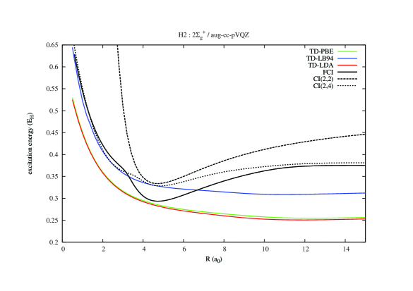
Figure 2: First ${}^{1}\Sigma_{g}^{+}$ excitation energy in H₂ along the bond-breaking coordinate obtained with regular TD-DFT (solid colored lines) and CI (black lines) methods. FCI (solid line) is compared to CI(2,2) (dashed line), where the two electrons are distributed among the $1\sigma_{g}$ and $1\sigma_{u}$ orbitals, and to CI(2,4) (dotted line) where the two electrons are distributed among the $1\sigma_{g}$, $2\sigma_{g}$, $1\sigma_{u}$ and $2\sigma_{u}$ orbitals.

Before discussing the performance of the GSxc approximation, we should first stress that the minimal basis model on which it relies is exact for the ground $1^{1}\Sigma^{+}_{g}$ state of H₂ in the dissociation limit. However, as shown by the CI(2,2) and CI(2,4) excitation energy curves (see caption of Fig. 2), it provides a qualitatively correct description of the $2^{1}\Sigma^{+}_{g}$ state only in the range $4\leq R\leq 5$ a.u., where the doubly-excited configuration $1\sigma_{u}^{2}$ is dominant in the wavefunction. On the other hand, the singly-excited configuration $1\sigma_{g}2\sigma_{g}$, which is not included into the minimal basis model, increasingly dominates as $R$ decreases and becomes, for $R\geq 5$ a.u., as important as the doubly-excited configuration. In the latter case it enables to describe the atomic $1s\rightarrow 2s$ excitation as $R\rightarrow+\infty$. The corresponding excitation energy (3/8 a.u.) is indeed lower than the one associated with the excitation from the neutral ground-state to the ionic dissociated state (5/8 a.u.). The latter excitation is the only one described in the minimal basis. We should therefore not expect the GSxc approximation to perform well for all bond distances when a large basis set is used.

We now discuss the results shown in Fig. 3. Let us first stress that using a two-state ensemble enables the description of the double excitation $(1\sigma_{g})^{2}\rightarrow(1\sigma_{u})^{2}$ upon bond stretching, as reflected by the sudden change in slope for the excitation energy curves, even when the GSxc correction is not employed. In the latter case the computed excitation energy simply equals the KS orbital energy difference $\varepsilon^{0}_{2\sigma_{g}}-\varepsilon^{0}_{1\sigma_{g}}$ when $R\leq R_{c}$ and $2(\varepsilon^{0}_{1\sigma_{u}}-\varepsilon^{0}_{1\sigma_{g}})$ when $R\geq R_{c}$, where $R_{c}$ denotes the distance for which the crossing between the singly-excited $1\sigma_{g}2\sigma_{g}$ and doubly-excited $1\sigma_{u}^{2}$ KS states occurs. Interestingly, in the particular case of LB94, this crossing is relatively close to the FCI avoided crossing ($R_{c}\approx 3$ a.u.). A slightly larger $R_{c}$ value is obtained with LDA and PBE and, for $R\leq R_{c}$, the computed excitation energies are less accurate relative to LB94. This was expected as the latter approximation includes corrections for a proper description of the exchange–correlation potential in the asymptotic region of atoms [50]. For $R\geq R_{c}$, the excitation energy decreases rapidly to zero with the bond distance for all the functionals simply because the $1\sigma_{g}$ and $1\sigma_{u}$ KS orbitals or, equivalently, the $1\sigma_{g}^{2}$ and $1\sigma_{u}^{2}$ KS determinants become degenerate, like in the minimal basis. As shown in Fig. 3 employing the GSxc correction enables to recover reasonable excitation energies in the dissociation limit, with a slight overestimation relative to FCI though. This is not too surprising since, as mentioned previously, the neutral $\rightarrow$ ionic excitation underlying the GSxc approximation is higher than the atomic $1s\rightarrow 2s$ excitation. On the other hand, for shorter bond distances, the GSxc-corrected excitation energies are much too high. In the range $4\leq R\leq 5$ a.u., the error is partially due to the fact that, in the minimal basis model, the KS determinants are degenerate while, in the larger aug-cc-pVQZ basis, they are not. The large error at equilibrium ($R=1.4$ a.u.) is due to the absence of single excitations in the minimal basis model. Obviously the singly excited $1\sigma_{g}2\sigma_{g}$ configuration should be included into the ensemble in order to improve the GSxc model, especially in that region. As it might be difficult to reproduce the FCI avoided crossing without treating explicitly couplings between the states included into the ensemble, the development of a multi-determinant GOK-DFT scheme is an appealing alternative. Pastorczak et al. [21] recently proposed such an approach based on the range separation of the two-electron repulsion. As discussed briefly in Sec. 5, a range-dependent GACE could be used in this context for the development of appropriate short-range ensemble exchange–correlation density functionals.

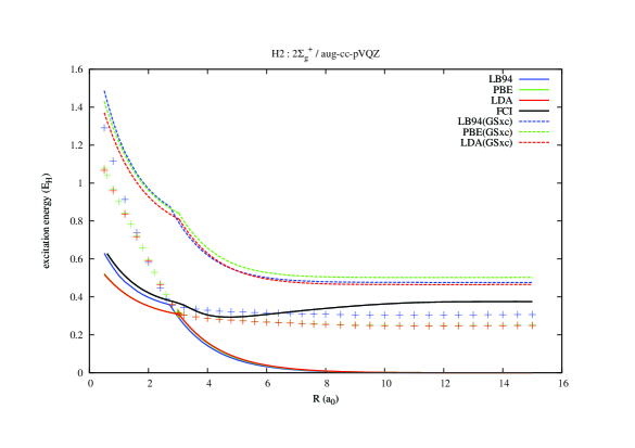
Figure 3: First ${}^{1}\Sigma_{g}^{+}$ excitation energy in H₂ along the bond-breaking coordinate obtained within the GSxc approximation with local and semi-local functionals (dashed colored lines). Comparison is made with FCI (solid black line) and with the KS excitation energy without the GSxc correction (solid colored lines). Crossings of singly- and doubly-excited KS states are shown for each functional with colored ”+” points. See text for further details.

5 Perspective: range-dependent GACE

Pastorczak et al. [21] recently formulated a multi-determinant extension of GOK-DFT that relies on the separation of the two-electron repulsion into long-range (lr) and short-range (sr) parts

$$\frac{1}{r_{12}}=w^{\rm lr,\mu}_{\rm ee}(r_{12})+w^{\rm sr,\mu}_{\rm ee}(r_{12}),$$ (136)

where $\mu$ is a parameter that controls the range separation with $w^{\rm lr,\mu}_{\rm ee}(r_{12})=1/r_{12}$ in the $\mu\rightarrow+\infty$ limit and $w^{\rm lr,\mu}_{\rm ee}(r_{12})=0$ for $\mu=0$. By analogy with ground-state multi-determinant range-separated DFT [54], they decomposed the universal GOK functional as follows

$$F^{w}[n] = F^{{\rm lr,\mu},w}[n]+{E}^{{\rm sr,\mu},w}_{\rm Hxc}[n],$$ (137)

where the universal long-range GOK functional is defined as

$$F^{{\rm lr,\mu},w}[n] = \underset{\{\Psi_{1},\Psi_{2}\}^{w}\rightarrow n}{\rm min}\Big{\{}(1-w)\,\langle\Psi_{1}|\hat{T}+\hat{W}^{\rm lr,\mu}_{\rm ee}|\Psi_{1}\rangle+w\,\langle\Psi_{2}|\hat{T}+\hat{W}^{\rm lr,\mu}_{\rm ee}|\Psi_{2}\rangle\Big{\}}$$ (138)

$$= (1-w)\,\langle\Psi^{\mu,w}_{1}|\hat{T}+\hat{W}^{\rm lr,\mu}_{\rm ee}|\Psi^{\mu,w}_{1}\rangle+w\,\langle\Psi^{\mu,w}_{2}|\hat{T}+\hat{W}^{\rm lr,\mu}_{\rm ee}|\Psi^{\mu,w}_{2}\rangle,$$

and ${E}^{{\rm sr,\mu},w}_{\rm Hxc}[n]$ is the $\mu$-dependent complementary short-range Hxc density functional for the ensemble. According to the GOK variational principle in Eq. (5), the exact ensemble energy can then be written as follows

$$E^{w} = (1-w)\,\langle\tilde{\Psi}^{\mu,w}_{1}|\hat{T}+\hat{W}^{\rm lr,\mu}_{\rm ee}|\tilde{\Psi}^{\mu,w}_{1}\rangle+w\,\langle\tilde{\Psi}^{\mu,w}_{2}|\hat{T}+\hat{W}^{\rm lr,\mu}_{\rm ee}|\tilde{\Psi}^{\mu,w}_{2}\rangle$$ (139)

$$+{E}^{{\rm sr,\mu},w}_{\rm Hxc}[n^{w}]+\int{\rm d}{\bf r}\,v_{\rm ne}({\bf r})\,n^{w}({\bf r}),$$

where the auxiliary long-range-interacting wave functions $\tilde{\Psi}^{\mu,w}_{i}\;(i=1,2)$ that reproduce the exact ensemble density $n^{w}$ fulfill the following self-consistent equations:

$$\Big{(}\hat{T}+\hat{W}^{\rm lr,\mu}_{\rm ee}+\hat{V}_{\rm ne}+\hat{{V}}^{{\rm sr,\mu},w}_{\rm Hxc}[n^{w}]\Big{)}|\tilde{\Psi}^{\mu,w}_{i}\rangle=\tilde{\mathcal{E}}^{\mu,w}_{i}|\tilde{\Psi}^{\mu,w}_{i}\rangle,\hskip 11.38092pti=1,2,$$

$${\displaystyle\hat{{V}}^{{\rm sr,\mu},w}_{\rm Hxc}[n]=\int{\rm d}{\mathbf{r}}\,\frac{\delta{E}^{{\rm sr,\mu},w}_{\rm Hxc}}{\delta n({\bf r})}[n]\,\hat{n}({\bf r}).}$$ (140)

While regular GOK-DFT and wavefunction theory approaches are recovered in the $\mu=0$ and $\mu\rightarrow+\infty$ limits, respectively, an exact state-average multi-determinant DFT is obtained for $0<\mu<+\infty$.

For convenience, Pastorczak et al. [21] substituted the ground-state short-range Hxc functional ${E}^{{\rm sr,\mu},0}_{\rm Hxc}[n]={E}^{{\rm sr,\mu}}_{\rm Hxc}[n]$ for the ensemble one in their practical calculations. This is a crude approximation which obviously can have an impact on the accuracy of the computed excitation energy, especially if small $\mu$ values are used [55, 56], since the range-separated approach is then closer to GOK-DFT than wavefunction theory. Better approximations might be developed from a range-dependent GACE. For that purpose we introduce the auxiliary equations

$$\Big{(}\hat{T}+\hat{W}^{\rm lr,\nu}_{\rm ee}+\hat{V}^{\nu,\xi}\Big{)}|\Psi^{\nu,\xi}_{i}\rangle=\mathcal{E}_{i}^{\nu,\xi}|\Psi^{\nu,\xi}_{i}\rangle,\hskip 5.69046pti=1,2,$$ (141)

where the local potential $\hat{V}^{\nu,\xi}=\int{\rm d}{\bf r}\,v^{\nu,\xi}({\bf r})\,\hat{n}({\bf r})$ ensures that the density constraint

$$n({\bf r}) = (1-\xi)\,n_{\Psi_{1}^{\nu,\xi}}({\bf r})+\xi\,n_{\Psi_{2}^{\nu,\xi}}({\bf r}),\hskip 11.38092pt0\leq\nu<+\infty,\hskip 11.38092pt0\leq\xi\leq w,$$ (142)

is fulfilled. By integration of the universal long-range GOK functional over the interval $[\mu,+\infty[$ we obtain from Eqs. (137), (138), (141) and (142),

$$\displaystyle E^{{\rm sr,\mu},w}_{\rm Hxc}[n] = \int^{+\infty}_{\mu}{\rm d}\nu\,\frac{{\rm d}}{{\rm d}\nu}F^{{\rm lr},\nu,w}[n]$$ (143)

$$= (1-w)\,\int^{+\infty}_{\mu}{\rm d}\nu\,\frac{{\rm d}\mathcal{E}_{1}^{\nu,w}}{{\rm d}\nu}+w\,\int^{+\infty}_{\mu}{\rm d}\nu\,\frac{{\rm d}\mathcal{E}_{2}^{\nu,w}}{{\rm d}\nu}$$

$$-\int^{+\infty}_{\mu}{\rm d}\nu\int{\rm d}\mathbf{r}\,\frac{\partial v^{\nu,w}({\bf r})}{\partial\nu}\,n({\bf r}),$$

which leads, according to the Hellmann–Feynman theorem, to the final expression

$$\displaystyle E^{{\rm sr,\mu},w}_{\rm Hxc}[n] = (1-w)\int^{+\infty}_{\mu}{\rm d}\nu\,\langle\Psi_{1}^{\nu,w}|\frac{\partial\hat{W}^{\rm lr,\nu}_{\rm ee}}{\partial\nu}|\Psi_{1}^{\nu,w}\rangle$$ (144)

$$+w\int^{+\infty}_{\mu}{\rm d}\nu\,\langle\Psi_{2}^{\nu,w}|\frac{\partial\hat{W}^{\rm lr,\nu}_{\rm ee}}{\partial\nu}|\Psi_{2}^{\nu,w}\rangle.$$

By analogy with GOK-DFT, we use a weight-independent definition for the ensemble short-range Hartree density-functional energy,

$$E^{{\rm sr},\mu,w}_{\rm H}[n]=E^{{\rm sr},\mu}_{\rm H}[n]=\frac{1}{2}\int\int{\rm d}{\mathbf{r}}{\rm d}{\mathbf{r^{\prime}}}n(\mathbf{r})n(\mathbf{r^{\prime}})w^{\rm sr,\mu}_{\rm ee}\left(|{\bf r}-{\bf r^{\prime}}|\right),$$ (145)

and thus define the short-range exchange–correlation energy for the ensemble as

$$E^{{\rm sr,\mu},w}_{\rm xc}[n]=E^{{\rm sr,\mu},w}_{\rm Hxc}[n]-E^{{\rm sr},\mu}_{\rm H}[n].$$ (146)

Like in the linear GACE that was introduced in Sec. 2.3, the exact deviation of the ensemble short-range exchange–correlation energy from the ground-state one can be derived by integration over the ensemble weight:

$${E}^{{\rm sr},\mu,w}_{\rm xc}[n] = {E}^{{\rm sr},\mu}_{\rm xc}[n]+\int_{0}^{w}{\rm d}\xi\,\Delta^{{\rm sr},\mu,\xi}_{\rm xc}[n],$$ (147)

where

$$\Delta^{{\rm sr},\mu,\xi}_{\rm xc}[n] = \frac{{\rm d}E^{{\rm sr,\mu},\xi}_{\rm Hxc}[n]}{{\rm d}\xi}$$ (148)

$$= \int^{+\infty}_{\mu}{\rm d}\nu\,\frac{{\rm d}^{2}F^{{\rm lr,\nu},\xi}[n]}{{\rm d}\nu{\rm d}\xi},$$

will be referred to as the short-range exchange–correlation DD since it reduces to the standard exchange–correlation DD when $\mu=0$. By analogy with the linear GACE (see Appendix 7), the derivative of the long-range GOK functional with respect to the ensemble weight equals

$$\displaystyle\frac{{\rm d}F^{{\rm lr,\nu},\xi}[n]}{{\rm d}\xi} = \mathcal{E}^{\nu,\xi}_{2}-\mathcal{E}^{\nu,\xi}_{1},$$ (149)

which leads to

$$\displaystyle\Delta^{{\rm sr},\mu,\xi}_{\rm xc}[n] = \Big{(}\mathcal{E}^{+\infty,\xi}_{2}-\mathcal{E}^{+\infty,\xi}_{1}\Big{)}-\Big{(}\mathcal{E}^{\mu,\xi}_{2}-\mathcal{E}^{\mu,\xi}_{1}\Big{)}.$$ (150)

In the particular case where $\xi=w$ and $n$ equals the exact ensemble density $n^{w}$, the first term on the right-hand side of Eq. (150) becomes the excitation energy $E_{2}-E_{1}$ of the true physical system while the second term reduces to the excitation energy $\tilde{\mathcal{E}}^{\mu,w}_{2}-\tilde{\mathcal{E}}^{\mu,w}_{1}$ of the long-range-interacting system whose ensemble density equals $n^{w}$ (see Eq. (5)), leading thus to the exact expression

$$\displaystyle E_{2}-E_{1} = \tilde{\mathcal{E}}^{\mu,w}_{2}-\tilde{\mathcal{E}}^{\mu,w}_{1}+\Delta^{{\rm sr},\mu,w}_{\rm xc}[n^{w}].$$ (151)

As readily seen from Eqs. (148) and (151), neglecting the weight dependence of the ensemble short-range exchange–correlation functional is equivalent to approximating the excitation energy with the long-range interacting one. In order to investigate the variation in $w$ and $\mu$ of the short-range exchange–correlation DD contribution, a simple procedure would consist in neglecting the weight dependence in the ensemble short-range exchange–correlation density-functional potential as Pastorczak et al. [21] did in their range-separated ensemble calculations, and computing the excitation energy difference $(E_{2}-E_{1})-(\tilde{\mathcal{E}}^{\mu,w}_{2}-\tilde{\mathcal{E}}^{\mu,w}_{1})$ at the CI level for various systems. The derivation of exact Taylor expansions in $w$ and $\mu$ for the short-range exchange–correlation DD, in the light of Sec. 2.3 and Ref. [54], would also be of interest for the development of approximate short-range ensemble functionals. Work is currently in progress in these directions.

6 Conclusions

A generalized adiabatic connection for ensembles (GACE) has been presented in this work. In contrast to the adiabatic connection (AC) proposed initially by Nagy [35], both ensemble weights and interaction strength vary along the GACE while the ensemble density is held fixed. For clarity the theory has been presented for non-degenerate two-state ensembles but the GACE can in principle be constructed for any ensemble consisting of an arbitrary number of non-degenerate states and complete sets of degenerate states [20]. Within such a formalism an exact expression for the deviation of the ensemble exchange–correlation density-functional energy from the conventional ground-state one has been derived. Levy’s stringent constraint of Ref. [6] has been recovered when expanding the ensemble exchange–correlation functional through second order in the ensemble weight. In addition, an explicit expression for the exchange–correlation derivative discontinuity contribution to this condition has been obtained within the GACE. In the light of the recent work of Teale et al. [31, 32, 33] on the accurate computation of ground-state ACs, we briefly explained how the GACE could be constructed by using a Legendre–Fenchel transform for ensembles. As an illustration, the GACE has been derived analytically for the H₂ model system in a minimal basis, providing thus a simple density-functional approximation for two-state ensembles. This approximation has been tested with a large basis on the calculation of the first ${}^{1}\Sigma^{+}_{g}$ excitation energy in H₂ upon bond stretching. Encouraging results were obtained at large distance (the double excitation could be described) but better ensemble exchange–correlation functionals are needed for describing the excitation at all bond distances, especially in order to reproduce the avoided crossing at $R=3$ a.u. A more accurate description of the GACE would be useful for developing such functionals. Following Pastorczak et al. [21], we finally discussed as a perspective the development of a state-average multi-determinant DFT approach based on a range-dependent GACE. Exact expressions for the complementary short-range ensemble exchange–correlation density-functional energy have been derived and guidelines for the development of density-functional approximations have been provided. Work is currently in progress in this direction. We hope that the paper will stimulate further developments in ensemble DFT.

7 Derivative of the partially-interacting GOK functional with respect to the ensemble weight

When rewriting, according to Eqs. (17) and (18), the partially-interacting GOK functional as

$$F^{\lambda,\xi}[n] = (1-\xi)\,\mathcal{E}_{1}^{\lambda,\xi}+\xi\,\mathcal{E}_{2}^{\lambda,\xi}-\int{\rm d}{\bf r}\,v^{\lambda,\xi}({\bf r})\,{n}({\bf r})$$ (152)

we obtain

$$\displaystyle\frac{{\rm d}F^{\lambda,\xi}[n]}{{\rm d}\xi} = \mathcal{E}^{\lambda,\xi}_{2}-\mathcal{E}^{\lambda,\xi}_{1}+(1-\xi)\,\frac{{\rm d}\mathcal{E}_{1}^{\lambda,\xi}}{{\rm d}\xi}+\xi\,\frac{{\rm d}\mathcal{E}_{2}^{\lambda,\xi}}{{\rm d}\xi}$$ (153)

$$-\int{\rm d}{\bf r}\,\frac{\partial v^{\lambda,\xi}({\bf r})}{\partial\xi}\,{n}({\bf r}),$$

which, according to the Hellmann–Feynman theorem in Eq. (31) and the density constraint in Eq. (18), leads to Eq. (23).

8 Exact local potential for the non-interacting ensemble

According to the GOK variational principle the density $n$ for which the GACE is constructed minimizes the density-functional ensemble energy

$$\mathcal{E}^{\xi}[\rho]=T^{\xi}_{\rm s}[\rho]+{E}^{\xi}_{\rm Hxc}[\rho]+\int{\rm d}{\bf r}\,\bigg{(}v^{1,\xi}({\bf r})+C\bigg{)}\,\rho({\bf r})$$ (154)

where $C$ is an arbitrary constant. The minimum equals $(1-\xi)\mathcal{E}_{1}^{1,\xi}+\xi\,\mathcal{E}_{2}^{1,\xi}+CN$ where $N$ denotes the number of electrons (which is fixed in this work). Consequently

$$\left.\frac{\delta}{\delta\rho({\bf r})}\Bigg{[}\mathcal{E}^{\xi}[\rho]+\mu^{\xi}\Bigg{(}\int{\rm d}{\mathbf{r}\,\rho(\mathbf{r})}-N\Bigg{)}\Bigg{]}\right|_{\rho=n}$$

$$=\frac{\delta T^{\xi}_{\rm s}}{\delta\rho({\bf r})}[n]+\frac{\delta{E}^{\xi}_{\rm Hxc}}{\delta\rho({\bf r})}[n]+v^{1,\xi}({\bf r})+C+\mu^{\xi}$$

$$=0,$$ (155)

where the Lagrange multiplier $\mu^{\xi}$ is the chemical potential. When choosing $C=-\mu^{\xi}$, we finally obtain Eq. (34) since

$$\frac{\delta T^{\xi}_{\rm s}}{\delta\rho({\bf r})}[n]=-v^{0,\xi}({\bf r}).$$ (156)

9 Maximum of the ground-state Legendre–Fenchel transform for H₂ in a minimal basis

According to Eq. (87) the first-order derivative of the auxiliary ground-state energy can be expressed as

$$\frac{{\rm d}\mathcal{E}^{\lambda}_{1}(\upsilon)}{{\rm d}\upsilon}=\frac{\lambda}{2}\left(1-\frac{\delta+\upsilon}{\sqrt{\big{(}\delta+\upsilon\big{)}^{2}+4K^{2}}}\right),$$ (157)

where $\delta=E_{g}-E_{u}$. Using

$$\left[\sqrt{\big{(}\delta+\upsilon\big{)}^{2}+4K^{2}}-(\delta+\upsilon)\right]\left[\sqrt{\big{(}\delta+\upsilon\big{)}^{2}+4K^{2}}+(\delta+\upsilon)\right]=4K^{2},$$ (158)

Eq. (157) becomes

$$\frac{{\rm d}\mathcal{E}^{\lambda}_{1}(\upsilon)}{{\rm d}\upsilon} = \frac{2\lambda K^{2}}{\sqrt{\big{(}\delta+\upsilon\big{)}^{2}+4K^{2}}\left[\sqrt{\big{(}\delta+\upsilon\big{)}^{2}+4K^{2}}+(\delta+\upsilon)\right]}$$ (159)

$$= \frac{2\lambda K^{2}}{(\delta+\upsilon)\left[(\delta+\upsilon)+\sqrt{\big{(}\delta+\upsilon\big{)}^{2}+4K^{2}}\right]+4K^{2}}.$$

Since, according to Eqs. (67) and (69),

$$1+C^{2}_{u} = 1+\frac{1}{4K^{2}}\left(\delta+\sqrt{\delta^{2}+4K^{2}}\right)^{2}$$ (160)

$$= \frac{4K^{2}+\delta\left(\delta+\sqrt{\delta^{2}+4K^{2}}\right)}{2K^{2}},$$

we conclude that Eq. (89) is equivalent to

$$f(\upsilon)=f(0),$$ (161)

where the function $f$ is defined as

$$f(\upsilon)=(\delta+\upsilon)\left[(\delta+\upsilon)+\sqrt{\big{(}\delta+\upsilon\big{)}^{2}+4K^{2}}\right].$$ (162)

Finally, since

$$\frac{{\rm d}f}{{\rm d}\upsilon}=\frac{\left[(\delta+\upsilon)+\sqrt{\big{(}\delta+\upsilon\big{)}^{2}+4K^{2}}\right]^{2}}{\sqrt{\big{(}\delta+\upsilon\big{)}^{2}+4K^{2}}}>0,$$ (163)

$f$ is monotonically increasing with $\upsilon$ which leads to Eq. (90).

References

- [1] M. Casida and M. Huix-Rotllant, Annu. Rev. Phys. Chem. 63, 287 (2012).
- [2] A.K. Theophilou, J. Phys. C (Solid State Phys.) 12, 5419 (1979).
- [3] J. Stoddart and K. Davis, Solid State Commun. 42, 147 (1982).
- [4] W. Kohn, Phys. Rev. A 34, 737 (1986).
- [5] E.K.U. Gross, L.N. Oliveira and W. Kohn, Phys. Rev. A 37, 2809 (1988).
- [6] M. Levy, Phys. Rev. A 52, R4313 (1995).
- [7] A. Görling, Phys. Rev. A 54, 3912 (1996).
- [8] A. Görling, Phys. Rev. A 59, 3359 (1999).
- [9] M. Levy and A. Nagy, Phys. Rev. Lett. 83, 4361 (1999).
- [10] M. Levy and A. Nagy, Phys. Rev. A 59, 1687 (1999).
- [11] N.I. Gidopoulos, P.G. Papaconstantinou and E.K.U. Gross, Phys. Rev. Lett. 88, 033003 (2002).
- [12] V. Sahni and X.Y. Pan, Phys. Rev. Lett. 90, 123001 (2003).
- [13] R. Gaudoin and K. Burke, Phys. Rev. Lett. 93, 173001 (2004).
- [14] R. Gaudoin and K. Burke, Phys. Rev. Lett. 94, 029901 (2005).
- [15] A. Kazaryan, J. Heuver and M. Filatov, J. Phys. Chem. A 112, 12980 (2008).
- [16] P.W. Ayers and M. Levy, Phys. Rev. A 80, 012508 (2009).
- [17] T. Ziegler, M. Seth, M. Krykunov, J. Autschbach and F. Wang, J. Chem. Phys. 130, 154102 (2009).
- [18] P.W. Ayers, M. Levy and A. Nagy, Phys. Rev. A 85, 042518 (2012).
- [19] M. Krykunov and T. Ziegler, J. Chem. Th. Comp. 9, 2761 (2013).
- [20] E.K.U. Gross, L.N. Oliveira and W. Kohn, Phys. Rev. A 37, 2805 (1988).
- [21] E. Pastorczak, N.I. Gidopoulos and K. Pernal, Phys. Rev. A 87, 062501 (2013).
- [22] L.N. Oliveira, E.K.U. Gross and W. Kohn, Phys. Rev. A 37, 2821 (1988).
- [23] I. Andrejkovics and A. Nagy, Chem. Phys. Lett. 296, 489 (1998).
- [24] G. Paragi, I. Gyémánt and V.V. Doren, J. Mol. Struct. (Theochem) 571, 153 (2001).
- [25] G. Paragi, I. Gyémánt and V.V. Doren, Chem. Phys. Lett. 324, 440 (2000).
- [26] D.C. Langreth and J.P. Perdew, Solid State Commun. 17, 1425 (1975).
- [27] O. Gunnarsson and B.I. Lundqvist, Phys. Rev. B 13, 4274 (1976).
- [28] O. Gunnarsson and B.I. Lundqvist, Phys. Rev. B 15, 6006 (1977).
- [29] D.C. Langreth and J.P. Perdew, Phys. Rev. B 15, 2884 (1977).
- [30] A. Savin, F. Colonna and R. Pollet, Int. J. Quantum Chem. 93, 166 (2003).
- [31] A.M. Teale, S. Coriani and T. Helgaker, J. Chem. Phys. 130, 104111 (2009).
- [32] A.M. Teale, S. Coriani and T. Helgaker, J. Chem. Phys. 132, 164115 (2010).
- [33] A.M. Teale, S. Coriani and T. Helgaker, J. Chem. Phys. 133, 164112 (2010).
- [34] Y. Cornaton, O. Franck, A.M. Teale and E. Fromager, Mol. Phys. 111, 1275 (2013).
- [35] A. Nagy, Int. J. Quantum Chem. 56, 225 (1995).
- [36] A. Nagy, J. Phys. B: At. Mol. Opt. Phys. 29, 389 (1996).
- [37] P. Hohenberg and W. Kohn, Phys. Rev. 136, B864 (1964).
- [38] H. Eschrig, The Fundamentals of Density Functional Theory, 2nd ed. (Eagle, Leipzig, 2003 ; Edition am Gutenbergplatz), Edition am Gutenbergplatz.
- [39] W. Kutzelnigg, J. Mol. Structure: THEOCHEM 768, 163 (2006).
- [40] R. van Leeuwen, Adv. Quantum Chem. 43, 25 (2003).
- [41] E.H. Lieb, Int. J. Quantum Chem. 24, 243 (1983).
- [42] S.M. Valone, J. Chem. Phys. 73, 4653 (1980).
- [43] M.J.S. Dewar and J. Kelemen, J. Chem. Educ. 48, 494 (1971).
- [44] K. Sharkas, A. Savin, H.J. Aa. Jensen and J. Toulouse, J. Chem. Phys. 137, 044104 (2012).
- [45] J.E. Harriman, Phys. Rev. A 27, 632 (1983).
- [46] D.R. Rohr and A. Savin, J. Mol. Struct.: THEOCHEM 943, 90 (2010).
- [47] P. Ayers, Theor. Chem. Acc. 118, 371 (2007).
- [48] S.H. Vosko, L. Wilk and M. Nusair, Can. J. Phys. 58, 1200 (1980).
- [49] J.P. Perdew, K. Burke and M. Ernzerhof, Phys. Rev. Lett. 77, 3865 (1996).
- [50] R. van Leeuwen and E.J. Baerends, Phys. Rev. A 49, 2421 (1994).
- [51] T.H. Dunning, J. Comp. Phys. 90, 1007 (1989).
- [52] DALTON, a molecular electronic structure program, Release Dalton2011 (2011), see http://daltonprogram.org/ .
- [53] K.J.H. Giesbertz, O.V. Gritsenko and E.J. Baerends, J. Chem. Phys. 136 (9), 094104 (2012).
- [54] J. Toulouse, F. Colonna and A. Savin, Phys. Rev. A 70, 062505 (2004).
- [55] E. Fromager, J. Toulouse and H.J. Aa. Jensen, J. Chem. Phys. 126, 074111 (2007).
- [56] E. Fromager, S. Knecht and H.J. Aa. Jensen, J. Chem. Phys. 138, 084101 (2013).