Vibrational mode multiplexing of ultracold atoms

Abstract

Sending multiple messages on qubits encoded in different vibrational modes of cold atoms or ions along a transmission waveguide requires to merge first and then separate the modes at input and output ends. Similarly, different qubits can be stored in the modes of a trap and be separated later. We design the fast splitting of a harmonic trap into an asymmetric double well so that the initial ground vibrational state becomes the ground state of one of two final wells, and the initial first excited state becomes the ground state of the other well. This might be done adiabatically by slowly deforming the trap. We speed up the process by inverse engineering a double-function trap using dynamical invariants. The separation (demultiplexing) followed by an inversion of the asymmetric bias and then by the reverse process (multiplexing) provides a population inversion protocol based solely on trap reshaping.

Introduction.– One of the main goals of atomic physics is to achieve an exhaustive control of atomic states and dynamics advances . The ultra-cold domain is particularly suitable for this aim as it provides a rich scenario of quantum states and phenomena. Atom optics and atomtronics atom intend to manipulate cold atoms in circuits and devices for applications in metrology, quantum information, or fundamental science. These devices are frequently inspired by electronics (e.g. the atom diode ad1 ; at2 , the transistor atom , atom chips chips ), or optics (e.g. beam splitters bs , or multiplexing optics1 ; optics2 ).

Figure 1: Population inversion using trap deformations in three steps: demultiplexing, bias inversion, and multiplexing.

In this paper we shall focus on a cold-atom realization of multiplexing, a basic process in modern telecommunications. Multiplexing is the transmission of different messages via a single physical medium. A multiplexer combines signals from several emitters into a single medium whereas a demultiplexer performs the reverse operation. The concept of multiplexing is relevant for quantum information processing (for its use in quantum repeaters see multip1 ; multip2 , or for trapped ions multip3 ). We envision here optical or magnetic waveguides for atoms holding several transverse orthogonal modes ion ; wg1 ; wg2 ; wg3 . If the qubit is encoded in the internal state of the atom, several qubits may be carried out simultaneously by different modes. To develop such a quantum-information architecture, fast multiplexers/demultiplexers that could join the modes from different waveguides into one guide, or separate them, are needed. We shall discuss trap designs for demultiplexing since the multiplexer would simply operate in reverse. For a proof-of-principle we propose the simplified setting of a single initial harmonic trap for non-interacting cold atoms whose first two eigenstates will be separated, as in the first step of Fig. 1, into two different wells. In a complete demultiplexing process the final wells should be independent, with negligible tunneling. The challenge is to design the splitting (a) without final excitation of higher vibrational levels, (b) in a short time, and (c) with a realizable trap potential. Condition (a) may be achieved by an adiabatic asymmetric splitting Gea ; split in which, for moderate bias compared to the vibrational quanta, the initial ground state becomes the ground state of the well with the lowest energy, and the excited state becomes the ground state of the other well. This adiabatic approach generally fails to satisfy the condition (b) which we shall implement applying “shortcuts to adiabaticity” Chen ; ChenPRA ; review ; Bowler . As for (c), we shall make use of a simple two-level model for the shortcut design, and then map it to a realistic potential recently implemented to realize an atomic Josephson junction Oberthaler . Finally, several applications, such as separation of multiple modes, population inversion, or controlled excitation, will be discussed.

Slow adiabatic and fast adiabatic processes.– Suppose that a harmonic potential evolves adiabatically into two well-separated and asymmetric wells as in the first step of Fig. 1. To accelerate the dynamics we shall use a moving two-level approximation based on a (yet-unspecified) process where a symmetrical potential evolves from an initial harmonic trap to a final double well. Then, we construct a time-dependent orthogonal bare basis $|L(t)\rangle=\left(\scriptsize{\begin{array}[]{rccl}0\\ 1\end{array}}\right)$, $|R(t)\rangle=\left(\scriptsize{\begin{array}[]{rccl}1\\ 0\end{array}}\right)$ of left and right states, obtained by a linear combination of the instantaneous ground and first excited states. An approximate two-mode Hamiltonian model for a generally asymmetrical process is written in this basis as

$$H_{2\times 2}(t)=\frac{\hbar}{2}\left(\begin{array}[]{cc}\lambda(t)&-\delta(t)\\ -\delta(t)&-\lambda(t)\end{array}\right),$$ (1)

where, for the double well configuration, $\delta(t)$ is the tunneling rate, and $\hbar\lambda(t)$ the relative gap, or bias, between the two wells. For the initial harmonic potential at $t=0$, $\lambda(0)=0$ and $\delta(0)=\omega_{0}$. The instantaneous eigenvalues are $E^{\pm}_{\lambda}(t)=\pm\frac{\hbar}{2}\sqrt{\lambda^{2}(t)+\delta^{2}(t)}$, and the normalized eigenstates

$$|\psi^{+}_{\lambda}(t)\rangle = \sin{\left(\frac{\alpha}{2}\right)}|L(t)\rangle-\cos{\left(\frac{\alpha}{2}\right)}|R(t)\rangle,$$ (2)

$$|\psi^{-}_{\lambda}(t)\rangle = \cos{\left(\frac{\alpha}{2}\right)}|L(t)\rangle+\sin{\left(\frac{\alpha}{2}\right)}|R(t)\rangle,$$

where the mixing angle $\alpha=\alpha(t)$ is given by $\tan\alpha=\delta(t)/\lambda(t)$. The boundary conditions on $\lambda(t)$ and $\delta(t)$ are

$$\delta(0)=\omega_{0},\,\,\lambda(0)=0,\,\,\delta(t_{f})=0,\,\,\lambda(t_{f})=\lambda_{f},$$ (3)

which correspond, at time $t=0$, to a harmonic well, and at time $t_{f}$ to two independent wells with asymmetry bias $\hbar\lambda_{f}$.

To design a fast, but still adiabatic process, we shall first assume the simplifying conditions: $\lambda(t)=\lambda$ constant and $\lambda/\delta(0)\ll 1$. Thus $\alpha(0)\approx\pi/2$ and the initial eigenstates essentially coincide with the ground and first excited states of the harmonic oscillator. For a constant $\lambda$ the adiabaticity condition reads split $\left|\frac{\lambda\dot{\delta}(t)}{2(\lambda^{2}+\delta(t)^{2})^{3/2}}\right|\ll 1$. Imposing a constant value $c$ for the adiabaticity parameter and using the boundary conditions for $\delta$ in Eq. (3), we fix the integration constant and the value of $c$, $c=\frac{\omega_{0}}{2\lambda\sqrt{\omega_{0}^{2}+\lambda^{2}}\,t_{f}}$. The “fast adiabatic” solution of the differential equation for $\delta(t)$ takes finally the form $\delta_{fa}(t)=\frac{\omega_{0}\lambda(t_{f}-t)}{\sqrt{{\lambda^{2}t_{f}^{2}+\omega_{0}^{2}t(2t_{f}-t)}}}$. However, to keep adiabaticity, $c\ll 1$ should hold, so this protocol is limited by $t_{f}\gg\frac{1}{2\lambda}\gg\frac{1}{\omega_{0}}$. We shall now work out an alternative, faster protocol based on invariants in which the boundary conditions on $\lambda(t)$ and $\delta(t)$ will be satisfied exactly.

Invariant-based inverse engineering.– For the Hamiltonian in Eq. (1) there is a dynamical invariant $I(t)$ of the form ChenPRA

$$I(t)=\frac{\hbar}{2}\Omega_{0}\left(\begin{array}[]{cc}\cos\theta(t)&\sin\theta(t)e^{i\varphi(t)}\\ \sin\theta(t)e^{-i\varphi(t)}&-\cos\theta(t)\end{array}\right),$$ (4)

where $\varphi(t)$ and $\theta(t)$ are auxiliary (azymuthal and polar) angles, and $\Omega_{0}$ is an arbitrary constant with units of frequency. The eigenvectors of $I(t)$ multiplied by Lewis-Riesenfeld phase factors provide two orthogonal solutions of the time-dependent Schrödinger equation ChenPRA . To inverse engineer the Hamiltonian we design the invariant first, and then deduce the Hamiltonian from it. The boundary conditions $[H_{2\times 2}(t),I(t)]=0$ will be applied at the interval ends $t_{b}=0,\,t_{f}$, so that the eigenvectors of $I(t_{b})$ and $H_{2\times 2}(t_{b})$ coincide. The role of the invariant is therefore to drive the initial eigenstates of $H_{2\times 2}(0)$ to the eigenstates of $H_{2\times 2}(t_{f})$. In our application this implies a unitary mapping from the first two eigenstates of the harmonic oscillator to the ground states of the left and right final wells.

From the invariance property $i\hbar\frac{\partial I(t)}{\partial t}-[H_{2\times 2}(t),I(t)]=0$, it follows that

$$\delta(t) = -\dot{\theta}(t)/\sin{\varphi(t)},$$ (5)

$$\lambda(t) = -\delta(t)\cot{\theta(t)}\cos{\varphi(t)}-\dot{\varphi}(t).$$

The commutativity of $I(t)$ and $H_{2\times 2}(t)$ at boundary times $t_{b}=0,t_{f}$ imposes the conditions

$$\begin{array}[]{ll}\lambda(t_{b})\sin[\theta(t_{b})]e^{i\varphi(t_{b})}+\delta(t_{b})\cos[\theta(t_{b})]=0,\\ \lambda(t_{b})\sin[\theta(t_{b})]e^{-i\varphi(t_{b})}+\delta(t_{b})\cos[\theta(t_{b})]=0,\\ \delta(t_{b})\sin[\theta(t_{b})]\sin[\varphi(t_{b})]=0,\end{array}$$ (6)

Taking into account Eqs. (3) we get from Eq. (6)

$$\theta(0)=\pi/2,\;\;\varphi(0)=\pi,\;\;\theta(t_{f})=\pi,\;\;\dot{\theta}(t_{f})=0.$$ (7)

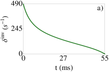
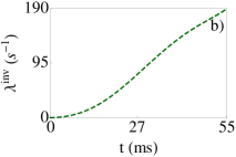
Figure 2: (Color online) (a) $\delta^{\rm{inv}}(t)$ and (b) $\lambda^{\rm{inv}}(t)$. $\delta(0)=2\pi\times 78$ Hz, $\lambda_{f}=190$ s^-1, $\dot{\lambda}(0)=190$ s^-2, and $t_{f}=55$ ms.

These conditions lead to indeterminacies in Eq. (5). To resolve them we apply L’Hôpital’s rule repeatedly and find additional boundary conditions,

$$\dot{\theta}(0)\! \!=\! \ddot{\theta}(0)=\dot{\varphi}(0)=0,\,\,\dddot{\theta}(0)=-\omega_{0}\dot{\lambda}(0),$$ (8)

$$\ddot{\varphi}(0)\! \!=\! -\dot{\lambda}(0),\,\,\varphi(t_{f})=\pi/2,\;\;\dot{\varphi}(t_{f})=-\frac{\lambda_{f}}{3}.$$

with $\dot{\lambda}(0)\neq 0$. At intermediate times, we interpolate the angles assuming a polynomial ansatz, $\theta(t)=\sum_{j=0}^{5}a_{j}t^{j}$ and $\varphi(t)=\sum_{j=0}^{4}b_{j}t^{j}$, where the coefficients are found by solving the equations for the boundary conditions. Thus we obtain the Hamiltonian functions $\delta^{\rm{inv}}(t)$ and $\lambda^{\rm{inv}}(t)$ from Eq. (5). Figure 2 provides an example of parameter trajectories.

Mapping to coordinate space.– Our purpose now is to map the $2\times 2$ Hamiltonian into a realizable potential

$$V(x,t)=\frac{1}{2}m\omega^{2}x^{2}+V_{0}\cos^{2}\left[\frac{\pi(x-\Delta x)}{d_{l}}\right].$$ (9)

This form has been already implemented Oberthaler with optical dipole potentials, combining a harmonic confinement due to a crossed beam dipole trap with a periodic light shift potential provided by the interference pattern of two mutually coherent laser beams. The control parameters are in principle the frequency $\omega$, the displacement $\Delta x$ of the optical lattice relative to the center of the harmonic well, the amplitude $V_{0}$, and the lattice constant $d_{l}$, but in the following examples we fix $d_{l}$ and $\Delta x$; the other two parameters offer enough flexibility and are easier to control as time-dependent functions. To perform the mapping, we minimize numerically $F[V_{0}(t),\omega(t)]=[\delta^{\rm{id}}(t)-\delta(t)]^{2}+[\lambda^{\rm{id}}(t)-\lambda(t)]^{2}$, using the simplex method. The functions $\delta^{\rm{id}}(t)$ and $\lambda^{\rm{id}}(t)$ are designed according to the shortcuts discussed before, and $\delta(t)$ and $\lambda(t)$ are computed as $\delta(t)=-\frac{2}{\hbar}\langle L(t)|H|R(t)\rangle=-\frac{2}{\hbar}\langle R(t)|H|L(t)\rangle$, $\lambda(t)=\frac{2}{\hbar}\langle R(t)|H-\Lambda|R(t)\rangle=-\frac{2}{\hbar}\langle L(t)|H-\Lambda|L(t)\rangle$, where $H=H(V_{0}(t),\omega(t);\Delta x,d_{l})=-\frac{\hbar^{2}}{2m}\frac{\partial^{2}}{\partial x^{2}}+V$ is the full Hamiltonian in coordinate space with a kinetic energy term and the potential (9); $\Lambda(t)=[E_{\lambda}^{-}(t)+E_{\lambda}^{+}(t)]/2$ is a shift defined from the first two levels $E_{\mp}$ of $H$ to match the zero-energy point between the coordinate and the two-level system; finally, $|R(t){\rangle}=(|g(t){\rangle}+|e(t){\rangle})/2^{1/2}$ and $|L(t){\rangle}=(|g(t){\rangle}-|e(t){\rangle})/2^{1/2}$ form the base, where $|g(t){\rangle}$ is the ground state and $|e(t){\rangle}$ the first excited state of the symmetrical Hamiltonian $H_{0}(V_{0}(t),\omega(t);\Delta x=0,d_{l})$, defined as $H$ but with $\Delta x=0$, which we diagonalize numerically. In our calculations, $\delta(t)$ and $\lambda(t)$ become indistinguishable from their ideal counterparts. Figure 3 depicts $V_{0}(t)$ and $\omega(t)$ for the parameters of Fig. 2. We use ⁸⁷Rb atoms and a lattice spacing $d_{l}=5.18$ $\mu$m. The sharp final increase of $V_{0}(t)$ makes the two wells totally independent but, for most applications this strict condition may be relaxed to avoid intra-well excitations.

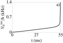
Figure 3: Lattice height $V_{0}$, and trap frequency $\omega/(2\pi)$ using invariant-based engineering and mapping. $\Delta x=200$ nm.

Figure 4 demonstrates perfect transfer for the ground (a) and the excited state (b) using the very same protocol in both cases, the one depicted in Figs. 2 and 3. (Thanks to the superposition principle, the same protocol would produce a perfect demultiplexing for any linear combination of the ground and excited states.) Initial and final states are represented, solving the Schrödinger equation with the potential (9). We stop the process $2$ ms before the nominal time $t_{f}$ as the fidelity reaches a stable maximum there and a further increase of $V_{0}$ is not required. We also include the results for the protocol in which $\omega$ is kept constant and $V_{0}(t)$ is a linear ramp (with the same durations as the shortcut protocols). For this linear protocol the final state includes a significant density in the “wrong” well. This simple linear-$V_{0}$ approach needs $t_{f}\gtrsim 0.7$ s to become adiabatic and produce the same fidelity, 0.9997, found for a shortcut protocol ten times faster, $t_{f}=0.07$ s, the rightmost point in Fig. 5 (a). Fig. 6 compares the populations in the instantaneous basis of the (full, coordinate-space) Hamiltonian for the shortcut and the linear protocols when the system starts in the ground state, corresponding to Fig. 4 (a). The shortcut protocol implies a transient exchange between ground and (first) excited levels but finally takes the system to the desired ground state. In contrast for the linear protocol the excitation is permanent leading to a poor final fidelity.

In the two-level model $t_{f}$ may be reduced arbitrarily, but in the coordinate space Hamiltonian levels 0-1 will only be “independent” as long as higher levels are not excited. These excitations are the limiting factor to shorten the times further with the current mapping scheme. Some guidance is provided by the Anandan-Aharonov relation $t_{f}>h/(4\overline{\Delta E})$, where $\overline{\Delta E}$ is the time average of the standard deviation AA .

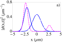
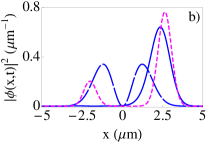
Figure 4: (Color online) (a): Ground state at $t=0$ (long-dashed, blue line); final state with the shortcut (solid, blue line, indistinguishable from the ground state of the final trap); final state with linear ramp for $V_{0}(t)$ and $\omega=2\pi\times 78$ Hz (short-dashed, magenta line). (b): Same as (a) for the first excited state. Parameters like in Fig. 3 at $t=53$ ms. The linear ramp for $V_{0}(t)$ ends in the same value used for the shortcut.

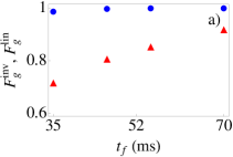
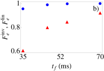
Figure 5: (Color online) Fidelities with respect to the final ground state starting at the ground state (a) and with respect to the final first excited state starting at the excited state (b) versus final time $t_{f}$, via shortcuts ($F_{g}^{inv}$ and $F_{e}^{inv}$, blue circles), or linear ramping of $V_{0}(t)$ ($F_{g}^{lin}$ and $F_{e}^{lin}$, red triangles). The fidelity is computed at 2 ms less than the nominal $t_{f}$. Other parameters as in Figs. 2, 3, and 4.

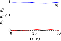
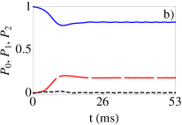
Figure 6: (Color online) Populations of the states for the shortcuts (a) and the linear ramp for $V_{0}(t)$ (b). Ground state ($P_{0}$, solid blue line); First excited state ($P_{1}$, long-dashed red line); Second excited state ($P_{2}$, short-dashed black line). Parameters as in Fig. 4 (a).

Discussion.– Vibrational multiplexing may be combined with internal-state multiplexing multip3 to provide a plethora of possible operations. Motivated by the prospective use of multiplexing/demultiplexing for quantum information processing, we have applied shortcuts-to-adiabaticity techniques to speed up the spatial separation of vibrational modes of a harmonic trap. A similar approach would separate $n$ modes into $n$ wells so as to deliver more information into different processing sites. The number of modes that could be separated will depend on the asymmetric bias in relation to other potential parameters: the bias among the extreme wells should not exceed the vibrational quanta in the final wells. The bias determines possible speeds too, as smaller biases generally imply longer times.

A previous work split dealt also with splitting operations and shortcuts to adiabaticity, but the objective was the opposite to our aim here. Since adiabatic following from a harmonic trap to an asymmetric double well collapses the ground state wave to one of the two wells, a “fast-forward” (FF) technique Masuda ; ourff was applied to avoid the collapse and achieve perfect, balanced splitting, as required, e.g., for matter-wave interferometry. The idea was that for a fast non-adiabatic shortcut the perturbative effect of the asymmetry becomes negligible. The stabilizing effect of interactions was also characterized within a mean-field treatment. In the present paper the objective is to send each mode of the initial harmonic trap as fast as possible to a different final well, so we needed a different methodology. Instead of FF, which demands an arbitrary control of the potential function in position and time, we have restricted the potential to a form with a few controllable parameters (in practice we have let only two of them evolve in time). Inverse engineering of the Hamiltonian is carried out for a two-level model using invariants of motion, and the resulting (analytical) Hamiltonian is then mapped to real space. The discrete Hamiltonian is useful as it provides a simple picture to understand and design the dynamics at will. In future work we shall increase the number of levels in the discrete model and test alternative potential functions. The method provides also a good basis to apply optimal control theory (OCT), which complements invariant-based engineering, see. e.g. Li , by selecting among the fidelity-one protocols according to other physical requisites. As for interactions and nonlinearities, they will generally spoil a clean multiplexing/demultiplexing processes, so we have only examined linear dynamics here.

An application of the demultiplexing schemes discussed in this work is the population inversion of the first two levels of the harmonic trap without making use of internal state excitations Salomon . This is useful to avoid decoherence effects induced by decay, or for species without an appropriate (isolated two-level) structure. The scheme is based on the three steps shown in Fig. 1. A mechanical excitation of the ground state level into the first excited state of a fixed anharmonic potential was implemented by shaking the trap along a trajectory calculated with an OCT algorithm ms_schmiedmayer . Our proposed approach relies instead on a smooth potential deformation. This type of inversion could be applied to interacting Bose-Einstein condensates as long as the initial states are pure ground or excited levels. The production of twin-atom beams from the excited state is an outstanding application twin .

Asymmetric double wells may also be used for other state-control operations such as preparing non-equilibrium Fock states through a ladder excitation process. The vibrational number may be increased by one at every step. Each excitation would start and finish with demultiplexing and multiplexing operations from the harmonic oscillator to the double well and viceversa, as described in the main text. Between them the two wells are independent and their height or width can be adjusted to produce the desired level ordering. For an even-to-odd vibrational number transition this requires an inversion of the bias, as in Fig. 1; transitions from odd to even levels are performed by deepening the left well until the initially occupied level on the right well surpasses one of the levels in the left well. The steps may be repeated until a given Fock state is reached. Operating in reverse mode, a given excited state could be taken down to the ground state, as in sideband cooling, just with trap deformations.

Open questions left for future work include optimizing the robustness of parameter trajectories versus noise and perturbations Andreas , or finding time bounds in terms of average energies, similar to the ones for harmonic trap expansions energy or transport transport . The present results may also be applied for optical waveguide design SCh , or to 2D systems as a way to generate vortices.

Acknowledgment.– This work was supported by the National Natural Science Foundation of China (Grant No. 61176118), the Grants No. 12QH1400800 IT472-10, BFI-2010-255, 13PJ1403000, FIS2012-36673-C03-01, and the program UFI 11/55. S. M.-G. acknowledges a fellowship by UPV/EHU.

References

- (1) C. Cohen-Tannoudji and D. Guéry-Odelin, Advances in atomic physics: an overview (World Scientific, Singapore, 2011).
- (2) B. T. Seaman, M. Krämer, D. Z. Anderson, and M. J. Holland, Phys. Rev. A 75, 023615 (2007).
- (3) A. Ruschhaupt and J. G. Muga, Phys. Rev. A 70, 061604(R) (2004).
- (4) M. G. Raizen, A. M. Dudarev, Qian Niu, and N. J. Fisch, Phys. Rev. Lett. 94, 053003 (2005).
- (5) Atom Chips, ed. by R. Reichel and V. Vuletic, Wiley-VCH, Weinheim 2011.
- (6) G. L. Gattobigio, A. Couvert, G. Reinaudi, B. Georgeot, and D. Guéry-Odelin, Phys. Rev. Lett. 109, 030403 (2012).
- (7) W. K. Burns and A. F. Milton, IEEE J. Quant. Elect. QE-11, 32 (1975).
- (8) N. Riesen and J. D. Love, Applied Opt. 51, 2778 (2012).
- (9) N. Sangouard, C. Simon, H. Riedmatten, and N. Gisin, Rev. Mod. Phys. 83, 33 (2011).
- (10) O. A. Collins, S. D. Jenkins, A. Kuzmich, and T. A. B. Kennedy, Phys. Rev. Lett. 98, 060502 (2007).
- (11) D. J. Wineland, C. Monroe, W. M. Itano, D. Leibfried, B. E. King, and D. M. Meekhof, J. Res. Natl. Inst. Stand. Technol. 103, 259 (1998).
- (12) I. Lizuain, J. G. Muga, and A. Ruschhaupt, Phys. Rev. A 74, 053608 (2006).
- (13) A. E. Leanhardt, A. P. Chikkatur, D. Kielpinski, Y. Shin, T. L. Gustavson, W. Ketterle, and D. E. Pritchard, Phys. Rev. Lett. 89, 040401 (2002).
- (14) W. Guerin, J.-F. Riou, J. P. Gaebler, V. Josse, P. Bouyer, and A. Aspect, Phys. Rev. Lett. 97, 200402 (2006).
- (15) G. L. Gattobigio, A. Couvert, M. Jeppesen, R. Mathevet, and D. Guéry-Odelin Phys. Rev. A 80, 041605 (2009).
- (16) E. Torrontegui, S. Martínez-Garaot, M. Modugno, Xi Chen, and J. G. Muga, Phys. Rev. A 87, 033630 (2013).
- (17) J. Gea-Banacloche, Am. J. Phys. 70, 307 (2002).
- (18) X. Chen, A. Ruschhaupt, S. Schmidt, A. del Campo, D. Guéry-Odelin, and J. G. Muga, Phys. Rev. Lett. 104, 063002 (2010).
- (19) X. Chen, E. Torrontegui, and J. G. Muga, Phys. Rev. A 83, 062116 (2011).
- (20) E. Torrontegui et al., Adv. At. Mol. Opt. Phys. 62, 117 (2013).
- (21) R. Bowler, J. Gaebler, Y. Lin, T. R. Tan, D. Hanneke, J. D. Jost, J. P. Home, D. Leibfried, and D. J. Wineland, Phys. Rev. Lett. 109, 080502 (2012).
- (22) R. Gati, M. Albiez, J. Fölling, B. Hemmerling, and M. K. Oberthaler, Appl. Phys. B 82, 207 (2006).
- (23) J. S. Anandan and Y. Aharonov, Phys. Rev. Lett. 65, 1697 (1990).
- (24) S. Masuda and K. Nakamura, Proc. R. Soc. A 466, 1135 (2010).
- (25) E. Torrontegui, S. Martínez-Garaot, A. Ruschhaupt, and J. G. Muga, Phys. Rev. A 86, 013601 (2012).
- (26) X. Chen, E. Torrontegui, D. Stefanatos, J.-S. Li, and J. G. Muga, Phys. Rev. A 84, 043415 (2011).
- (27) I. Bouchoule, H. Perrin, A. Kuhn, M. Morinaga, and C. Salomon, Phys. Rev. A 59, R8 (1999).
- (28) R. Büker, T. Berrada, S. van Frank, J.-F. Schaff, T. Schumm, J. Schmiedmayer, G. Jäger, J. Grond, U. Hohenester, J. Phys. B: At. Mol. Opt. Phys 46, 104012 (2013).
- (29) R. Bücker et al., Nat. Phys. 7, 608 (2011).
- (30) A. Ruschhaupt, X. Chen, D. Alonso, and J. G. Muga, New J. Phys. 14, 093040 (2012).
- (31) X. Chen and J. G. Muga, Phys. Rev. A 82, 053403 (2010).
- (32) E . Torrontegui, S. Ibáñez, X. Chen, A. Ruschhaupt, D. Guéry-Odelin, and J. G. Muga, Phys. Rev. A 83, 013415 (2011).
- (33) S.-Y. Tseng and X. Chen, Opt. Lett. 37, 5118 (2012).