Asymptotically Optimal Power Allocation for Energy Harvesting Communication Networks

Abstract

For a general energy harvesting (EH) communication network, i.e., a network where the nodes generate their transmit power through EH, we derive the asymptotically optimal online power allocation solution which optimizes a general utility function when the number of transmit time slots, $N$, and the battery capacities of the EH nodes, $B_{\rm max}$, satisfy $N\to\infty$ and $B_{\rm max}\to\infty$. The considered family of utility functions is general enough to include the most important performance measures in communication theory such as the average data rate, outage probability, average bit error probability, and average signal-to-noise ratio. The proposed power allocation solution is very simple. Namely, the asymptotically optimal power allocation for the EH network is identical to the optimal power allocation for an equivalent non-EH network whose nodes have infinite energy available but their average transmit power is constrained to be equal to the average harvested power and/or the maximum average transmit power of the corresponding nodes in the EH network. Moreover, the maximum average performance of a general EH network converges to the maximum average performance of the corresponding equivalent non-EH network, when $N\to\infty$ and $B_{\rm max}\to\infty$. Although the proposed solution is asymptotic in nature, it is applicable to EH systems transmitting in a large but finite number of time slots and having a battery capacity much larger than the average harvested power and/or the maximum average transmit power.

I Introduction

Energy harvesting (EH) transmitters collect random amounts of energy and store them in their batteries. For this purpose, several techniques for harvesting energy from various renewable sources, such as pressure, motion, solar, etc., have been proposed, see [2, 3, 4], and references therein. Using the stored harvested energy, EH transmitters send codewords (or uncoded symbols) to their designated receivers. To this end, the codewords’ powers have to be adapted to the random amounts of harvested energy and also to the quality of the channels between the EH transmitters and their designated receivers, which may be time-varying due to fading. Excellent overviews of recent advances in EH technology are provided in [5], [6], [7].

In the literature, there are two approaches for solving the EH power allocation problem. The aim of the first approach is to obtain the optimal online solution. Online solutions require only causal energy and channel state information (CSI), therefore, they are feasible in practice. However, for finite numbers of transmit time slots, the optimal online solution often cannot be computed even for simple communication channels, such as the point-to-point channel. This is due to the fact that computing the optimal online solution typically involves dynamic programing [8], [9]. The computational complexity of dynamic programing, even for the simple point-to-point channel, grows exponentially with the number of transmit time slots, and therefore, cannot be computed even for small-to-moderate numbers of codewords [8]. As a result, the second approach whose objective is to obtain the optimal offline solution is often adopted in the literature [8], [9]. Offline solutions require non-causal energy and CSI, therefore, they are not feasible in practice. Nevertheless, offline solutions may still serve as performance upper bounds for the performance of any online solution.

In the literature, in general, the optimal offline solution is studied for a specific system model, e.g., the point-to-point channel, the broadcast channel, etc., and a specific performance measure, most often the achievable data rate [8]-[23] and seldom other performance measures such as the outage probability [24], [25]. Hence, the proposed solutions and the framework for deriving these solutions are usually applicable to the specific considered system model and the specific considered performance measure only, and cannot be easily generalized to different system models and/or different performance measures. For example, the optimal offline power allocation which maximizes the achievable data rate has been investigated for the point-to-point channel in [8]-[10], for the broadcast channel in [11]-[15], for the multiple-access channel in [16]-[18], and for the relay channel in [19]-[23]. The outage probability for the point-to-point EH channel has been investigated in [24] and [25]. The above references make different assumptions about the battery capacities and the numbers of transmit time slots, namely, they assume finite and/or infinite battery capacities and finite and/or infinite numbers of transmit time slots. On the other hand, in the cases where optimal online solutions are provided, the solutions are based on dynamic programing and thus, can not be computed even for small-to-moderate numbers of transmit time slots, see for example [8], or they are derived for infinite numbers of transmit time slots and infinite battery capacities and are applicable to a specific model and specific performance measure only, see for example [26].

Hence, as seen from the discussion above, optimal online solutions for a general EH network which maximize some average performance measure, such as the average data rate, the outage probability, the average bit error probability, and the average signal-to-noise ratio (SNR), are not known. Motivated by this, the objective of this paper is to develop a framework for obtaining the optimal online power allocation solution which maximizes some predefined utility function of a general EH communication network. The admissible utility functions are general enough to include the most important average performance measures in communication theory, including the average data rate, outage probability, average bit error probability, and average SNR. The developed framework is asymptotic and holds when the number of transmit time slots, $N$, and the battery capacity, $B_{\max}$, at each EH node in the network are infinite. Based on the developed framework the optimal online solution for a general EH network with a general utility function is relatively easy to obtain. Namely, the optimal online power allocation for the EH network is given by the optimal online power allocation for an equivalent non-EH network where each node has infinite available energy, under the constraint that each node in the non-EH network employs the same average transmit power as the corresponding node in the EH network. As a consequence, the maximum average performance of the EH network converges to the maximum average performance of the corresponding equivalent non-EH network, as $N\to\infty$ and $B_{\max}\to\infty$. Hence, the EH network suffers no average performance loss compared to the equivalent non-EH network. Therefore, in the asymptotic case, instead of finding the optimal power allocation for the EH network, it is sufficient to find the optimal power allocation for the corresponding equivalent non-EH network and apply it to the EH network.

The practical value of the developed framework is that it gives an average performance upper bound for any online power allocation in general EH networks with finite $N$ and/or $B_{\rm max}$. Furthermore, in practice, the proposed online solution is applicable to EH networks transmitting in a large but finite number of time slots and having nodes with battery capacities much larger than their average harvested powers and/or the maximum average transmit powers.

In order to introduce the proposed framework for general EH networks step-by-step, we first present a corresponding framework for the point-to-point EH system in Section II. Then, we generalize the framework to the broadcast and multiple-access EH networks in Section III. Finally, in Section IV, we further generalize the framework to general EH networks. In Section V, we illustrate the applicability of the developed framework through numerical examples, and Section VI concludes the paper.

II The Point-to-Point EH System

In the following, we consider the point-to-point EH communication system and formulate the corresponding power allocation problem. Then, we define an equivalent point-to-point non-EH system which differs from the EH system only in the energy available for transmission of the codewords. For both systems, the transmission time is divided into slots of equal length, each codeword spans one time slot, and the power allocation has to be performed in a slot-by-slot (i.e., codeword-by-codeword) manner. Furthermore, the number of transmit time slots, $N$, satisfies $N\to\infty$. We note that all of the assumptions and definitions that we introduce for the EH transmitter in the point-to-point EH system are also valid for the individual EH transmitters in the more complex EH networks considered in Sections III and IV.

II-A Point-to-Point EH System Model

We consider an EH transmitter which harvests random amounts of energy in each time slot and stores them in its battery. It uses the energy stored in its battery to transmit codewords to a receiver. Let the capacity of the battery, denoted by $B_{\rm max}$, be unlimited, i.e., $B_{\rm max}\to\infty$ holds. Let $B(i)$ denote the amount of power available in the battery at the end of time slot $i$. Let the amount of harvested power that is added to the battery storage in time slot $i$ be denoted by $P_{\rm in}(i)$. We assume that $P_{\rm in}(i)$ is a stationary and ergodic random process with average $\bar{P}_{\rm in}$ given by

$$\bar{P}_{\rm in}=\lim_{N\to\infty}\frac{1}{N}\sum_{i=1}^{N}P_{\rm in}(i)=E\{P_{\rm in}(i)\},$$ (1)

where $E\{\cdot\}$ denotes expectation, and the converges of the mean in (1) is almost surely.

In order to formulate the optimal power allocation solution, in the following, we introduce the desired amount of power that the EH transmitter wants to extract from the battery in time slot $i$, denoted by $P_{\rm d}(i)$, which satisfies $0\leq P_{\rm d}(i)<\infty$, $\forall i$. Note that, in contrast to a non-EH system, in an EH system, the desired amount of power that we want to extract from the battery in time slot $i$ and the actual amount of power that can be extracted from the battery in time slot $i$ may not be identical. In particular, we may desire more power than what is currently available in the battery. Let $P_{\rm out}(i)$ denote the actual amount of power extracted from the battery in time slot $i$ and used for transmission of the $i$-th codeword. Then, the relation between $P_{\rm d}(i)$ and $P_{\rm out}(i)$ is given by

$$P_{\rm out}(i)=\min\{B(i-1),P_{\rm d}(i)\},$$ (2)

i.e., the power extracted from the battery at time slot $i$, $P_{\rm out}(i)$, is limited by the desired amount of power that the EH transmitter wants to extract from the battery, $P_{\rm d}(i)$, and the amount of power stored in the battery at the end of the previous time slot, $B(i-1)$. Obviously, $P_{\rm out}(i)\leq P_{\rm d}(i)$, $\forall i$, always holds. Considering the harvested power, $P_{\rm in}(i)$, and the extracted power, $P_{\rm out}(i)$, the amount of power stored in the battery at the end of time slot $i$ is given by

$$B(i)=B(i-1)+P_{\rm in}(i)-P_{\rm out}(i).$$ (3)

Since $P_{\rm in}(i)$ is a stationary and ergodic random process, and as a result of the law of conservation of flow in the battery, the time average of $P_{\rm out}(i)$ converges to a finite number, which we call the average transmit power, denoted by $\bar{P}_{\rm out}$, given by

$$\bar{P}_{\rm out} =\lim_{N\to\infty}\frac{1}{N}\sum_{i=1}^{N}P_{\rm out}(i)$$

$$=\lim_{N\to\infty}\frac{1}{N}\sum_{i=1}^{N}\min\{B(i-1),P_{\rm d}(i)\}.$$ (4)

Note that $\bar{P}_{\rm out}$ depends on $P_{\rm in}(i)$ and $P_{\rm d}(i)$, $\forall i$. On the other hand, the average desired power that the EH transmitter wants to extract from the battery, denoted by $\bar{P}_{\rm d}$, is given by

$$\bar{P}_{\rm d}=\lim\limits_{N\to\infty}\frac{1}{N}\sum_{i=1}^{N}P_{\rm d}(i),$$ (5)

where we assume that the $P_{\rm d}(i)$, $\forall i$, are such that the limit in (5) holds. Note that $\bar{P}_{\rm out}\leq\bar{P}_{\rm d}$ as a result of (II-A).

In communication systems, typically constraints are imposed on the transmit power $P_{\rm out}(i)$ and/or the average transmit power $\bar{P}_{\rm out}$. Considering these constraints, let $\bar{P}_{\rm lim}$ denote the upper limit on the average transmit power $\bar{P}_{\rm out}$ for the EH transmitter such that $\bar{P}_{\rm out}\leq\bar{P}_{\rm lim}$ has to hold. Note that if there are no constraints imposed on $P_{\rm out}(i)$ and $\bar{P}_{\rm out}$, then $\bar{P}_{\rm lim}$ can be set to $\bar{P}_{\rm lim}=\infty$. We now introduce the considered class of utility functions.

Definition 1

The utility function, denoted by $U(i)$, is associated with the $i$-th codeword. It is a predefined function that measures some desired quality of the $i$-th codeword. Furthermore, the considered $U(i)$ have the following properties.

• $U(i)$ depends on the transmit power $P_{\rm out}(i)$. To emphasize this dependence we use the notation $U(P_{\rm out}(i))$.

• $U(P_{\rm out}(i))$ is finite for finite $P_{\rm out}(i)$, i.e., $|U(P_{\rm out}(i))|<\infty$ for $P_{\rm out}(i)<\infty$.

• The time average of $U(P_{\rm out}(i))$ exists, it has a finite value denoted by $\bar{U}$, and is given by

  $$\bar{U}=\lim_{N\to\infty}\frac{1}{N}\sum_{i=1}^{N}U(P_{\rm out}(i)).$$ (6)

• If we add a negligible amount of power $\epsilon(i)>0$ to $P_{\rm out}(i)$, $\forall i$, where $\lim\limits_{N\to\infty}\frac{1}{N}\sum_{i=1}^{N}\epsilon(i)=0$ holds, then $\bar{U}$ satisfies

  $$\bar{U} =\lim_{N\to\infty}\frac{1}{N}\sum_{i=1}^{N}U(P_{\rm out}(i)+\epsilon(i))$$

  $$=\lim_{N\to\infty}\frac{1}{N}\sum_{i=1}^{N}U(P_{\rm out}(i)),$$ (7)

  i.e., adding zero average power cannot have a non-negligible effect on $\bar{U}$.

• The maximum of $\bar{U}$ cannot decrease if the average transmit power $\bar{P}_{\rm out}$ increases. More precisely,

  $$\max\limits_{P_{\rm out,1}(i)}\lim_{N\to\infty}\frac{1}{N}\sum_{i=1}^{N}U(P_{\rm out,1}(i))$$

  $$\leq\max\limits_{P_{\rm out,2}(i)}\lim_{N\to\infty}\frac{1}{N}\sum_{i=1}^{N}U(P_{\rm out,2}(i))$$ (8)

  holds for

  $$\lim_{N\to\infty}\frac{1}{N}\sum_{i=1}^{N}P_{\rm out,1}(i)\leq\lim_{N\to\infty}\frac{1}{N}\sum_{i=1}^{N}P_{\rm out,2}(i).$$ (9)

Remark 1

Given the above properties of the utility function $U(P_{\rm out}(i))$, valid utility functions include the data rate of the $i$-th codeword, the average SNR of the $i$-th codeword at the receiver, the outage probability of the $i$-th codeword, and the symbol (bit) error probability of the $i$-th symbol (bit) for uncoded transmission. Hence, our definition of $U(P_{\rm out}(i))$ includes the most important performance metrics in communication theory.

Remark 2

For simplicity of notation, we have assumed that $\bar{U}$ is maximized. However, similar results can be obtained if $\bar{U}$ needs to be minimized.

Considering how we have modeled the powers in the EH system, the desired powers $P_{\rm d}(i)$, $\forall i$, are the only variables with a degree of freedom, since $P_{\rm out}(i)$ is a function of $P_{\rm in}(j)$ and $P_{\rm d}(j)$, for $j=1,...,i$. Given a limit on the average transmit power, $\bar{P}_{\rm lim}$, we want to devise an optimal power allocation strategy that maximizes the average utility function $\bar{U}$. More precisely, we want to determine the optimal desired powers $P_{\rm d}(i)\in\mathcal{P}$, $\forall i$, where $\mathcal{P}$ is the domain of $P_{\rm d}(i)$ given by $0\leq P_{\rm d}(i)<\infty$, which produce a corresponding $P_{\rm out}(i)$, $\forall i$, such that $\bar{P}_{\rm out}\leq\bar{P}_{\rm lim}$ holds and the average utility function $\bar{U}$ is maximized. We state this rigorously in the following maximization problem:

$$\begin{array}[]{ll}{\underset{P_{\rm d}(i)\in\mathcal{P},\forall i}{\rm{Maximize:}}}&\lim\limits_{N\to\infty}\frac{1}{N}\sum_{i=1}^{N}U(i)\\ {\rm{Subject\;\;to:}}&{\rm C1:}\;P_{\rm out}(i)=\min\{B(i-1),P_{\rm d}(i)\}\\ &{\rm C2:}\;\bar{P}_{\rm out}\leq\bar{P}_{\rm lim}\\ &{\rm C3:}\;\textrm{Optional constraints on }P_{\rm d}(i)\\ &{\rm C4:}\;B(i)=B(i-1)+P_{\rm in}(i)-P_{\rm out}(i),\end{array}$$ (15)

where we assume that $P_{\rm in}(i)$ is known causally at the EH transmitter. More precisely, the amount of harvested power during the $i$-th time slot is revealed at the EH transmitter at the end of the $i$-th time slot. Furthermore, C3 represents optional constraints on $P_{\rm d}(i)$, if any. For example, C3 may constrain $P_{\rm d}(i)$ to be constant for all time slots, or not to exceed some upper limit, or to be zero in certain time slots. We assume that the constraints on $P_{\rm d}(i)$, $\forall i$, if they exist, are such that they allow $\bar{P}_{\rm d}=\bar{P}_{\rm\lim}$ to be achievable. Otherwise, if $\bar{P}_{\rm d}=\bar{P}_{\rm\lim}$ is not achievable, then instead of $\bar{P}_{\rm\lim}$ in (15) we can introduce another upper limit on the average transmit power, denoted by $\bar{P}_{\rm\lim,new}$, which is the maximum possible $\bar{P}_{\rm d}$ allowed by C3. Then, $\bar{P}_{\rm d}=\bar{P}_{\rm\lim,new}$ is achievable and we just need to replace $\bar{P}_{\rm\lim}$ in C3 with $\bar{P}_{\rm\lim,new}$.

Remark 3

Note that there is a difference between $\bar{P}_{\rm d}$ and $\bar{P}_{\rm lim}$. $\bar{P}_{\rm d}$ is a design parameter of the communication system that the designer can choose and optimize such that the optimal power allocation is obtained. On the other hand, $\bar{P}_{\rm lim}$ is a constraint of the communication system that the system designer cannot influence. Instead, the system designer has to optimize the power allocation such that the constraint $\bar{P}_{\rm out}\leq\bar{P}_{\rm lim}$ is satisfied.

Our objective is to solve (15), i.e., to obtain the desired powers $P_{\rm d}(i)\in\mathcal{P}$, $\forall i$, which produce transmit powers $P_{\rm out}(i)$, $\forall i$, that maximize the average utility function $\bar{U}$ and satisfy all of the corresponding constraints. To this end, we introduce a non-EH communication system having infinite energy available for transmission of the codewords that is equivalent to the EH system. This non-EH system is defined in the following subsection.

II-B Equivalent Point-to-Point non-EH System

The equivalent point-to-point non-EH system is identical to the EH system, defined in Section II-A, but with the following two differences. First, the non-EH system has infinite power available for the transmission of each of its codewords, and secondly, the upper limit on its average transmit power is $\bar{P}_{\rm lim,non-EH}$. We will show that if $\bar{P}_{\rm lim,non-EH}$ is appropriately adjusted, the EH system and the non-EH system become equivalent in terms of maximum average performance, cf. Theorem 1, when $N\to\infty$. As a result of the infinite power available in the non-EH system, any desired power $P_{\rm d}(i)\in\mathcal{P}$ can be provided and therefore the transmit power of each codeword, $P_{\rm out}(i)$, is identical to the desired power, i.e., $P_{\rm out}(i)=P_{\rm d}(i)$, $\forall i$, holds. This is the fundamental difference between an EH and a non-EH system since, contrary to a non-EH system, in an EH system not every desired power $P_{\rm d}(i)\in\mathcal{P}$ can be provided by the power supply (i.e., battery) and therefore the transmit power of the $i$-th codeword is given by (2).

For the equivalent non-EH system, the aim is again to maximize the average utility function, given an upper limit on the average transmit power. However, since in this case $P_{\rm d}(i)=P_{\rm out}(i)$, $\forall i$, the maximization problem is given by

$$\begin{array}[]{ll}{\underset{P_{\rm d}(i)\in\mathcal{P},\forall i}{\rm{Maximize:}}}&\lim\limits_{N\to\infty}\frac{1}{N}\sum_{i=1}^{N}U(i)\\ {\rm{Subject\;\;to:}}&{\rm C1:}\;P_{\rm out}(i)=P_{\rm d}(i)\\ &{\rm C2:}\bar{P}_{\rm d}\leq\bar{P}_{\rm lim,non-EH}\\ &{\rm C3:}\;\textrm{Optional constraints on }P_{\rm d}(i),\end{array}$$ (20)

where $U(i)$, $\forall i$, and C3 are as in (15). The optimization problem in (20) is the conventional power allocation problem for a conventional (non-EH) point-to-point communication system, and has been solved in the literature for many different utility functions, e.g., [27, 28].

Remark 4

Note that the optimization problems in (15) and (20) may be non-concave and difficult to solve in general.

In the following, we provide the framework for solving (15). In particular, we show that, for $N\to\infty$ and $B_{\rm max}\to\infty$, the EH optimization problem in (15) becomes identical to the non-EH optimization problem in (20), if $\bar{P}_{\rm lim,non-EH}$ in (20) is appropriately adjusted. Therefore, the optimized average performance of the EH system becomes identical to the optimized average performance of the equivalent non-EH system with adjusted $\bar{P}_{\rm lim,non-EH}$. As a result, the solution of the non-EH optimization problem is also the solution of the EH optimization problem. In other words, instead of solving the EH optimization problem in (15), one only needs to solve the non-EH optimization problem in (20) and apply the solution in the EH system. This is the subject of the following subsection.

II-C Asymptotically Optimal Power Allocation for the Point-to-Point EH System

Before providing the solution of the EH optimization problem in (15), we introduce the following definition.

Definition 2

When we say that $P_{\rm out}(i)=P_{\rm d}(i)$ holds for practically all time slots, we mean that it holds for all $N\to\infty$ time slots except for a negligible fraction of them, denoted by $\Delta$, which satisfies $\lim\limits_{N\to\infty}\Delta/N=0$.

useful lemma.

Lemma 1

In the point-to-point EH system, if $P_{\rm d}(i)$, $\forall i$, are chosen such that they satisfy the following constraints

C1: $$0\leq P_{\rm d}(i)<\infty,\;\;\forall i,$$ (21a)

C2: $$\lim_{N\to\infty}\frac{1}{N}\sum_{i=1}^{N}P_{\rm d}(i)=\bar{P}_{\rm d}=\min\{\bar{P}_{\lim},\bar{P}_{\rm in}\},$$ (21b)

then $P_{\rm out}(i)=P_{\rm d}(i)$ will hold for practically all time slots $i$. Moreover, when the constraints in (21) hold, the events for which $P_{\rm out}(i)\neq P_{\rm d}(i)$ holds have negligible contribution to the average performance, $\bar{U}$, when $N\to\infty$ and $B_{\rm max}\to\infty$, and therefore these events can be neglected. Thereby, by choosing the values of $P_{\rm d}(i)$, $\forall i$, freely, as long as the constraints in (21) hold, we actually choose the values of $P_{\rm out}(i)$ freely for practically all time slots $i$.

Proof:

Please refer to Appendix -A. ∎

Using, Lemma 1, we now provide the asymptotically optimal power allocation for the point-to-point EH system in the following theorem.

Theorem 1

The solution of the non-EH optimization problem in (20) with $\bar{P}_{\rm lim,non-EH}$ set as $\bar{P}_{\rm lim,non-EH}=\min\{\bar{P}_{\rm lim},\bar{P}_{\rm in}\}$ is also the solution to the EH optimization problem in (15). As a result, the maximum average performance of a point-to-point EH system, $\bar{U}$, is identical to the maximum average performance of its equivalent non-EH system with $\bar{P}_{\rm lim,non-EH}=\min\{\bar{P}_{\rm lim},\bar{P}_{\rm in}\}$.

Proof:

In the optimization problem in (15), we add the constraint in (21b). As a result, we obtain a new optimization problem for the point-to-point EH system where the constraints in (21) are satisfied. Now, according to Lemma 1, since the constraints in (21) hold, $P_{\rm out}(i)=P_{\rm d}(i)$ holds practically always. Hence, we can write constraint C1 in (15) as $P_{\rm out}(i)=P_{\rm d}(i)$ and constraint C2 in (15) as $\bar{P}_{\rm out}=\bar{P}_{\rm d}=\min\{\bar{P}_{\rm in},\bar{P}_{\lim}\}$. Consequently, constraints C4 in the EH optimization problem in (15) becomes unnecessary, and therefore the optimization problem in (15) becomes identical to the optimization problem in (20) with $\bar{P}_{\rm lim,non-EH}=\min\{\bar{P}_{\rm in},\bar{P}_{\lim}\}$. This completes the proof of Theorem 1. ∎

Theorem 1 gives a very simple solution to the power allocation problem for the point-to-point EH system when $N\to\infty$ and $B_{\max}\to\infty$. It states that, instead of solving the power allocation problem for the point-to-point EH system, we should solve the power allocation problem for its equivalent point-to-point non-EH system with $\bar{P}_{\rm lim,non-EH}=\min\{\bar{P}_{\rm lim},\bar{P}_{\rm in}\}$. Then, the derived solution for $P_{\rm d}(i)$ obtained for the equivalent non-EH system is also the solution for the point-to-point EH system. Moreover, with this solution for $P_{\rm d}(i)$, both the EH and non-EH systems achieve the same maximum average performance $\bar{U}$. The convergence of the maximum average performance, $\bar{U}$, of the point-to-point EH system to the maximum average performance of its equivalent non-EH system is a result of $P_{\rm out}(i)=P_{\rm d}(i)$ holding for practically all time slots $i$.

Remark 5

An interesting consequence arising from Theorem 1 is that the asymptotically optimal power allocation for the EH system requires only knowledge of the average harvested power $\bar{P}_{\rm in}$ and does not need any causal or noncausal knowledge of $P_{\rm in}(i)$, $\forall i$, i.e., any additional knowledge would not increase $\bar{U}$. We note that since $P_{\rm in}(i)$ is a stationary and ergodic random process, its mean, $\bar{P}_{\rm in}$, can be estimated from its samples. For example, an estimate of the mean harvested power in time slot $i$, denoted by $\bar{P}_{\rm in}^{\epsilon}(i)$, can be obtained as

$$\bar{P}_{\rm in}^{\epsilon}(i)=\frac{i-1}{i}\bar{P}_{\rm in}^{\epsilon}(i-1)+\frac{1}{i}P_{\rm in}(i).$$ (22)

Using the above recursive equation, $\bar{P}_{\rm in}^{\epsilon}(i)$ approaches $\bar{P}_{\rm in}$, i.e., $\bar{P}_{\rm in}^{\epsilon}(i)\to\bar{P}_{\rm in}$, as $i\to\infty$.

In the following, we present several examples for the applicability of the proposed framework for the point-to-point EH system.

II-D Examples for Power Allocation in Point-to-Point EH Systems with Fading

In this subsection, we illustrate the application of the proposed framework, for an EH system with fading. To this end, we consider a point-to-point EH system that operates over a slow time-continuous fading channel with complex-valued additive white Gaussian noise (AWGN) having unit variance. For this system, let the square of the magnitude of the fading gain in the $i$-th time slot be denoted by $\gamma(i)$. Furthermore, we assume that the average power harvested by the EH transmitter is $\bar{P}_{\rm in}$. In the following, we consider two examples with different utility functions $U(i)$.

Example 1: For the first example, $U(i)$ is the outage indicator for the $i$-th codeword, which is given by

$$U(i)=\left\{\begin{array}[]{ll}1&\textrm{if }\log_{2}(1+P_{\rm out}(i)\gamma(i))<R_{0}\\ 0&\textrm{if }\log_{2}(1+P_{\rm out}(i)\gamma(i))\geq R_{0},\\ \end{array}\right.$$ (25)

i.e., the value of $U(i)$ indicates whether or not an outage occurs when the EH transmitter transmits a codeword with a fixed data rate $R_{0}$. Hence, $\bar{U}$ represents the fraction of codewords received in outage, or in other words, the outage probability of a codeword.

We would like to minimize $\bar{U}$. Hence, Remark 2 applies and the maximization in (15) has to be replaced by a minimization. Furthermore, for this example, we impose a constraint on $P_{\rm d}(i)$. Namely, $P_{\rm d}(i)$ can take any value but has to be constant for all time slots. Moreover, $\bar{P}_{\rm lim}\geq\bar{P}_{\rm in}$ is assumed. According to Theorem 1, in order to find the optimal $P_{\rm d}(i)$ which maximizes $\bar{U}$, we have to solve the non-EH problem in (20) with the maximization replaced by a minimization, and with $\bar{P}_{\rm lim,non-EH}=\bar{P}_{\rm in}$ and $P_{\rm d}(i)$ being constant $\forall i$. The solution to this non-EH problem is straightforward and given by $P_{\rm d}(i)=\bar{P}_{\rm in}$, $\forall i$, which, according to Theorem 1, is also the solution of the considered EH problem in (15). Hence, the output power for the $i$-th codeword in the EH system is $P_{\rm out}(i)=\min\{B(i-1),P_{\rm d}(i)\}=\min\{B(i-1),\bar{P}_{\rm in}\}$.

Example 2: For the second example, let $U(i)$ represent the maximum information rate of the $i$-th codeword. To underline the generality of the proposed framework, we consider now an example that accounts for power amplifier inefficiency [29, 30]. In particular, we model the ”transmit” power for the $i$-th codeword as [30]

$$P_{\rm out}(i)=\varepsilon P_{\rm out}^{T}(i)+P_{\rm C},$$ (26)

where $P_{\rm out}^{T}(i)$ is the actual transmit power of the $i$-th codeword and $\varepsilon\geq 1$ is a constant which accounts for the inefficiency of the power amplifier. For example, if $\varepsilon=5$, then $5$ Watts are consumed in the power amplifier and have to be drawn from the battery for every $1$ Watt of power radiated in the RF, which results in a power efficiency of $1/\varepsilon=1/5=20\%$. The power that is not radiated is dissipated as heat in the power amplifier [30]. Furthermore, $P_{\rm C}\geq 0$ is the static circuit power consumption of the transmitter device electronics such as mixers, filters, digital-to-analog converters, and is independent of the actual transmitted power $P_{\rm out}^{T}(i)$. Hence, $U(i)$ is given by

$$U(i) =\log_{2}\left(1+P_{\rm out}^{T}(i)\gamma(i)\right)$$

$$=\log_{2}\left(1+\frac{1}{\varepsilon}(P_{\rm out}(i)-P_{\rm C})^{+}\gamma(i)\right),$$ (27)

where $(x)^{+}=\max\{0,x\}$. Given $U(i)$, $\bar{U}$ is the maximal average data rate that the EH transmitter can transmit to the receiver. For this example, we do not impose any additional constraints on $P_{\rm d}(i)$ and assume $\bar{P}_{\rm lim}\geq\bar{P}_{\rm in}$. According to Theorem 1, the optimal power allocation for this EH system can be found by solving the non-EH optimization problem in (20) with $\bar{P}_{\rm lim,non-EH}=\bar{P}_{\rm in}$. To this end, we follow the approach in [27] (where $\varepsilon=1$ and $P_{C}=0$ was assumed) and obtain the solution to the non-EH optimization problem in (20) as

$$P_{\rm d}(i)=\left\{\begin{array}[]{ll}P_{\rm C}+\varepsilon(1/\lambda-1/\gamma(i)),&\textrm{if }\;\gamma(i)>\lambda\\ 0,&\textrm{if }\;\gamma(i)\leq\lambda,\end{array}\right.$$ (30)

where $\lambda$ is found as the solution to $E\{P_{\rm d}(i)\}=\bar{P}_{\rm in}$. According to Theorem 1, the optimal desired power of the non-EH system in (30) is also the desired power for the EH system. Hence, $P_{\rm out}(i)$ is given by $P_{\rm out}(i)=\min\{B(i-1),P_{\rm d}(i)\}$, where $P_{\rm d}(i)\}$ is given in (30).

Numerical results for Examples 1 and 2 are provided in Section V.

III The Broadcast and Multiple-Access EH Networks

In the following, we generalize the framework developed for the point-to-point EH channel to the broadcast (point-to-multipoint) and the multiple-access (multipoint-to-point) EH networks. Thereby, we show that the maximum average performances of the broadcast and multiple-access EH networks converge to the maximum average performance of their equivalent broadcast and multiple-access non-EH networks, respectively.

III-A The Broadcast EH Network

Let us assume a single EH transmitter transmitting to $M$ receiving nodes (receivers). In each time slot, the EH transmitter extracts power from its battery and uses it to transmit codewords to each of the receivers. Let the transmit power of the codeword transmitted to the $k$-th receiver in the $i$-th time slot be denoted by $P_{{\rm out},k}(i)$. Without loss of generality, we assume that in each time slot the EH transmitter extracts power from the battery in the following predefined sequential manner. In each time slot, the transmitter first extracts the power for the codeword transmitted to the first receiver, then, from the leftover power in the battery it extracts the power for the codeword transmitted to the second receiver, and so on until from the leftover power in its battery it extracts the power for the codeword transmitted to the $M$-th receiver. Let $P_{{\rm d},k}(i)\in\mathcal{P}$ denote the desired transmit power for the codeword to the $k$-th receiver in the $i$-th time slot. Then, $P_{{\rm out},k}(i)$ is given by

$$P_{{\rm out},k}(i)=\left\{\begin{array}[]{ll}P_{{\rm d},k}(i),\textrm{ if }B(i-1)\geq\sum_{j=1}^{k}P_{{\rm d},j}\\ B(i-1)-\sum_{j=1}^{k-1}P_{{\rm out},j},\textrm{ otherwise},\end{array}\right.$$ (33)

where $B(i)$ is the amount of power in the battery of the EH transmitter in the $i$-th time slot and is given by

$$B(i)=B(i-1)+P_{\rm in}(i)-\sum_{k=1}^{M}P_{{\rm out},k}(i).$$ (34)

Here, $P_{\rm in}(i)$ is the amount of power harvested in the $i$-the time slot. The total transmit power and the desired total transmit power of the EH transmitter in time slot $i$, denoted by $P_{{\rm out}}(i)$ and $P_{\rm d}(i)$, respectively, are given by

$$P_{{\rm out}}(i)=\sum_{k=1}^{M}P_{{\rm out},k}(i),\quad P_{{\rm d}}(i)=\sum_{k=1}^{M}P_{{\rm d},k}(i).$$ (35)

Hence, the average transmit power and the average desired power of the EH transmitter, denoted by $\bar{P}_{{\rm out}}$ and $\bar{P}_{{\rm d}}$, respectively, are given by

$$\bar{P}_{{\rm out}}= \lim_{N\to\infty}\frac{1}{N}\sum_{i=1}^{N}P_{{\rm out}}(i)=\lim_{N\to\infty}\frac{1}{N}\sum_{i=1}^{N}\sum_{k=1}^{M}P_{{\rm out},k}(i)$$ (36)

$$\bar{P}_{{\rm d}}= \lim_{N\to\infty}\frac{1}{N}\sum_{i=1}^{N}P_{{\rm d}}(i)=\lim_{N\to\infty}\frac{1}{N}\sum_{i=1}^{N}\sum_{k=1}^{M}P_{{\rm d},k}(i).$$ (37)

Using $P_{\rm in}(i)$, the average harvested power, $\bar{P}_{\rm in}$, is given by (1). Now, let $\bar{P}_{\rm lim}$ denote the upper limit on the average transmit power $\bar{P}_{\rm out}$. Then, the average transmit power must satisfy $\bar{P}_{{\rm out}}\leq\bar{P}_{\rm lim}$. In the following, we introduce the utility function of the broadcast network which is a multivariate version of the utility function of the point-to-point system.

Let $U(i)$ denote the utility function of the broadcast network in the $i$-th time slot. The utility function $U(i)$ is now associated with all $M$ codewords transmitted in the $i$-th time slot, and, similar to the point-to-point case, it measures some desired quality of the codewords transmitted in the $i$-th time slot. Let $U(i)$ be a function of all $M$ transmit powers $P_{{\rm out},k}(i)$, $k=1,...,M$. We formally express the dependence of the utility function on the $M$ transmit powers as $U(P_{{\rm out},1}(i),P_{{\rm out},2}(i),...,P_{{\rm out},M}(i))$. For simplicity of presentation, we write $U(i)$ instead of $U(P_{{\rm out},1}(i),P_{{\rm out},2}(i),...,P_{{\rm out},M}(i))$. We assume that the properties of $U(i)$ as a function of an individual transmit power $P_{{\rm out},k}(i)$, $\forall k=1,...,M$, are as outlined in Definition 1. Given $U(i)$, $\forall i$, the average utility function $\bar{U}$ can be found using (6). Based on $\bar{U}$, we introduce now the power allocation problem for the broadcast EH network.

For the broadcast EH network, given a limit on the average transmit power, $\bar{P}_{\rm lim}$, we wish to determine the optimal desired powers $P_{{\rm d},k}(i)$, $\forall i,k$, which produce the corresponding $P_{{\rm out},k}(i)$, $\forall i,k$, such that $\bar{P}_{\rm out}\leq\bar{P}_{\rm lim}$ holds and the average utility function $\bar{U}$ is maximized. We define this rigorously in the following maximization problem for $N\to\infty$

$$\begin{array}[]{cl}&{\underset{P_{{\rm d},k}(i)\in\mathcal{P},\forall k,i}{\rm{Maximize:}}}\lim\limits_{N\to\infty}\frac{1}{N}\sum_{i=1}^{N}U(i)\\ &{\rm{Subject\;\;to:}}\\ &{\rm C1:}\;P_{{\rm out},k}(i)=\left\{\begin{array}[]{ll}P_{{\rm d},k}(i),\textrm{ if }B(i-1)\geq\sum_{j=1}^{k}P_{{\rm d},j}\\ B(i-1)-\sum_{j=1}^{k-1}P_{{\rm out},j},\textrm{ otherwise},\end{array}\right.\\ &{\rm C2:}\;\bar{P}_{{\rm out}}\leq\bar{P}_{\rm lim}\\ &{\rm C3:}\;\textrm{Optional constraints on }P_{{\rm d},k}(i)\\ &{\rm C4:}\;B(i)=B(i-1)+P_{\rm in}(i)-\sum_{k=1}^{M}P_{{\rm out},k}(i),\end{array}$$ (46)

where $P_{\rm in}(i)$ is known causally at the EH transmitter as explained for the point-to-point EH channel.

On the other hand, for the equivalent non-EH broadcast network, the non-EH transmitter can supply any desired power, thus $P_{{\rm out},k}(i)=P_{{\rm d},k}(i)$, $\forall i,k$. Therefore, maximizing the average utility function, $\bar{U}$, for the equivalent non-EH broadcast network has the following form for $N\to\infty$

$$\begin{array}[]{cl}{\underset{P_{{\rm d},k}(i)\in\mathcal{P},\forall k,i}{\rm{Maximize:}}}&\lim\limits_{N\to\infty}\frac{1}{N}\sum_{i=1}^{N}U(i)\\ {\rm{Subject\;\;to:}}&{\rm C1:}\;P_{{\rm out},k}(i)=P_{{\rm d},k}(i)\\ &{\rm C2:}\;\bar{P}_{{\rm d}}\leq\bar{P}_{\rm lim,non-EH}\\ &{\rm C3:}\;\textrm{Optional constraints on }P_{{\rm d},k}(i),\end{array}$$ (51)

where $U(i)$, $\forall i$, and C3 are the same as in (46). We now present the solution of (46) in the following theorem.

Theorem 2

The solution of the non-EH optimization problem in (51) with $\bar{P}_{\rm lim,non-EH}=\min\{\bar{P}_{\rm lim},\bar{P}_{\rm in}\}$ is also the solution to the EH optimization problem in (46). As a result, the maximum average performance of an EH broadcast network, $\bar{U}$, is identical to the maximum average performance of its equivalent non-EH broadcast network with $\bar{P}_{\rm lim,non-EH}=\min\{\bar{P}_{\rm lim},\bar{P}_{\rm in}\}$.

Proof:

Please refer to Appendix -B. ∎

Next, we consider the multiple-access EH network.

III-B The Multiple-Access EH Network

The multiple-access EH network is comprised of $M$ EH transmitters transmitting to a single receiving node (receiver). Here, we impose one practical constraint by assuming that the harvested energy from one EH transmitter cannot be transferred to another EH transmitter. In each time slot, each EH transmitter extracts power from its battery and uses it to transmit a codeword to the receiver. Let the transmit power of the codeword transmitted by the $k$-th EH transmitter in the $i$-th time slot be denoted by $P_{{\rm out},k}(i)$. Let $P_{{\rm d},k}(i)\in\mathcal{P}$ denote the desired power that the $k$-th EH transmitter wants to extract from its battery in the $i$-th time slot. Then, $P_{{\rm out},k}(i)$ and $P_{{\rm d},k}(i)$ are related by

$$P_{{\rm out},k}(i)=\min\{B_{k}(i-1),P_{{\rm d},k}(i)\},$$ (52)

where $B_{k}(i)$ is the amount of power in the battery of the $k$-th EH transmitter in the $i$-th time slot and is given by

$$B_{k}(i)=B_{k}(i-1)+P_{{\rm in},k}(i)-P_{{\rm out},k}(i).$$ (53)

Here, $P_{{\rm in},k}(i)$ is the harvested power at the $k$-th EH transmitter in the $i$-th time slot. For the $k$-th EH transmitter, the average transmit power, denoted by $\bar{P}_{{\rm out},k}$, the average desired power, denoted by $\bar{P}_{{\rm d},k}$, and the average harvested power, denoted by $\bar{P}_{{\rm in},k}$, are given by

$$\bar{P}_{{\alpha},k} = \lim_{N\to\infty}\frac{1}{N}\sum_{i=1}^{N}P_{{\alpha},k}(i),\quad\alpha\in\{{\rm out,d,in}\}.$$ (54)

Furthermore, each EH transmitter imposes an upper limit on the average transmit power, which for the $k$-th EH transmitter is denoted by $\bar{P}_{{\rm lim},k}$. Thus, $\bar{P}_{{\rm out},k}\leq\bar{P}_{{\rm lim},k}$ has to hold.

Similar to the broadcast EH network, the utility function of the multiple-access EH network in the $i$-th time slot, $U(i)$, depends on all $P_{{\rm out},k}(i)$, $k=1,...,M$, and, as a function of any individual $P_{{\rm out},k}(i)$, has the properties laid out in Definition 1.

For the multiple-access EH network, given a limit on the average transmit power of each EH transmitter, $\bar{P}_{{\rm lim},k}$, we wish to determine the optimal desired powers $P_{{\rm d},k}(i)$, $\forall i,k$, which produce the corresponding $P_{{\rm out},k}(i)$, $\forall i,k$, such that $\bar{P}_{{\rm out},k}\leq\bar{P}_{{\rm lim},k}$, $\forall k$, holds, and the average utility function $\bar{U}$ is maximized. This leads to the following maximization problem

$$\begin{array}[]{cl}&{\underset{P_{{\rm d},k}(i)\in\mathcal{P},\forall k,i}{\rm{Maximize:}}}\lim\limits_{N\to\infty}\frac{1}{N}\sum_{i=1}^{N}U(i)\\ &{\rm{Subject\;\;to:}}\\ &{\rm C1:}\;P_{{\rm out},k}(i)=\min\{B_{k}(i-1),P_{{\rm d},k}(i)\}\\ &{\rm C2:}\;\bar{P}_{{\rm out},k}\leq\bar{P}_{{\rm lim},k}\\ &{\rm C3:}\;\textrm{Optional constraints on }P_{{\rm d},k}(i)\\ &{\rm C4:}\;B_{k}(i)=B_{k}(i-1)+P_{{\rm in},k}(i)-P_{{\rm out},k}(i),\end{array}$$ (61)

where $P_{{\rm in},k}(i)$ is known causally only at the $k$-th EH transmitter. On the other hand, for the equivalent non-EH multiple-access network, since $P_{{\rm out},k}(i)=P_{{\rm d},k}(i)$, $\forall k,i$, we have the following optimization problem

$$\begin{array}[]{cl}{\underset{P_{{\rm d},k}(i)\in\mathcal{P},\forall k,i}{\rm{Maximize:}}}&\lim\limits_{N\to\infty}\frac{1}{N}\sum_{i=1}^{N}U(i)\\ {\rm{Subject\;\;to:}}&{\rm C1:}\;P_{{\rm out},k}(i)=P_{{\rm d},k}(i)\\ &{\rm C2:}\;\bar{P}_{{\rm d},k}\leq\bar{P}_{{\rm lim,non-EH},k}\\ &{\rm C3:}\;\textrm{Optional constraints on }P_{{\rm d},k}(i),\end{array}$$ (66)

where $U(i)$, $\forall i$, and C3 are the same as in (61). We now characterize the solution of (61).

Theorem 3

The solution of the non-EH optimization problem in (66) with $\bar{P}_{{\rm lim,non-EH},k}=\min\{\bar{P}_{{\rm lim},k},\bar{P}_{{\rm in},k}\}$ is also the solution to the EH optimization problem in (61). As a result, the maximum average performance of an EH multiple-access network, $\bar{U}$, is identical to the maximum average performance of its equivalent non-EH multiple-access network with $\bar{P}_{{\rm lim,non-EH},k}=\min\{\bar{P}_{{\rm lim},k},\bar{P}_{{\rm in},k}\}$.

Proof:

Please see Appendix -C. ∎

In the following, we present examples for power allocation in the multiple-access EH network.

III-C Example for Power Allocation in Broadcast EH Networks

Example 3: We assume a broadcast EH network comprised of an EH transmitter and two receivers, where the receivers are impaired by complex-valued AWGN with unit variance. We assume that the channel gains from the EH transmitter to the two receivers are fixed and denoted by $\sqrt{\gamma_{k}}$, $k=1,2$. Let the average power harvested by the EH transmitter be $\bar{P}_{\rm in}$, where $\bar{P}_{\rm lim}\geq\bar{P}_{\rm in}$ holds. Our goal is to obtain the capacity region of this EH network using the proposed framework.

Assuming $\gamma_{1}<\gamma_{2}$, the maximum achievable rates for receivers 1 and 2 in time slot $i$, denoted by $R_{1}(i)$ and $R_{2}(i)$, respectively, are given by [31]

$$R_{1}(i) =\log_{2}\left(1+\frac{P_{{\rm out},1}(i)\gamma_{1}}{P_{{\rm out},2}(i)\gamma_{1}+1}\right)$$ (67)

$$R_{2}(i) =\log_{2}\left(1+P_{{\rm out},2}(i)\gamma_{2}\right).$$ (68)

The rates (67) and (68) are achieved in the following manner [31]. In time slot $i$, the EH transmitter transmits a superimposed codeword $X(i)$ comprised of two codewords $X_{1}(i)$ and $X_{2}(i)$ as $X(i)=X_{1}(i)+X_{2}(i)$. The codewords $X_{1}(i)$ and $X_{2}(i)$ contain $n\to\infty$ symbols, where each symbol is generated independently from a zero-mean complex-valued Gaussian distribution with variances $P_{{\rm out},1}(i)$ and $P_{{\rm out},2}(i)$, respectively. On the other hand, in time slot $i$, receivers 1 and 2 receive codewords $Y_{1}(i)$ and $Y_{2}(i)$, respectively, given by

$$Y_{1}(i) =\sqrt{\gamma_{1}}X_{1}(i)+\sqrt{\gamma_{1}}X_{2}(i)+N_{1}(i)$$ (69)

$$Y_{2}(i) =\sqrt{\gamma_{2}}X_{1}(i)+\sqrt{\gamma_{2}}X_{2}(i)+N_{2}(i),$$ (70)

where $N_{1}(i)$ and $N_{2}(i)$ are the unit-variance complex-valued AWGNs at receivers 1 and 2, respectively. The decoding at the receivers is performed as follows. Receiver 1 decodes $X_{1}(i)$ by considering $X_{2}(i)$ as interference. Since in this case the resulting channel is a complex-valued AWGN channel with SNR $P_{{\rm out},1}(i)\gamma_{1}/(P_{{\rm out},2}(i)\gamma_{1}+1)$, the decoding of $X_{1}(i)$ at receiver 1 is successful if the rate of $X_{1}(i)$ is smaller than or equal to $R_{1}(i)$, see [31]. Similarly, receiver 2 also decodes $X_{1}(i)$ by considering $X_{2}(i)$ as interference. Since, in this case, the resulting channel is a complex-valued AWGN channel with SNR $P_{{\rm out},1}(i)\gamma_{2}/(P_{{\rm out},2}(i)\gamma_{2}+1)$, the decoding of $X_{1}(i)$ is successful if the rate of $X_{1}(i)$ is smaller than or equal to $R_{3}(i)=\log_{2}\left(1+\frac{P_{{\rm out},1}(i)\gamma_{2}}{P_{{\rm out},2}(i)\gamma_{2}+1}\right)$. Now, since the rate of $X_{1}(i)$ is $R_{1}(i)$, and since for $\gamma_{1}<\gamma_{2}$, $R_{1}(i)<R_{3}(i)$ holds, receiver 2 can decode $X_{1}(i)$ successfully. Once receiver 2 has decoded $X_{1}(i)$, it subtracts $\gamma_{2}X_{1}(i)$ from the received codeword $Y_{2}(i)$ and thereby obtains a new received codeword, denoted by $Y_{2}^{\prime}(i)$, as

$$Y_{2}^{\prime}(i) =Y_{2}(i)-\gamma_{2}X_{1}(i)=\gamma_{2}X_{2}(i)+N_{2}(i).$$ (71)

Since (71) is a complex-valued AWGN channel with SNR $P_{{\rm out},2}(i)\gamma_{2}$, receiver 2 can decode $X_{2}(i)$ successfully if the rate of $X_{2}(i)$ is smaller than or equal to (68).

Now, what are the optimal values for $P_{{\rm out},1}(i)$ and $P_{{\rm out},2}(i)$, $\forall i$, which maximize the rate region? This is investigated in the following.

Let us define the weighted sum rate $U(i)=\alpha R_{1}(i)+(1-\alpha)R_{2}(i)$, with weight $\alpha$, $0\leq\alpha\leq 1$. Then,

$$\bar{U} =\lim_{N\to\infty}\frac{1}{N}\sum_{i=1}^{N}U(i)$$ (72)

$$=\alpha\lim_{N\to\infty}\frac{1}{N}\sum_{i=1}^{N}R_{1}(i)+(1-\alpha)\lim_{N\to\infty}\frac{1}{N}\sum_{i=1}^{N}R_{2}(i)$$

is the weighted sum rate achieved during $N\to\infty$ time slots. By maximizing $\bar{U}$ for a fixed $\alpha$, we obtain one point on the boundary of the rate region, see [31]. Then, by varying $0\leq\alpha\leq 1$, we can obtain all points on the boundary of the rate region. Now, to maximize $\bar{U}$, we insert (72) into (46) and thereby obtain the EH optimization problem. To solve this optimization problem, we use Theorem 2 and thereby transform an EH optimization problem into the non-EH optimization problem in (51) with $\bar{U}$ replaced by (72) and $\bar{P}_{\rm lim,non-EH}$ set to $\bar{P}_{\rm lim,non-EH}=\bar{P}_{\rm in}$. The solution of the resulting non-EH optimization problem is given by [31]

$$P_{{\rm d},1}(i)=\alpha\bar{P}_{\rm in}\textrm{ and }P_{{\rm d},2}(i)=(1-\alpha)\bar{P}_{\rm in},\;\forall i.$$ (73)

As a result of Theorem 2, (73) is also the solution to the EH optimization problem in (46). According to this solution, $P_{{\rm out},1}(i)$ and $P_{{\rm out},2}(i)$ are given by

$$P_{{\rm out},1}(i) =\left\{\begin{array}[]{ll}\alpha\bar{P}_{\rm in},\textrm{ if }B(i-1)\geq\alpha\bar{P}_{\rm in}\\ B(i-1),\textrm{ otherwise},\end{array}\right.$$ (76)

$$P_{{\rm out},2}(i) =\left\{\begin{array}[]{ll}(1-\alpha)\bar{P}_{\rm in},\textrm{ if }B(i-1)\geq\bar{P}_{\rm in}\\ B(i-1)-P_{{\rm out},1}(i),\textrm{ otherwise}.\end{array}\right.$$ (79)

To show that indeed with the power allocation in (76) and (79) the capacity region is achieved, we insert (76) and (79) into $\bar{R}_{1}=\lim_{N\to\infty}\frac{1}{N}\sum_{i=1}^{N}R_{1}(i)$ and $\bar{R}_{2}=\lim_{N\to\infty}\frac{1}{N}\sum_{i=1}^{N}R_{2}(i)$, where $\bar{R}_{1}$ and $\bar{R}_{2}$ are the rates for receivers 1 and 2, respectively, achieved during $N\to\infty$ time slots. Now, utilizing Lemma 1, which states that if $\bar{P}_{\rm in}=\bar{P}_{{\rm d},1}+\bar{P}_{{\rm d},2}$ holds, $P_{{\rm out},1}(i)=\alpha\bar{P}_{\rm in}$ and $P_{{\rm out},2}(i)=(1-\alpha)\bar{P}_{\rm in}$ will occur in almost all time slot $i$, we obtain $\bar{R}_{1}$ and $\bar{R}_{2}$ as

$$\bar{R}_{1} =\lim_{N\to\infty}\frac{1}{N}\sum_{i=1}^{N}\log_{2}\left(1+\frac{\alpha\bar{P}_{\rm in}\gamma_{1}}{(1-\alpha)\bar{P}_{\rm in}\gamma_{1}+1}\right)$$

$$=\log_{2}\left(1+\frac{\alpha\bar{P}_{\rm in}\gamma_{1}}{(1-\alpha)\bar{P}_{\rm in}\gamma_{1}+1}\right)$$ (80)

$$\bar{R}_{2} =\lim_{N\to\infty}\frac{1}{N}\sum_{i=1}^{N}\log_{2}\left(1+(1-\alpha)\bar{P}_{\rm in}\gamma_{2}\right)$$

$$=\log_{2}\left(1+(1-\alpha)\bar{P}_{\rm in}\gamma_{2}\right),$$ (81)

which is identical to the points on the boundary of the capacity region of the complex-valued AWGN non-EH broadcast network for average prower constraint $\bar{P}_{\rm in}$, see [31]. Now, since an EH broadcast network cannot have a better performance than its equivalent non-EH broadcast network, it follows that (80) and (81) indeed define the capacity region of the complex-valued AWGN EH broadcast network.

Numerical results for this example are provided in Section V.

IV The General EH Network

In this section, we extend the framework developed in the previous sections further and derive the asymptotically optimal power allocation for a general EH network.

IV-A Asymptotically Optimal Power Allocation

We consider a network comprised of $M$ EH transmitters. For the $k$-th EH transmitter, $k=1,...,M$, in the $i$-th time slot, we denote the harvested power, the actual transmit power, the desired transmit power, and the amount of stored power in the battery by $P_{{\rm in},k}(i)$, $P_{{\rm out},k}(i)$, $P_{{\rm d},k}(i)$, and $B_{k}(i)$, respectively. Each EH transmitter uses the harvested power to transmit to its designated receiving nodes. We collect the indices of the receiving nodes of the $k$-th EH transmitter in set $\mathcal{R}_{k}$. Then, in the $i$-th time slot, we decompose the transmit power of the $k$-th EH node, $P_{{\rm out},k}(i)$, into $|\mathcal{R}_{k}|$ transmit powers as

$$P_{{\rm out},k}(i)=\sum_{j\in\mathcal{R}_{k}}P_{{\rm out},k\to j}(i),$$ (82)

where $P_{{\rm out},k\to j}(i)$ is the transmit power of the codeword sent from the $k$-th EH transmitter to its $j$-th receiver in the $i$-th time slot. Similarly, in the $i$-th time slot, we decompose the desired transmit power of the $k$-th EH transmitter, $P_{{\rm d},k}(i)$, into $|\mathcal{R}_{k}|$ desired transmit powers as

$$P_{{\rm d},k}(i)=\sum_{j\in\mathcal{R}_{k}}P_{{\rm d},k\to j}(i),$$ (83)

where $P_{{\rm d},k\to j}(i)\in\mathcal{P}$ is the desired transmit power for the codeword sent from the $k$-th EH transmitter to its $j$-th receiver in the $i$-th time slot. Using (82) and (83), we write the average transmit power and the average desired transmit power of the $k$-th EH transmitter as

$$\bar{P}_{{\rm out},k} =\lim_{N\to\infty}\frac{1}{N}\sum_{i=1}^{N}P_{{\rm out},k}(i)$$

$$=\lim_{N\to\infty}\frac{1}{N}\sum_{i=1}^{N}\sum_{j\in\mathcal{R}_{k}}P_{{\rm out},k\to j}(i)$$ (84)

and

$$\bar{P}_{{\rm d},k}=\lim_{N\to\infty}\frac{1}{N}\sum_{i=1}^{N}P_{{\rm d},k}(i)=\lim_{N\to\infty}\frac{1}{N}\sum_{i=1}^{N}\sum_{j\in\mathcal{R}_{k}}P_{{\rm d},k\to j}(i),$$ (85)

respectively. The average harvested power of the $k$-th EH transmitter is given by

$$\bar{P}_{{\rm in},k}=\lim_{N\to\infty}\frac{1}{N}\sum_{i=1}^{N}P_{{\rm in},k}(i)=E\{P_{{\rm in},k}(i)\}.$$ (86)

Let $\bar{P}_{{\rm lim},k}$ denote the upper limit on the average transmit power of the $k$-th EH transmitter. Then, $\bar{P}_{{\rm out},k}\leq\bar{P}_{{\rm lim},k}$ has to be satisfied.

Similar to our model for the broadcast EH network in Section III, and without loss of generality, we assume that in each time slot the $k$-th EH transmitter extracts power from its battery in the following predefined sequential manner. For each time slot, the $k$-th EH transmitter first extracts the power for transmission of the codeword intended for the first receiving node in $\mathcal{R}_{k}$, then, from the leftover power in the battery, the $k$-th EH transmitter extracts the power for transmission of the codeword intended for the second receiving node in $\mathcal{R}_{k}$, and so on until, from the leftover power in its battery, it extracts power for transmission of the codeword intended for the $|\mathcal{R}_{k}|$-th receiving node in $\mathcal{R}_{k}$. Then, $P_{{\rm out},k\to j}(i)$ is given by

$$P_{{\rm out},k\to j}(i)=\left\{\begin{array}[]{ll}P_{{\rm d},k\to j}(i),\textrm{ if }B_{k}(i-1)\geq\sum_{l\in\mathcal{R}_{k},l\leq j}P_{{\rm d},k\to l}\\ B_{k}(i-1)-\sum_{l\in\mathcal{R}_{k},l<j}P_{{\rm out},k\to l},\textrm{ otherwise},\end{array}\right.$$ (89)

where $B_{k}(i)$ is the amount of power stored in the battery of the $k$-th EH transmitter at the $i$-th time slot and is given by

$$B_{k}(i)=B_{k}(i-1)+P_{{\rm in},k}(i)-\sum_{j\in\mathcal{R}_{k}}P_{{\rm out},k\to j}(i).$$ (90)

In a communication network comprised of multiple nodes, codewords may arrive at the intended receiver with a certain delay from the moment of transmission if multiple hops are involved. For example, a codeword originating from transmitter $k$ in time slot $l$ may pass through several hops before arriving at the intended receiver in time slot $i$, where $i\geq l$. In order to model this delay, in the following, for the $i$-th time slot, we develop a generalized utility function, $U(i)$, which may be a function of the transmit powers in time slots prior to $i$.

Let $U(i)$ denote the utility function in the $i$-th time slot. In order to generalize the utility function, $U(i)$, we introduce a delay $\Delta_{k\to j}$ assigned to the pair of the $k$-th EH transmitting node and the $j$-th receiving node. The delay $\Delta_{k\to j}$ is a constant integer number satisfying $0\leq\Delta_{k\to j}\leq N$, $\forall i$, i.e., the delay between nodes $k$ and $j$ does not change with time. Now, we define the utility function for the general network, $U(i)$, to be a function of $P_{{\rm out},k\to j}(i-\Delta_{k\to j})$, $\forall k,j$. Using $\mathcal{R}_{k}$, defined previously, we construct the following vector of powers

$${\bf P}_{{\rm out},k}(i)=\big{[} P_{{\rm out},k\to 1}(i-\Delta_{k\to 1}),P_{{\rm out},k\to 2}(i-\Delta_{k\to 2}),$$

$$....,P_{{\rm out},k\to|\mathcal{R}_{k}|}(i-\Delta_{k\to|\mathcal{R}_{k}|})\big{]}.$$ (91)

Using vectors ${\bf P}_{{\rm out},k}(i)$, for $k=1,...,M$, we express the dependence of $U(i)$ on $P_{{\rm out},k\to j}(i-\Delta_{k\to j})$, $\forall k,j$, as

$$U(i)=U\big{(}{\bf P}_{{\rm out},1}(i),{\bf P}_{{\rm out},2}(i),...,{\bf P}_{{\rm out},M}(i)\big{)}.$$ (92)

We note that $U(i)$ as a function of any individual $P_{{\rm out},k\to j}(i-\Delta_{k\to j})$ has the properties outlined for the point-to-point case in Definition 1. Adopting $U(i)$ in (92), the average utility function $\bar{U}$ is given by (6).

For the general EH network, given a limit on the average transmit power of each EH transmitter, $\bar{P}_{{\rm lim},k}$, our objective is to determine the optimal desired powers $P_{{\rm d},k\to j}(i-\Delta_{k\to j})$, $\forall k,j,i$, which produce the corresponding transmit powers $P_{{\rm out},k\to j}(i-\Delta_{k\to j})$, such that $\bar{P}_{{\rm out},k}\leq\bar{P}_{{\rm lim},k}$ hold $\forall k$ and the average utility function $\bar{U}$ is maximized. We define this rigorously in the following maximization problem

$$\begin{array}[]{cl}&{\underset{P_{{\rm d},k\to j}(i)\in\mathcal{P},\forall k,j,i}{\rm{Maximize:}}}\lim\limits_{N\to\infty}\frac{1}{N}\sum_{i=1}^{N}U(i)\\ &{\rm{Subject\;\;to:}}\\ &{\rm C1:}\;P_{{\rm out},k\to j}(i)=\left\{\begin{array}[]{ll}P_{{\rm d},k\to j}(i),\textrm{ if }B_{k}(i-1)\geq\sum\limits_{l\in\mathcal{R}_{k},l\leq j}P_{{\rm d},k\to l}\\ B_{k}(i-1)-\sum\limits_{l\in\mathcal{R}_{k},l<j}P_{{\rm out},k\to l},\textrm{ otherwise},\end{array}\right.\\ &{\rm C2:}\;\bar{P}_{{\rm out},k}\leq\bar{P}_{{\rm lim},k}\\ &{\rm C3:}\;\textrm{Optional constraints on }P_{{\rm d},k\to j}(i)\\ &{\rm C4:}\;B_{k}(i)=B_{k}(i-1)+P_{{\rm in},k}(i)-\sum_{j\in\mathcal{R}_{k}}P_{{\rm out},k\to j}(i),\end{array}$$ (101)

where $P_{{\rm in},k}(i)$ is known causally at the $k$-th EH transmitter only. On the other hand, since for the equivalent non-EH system $P_{{\rm out},k\to j}(i)=P_{{\rm d},k\to j}(i)$, $\forall i,k,j$, the optimization problem is given by

$$\begin{array}[]{cl}{\underset{P_{{\rm d},k\to j}(i)\in\mathcal{P},\forall k,j,i}{\rm{Maximize:}}}&\lim\limits_{N\to\infty}\frac{1}{N}\sum_{i=1}^{N}U(i)\\ {\rm{Subject\;\;to:}}&{\rm C1:}\;P_{{\rm out},k\to j}(i)=P_{{\rm d},k\to j}(i)\\ &{\rm C2:}\;\bar{P}_{{\rm d},k}\leq\bar{P}_{{\rm lim,non-EH},k}\\ &{\rm C3:}\;\textrm{Optional constraints on }P_{{\rm d},k\to j}(i),\end{array}$$ (106)

where $U(i)$, $\forall i$, and C3 are the same as in (101). We are now ready to provide the framework for solving (101).

Theorem 4

The solution of the non-EH optimization problem in (106) with $\bar{P}_{{\rm lim,non-EH},k}=\min\{\bar{P}_{{\rm lim},k},\bar{P}_{{\rm in},k}\}$ is also the solution to the EH optimization problem in (101). As a result, the maximum average performance of a general EH network, $\bar{U}$, is identical to the maximum average performance of its equivalent general non-EH network with $\bar{P}_{{\rm lim,non-EH},k}=\min\{\bar{P}_{{\rm lim},k},\bar{P}_{{\rm in},k}\}$.

Proof:

Please see Appendix -D. ∎

IV-B Example for General EH Network

In the following, we present an example for online power allocation in a general EH network.

Example 4: In this example, we consider a multi-hop amplify-and-forward (AF) relay network comprised of one EH transmitter source, $M-2$ AF half-duplex EH relays, and a receiver. For simplicity, we assume that $M$ is an odd number. We numerate the nodes with numbers such that the source node is node 1, the destination node is node $M$, and the $M-2$ relays are indexed from 2 to $M-1$. The network operates in slow time-continuous fading and the complex-valued AWGN at each receiver has unit variance. In the $i$-th time slot, the square of the fading gain of the channel from the $k$-th EH node to the $(k+1)$-th EH node is denoted by $\gamma_{k\to k+1}(i)$ where $k=1,...,M-1$. We assume that all nodes have full CSI. The transmission from the source via the relays to the destination is carried out in the following manner. In odd (even) time slots, the $k$-th node, where $k$ is an odd (even) number, transmits to the $(k+1)$-th node. When a relay transmits in time slot $i$, it transmits a scaled version of the codeword received in time slot $i-1$. Let $U(i)$ represent the data rate received at the destination at time slot $i$. Then, $U(i)$ is given by

$$U(i)=\left\{\begin{array}[]{ll}\log_{2}(1+\textrm{SNR}_{\rm eq}(i))&\textrm{if }i\geq M-1\textrm{ and }i\textrm{ is even}\\ 0&\textrm{otherwise,}\end{array}\right.$$ (109)

where the equivalent SNR at the destination, $\textrm{SNR}_{\rm eq}(i)$, is given by [32, Eq. (17)]

$$\textrm{SNR}_{\rm eq}(i)=\Bigg{(}\hskip 2.84526pt\prod_{m=1}^{M-1}\bigg{(}1+$$

$$\frac{1}{P_{{\rm out},m\to m+1}(i-M+1+m)\gamma_{m\to m+1}(i-M+1+m)}\bigg{)}-1\Bigg{)}^{-1}.$$ (110)

Hence, $\bar{U}$ is the average data rate. Let $\bar{P}_{{\rm in},k}$ be the average harvested power of the $k$-th EH node, and let $\bar{P}_{{\rm lim},k}\geq P_{{\rm in},k}$, for $k=1,...,(M-1)/2$ and $\bar{P}_{{\rm lim},k}<P_{{\rm in},k}$, for $k=(M-1)/2+1,...,M-1$. Furthermore, we impose the constraints that $P_{{\rm d},k\to k+1}(i)$ is either zero or assumes a constant value identical $\forall i$ for which it is not zero. Then, we use Theorem 4 to solve (101). Thereby, we solve the non-EH optimization problem (106) by setting $\bar{P}_{{\rm lim,non-EH},k}=\bar{P}_{{\rm in},k}$, for $k=1,...,(M-1)/2$ and $\bar{P}_{{\rm lim,non-EH},k}=\bar{P}_{{\rm lim},k}$, for $(M-1)/2+1,...,M-1$ and insert the constraint on $P_{{\rm d},k\to k+1}(i)$. The solution to this non-EH optimization problem is then straightforward and given as follows. For $k=1,...,(M-1)/2$, $P_{{\rm d},k\to k+1}(i)$ is given by

$$P_{{\rm d},k\to k+1}(i)=\left\{\begin{array}[]{cl}2\bar{P}_{{\rm in},k}&\textrm{for odd }i\textrm{ and odd }k\\ 2\bar{P}_{{\rm in},k}&\textrm{for even }i\textrm{ and even }k\\ 0&\textrm{for even }i\textrm{ and odd }k\\ 0&\textrm{for odd }i\textrm{ and even }k\end{array}\right.$$ (115)

and for $k=(M-1)/2+1,...,M-1$, $P_{{\rm d},k\to k+1}(i)$ is given by

$$P_{{\rm d},k\to k+1}(i)=\left\{\begin{array}[]{cl}2\bar{P}_{{\rm lim},k}&\textrm{for odd }i\textrm{ and odd }k\\ 2\bar{P}_{{\rm lim},k}&\textrm{for even }i\textrm{ and even }k\\ 0&\textrm{for even }i\textrm{ and odd }k\\ 0&\textrm{for odd }i\textrm{ and even }k.\end{array}\right.$$ (120)

According to Theorem 4, the desired transmit powers in (115) and (120) are also the solution to the EH optimization problem (101). Hence, the transmit powers of the $k$-th EH node in the $i$-th time slot are given by $P_{{\rm out},k\to k+1}(i)=\min\{B_{k}(i-1),P_{{\rm d},k\to k+1}(i)\}$, where $P_{{\rm d},k\to k+1}(i)$ for $k=1,...,(M-1)/2$ and $k=(M-1)/2+1,...,M-1$ are given by (115) and (120), respectively.

Numerical results for this example are provided in the following section.

V Numerical Examples

In the following, we discuss the applicability of the developed framework, and, for the examples introduced in Sections II - IV, we provide numerical results for different numbers of time slots $N$ and/or battery capacities $B_{\rm\max}$. For all of the examples, we assume that the channels are Rayleigh fading with unit variance. Furthermore, we assume that the power harvested by the EH transmitters is an exponentially distributed random variable with mean $\bar{P}_{\rm in}$. All figures are obtained via Monte-Carlo simulation and in all figures $\bar{P}_{\rm in}$ in dB is expressed with respect to the unit variance AWGN.

V-A Applicability of the Developed Framework

In practical EH systems each EH node transmits in a finite number of time slots $N$ and has a finite battery capacity $B_{\rm max}$. In this case, for the proposed solution to be applicable, $N$ has to be sufficiently large. The numerical examples in the following subsections will illustrate what ”sufficiently large” means in this context. In terms of $B_{\rm max}$, the proposed solution is applicable in two cases. The first case is when the maximum capacity of the battery, $B_{\rm max}$, is much larger than the average harvested power $\bar{P}_{\rm in}$, i.e., when $B_{\rm max}\gg\bar{P}_{\rm in}$ holds. This is intuitive, since if $B_{\rm max}\gg\bar{P}_{\rm in}$ then the battery is practically never fully filled. Hence, the finiteness of $B_{\rm max}$ has no effect. The second case is when the maximum capacity of the battery is much larger than the upper limit on the average transmit power, i.e., when $B_{\rm max}\gg\bar{P}_{\rm lim}$ holds. In this case, either $\bar{P}_{\rm in}\leq\bar{P}_{\rm lim}$ or $\bar{P}_{\rm in}>\bar{P}_{\rm lim}$ holds. If $\bar{P}_{\rm in}>\bar{P}_{\rm lim}$ then the battery is almost always completely full any desired power can be accounted for, hence, the framework holds. Whereas, if $\bar{P}_{\rm in}\leq\bar{P}_{\rm lim}$ then $\bar{P}_{\rm in}\leq\bar{P}_{\rm lim}\ll B_{\rm max}$ and the battery is practically never fully filled, hence, the finiteness of $B_{\rm max}$ has no effect. For example, in today’s mobile phones the maximum capacity of the battery is much larger than the average transmit power of a codeword. This means that $B_{\rm max}$ is much larger than the upper limit on the average transmit power $\bar{P}_{\rm lim}$. Hence, this corresponds to the second case and independent of how large the average harvested power is, the proposed solution is applicable in terms of $B_{\rm max}$.

Furthermore, the results derived in this paper for an infinite battery capacity constitute performance upper bounds for the case when the battery capacity is finite. Such performance upper bounds are very useful. In particular, in practice, usually heuristic online power allocation solutions are adopted due to practical constraints such as low complexity and/or lack of CSI. However, in order to evaluate how good the proposed heuristic solutions are, a benchmark performance is needed for comparison. The proposed asymptotically optimal power allocation scheme can serve as such a benchmark.

V-B Numerical Results for Example 1

In Fig. 1, we plot the outage probability, $\bar{U}$, of the point-to-point EH system, discussed in Example 1 in Section II, for $B_{\rm max}=200\bar{P}_{\rm in}$ and different $N$, and compare it to the outage probability of the non-EH system with an average transmit power $\bar{P}_{\rm in}$ and infinite $N$. From Fig. 1, we observe that even for $N=10^{2}$, the loss in outage probability performance of the proposed online solution is relatively small (less than $3$ dB in the entire considered range of $\bar{P}_{\rm in}$) compared to the performance of the non-EH system. This performance loss becomes almost negligible for $N=10^{4}$. Hence, for the point-to-point EH system the proposed online solution, although sub-optimal for finite $N$, yields a high performance at low complexity even for small $N$.

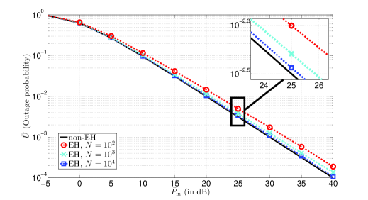
Figure 1: Outage probability for the point-to-point EH and the equivalent non-EH systems for different $N$ and $B_{\rm max}=200\bar{P}_{\rm in}$.

V-C Numerical Results for Example 2

In Fig. 2, we show the average data rate, $\bar{U}$, of the point-to-point EH system discussed in Example 2 in Section II, for different $N$ and $B_{\rm max}=200\bar{P}_{\rm in}$, and compare it to the average data rate of the equivalent non-EH system with average transmit power $\bar{P}_{\rm in}$ and infinite $N$. An ideal transmitter with $\varepsilon=1$ and $P_{\rm C}=0$ is assumed. Fig. 2 shows that even for finite $N$ and finite $B_{\rm max}$, the loss in rate of the point-to-point EH system is small compared to the non-EH system. For $N=10^{2}$, as a performance upper bound, we also show the average rate obtained with the offline solution from [8]. We note that the offline solution, however, needs noncausal knowledge of the harvested powers and the fading gains in all $N=10^{2}$ time slots. In contrast, our proposed solution, although non-optimal for finite $N$, is an online solution and requires only causal knowledge of the fading gain in the current time slot, the average harvested power, and the average fading gain. The optimal online solution for $N=10^{2}$ would result in a curve which is between the curve obtained with the optimal offline solution from [8] and the curve obtained with our proposed solution. However, the optimal online solution for finite $N$ is based on dynamic programing and its exponentially increasing computational complexity becomes prohibitive for $N=10^{2}$.

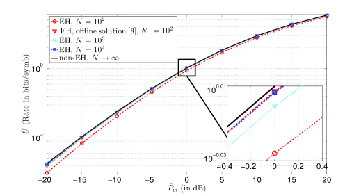
Figure 2: Average rates for the point-to-point EH and the equivalent non-EH systems for different $N$ and $B_{\rm max}=200\bar{P}_{\rm in}$.

In Fig. 3, we plot the average data rate, $\bar{U}$, of a point-to-point EH system for $\varepsilon=5$ and $P_{\rm C}=-25\;{\rm dB}$. We plot $\bar{U}$ for fixed $N=10^{4}$ and different $B_{\rm max}$, and compare it to the average data rate of the non-EH system with an average transmit power $\bar{P}_{\rm in}$ and infinite $N$. The figure shows that, for the adopted $N$, even with $B_{\rm max}=20\bar{P}_{\rm in}$, the loss in rate of the point-to-point EH system is small compared to the non-EH system. We note that in the figure, all rates are zero for $P_{\rm in}\leq-25\;{\rm dB}$ as $P_{\rm C}=-25\;{\rm dB}$.

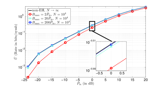
Figure 3: Average rates for the point-to-point EH system and the equivalent non-EH systems for different battery capacity $B_{\rm max}$, and $N=10^{4}$. A realistic transmitter model is adopted with power efficiency $\varepsilon=20$% and constant circuit power consumption $P_{\rm C}=-25$ dB.

V-D Numerical Results for Example 3

In Fig. 4, we plot the rate region of the broadcast EH network with two receivers, cf. Example 3 in Section III, for different $N$, and compare it to the capacity region of the non-EH broadcast network with an average transmit power $\bar{P}_{\rm in}$. For this example, we set $\gamma_{1}=1$, $\gamma_{2}=10$, and $\bar{P}_{\rm in}=10$, cf. Example 3 in Section III. The figure shows that the difference between the rate region of the broadcast EH network with $N=10^{2}$ and the capacity region of the non-EH broadcast network is relatively small and becomes almost negligible for $N=10^{5}$. Hence, indeed as $N\to\infty$, the rate region of the broadcast EH network becomes the capacity region.

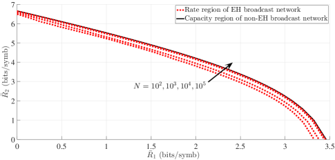
Figure 4: Comparison between the rate region of the broadcast EH network for different $N$, $\gamma_{1}=1$, $\gamma_{2}=10$, and $\bar{P}_{\rm in}=10$, and the capacity region of the non-EH broadcast network with an average transmit power $\bar{P}_{\rm in}=10$.

V-E Numerical Results for Example 4

In Fig. 5, we plot the average data rate, $\bar{U}$, of the multihop relay EH network, considered in Example 4 in Section IV, for $B_{\rm max}=200\bar{P}_{\rm in}$, different $N$, and different numbers of relays, and compare it to the average data rate of the equivalent non-EH relay network with infinite $N$. We assume that $\bar{P}_{{\rm lim},k}=\bar{P}_{\rm in}/2$, for $k=(M-1)/2+1,....,M-1$. Furthermore, we assume that the distance between source and destination is fixed, and that the relays are equidistantly spaced on the line between the source and destination. Hence, if we assume a path loss model with a path loss exponent equal to two, and assume that the fading gains squared have a unit mean, then, for $M-1$ relays between source and destination, the fading gains squared have a mean $M^{2}$. Note that each relay has an average harvested power of $\bar{P}_{\rm in}$. The figure shows that, for fixed $N$, as the number of relays increases, the performance loss of the proposed power allocation solution also increases compared to the performance of the non-EH network. However, as $N$ increases this performance loss becomes negligible as highlighted in Fig. 5 for $N=10^{4}$ and $15$ relays. Hence, even if the utility function $U(i)$ has a relatively complicated form, as is the case in this example, the performance of the proposed online solution for the general EH network is almost identical to the performance of the equivalent non-EH network even for moderate $N$.

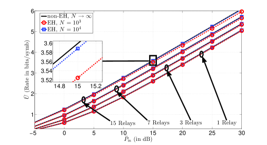
Figure 5: Average rate for multihop relay EH network and equivalent multihop non-EH network for different $N$, $B_{\rm max}=200\bar{P}_{\rm in}$, and different numbers of relays.

VI Conclusion

We have shown that the maximum average performance of an EH network, utilizing optimal online power allocation, converges to the maximum average performance of an equivalent non-EH network with appropriately chosen average transmit power when the number of transmit time slots, $N$, and the battery capacities at each EH node, $B_{\max}$, satisfy $N\to\infty$ and $B_{\max}\to\infty$. We have derived the asymptotically optimal online power allocation which for a general EH network optimizes a general utility function for $N\to\infty$ and $B_{\max}\to\infty$. The considered family of utility functions is general enough to include the most important performance measures in communication theory such as the ergodic data rate, outage probability, average bit error probability, and average signal-to-noise ratio. The optimal online power allocation solution is obtained by solving the power allocation problem of an equivalent non-EH network with nodes having infinite energy available for the transmission of their codewords. Interestingly, the optimal solution only requires knowledge of the average harvested energy but not of the amount of harvested energy in past, present, or future time slots. Although asymptotic in nature, the proposed solution is applicable to EH systems transmitting in a large but finite number of time slots and having nodes with battery capacities much larger than the average harvested power and/or the maximum average transmit power.

-A Proof of Lemma 1

We divide the proof in two parts. In Parts I and II, we consider the cases when $\bar{P}_{\rm d}$ is set to $\bar{P}_{\rm d}=\bar{P}_{\rm lim}<\bar{P}_{\rm in}$ and $\bar{P}_{\rm d}=\bar{P}_{\rm in}\leq\bar{P}_{\rm lim}$, respectively.

-A1 Part I ($\bar{P}_{\rm d}=\bar{P}_{\rm lim}<\bar{P}_{\rm in}$)

Taking the summation $\lim\limits_{N\to\infty}\frac{1}{N}\sum_{i=1}^{N}(\cdot)$ of both sides of (3), we obtain

$$\lim\limits_{N\to\infty}\frac{1}{N}\sum_{i=1}^{N}B(i)=\lim\limits_{N\to\infty}\frac{1}{N}\sum_{i=1}^{N}B(i-1)$$

$$+\lim\limits_{N\to\infty}\frac{1}{N}\sum_{i=1}^{N}P_{\rm in}(i)-\lim\limits_{N\to\infty}\frac{1}{N}\sum_{i=1}^{N}P_{\rm out}(i),$$ (121)

which can be written equivalently as

$$\lim\limits_{N\to\infty}\frac{1}{N}\sum_{i=1}^{N}B(i)-\lim\limits_{N\to\infty}\frac{1}{N}\sum_{i=1}^{N}B(i-1)=\bar{P}_{\rm in}-\bar{P}_{\rm out}.$$ (122)

Now, since $\bar{P}_{\rm d}<\bar{P}_{\rm in}$, and since due to (II-A) $\bar{P}_{\rm out}\leq\bar{P}_{\rm d}$ holds, we have $\bar{P}_{\rm out}<\bar{P}_{\rm in}$, which means that $\bar{P}_{\rm in}-\bar{P}_{\rm out}=\epsilon>0$. Replacing this in the right hand side of (122), and writing $\sum_{i=1}^{N}B(i)=\sum_{i=1}^{N}B(i-1)+B(N)$, where $B(0)=0$, we obtain the following

$$\lim\limits_{N\to\infty}\frac{1}{N}\sum_{i=1}^{N}B(i-1)-\lim\limits_{N\to\infty}\frac{1}{N}\sum_{i=1}^{N}B(i-1)$$

$$+\lim\limits_{N\to\infty}\frac{1}{N}B(N)=\epsilon.$$ (123)

The two sums in (-A1) cancel each other out, and we obtain the following identity for $\bar{P}_{\rm d}=\bar{P}_{\rm lim}<\bar{P}_{\rm in}$

$$\lim\limits_{N\to\infty}B(N)=\lim\limits_{N\to\infty}N\epsilon=\infty.$$ (124)

Hence, when $\bar{P}_{\rm d}=\bar{P}_{\rm lim}<\bar{P}_{\rm in}$ holds, for any time slot $N\to\infty$, (124) holds. This is intuitive, since if in each time slot, on average, more energy is stored in an infinite storage battery than what is extracted from the battery, then, after $N\to\infty$ time slots, there must be infinite energy in the battery. We now use (124) for proving the following proposition.

Proposition 1

When $\bar{P}_{\rm d}=\bar{P}_{\rm lim}<\bar{P}_{\rm in}$, there must be some time slot, denoted by $j$, after which for any $i>j$ the event $P_{\rm out}(i)=\min\{B(i-1),P_{\rm d}(i)\}=B(i-1)$ does not occur, and for $i>j$, only the event $P_{\rm out}(i)=\min\{B(i-1),P_{\rm d}(i)\}=P_{\rm d}(i)$ occurs. Moreover, $j$ must satisfy

$$\lim_{N\to\infty}\frac{j}{N}=0.$$ (125)

Proof of Proposition 1: We prove Proposition 1 by contradiction. Hence, we assume that we cannot find a time slot $j$, defined in Proposition 1, since $\min\{B(j-1),P_{\rm d}(j)\}=B(j-1)$ occurred for some large $j$ for which $\lim\limits_{N\to\infty}j/N\neq 0$ holds. However, if $\lim\limits_{N\to\infty}j/N\neq 0$ holds, then $j\to\infty$ must hold. Consequently, if $j\to\infty$ and $\min\{B(j-1),P_{\rm d}(j)\}=B(j-1)$ occurred for that $j$, then due to (124) we would get the following identity

$$\lim_{j\to\infty}\min\{B(j-1),P_{\rm d}(j)\}=\lim_{j\to\infty}B(j-1)=\infty.$$ (126)

However, since the power $P_{\rm d}(j)$ is finite, the expression in the left hand side of (126) must also satisfy

$$\lim_{j\to\infty}\min\{B(j-1),P_{\rm d}(j)\}\leq\lim_{j\to\infty}P_{\rm d}(j)<\infty,$$ (127)

which is a contradiction to (126), i.e., we obtain that for $j\to\infty$ both (126) and (127) have to hold, which is impossible. As a result, Proposition 1 must be true.

Now if Proposition 1 is true, then the number of time slots $\Delta$ for which $P_{\rm out}(i)\neq P_{\rm d}(i)$ holds, satisfies $\lim_{N\to\infty}\Delta/N=0$, and the number of time slots for which $P_{\rm out}(i)=P_{\rm d}(i)$ holds satisfies $\lim_{N\to\infty}(N-\Delta)/N=1$. Thereby, $P_{\rm out}(i)=P_{\rm d}(i)$ holds practically always. This concludes the proof that $P_{\rm out}(i)=P_{\rm d}(i)$ holds practically always.

On the other hand, since $P_{\rm d}(i)$ and $U(i)$, $\forall i$, are finite, and since $j$ is finite, we have

$$\lim_{N\to\infty}\frac{1}{N}\sum_{i=1}^{j}P_{\rm d}(i)=0$$ (128)

$$\lim_{N\to\infty}\frac{1}{N}\sum_{i=1}^{j}\min\{B(i-1),P_{\rm d}(i)\}=0$$ (129)

$$\lim_{N\to\infty}\frac{1}{N}\sum_{i=1}^{j}U(i)=0.$$ (130)

From (128)-(130), we obtain the following

$$\bar{P}_{\rm out} =\lim_{N\to\infty}\frac{1}{N}\sum_{i=1}^{j}\min\{B(i-1),P_{\rm d}(i)\}$$

$$+\lim_{N\to\infty}\frac{1}{N}\sum_{i=j+1}^{N}P_{\rm d}(i)=\bar{P}_{\rm d}.$$ (131)

$$\bar{U} =\lim_{N\to\infty}\frac{1}{N}\sum_{i=1}^{j}U(i)+\lim_{N\to\infty}\frac{1}{N}\sum_{i=j+1}^{N}U(i)$$

$$=\lim_{N\to\infty}\frac{1}{N}\sum_{i=j+1}^{N}U(i),$$ (132)

i.e., $\bar{P}_{\rm out}=\bar{P}_{\rm d}$ and only the codewords after the $j$-th slot contribute to the average utility function, the contribution of the other codewords is negligible. Since for $i>j$, $P_{\rm out}(i)=P_{\rm d}(i)$ holds always, we obtain that only the codewords for which $P_{\rm out}(i)=P_{\rm d}(i)$ holds contribute to the average utility function $\bar{U}$ and the other codewords have negligible contributions to $\bar{U}$. This completes the proof of Part I.

-A2 Part II ($\bar{P}_{\rm d}=\bar{P}_{\rm in}\leq\bar{P}_{\rm lim}$)

If $\bar{P}_{\rm d}=\bar{P}_{\rm in}$, the following must hold

$$\bar{P}_{\rm out} =\lim_{N\to\infty}\frac{1}{N}\sum_{i=1}^{N}\min\{B(i-1),P_{\rm d}(i)\}$$

$$=\lim_{N\to\infty}\frac{1}{N}\sum_{i=1}^{N}P_{\rm d}(i)=\bar{P}_{\rm d}=\bar{P}_{\rm in}.$$ (133)

We prove the above claim by contradiction. Assume that $\bar{P}_{\rm d}=\bar{P}_{\rm in}$ holds, however, (-A2) does not hold and

$$\bar{P}_{\rm out} =\lim_{N\to\infty}\frac{1}{N}\sum_{i=1}^{N}\min\{B(i-1),P_{\rm d}(i)\}$$

$$<\lim_{N\to\infty}\frac{1}{N}\sum_{i=1}^{N}P_{\rm d}(i)=\bar{P}_{\rm d}=\bar{P}_{\rm in}$$ (134)

holds instead. However, since $\bar{P}_{\rm out}<\bar{P}_{\rm in}$ holds, according to the proof in Part I, $\bar{P}_{\rm out}$ has to be given by (131). Thereby, we obtain a contradiction that both (131) and (-A2) must hold. Due to this contradiction, (-A2) cannot hold and (-A2) must hold instead. This concludes the proof of (-A2).

Now, there are only two cases for which (-A2) can hold. The first case is when the number of slots for which $P_{\rm out}(i)=B(i-1)$ holds, denoted by $\Delta$, is negligible compared to the number of slots for which $P_{\rm out}(i)=P_{\rm d}(i)$ holds, i.e., $\Delta$ is such that $\lim_{N\to\infty}{\Delta}/N=0$ holds. As a result, the codewords for which $P_{\rm out}(i)=B(i-1)$ occurs have negligible effect on the average utility function $\bar{U}$ compared to the codewords for which $P_{\rm out}(i)=P_{\rm d}(i)$ occurs. This can be proved as follows. Put all time slots $i$ for which $P_{\rm out}(i)=B(i-1)$ occurs into set $\mathcal{I}$ and the rest of time slots for which $P_{\rm out}(i)=P_{\rm d}(i)$ occurs into set $\bar{\mathcal{I}}$ . Then, let $U_{\max}=\max_{i\in\mathcal{I}}U(i)$. Since $U_{\max}$ is finite it follows that the contribution of the codewords with powers $P_{\rm out}(i)=B(i-1)$ to the average utility function is

$$\lim_{N\to\infty}\frac{1}{N}\sum_{i\in\mathcal{I}}U(i)\leq\lim_{N\to\infty}\frac{1}{N}\sum_{i\in\mathcal{I}}U_{\max}$$

$$=\lim_{N\to\infty}\frac{\Delta}{N}\times U_{\max}=0.$$ (135)

The second case is when the number of slots for which $P_{\rm out}(i)=B(i-1)$ holds, $\Delta$, is not negligible compared to the number of slots for which $P_{\rm out}(i)=P_{\rm d}(i)$ holds, i.e., $\Delta$ is such that $\lim_{N\to\infty}{\Delta}/N>0$ holds. Nevertheless, we can prove when $P_{\rm out}(i)=B(i-1)$ occurs, the difference between $B(i-1)$ and $P_{\rm d}(i)$ must be so small that its effect on $\bar{U}$ is negligible. As a result of this negligible effect on $\bar{U}$, we can assume that $P_{\rm out}(i)=B(i-1)=P_{\rm d}(i)$ holds for practically all time slots. This is proven in the following.

Since (-A2) holds, using the sets $\mathcal{I}$ and $\bar{\mathcal{I}}$, we can rewrite (-A2) as

$$\lim_{N\to\infty}\frac{1}{N}\sum_{i=1}^{N}P_{\rm d}(i) =\lim_{N\to\infty}\frac{1}{N}\sum_{i\in\mathcal{I}}^{N}B(i-1)$$

$$+\lim_{N\to\infty}\frac{1}{N}\sum_{i\in\bar{\mathcal{I}}}^{N}P_{\rm d}(i).$$ (136)

Substracting the right hands side of (-A2) from both sides of (-A2), we obtain that

$$\lim_{N\to\infty}\frac{1}{N}\sum_{i\in\mathcal{I}}^{N}\big{(}P_{\rm d}(i)-B(i-1)\big{)}=0$$ (137)

must hold. Now, since for $i\in\mathcal{I}$, $P_{\rm d}(i)>B(i-1)$ holds, we can conclude that (137) can hold if and only if in almost all time slots $i\in\mathcal{I}$, the difference between $P_{\rm d}(i)$ and $B(i-1)$ is negligible. Or, more precisely, for $i\in\mathcal{I}$, the average of the difference

$$\epsilon(i)=P_{\rm d}(i)-B(i-1)>0,\;\;i\in\mathcal{I},$$ (138)

satisfies

$$\lim_{N\to\infty}\frac{1}{N}\sum_{i\in\mathcal{I}}^{N}\epsilon(i)=0.$$ (139)

In the following, we prove that the events in which $P_{\rm out}(i)=B(i-1)$ occurs have negligible effect on $\bar{U}$. To this end, let us define $\bar{U}_{\rm d}$ as the average utility function obtained when $P_{\rm out}(i)=P_{\rm d}(i)$, $\forall i$. Then, we can write $\bar{U}_{\rm d}$ and $\bar{U}$

$$\bar{U}_{\rm d} =\lim_{N\to\infty}\frac{1}{N}\sum_{i=1}^{N}U(P_{\rm d}(i))$$

$$=\lim_{N\to\infty}\frac{1}{N}\sum_{i\in\mathcal{I}}U(P_{\rm d}(i))+\lim_{N\to\infty}\frac{1}{N}\sum_{i\in\bar{\mathcal{I}}}U(P_{\rm d}(i))$$ (140)

$$\bar{U} =\lim_{N\to\infty}\frac{1}{N}\sum_{i=1}^{N}U(P_{\rm out}(i))$$

$$=\lim_{N\to\infty}\frac{1}{N}\sum_{i\in\mathcal{I}}U(B(i-1))+\lim_{N\to\infty}\frac{1}{N}\sum_{i\in\bar{\mathcal{I}}}U(P_{\rm d}(i)).$$ (141)

Now, using (138), we can obtain $P_{\rm d}(i)$ for $i\in\mathcal{I}$ as $P_{\rm d}(i)=B(i-1)+\epsilon(i)$. Inserting this into (140) we can obtain $\bar{U}_{\rm d}$ as

$$\bar{U}_{\rm d}=$$

$$\lim_{N\to\infty}\frac{1}{N}\sum_{i\in\mathcal{I}}U(B(i-1)+\epsilon(i))+\lim_{N\to\infty}\frac{1}{N}\sum_{i\in\bar{\mathcal{I}}}U(P_{\rm d}(i))$$

$$\stackrel{{\scriptstyle(a)}}{{=}}\lim_{N\to\infty}\frac{1}{N}\sum_{i\in\mathcal{I}}U(B(i-1))+\lim_{N\to\infty}\frac{1}{N}\sum_{i\in\bar{\mathcal{I}}}U(P_{\rm d}(i))=\bar{U},$$ (142)

where $(a)$ follows from the fourth property of $\bar{U}$ given in Definition 1.

Hence, also for the second part when $\bar{P}_{\rm d}=\bar{P}_{\rm in}\leq\bar{P}_{\rm lim}$ holds, we can conclude that $P_{\rm out}(i)=P_{\rm d}(i)$ holds for practically all time slots. This completes the proof of Lemma 1.

-B Proof of Theorem 2

Following the same procedure as for the proofs in Appendix -A, with $\bar{P}_{\rm d}$ adjusted to $\bar{P}_{\rm d}=\min\{\bar{P}_{\rm lim},\bar{P}_{\rm in}\}$, we obtain that $P_{\rm out}(i)=P_{\rm d}(i)$ holds for practically all time slots when $N\to\infty$. Now, for each time slot $i$ for which $P_{\rm out}(i)=P_{\rm d}(i)$ holds, $P_{{\rm out},k}(i)=P_{{\rm d},k}(i)$, $\forall k$, also holds. Therefore, it follows that $P_{{\rm out},k}(i)=P_{{\rm d},k}(i)$, $\forall k$, holds for practically all time slots when $N\to\infty$. Consequently, following the method in the proof of Theorem 1, we can write (46) as (51) with appropriately adjusted $P_{\rm lim,non-EH}=\min\{\bar{P}_{\rm lim},\bar{P}_{\rm in}\}$ as explained in Theorem 2.

-C Proof of Theorem 3

In this proof, set $\mathcal{A}$ comprises the indices of the nodes with $\bar{P}_{{\rm lim},k}<\bar{P}_{{\rm in},k}$ and set $\bar{\mathcal{A}}$ comprises the indices of the nodes with $\bar{P}_{{\rm lim},k}\geq\bar{P}_{{\rm in},k}$. We first prove that for the nodes $k\in\mathcal{A}$, the number of time slots for which $P_{{\rm out},k}(i)\neq P_{{\rm d},k}(i)$ holds is negligible compared to the number of time slots with $P_{{\rm out},k}(i)=P_{{\rm d},k}(i)$. To this end, we use the proof in Appendix -A, where it is shown that an individual node $k\in\mathcal{A}$, after some finite number of time slots $j_{k}$, transmits with power $P_{{\rm out},k}(i)=P_{{\rm d},k}(i)$, $\forall i>j_{k}$, where $\lim_{N\to\infty}j_{k}/N=0$. Now, let $j=\max_{k}\{j_{k}\}$. Then, $\lim_{N\to\infty}j/N=0$ holds. Furthermore, after this $j$-th time slot, all of the nodes $k\in\mathcal{A}$ transmit with power $P_{{\rm out},k}(i)=P_{{\rm d},k}(i)$, $\forall i>j$, i.e., these nodes transmit with power $P_{{\rm out},k}(i)=P_{{\rm d},k}(i)$ for practically all time slots. This completes the proof for the nodes in the set set $\mathcal{A}$. Now, we are only left to prove that for the nodes $k\in\bar{\mathcal{A}}$, the number of time slots in which $P_{{\rm out},k}(i)\neq P_{{\rm d},k}(i)$ holds is negligible compared to the number of time slots with $P_{{\rm out},k}(i)=P_{{\rm d},k}(i)$. To this end, for each node $k\in\bar{\mathcal{A}}$, let us create a set $\mathcal{I}_{k}$ in which we put the time slots $i$ for which $P_{{\rm out},k}(i)\neq P_{{\rm d},k}(i)$ holds. Furthermore, let us create the set $\mathcal{I}$ in which we put the time slots $i$ for which $P_{{\rm out},k}(i)\neq P_{{\rm d},k}(i)$ holds for at least one of the nodes $k\in\bar{\mathcal{A}}$, i.e., $\mathcal{I}$ is the union of all $\mathcal{I}_{k}$ for $k\in\bar{\mathcal{A}}$. Thereby, the cardinality of $\mathcal{I}$ is upper bounded by the sum of the cardinalities of $\mathcal{I}_{k}$, $\forall k\in\bar{\mathcal{A}}$, i.e., the cardinality of $\mathcal{I}$, denoted by $\Delta$, is upper bounded as

$$\Delta=|\mathcal{I}|\leq\sum_{k\in\bar{\mathcal{A}}}|\mathcal{I}_{k}|.$$ (143)

According to the proof in Appendix -A, if $\bar{P}_{{\rm d},k}=\bar{P}_{{\rm in},k}$ holds, for any individual node $k$, $P_{{\rm out},k}(i)=P_{{\rm d},k}(i)$ hold for practically all time slots. Hence, let us adopt $\bar{P}_{{\rm d},k}=\bar{P}_{{\rm in},k}$, $\forall k\in\mathcal{\bar{A}}$. Now, since $|\mathcal{I}_{k}|$ is the number of time slots in which $P_{{\rm out},k}(i)\neq P_{{\rm d},k}(i)$ holds for node $k\in\mathcal{\bar{A}}$, according to the proof in Appendix -A, $|\mathcal{I}_{k}|$ satisfies

$$\lim_{N\to\infty}|\mathcal{I}_{k}|/N=0\;,\forall k\in\bar{\mathcal{A}}.$$ (144)

Now, combining (143) and (144) we find that the cardinality of $\mathcal{I}$ satisfies

$$\lim_{N\to\infty}\Delta/N\leq\sum_{k\in\bar{\mathcal{A}}}\lim_{N\to\infty}|\mathcal{I}_{k}|/N=0.$$ (145)

when $|\mathcal{\bar{A}}|<\infty$. Therefore, the cumulative effect of $P_{{\rm out},k}(i)\neq P_{{\rm d},k}(i)$ on $\bar{U}$ from the nodes in $\mathcal{A}$ and $\mathcal{\bar{A}}$ is negligible since $\lim_{N\to\infty}(j+\Delta)/N=0$ holds. Therefore, following the method in the proof of Theorem 1, we can write (61) as (66) with appropriately adjusted $P_{\rm lim,non-EH}$ as explained in Theorem 3. This completes the proof.

-D Proof of Theorem 4

The proof for the general EH network is identical to that of the multiple-access EH network given in Appendix -C, however, the powers $P_{{\rm out},k}(i)$ and $P_{{\rm d},k}(i)$ now have different meanings and are given by (82) and (83), respectively. In particular, $P_{{\rm out},k}(i)$ and $P_{{\rm d},k}(i)$ now are the total transmit and the total desired powers in time slot $i$ of the $k$-th EH transmit node to all receiving nodes. Hence, by following the same procedure as for the proof in Appendix -C, we can prove that, if for the nodes $k\in\mathcal{A}$ for which $\bar{P}_{{\rm lim},k}<\bar{P}_{{\rm in},k}$ holds and the nodes $k\in\bar{\mathcal{A}}$ for which $\bar{P}_{{\rm lim},k}\geq\bar{P}_{{\rm in},k}$ holds, $\bar{P}_{{\rm d},k}$ is set to $\bar{P}_{{\rm d},k}=\bar{P}_{{\rm lim},k}$ and $\bar{P}_{{\rm d},k}=\bar{P}_{{\rm in},k}$, respectively, we obtain that $P_{{\rm out},k}(i)=P_{{\rm d},k}(i)$ holds for practically all time slots. As a result, $P_{{\rm out},k\to j}(i)=P_{{\rm d},k\to j}(i)$ also holds $\forall i,k,j$. Hence, Theorem 4 follows.

Nikola Zlatanov (S’06, M’15) was born in Macedonia. He received the Dipl.Ing. and Master degree in electrical engineering from Ss. Cyril and Methodius University, Skopje, Macedonia in 2007 and 2010, respectively, and his PhD degree from the University of British Columbia (UBC) in Vancouver, Canada in 2015. He is currently a Lecturer (Assistant Professor) in the Department of Electrical and Computer Systems Engineering at Monash University in Melbourne, Australia. His current research interests include wireless communications and information theory. Dr. Zlatanov received several scholarships/awards for his work including UBC’s Four Year Doctoral Fellowship in 2010, UBC’s Killam Doctoral Scholarship and Macedonia’s Young Scientist of the Year in 2011, the Vanier Canada Graduate Scholarship in 2012, best journal paper award from the German Information Technology Society (ITG) in 2014, and best conference paper award at ICNC in 2016. Dr. Zlatanov serves as an Editor of IEEE Communications Letters. He has been a TPC member of various conferences, including Globecom, ICC, VTC, and ISWCS.

Robert Schober (S’98, M’01, SM’08, F’10) was born in Neuendettelsau, Germany, in 1971. He received the Diplom (Univ.) and the Ph.D. degrees in electrical engineering from the University of Erlangen-Nuermberg in 1997 and 2000, respectively. From May 2001 to April 2002 he was a Postdoctoral Fellow at the University of Toronto, Canada, sponsored by the German Academic Exchange Service (DAAD). From 2002 to 2011, he was a Professor and Canada Research Chair at the University of British Columbia (UBC), Vancouver, Canada. Since January 2012 he is an Alexander von Humboldt Professor and the Chair for Digital Communication at the Friedrich Alexander University (FAU), Erlangen, Germany. His research interests fall into the broad areas of Communication Theory, Wireless Communications, and Statistical Signal Processing. Dr. Schober received several awards for his work including the 2002 Heinz Maier Leibnitz Award of the German Science Foundation (DFG), the 2004 Innovations Award of the Vodafone Foundation for Research in Mobile Communications, the 2006 UBC Killam Research Prize, the 2007 Wilhelm Friedrich Bessel Research Award of the Alexander von Humboldt Foundation, the 2008 Charles McDowell Award for Excellence in Research from UBC, a 2011 Alexander von Humboldt Professorship, and a 2012 NSERC E.W.R. Steacie Fellowship. In addition, he has received several best paper awards for his research. Dr. Schober is a Fellow of the Canadian Academy of Engineering and a Fellow of the Engineering Institute of Canada. From 2012 to 2015, he served as Editor-in-Chief of the IEEE Transactions on Communications and since 2014, he is the Chair of the Steering Committee of the IEEE Transactions on Molecular, Biological and Multiscale Communication. Furthermore, he is a Member at Large of the Board of Governors of the IEEE Communications Society.

Zoran Hadzi-Velkov (M’97, SM’11) received Dipl.-Ing. in electrical engineering (honors), Magister Ing. in communications engineering (honors), and Ph.D. in technical sciences from the Ss. Cyril and Methodius University in Skopje, Macedonia, in 1996, 2000, and 2003, respectively. He is currently a Professor of telecommunications at his alma mater. During 2001 and 2002, he was a visiting scholar at the IBM Watson Research Center, New York, USA. Between 2012 and 2014, Dr. Hadzi-Velkov was a visiting professor at the Institute for Digital Communications, University of Erlangen-Nuremberg in Germany. He received the Alexander von Humboldt fellowship for experienced researchers in 2012, and the annual best scientist award from Ss. Cyril and Methodius University in 2014. Between 2012 and 2015, he was the Chair of the Macedonian Chapter of IEEE Communications Society. He has served on the technical program committees of numerous international conferences, including IEEE ICC 2013, IEEE ICC 2014, IEEE ICC 2015, IEEE GLOBECOM 2015, and IEEE GLOBECOM 2016. Since 2012, Dr. Hadzi-Velkov served as an Editor for IEEE COMMUNICATIONS LETTERS. His research interests are in the broad area of wireless communications, with particular emphasis on cooperative communications, green communications, and energy harvesting communications.

References

- [1] N. Zlatanov, Z. Hadzi-Velkov, and R. Schober, “Asymptotically Optimal Power Allocation for Point-to-Point Energy Harvesting Communication Systems,” in IEEE Global Commun. Conf. (GLOBECOM), Dec. 2013, pp. 2502–2507.
- [2] G. Ottman, H. Hofmann, A. Bhatt, and G. Lesieutre, “Adaptive Piezoelectric Energy Harvesting Circuit for Wireless Remote Power Supply,” IEEE Trans. on Power Electronics, vol. 17, pp. 669–676, Sep. 2002.
- [3] P. Mitcheson, E. Yeatman, G. Rao, A. Holmes, and T. Green, “Energy Harvesting from Human and Machine Motion for Wireless Electronic Devices,” Proceedings of the IEEE, vol. 96, pp. 1457–1486, Sep. 2008.
- [4] J. Paradiso and T. Starner, “Energy Scavenging for Mobile and Wireless Electronics,” IEEE Pervasive Computing, vol. 4, pp. 18–27, Jan. 2005.
- [5] S. Ulukus, A. Yener, E. Erkip, O. Simeone, M. Zorzi, P. Grover, and K. Huang, “Energy Harvesting Wireless Communications: A Review of Recent Advances,” IEEE J. Select. Areas Commun., vol. 33, pp. 360–381, Mar. 2015.
- [6] O. Ozel, K. Tutuncuoglu, S. Ulukus, and A. Yener, “Fundamental limits of energy harvesting communications,” IEEE Communications Magazine, vol. 53, pp. 126–132, April 2015.
- [7] M. L. Ku, W. Li, Y. Chen, and K. J. R. Liu, “Advances in Energy Harvesting Communications: Past, Present, and Future Challenges,” IEEE Commun. Surveys Tutorials, vol. 18, no. 2, pp. 1384–1412, Second quarter 2016.
- [8] C. K. Ho and R. Zhang, “Optimal Energy Allocation for Wireless Communications with Energy Harvesting Constraints,” IEEE Trans. Signal Processing, vol. 60, pp. 4808–4818, Sep. 2012.
- [9] O. Ozel, K. Tutuncuoglu, J. Yang, S. Ulukus, and A. Yener, “Transmission with Energy Harvesting Nodes in Fading Wireless Channels: Optimal Policies,” IEEE J. Select. Areas Commun., vol. 29, pp. 1732–1743, Sep. 2011.
- [10] V. Sharma, U. Mukherji, V. Joseph, and S. Gupta, “Optimal Energy Management Policies for Energy Harvesting Sensor Nodes,” IEEE Trans. Wireless Commun., vol. 9, pp. 1326–1336, Apr. 2010.
- [11] J. Yang, O. Ozel, and S. Ulukus, “Broadcasting with an Energy Harvesting Rechargeable Transmitter,” IEEE Trans. Wireless Commun., vol. 11, pp. 571–583, Feb. 2012.
- [12] X. Wang, Z. Nan, and T. Chen, “Optimal MIMO Broadcasting for Energy Harvesting Transmitter With non-Ideal Circuit Power Consumption,” IEEE Trans. Wireless Commun., vol. 14, pp. 2500–2512, May 2015.
- [13] M. Antepli, E. Uysal-Biyikoglu, and H. Erkal, “Optimal Packet Scheduling on an Energy Harvesting Broadcast Link,” IEEE J. Select. Areas Commun., vol. 29, pp. 1721–1731, Sep. 2011.
- [14] O. Ozel, J. Yang, and S. Ulukus, “Optimal Broadcast Scheduling for an Energy Harvesting Rechargeable Transmitter with a Finite Capacity Battery,” IEEE Trans. Wireless Commun., vol. 11, no. 6, pp. 2193–2203, 2012.
- [15] ——, “Optimal Scheduling Over Fading Broadcast Channels With an Energy Harvesting Transmitter,” in 4th IEEE International Workshop on Computational Advances in Multi-Sensor Adaptive Processing (CAMSAP), 2011, pp. 193–196.
- [16] J. Yang and S. Ulukus, “Optimal Packet Scheduling in a Multiple Access Channel with Energy Harvesting Transmitters,” Journal of Communications and Networks, vol. 14, pp. 140–150, Apr. 2012.
- [17] Z. Wang, V. Aggarwal, and X. Wang, “Iterative Dynamic Water-Filling for Fading Multiple-Access Channels With Energy Harvesting,” IEEE J. Select. Areas Commun., vol. 33, pp. 382–395, Mar. 2015.
- [18] R. A. Raghuvir, D. Rajan, and M. D. Srinath, “Capacity of the Multiple Access Channel in Energy Harvesting Wireless Networks,” in IEEE Wireless Communications and Networking Conference (WCNC), 2012, pp. 898–902.
- [19] C. Huang, R. Zhang, and S. Cui, “Throughput Maximization for the Gaussian Relay Channel with Energy Harvesting Constraints,” IEEE J. Select. Areas Commun., vol. 31, pp. 1469–1479, Aug. 2013.
- [20] B. Medepally and N. Mehta, “Voluntary Energy Harvesting Relays and Selection in Cooperative Wireless Networks,” IEEE Trans. Wireless Commun., vol. 9, Nov. 2010.
- [21] A. Minasian, S. ShahbazPanahi, and R. Adve, “Energy Harvesting Cooperative Communication Systems,” IEEE Trans. Wireless Commun., vol. 13, pp. 6118–6131, Nov. 2014.
- [22] I. Ahmed, A. Ikhlef, R. Schober, and R. Mallik, “Joint Power Allocation and Relay Selection in Energy Harvesting AF Relay Systems,” IEEE Wireless Commun. Lett., vol. 2, pp. 239–242, Apr. 2013.
- [23] A. Fouladgar and O. Simeone, “On the Transfer of Information and Energy in Multi-User Systems,” IEEE Commun. Lett., vol. 16, pp. 1733–1736, Nov. 2012.
- [24] C. Huang, R. Zhang, and S. Cui, “Optimal Power Allocation for Outage Probability Minimization in Fading Channels with Energy Harvesting Constraints,” IEEE Trans. Wireless Commun., vol. 13, pp. 1074–1087, Feb. 2014.
- [25] S. Zhou, T. Chen, W. Chen, and Z. Niu, “Outage Minimization for a Fading Wireless Link With Energy Harvesting Transmitter and Receiver,” IEEE J. Select. Areas Commun., vol. 33, pp. 496–511, Mar. 2015.
- [26] O. Ozel and S. Ulukus, “Achieving AWGN Capacity Under Stochastic Energy Harvesting,” IEEE Trans. Inform. Theory, vol. 58, no. 10, pp. 6471–6483, 2012.
- [27] A. Goldsmith and P. Varaiya, “Capacity of Fading Channels with Channel Side Information,” IEEE Trans. Inform. Theory, vol. 43, pp. 1986–1992, Nov. 1997.
- [28] G. Caire, G. Taricco, and E. Biglieri, “Optimum Power Control over Fading Channels,” IEEE Trans. Inform. Theory, vol. 45, pp. 1468–1489, Jul. 1999.
- [29] O. Arnold, F. Richter, G. Fettweis, and O. Blume, “Power Consumption Modeling of Different Base Station Types in Heterogeneous Cellular Networks,” in Future Network and Mobile Summit, 2010, pp. 1–8.
- [30] D. Ng, E. Lo, and R. Schober, “Wireless Information and Power Transfer: Energy Efficiency Optimization in OFDMA Systems,” IEEE Trans. Wireless Commun., vol. 12, pp. 6352–6370, Dec. 2013.
- [31] T. M. Cover and J. A. Thomas, Elements of Information Theory. Wiley-interscience, 2006.
- [32] M. Hasna and M.-S. Alouini, “Outage Probability of Multihop Transmission Over Nakagami Fading Channels,” IEEE Comm. Letters, vol. 7, pp. 216–218, 2003.