Convergence of Gaussian quasi-likelihood random fields for ergodic Lévy driven SDE observed at high frequency

Abstract

This paper investigates the Gaussian quasi-likelihood estimation of an exponentially ergodic multidimensional Markov process, which is expressed as a solution to a Lévy driven stochastic differential equation whose coefficients are known except for the finite-dimensional parameters to be estimated, where the diffusion coefficient may be degenerate or even null. We suppose that the process is discretely observed under the rapidly increasing experimental design with step size $h_{n}$. By means of the polynomial-type large deviation inequality, convergence of the corresponding statistical random fields is derived in a mighty mode, which especially leads to the asymptotic normality at rate $\sqrt{nh_{n}}$ for all the target parameters, and also to the convergence of their moments. As our Gaussian quasi-likelihood solely looks at the local-mean and local-covariance structures, efficiency loss would be large in some instances. Nevertheless, it has the practically important advantages: first, the computation of estimates does not require any fine tuning, and hence it is straightforward; second, the estimation procedure can be adopted without full specification of the Lévy measure.

t1Supported in part by JSPS KAKENHI Grant Number 20740061 and 23740082.

1 Introduction

Let $X=(X_{t})_{t\in\mathbb{R}_{+}}$ be a solution to the stochastic differential equation (SDE)

$$dX_{t}=a(X_{t},\alpha)\,dt+b(X_{t},\beta)\,dW_{t}+c(X_{t-},\beta)\,dJ_{t},$$ (1)

where the ingredients involved are as follows:

• the finite-dimensional unknown parameter

  $$\theta=(\alpha,\beta)\in\Theta_{\alpha}\times\Theta_{\beta}=:\Theta,$$

  where, for simplicity, the parameter spaces $\Theta_{\alpha}\subset\mathbb{R}^{p_{\alpha}}$ and $\Theta_{\beta}\subset\mathbb{R}^{p_{\beta}}$ are supposed to be bounded convex domains; the parameter $\alpha$ (resp., $\beta$) affects local trend (resp., local dispersion);

• an $r^{\prime}$-dimensional standard Wiener process $W$ and an $r^{\prime\prime}$-dimensional centered pure-jump Lévy process $J$, whose Lévy measure is denoted by $\nu$;

• the initial variable $X_{0}$ independent of $(W,J)$, with $\eta:=\mathcal{L}(X_{0})$ possibly depending on $\theta$;

• the measurable functions $a\dvtx\mathbb{R}^{d}\times\Theta_{\alpha}\to\mathbb{R}^{d}$, $b\dvtx\mathbb{R}^{d}\times\Theta_{\beta}\to\mathbb{R}^{d}\otimes\mathbb{R}^{r^{\prime}}$, and $c\dvtx\mathbb{R}^{d}\times\Theta_{\beta}\to\mathbb{R}^{d}\otimes\mathbb{R}^{r^{\prime\prime}}$.

Incorporation of the jump part extends the continuous-path diffusion parametric model, which are nowadays widely used in many application fields. We denote by $P_{\theta}$ the image measure of a solution process $X$ associated with $\theta\in\Theta\subset\mathbb{R}^{p}$, where $p:=p_{\alpha}+p_{\beta}$. Suppose that the true parameter $\theta_{0}=(\alpha_{0},\beta_{0})\in\Theta$ does exist, with $P_{0}$ denoting the shorthand for the true image measure $P_{\theta_{0}}$, and that $X$ is not completely (continuously) observed but only discretely at high frequency under the condition for the rapidly increasing experimental design: we are given a sample $(X_{t_{0}},X_{t_{1}},\ldots,X_{t_{n}})$, where $t_{j}=t^{n}_{j}=jh_{n}$ for some $h_{n}>0$ such that

$$T_{n}:=nh_{n}\to\infty\quad\mbox{and}\quad nh_{n}^{2}\to 0$$ (2)

for $n\to\infty$. The main objective of this paper is to estimate $\theta_{0}$ under the exponential ergodicity of $X$; the equidistant sampling assumption can be weakened to some extent as long as the long-term and high-frequency framework is concerned; however, it is just a technical extension making the presentation notationally messy, and hence we do not deal with it in the main context to make the presentation more clear.

It is common knowledge that the maximum likelihood estimation is generally infeasible, since the transition probability is most often unavailable in a closed form. This implies that the conventional statistical analyses based on the genuine likelihood have no utility. For this reason, we have to resort to some other feasible estimation procedure, which could be a lot of things. Among several possibilities, we are concerned here with the Gaussian quasi-likelihood (GQL) function defined as if the conditional distributions of $X_{t_{j}}$ given $X_{t_{j-1}}$ are Gaussian with approximate but explicit mean vector and covariance matrix; see (11) below.

The terminology “quasi-likelihood” has originated as the pioneering work of Wedderburn Wed74 , the concept of which formed a basis of the generalized linear regression. The GQL-based estimation has been known to have the advantage of computational simplicity and robustness for misspecification of the noise distribution, and is well-established as a fundamental tool in estimating possibly non-Gaussian and dependent statistical models. Just to be a little more precise, consider a time-series $Y_{1},\ldots,Y_{n}$ in $\mathbb{R}$ with a fixed $Y_{0}$, and denote by $m_{j-1}(\theta)\in\mathbb{R}$ and $v_{j-1}(\theta)>0$ the conditional mean and conditional variance of $Y_{j}$ given $(Y_{0},\ldots,Y_{j-1})$, where $\theta$ is an unknown parameter of interest. Then, the Gaussian quasi maximum likelihood estimator (GQMLE) is defined to be a maximizer of the function

$$\theta\mapsto\sum_{j=1}^{n}\log\biggl{\{}\frac{1}{\sqrt{2\pi v_{j-1}(\theta)}}\exp\biggl{(}-\frac{(Y_{j}-m_{j-1}(\theta))^{2}}{2v_{j-1}(\theta)}\biggr{)}\biggr{\}}.$$

Namely, we compute the likelihood of $(Y_{1},Y_{2},\ldots,Y_{n})$ as if the conditional law of $Y_{j}$ given $(Y_{1},\ldots,Y_{j-1})$ is Gaussian with mean $m_{j-1}(\theta)$ and variance $v_{j-1}(\theta)$, so that only the structures of the conditional mean and variance do matter. Although it is not asymptotically efficient in general, it can serve as a widely applicable estimation procedure. One can consult Heyde Hey97 for an extensive and systematic account of statistical inference based on the GQL. The GQL has been a quite popular tool for (semi)parametric estimation, and especially there exists a vast amount of literature concerning asymptotics of the GQL for time series models with possibly non-Gaussian error sequence; among others, we refer to Straumann and Mikosch StrMik06 for a class of conditionally heteroscedastic time series models, and Bardet and Wintenburger BarWin09 for multidimensional causal time series, as well as the references therein.

Let us return to our framework. On one hand, for the diffusion case (where $c\equiv 0$), the GQL-estimation issue has been solved under some regularity conditions, especially the GQL, which leads to an asymptotically efficient estimator, where the crucial point is that the optimal rates of convergence for estimating $\alpha$ and $\beta$ are different and given by $\sqrt{T_{n}}$ and $\sqrt{n}$, respectively; see Gobet Gob02 for the local asymptotic normality of the corresponding statistical experiments. For how to construct an explicit contrast function, we refer to Yoshida Yos92 and Kessler Kes97 as well as the references therein; specifically, they employed a discretized version of the continuous-observation likelihood process, and a higher order local-Gauss approximation of the transition density, respectively. Sørensen Sor08 includes an extensive bibliography of many existing results, including explicit martingale estimating functions for discretely observed diffusions (not necessarily at high frequency). On the other hand, the issue has not been addressed enough in the presence of jumps (possibly of infinite variation). The question we should then ask is what will occur when one adopts the GQL function. In this paper, we will provide sufficient conditions under which the GQL random field associated with our statistical experiments converges in a mighty mode; see Section 3. We will apply Yoshida Yos11 to derive the mighty convergence with the limit being shifted Gaussian. As results, we will obtain an asymptotically normally distributed estimator at rate $\sqrt{T_{n}}$ for both $\alpha$ and $\beta$ and also, very importantly, the convergence of their moments to the corresponding ones of the limit centered Gaussian distribution. Different from the diffusion case, the GQL does not lead to an asymptotically efficient estimator in the presence of jumps, and is not even rate-efficient for $\beta$: for instance, in the case where $X$ is a diffusion with compound-Poisson jumps, the information loss in the GQMLE of $\alpha$ can be large if the jump part is much larger than the diffusion part; see Section 2.3.2. That is to say, the performance of our GQMLE may strongly depend on the structure of the jump part and its relation to the possibly nondegenerate diffusion one, which may be considered as a possible major drawback of our estimation procedure. Nevertheless, it has the practically important advantages: first, the computation of estimates does not require any fine tuning, hence is straightforward; second, the estimation procedure can be adopted without full specification of the Lévy measure $\nu$. Further, our numerical experiments in Section 2.4 reveal that, when the diffusion part is absent, it can happen that the finite-sample performance of $\hat{\theta}_{n}$ becomes as good as the diffusion case if $J$ “distributionally” close to the Wiener process.

We should mention that the convergence of moments especially serves as a fundamental tool when analyzing asymptotic behavior of the expectations of statistics depending on the estimator, for example, asymptotic bias and mean squared prediction error, model-selection devices (information criteria) and remainder estimation in higher-order inference. In the past, several authors have investigated such a strong mode of convergence of estimators; see Bhansali and Papangelou BhaPap91 , Chan and Ing ChaIng11 , Findley and Wei FinWei02 , Inagaki and Ogata InaOga75 , Jeganathan Jeg82 , Jeg89 , Ogata and Inagaki OgaIna77 , Sieders and Dzhaparidze SieDzh87 and Uchida Uch10 , as well as Ibragimov and Has’minski IbrHas81 , Kutoyants Kut84 , Kut04 and Yoshida Yos11 . See also the recent paper Uchida and Yoshida UY_adapt for an adaptive parametric estimation of diffusions with moment convergence of estimators under the sampling design $nh_{n}^{k}\to 0$ for arbitrary integer $k\geq 2$.

The rest of this paper is organized as follows. Section 2 introduces our GQL random field and presents its asymptotic behavior, together with a small numerical example for observing finite-sample performance of the GQMLE. Section 3 provides a somewhat general result concerning the mighty convergence, based on which we prove our main result in Section 4. In Section 5, we prove a fairly simple criterion for the exponential ergodicity assumption in dimension one, only in terms of the coefficient $(a,b,c)$ and the Lévy measure $\nu(dz)$.

Throughout this paper, asymptotics are taken for $n\to\infty$ unless otherwise mentioned, and the following notation is used:

• $I_{r}$ denotes the $r\times r$-identity matrix;

• given a multilinear form $M=\{M^{(i_{1}i_{2}\cdots i_{K})}\dvtx i_{k}=1,\ldots,d_{k};k=1,\ldots,K\}\in\mathbb{R}^{d_{1}}\otimes\cdots\otimes\mathbb{R}^{d_{K}}$ and variables $u_{k}=\{u_{k}^{(i)}\}_{i\leq d_{k}}\in\mathbb{R}^{d_{k}}$, we write

  $$M[u_{1},\ldots,u_{K}]=\sum_{i_{1}=1}^{d_{1}}\cdots\sum_{i_{K}=1}^{d_{K}}M^{(i_{1}i_{2}\cdots i_{K})}u_{1}^{(i_{1})}\cdots u_{K}^{(i_{K})}.$$

  The correspondences of indices of $M$ and $u_{k}$ will be clear from each context. Some of $u_{k}$ may be missing in “$M[u_{1},\ldots,u_{K}]$” so that the resulting form again defines a multilinear form, for example, $M[u_{3},\ldots,u_{K}]\in\mathbb{R}^{d_{1}}\otimes\mathbb{R}^{d_{2}}$. In particular, given two multilinear forms $M^{(j)}=\{M^{(i_{1}i_{2}\cdots i_{K(j)})}\}$, $j=1,2$, we often use the notation $M^{(1)}\otimes M^{(2)}$ for the tensor product

  $$\bigl{(}M^{(1)}\otimes M^{(2)}\bigr{)}[u_{1},\ldots,u_{K(1)},v_{1},\ldots,v_{K(2)}]$$

  $$\qquad:=\bigl{(}M^{(1)}[u_{1},\ldots,u_{K(1)}]\bigr{)}\bigl{(}M^{(2)}[v_{1},\ldots,v_{K(2)}]\bigr{)}.$$

  When $K\leq 2$, identifying $M$ as a vector or matrix, we write $M^{\otimes 2}=MM^{\top}$ with $\top$ denoting the transpose; furthermore, $|M|$ denotes either, depending on the context, $\operatorname{det}(M)$ when $d_{1}=d_{2}$, or any matrix norm of $M$.

• $\partial_{a}^{m}$ stands for the bundled $m$th partial differential operator with respect to $a=\{a^{(i)}\}$.

• $C$ denotes generic positive constant possibly varying from line to line, and we write $x_{n}\lesssim y_{n}$ if $x_{n}\leq Cy_{n}$ a.s. for every $n$ large enough.

2 Gaussian quasi-likelihood estimation

We denote by $(\Omega,\mathcal{F},\mathbf{F}=\break(\mathcal{F}_{t})_{t\in\mathbb{R}_{+}},P)$ a complete filtered probability space on which the process $X$ given by (1) is defined: the initial variable $X_{0}$ being $\mathcal{F}_{0}$-measurable, and $(W,J)$ being $\mathbf{F}$-adapted.

2.1 Assumptions

Assumption 2.1 ((Moments)).

$E[J_{1}]=0$, $E[J_{1}^{\otimes 2}]=I_{r^{\prime\prime}}$, and $E[|J_{1}|^{q}]<\infty$ for all $q>0$.

We introduce the function $V\dvtx\mathbb{R}^{d}\times\Theta_{\beta}\to\mathbb{R}^{d}\otimes\mathbb{R}^{d}$ by

$$V=b^{\otimes 2}+c^{\otimes 2}.$$

For each $\theta$, the function $x\mapsto V(x,\beta)$ can be viewed as an approximate local covariance matrix of the law of $h_{n}^{-1/2}(X_{h_{n}}-x)$ under $P_{\theta}[\cdot|X_{0}=x]$.

Let $\overline{\Theta}$ denote the closure of $\Theta$.

Assumption 2.2 ((Smoothness)).

(a) The coefficient $(a,b,c)$ has the extension in $\mathcal{C}(\mathbb{R}^{d}\times\overline{\Theta})$, and has partial derivatives such that $(\partial_{\alpha}a,\partial_{\beta}b,\partial_{\beta}c)$ admits the extension in $\mathcal{C}(\mathbb{R}^{d}\times\overline{\Theta})$, that

$$\sup_{(x,\theta)\in\mathbb{R}^{d}\times\Theta}\bigl{\{}\bigl{|}\partial_{x}a(x,\alpha)\bigr{|}+\bigl{|}\partial_{x}b(x,\beta)\bigr{|}+\bigl{|}\partial_{x}c(x,\beta)\bigr{|}\bigr{\}}<\infty,$$

and that, for each $k\in\{0,1,2\}$ and $l\in\{0,1,\ldots,5\}$, there exists a constant $C(k,l)\geq 0$ for which

$$\sup_{(x,\theta)\in\mathbb{R}^{d}\times\Theta}\bigl{(}1+|x|\bigr{)}^{-C(k,l)}\bigl{\{}\bigl{|}\partial_{x}^{k}\,\partial_{\alpha}^{l}a(x,\alpha)\bigr{|}+\bigl{|}\partial_{x}^{k}\,\partial_{\beta}^{l}b(x,\beta)\bigr{|}+\bigl{|}\partial_{x}^{k}\,\partial_{\beta}^{l}c(x,\beta)\bigr{|}\bigr{\}}<\infty.$$

[(a)]

$V(x,\beta)$ is invertible for each $(x,\beta)$, and there exists a constant $C(V)\geq 0$ such that

$$\sup_{(x,\beta)\in\mathbb{R}^{d}\times\Theta_{\beta}}\bigl{(}1+|x|\bigr{)}^{-C(V)}\bigl{|}V^{-1}(x,\beta)\bigr{|}<\infty.$$

When considering large-time asymptotics, the stability property of $X$ much affects the statistical analysis in essential ways. A typical situation to be considered is that $X$ is ergodic. We impose here a stronger stability condition. Let $(P_{t})$ denote the transition semigroup of $X$. Given a function $\rho\dvtx\mathbb{R}^{d}\to\mathbb{R}_{+}$ and a signed measure $m$ on the $d$-dimensional Borel space, we define

$$\|m\|_{\rho}=\sup\bigl{\{}\bigl{|}m(f)\bigr{|}\dvtx\mbox{$f$ is $\mathbb{R}$-valued and measurable, and fulfils that $|f|\leq\rho$}\bigr{\}}.$$

Assumption 2.3 ((Stability)).

(a) There exists a probability measure $\pi_{0}$ such that for every $q>0$ we can find a constant $a>0$ for which

$$\sup_{t\in\mathbb{R}_{+}}e^{at}\bigl{\|}P_{t}(x,\cdot)-\pi_{0}(\cdot)\bigr{\|}_{g}\lesssim g(x),\qquad x\in\mathbb{R}^{d},$$ (3)

where $g(x):=1+|x|^{q}$. [(b)]

For every $q>0$,

$$\sup_{t\in\mathbb{R}_{+}}E_{0}\bigl{[}|X_{t}|^{q}\bigr{]}<\infty.$$ (4)

Here and in the sequel, $E_{0}$ denotes the expectation operator with respect to $P_{0}$. Condition (3) with $g$ replaced by the constant $1$ is the exponential ergodicity, which in particular entails the ergodic theorem: the limit $\pi_{0}$ is a unique invariant distribution such that, for every $f\in L^{1}(\pi_{0})$,

$$\frac{1}{T_{n}}\int_{0}^{T_{n}}f(X_{t})\,dt\to^{p}\int f(x)\pi_{0}(dx),$$ (5)

where $\to^{p}$ stands for the convergence in $P_{0}$-probability; we see that

$$\frac{1}{n}\sum_{j=1}^{n}f(X_{t_{j-1}})\to^{p}\int f(x)\pi_{0}(dx)$$

for continuously differentiable $f$ with $\partial f$ at most polynomial order, since

$$E_{0}\Biggl{[}\Biggl{|}\frac{1}{T_{n}}\int_{0}^{T_{n}}f(X_{t})\,dt-\frac{1}{n}\sum_{j=1}^{n}f(X_{t_{j-1}})\Biggr{|}\Biggr{]}$$

(6)

$$\qquad\lesssim\frac{1}{n}\sum_{j=1}^{n}\sup_{t_{j-1}\leq s\leq t_{j}}\sqrt{E_{0}\bigl{[}|X_{s}-X_{t_{j-1}}|^{2}\bigr{]}}\to 0.$$

We also note that Assumption 2.3 entails the exponential absolute regularity, also referred to as the exponential $\beta$-mixing property. This means that $\beta_{X}(t)=O(e^{-at})$ as $t\to\infty$ for some $a>0$, where $\beta_{X}$ denotes the $\beta$-mixing coefficient

$$\beta_{X}(t):=\sup_{s\in\mathbb{R}_{+}}\int\bigl{\|}P_{t}(x,\cdot)-\eta P_{s+t}(\cdot)\bigr{\|}\eta P_{s}(dx),$$

where $\eta P_{t}:=\mathcal{L}(X_{t})$ and $\|m\|:=\|m\|_{1}$. Let us recall that the exponential absolute regularity implies the exponential strong-mixing property, which plays an essential role in Yoshida Yos11 , Lemma 4, which we will apply in the proof of Theorem 2.7.

Several sufficient conditions for Assumption 2.3 are known; for diffusion processes, see the references of Masuda Mas07 , Mas08 for some details. In the presence of the jump component, verification of (3) can become much more involved. Especially if the coefficients are nonlinear and the Lévy process $J$ is of infinite variation, the verification may be far from being a trivial matter. We refer to Kulik Kul09 , Kul11 , Maruyama and Tanaka MarTan59 , Menaldi and Robin MenRob99 , Meyn and Tweedie mt3 and Wang Wan08 as well as Masuda Mas07 , Mas08 for some general results concerning the (exponential) ergodicity. For the sake of convenience, focusing on the univariate case and setting ease of verification above generality, we will provide in Proposition 5.4 sufficient conditions for Assumption 2.3, in a form enabling us to deal with cases of nonlinear coefficients and infinite-variation $J$; see also Remark 5.6.

Define $\mathbb{G}_{\infty}(\theta)=(\mathbb{G}_{\infty}^{\alpha}(\theta),\mathbb{G}_{\infty}^{\beta}(\beta))\in\mathbb{R}^{p}$ by

$$\mathbb{G}_{\infty}^{\alpha}(\theta) = \int\partial_{\alpha}a(x,\alpha)\bigl{[}V^{-1}(x,\beta)\bigl{[}a(x,\alpha_{0})-a(x,\alpha)\bigr{]}\bigr{]}\pi_{0}(dx),$$ (7)

$$\mathbb{G}_{\infty}^{\beta}(\beta) = \int\bigl{\{}V^{-1}(\partial_{\beta}V)V^{-1}(x,\beta)\bigr{\}}\bigl{[}V(x,\beta_{0})-V(x,\beta)\bigr{]}\pi_{0}(dx).$$ (8)

[In (8), we regarded “$V^{-1}(\partial_{\beta}V)V^{-1}(x,\beta)$” as a bilinear form with dimensions of indices being $p_{\beta}$ and $d^{2}$.] Further, let $\mathbb{G}_{\infty}^{\prime}(\theta_{0}):=\operatorname{diag}\{\mathbb{G}_{\infty}^{\prime\alpha}(\theta_{0}),\break\mathbb{G}_{\infty}^{\prime\beta}(\theta_{0})\}\in\mathbb{R}^{p}\otimes\mathbb{R}^{p}$, where, for each $v^{\prime}_{1},v^{\prime}_{2}\in\mathbb{R}^{p_{\alpha}}$ and $v^{\prime\prime}_{1},v^{\prime\prime}_{2}\in\mathbb{R}^{p_{\beta}}$,

$$\mathbb{G}_{\infty}^{\prime\alpha}(\theta_{0})\bigl{[}v^{\prime}_{1},v^{\prime}_{2}\bigr{]}$$

(9)

$$\qquad=-\int V^{-1}(x,\beta_{0})\bigl{[}\partial_{\alpha}a(x,\alpha_{0})\bigl{[}v^{\prime}_{1}\bigr{]},\partial_{\alpha}a(x,\alpha_{0})\bigl{[}v^{\prime}_{2}\bigr{]}\bigr{]}\pi_{0}(dx),$$

$$\mathbb{G}_{\infty}^{\prime\beta}(\theta_{0})\bigl{[}v^{\prime\prime}_{1},v^{\prime\prime}_{2}\bigr{]}$$

(10)

$$\qquad=-\int\operatorname{trace}\bigl{[}\bigl{\{}\bigl{(}V^{-1}\partial_{\beta}V\bigr{)}\otimes\bigl{(}V^{-1}\partial_{\beta}V\bigr{)}\bigr{\}}(x,\beta_{0})\bigl{[}v^{\prime\prime}_{1},v^{\prime\prime}_{2}\bigr{]}\bigr{]}\pi_{0}(dx).$$

Assumption 2.4 ((Identifiability)).

There exist positive constants $\chi_{\alpha}=\chi_{\alpha}(\theta_{0})$ and $\chi_{\beta}=\chi_{\beta}(\theta_{0})$ such that $|\mathbb{G}_{\infty}^{\alpha}(\theta)|^{2}\geq\chi_{\alpha}|\alpha-\alpha_{0}|^{2}$ and $|\mathbb{G}_{\infty}^{\beta}(\beta)|^{2}\geq\chi_{\beta}|\beta-\beta_{0}|^{2}$ for every $\theta\in\Theta$.

Assumption 2.5 ((Nondegeneracy)).

Both $\mathbb{G}_{\infty}^{\prime\alpha}(\theta_{0})$ and $\mathbb{G}_{\infty}^{\prime\beta}(\theta_{0})$ are invertible.

Assumptions 2.4 and 2.5 are quite typical in statistical estimation. In Lemma 2.6 below, both assumptions are implied by a kind of uniform nonsingularity. Define two bilinear forms $\bar{A}(\alpha^{\prime},\alpha^{\prime\prime},\beta^{\prime})$ and $\bar{B}(\beta^{\prime},\beta^{\prime\prime})$ by, just like (2.1) and (2.1),

$$\bar{A}\bigl{(}\alpha^{\prime},\alpha^{\prime\prime},\beta^{\prime}\bigr{)}\bigl{[}v^{\prime}_{1},v^{\prime}_{2}\bigr{]}=\int V^{-1}\bigl{(}x,\beta^{\prime}\bigr{)}\bigl{[}\partial_{\alpha}a\bigl{(}x,\alpha^{\prime}\bigr{)}\bigl{[}v^{\prime}_{1}\bigr{]},\partial_{\alpha}a\bigl{(}x,\alpha^{\prime\prime}\bigr{)}\bigl{[}v^{\prime}_{2}\bigr{]}\bigr{]}\pi_{0}(dx),$$

$$\bar{B}\bigl{(}\beta^{\prime},\beta^{\prime\prime}\bigr{)}\bigl{[}v^{\prime\prime}_{1},v^{\prime\prime}_{2}\bigr{]}$$

$$\qquad=\int\operatorname{trace}\bigl{[}\bigl{\{}\bigl{(}V^{-1}(\partial_{\beta}V)V^{-1}\bigr{)}\bigl{(}x,\beta^{\prime}\bigr{)}\otimes\partial_{\beta}V\bigl{(}x,\beta^{\prime\prime}\bigr{)}\bigl{[}v^{\prime\prime}_{1},v^{\prime\prime}_{2}\bigr{]}\bigr{\}}\bigr{]}\pi_{0}(dx).$$

Lemma 2.6

Suppose that $\bar{A}(\alpha^{\prime},\alpha^{\prime\prime},\beta^{\prime})$ and $\bar{B}(\beta^{\prime},\beta^{\prime\prime})$ are nonsingular uniformly in $\alpha^{\prime},\alpha^{\prime\prime}\in\Theta_{\alpha}$ and $\beta^{\prime},\beta^{\prime\prime}\in\Theta_{\beta}$. Then both Assumptions 2.4 and 2.5 hold true.

It is obvious that Assumption 2.5 follows. The mean-value theorem applied to (7) and (8) leads to $\mathbb{G}^{\alpha}_{\infty}(\theta)=\bar{A}(\alpha,\tilde{\alpha},\beta)[\alpha_{0}-\alpha]$ for some $\tilde{\alpha}$ lying the segment connecting $\alpha$ and $\alpha_{0}$, with a similar form for $\mathbb{G}^{\beta}_{\infty}(\beta)$; recall that $\Theta_{\alpha}$ and $\Theta_{\beta}$ are presupposed to be convex. Since $\inf_{\alpha^{\prime},\alpha^{\prime\prime},\beta^{\prime}}\|\bar{A}(\alpha^{\prime},\alpha^{\prime\prime},\break\beta^{\prime})\|>0$ and $\inf_{\beta^{\prime},\beta^{\prime\prime}}\|\bar{B}(\beta^{\prime},\beta^{\prime\prime})\|>0$ under the assumption, the matrices $\bar{A}^{\otimes 2}$ and $\bar{B}^{\otimes 2}$ are uniformly positive definite, hence Assumption 2.4 follows.

2.2 Asymptotics: Main results

In what follows, we write

$$\Delta_{j}Y=Y_{t_{j}}-Y_{t_{j-1}}$$

for any process $Y$, and

$$f_{j-1}(a)=f(X_{t_{j-1}},a)$$

for a variable $a$ in some set $A$ and a measurable function $f$ on $\mathbb{R}^{d}\times A$. The Euler approximation for SDE (1) is formally

$$X_{t_{j}}\approx X_{t_{j-1}}+a_{j-1}(\alpha)h_{n}+b_{j-1}(\beta)\Delta_{j}W+c_{j-1}(\beta)\Delta_{j}J$$

under $P_{\theta}$, which leads us to consider the local-Gauss distribution approximation

$$\mathcal{L}(X_{t_{j}}|X_{t_{j-1}})\approx\mathcal{N}_{d}\bigl{(}X_{t_{j-1}}+a_{j-1}(\alpha)h_{n},h_{n}V_{j-1}(\beta)\bigr{)}.$$ (11)

Put

$$\chi_{j}(\alpha)=\Delta_{j}X-h_{n}a_{j-1}(\alpha).$$

Based on (11), we define our GQL by

$$\mathbb{Q}_{n}(\theta)=-\sum_{j=1}^{n}\biggl{\{}\log\bigl{|}V_{j-1}(\beta)\bigr{|}+\frac{1}{h_{n}}V_{j-1}^{-1}(\beta)\bigl{[}\chi_{j}(\alpha)^{\otimes 2}\bigr{]}\biggr{\}},$$ (12)

and the corresponding GQMLE by any element

$$\hat{\theta}_{n}=(\hat{\alpha}_{n},\hat{\beta}_{n})\in\mathop{\operatorname{argmax}}_{\theta\in\overline{\Theta}}\mathbb{Q}_{n}(\theta).$$

Under Assumption 2.1 we have $\int z^{(k)}z^{(l)}\nu(dz)=\delta_{kl}$ for $k,l\in\{1,\ldots,r^{\prime\prime}\}$. We need some further notation in this direction. For $i_{1},\ldots,i_{m}\in\{1,\ldots,r^{\prime\prime}\}$ with $m\geq 3$, we write $\nu(m)$ for the $m$th mixed moments of $\nu$,

$$\nu(m)=\bigl{\{}\nu_{i_{1}\cdots i_{m}}(m)\bigr{\}}_{i_{1},\ldots,i_{m}}:=\biggl{\{}\int z^{(i_{1})}\cdots z^{(i_{m})}\nu(dz)\biggr{\}}_{i_{1},\ldots,i_{m}}.$$

Let $c^{(\cdot k)}(x,\beta)\in\mathbb{R}^{d}$ denote the $k$th column of $c(x,\beta)$. We introduce the matrix

$$\mathbb{V}(\theta_{0}):=\pmatrix{\mathbb{G}^{\prime\alpha}_{\infty}(\theta_{0})&\mathbb{V}_{\alpha\beta}\vspace*{2pt}\cr\mathbb{V}_{\alpha\beta}^{\top}&\mathbb{V}_{\beta\beta}},$$ (13)

where, for each $v^{\prime}\in\mathbb{R}^{p_{\alpha}}$ and $v_{1}^{\prime\prime},v^{\prime\prime}_{2}\in\mathbb{R}^{p_{\beta}}$,

$$\mathbb{V}_{\alpha\beta}\bigl{[}v^{\prime},v^{\prime\prime}_{1}\bigr{]} := -\int\sum_{k^{\prime},l^{\prime},s^{\prime}}\nu_{k^{\prime}l^{\prime}s^{\prime}}(3)V^{-1}(x,\beta_{0})\bigl{[}\partial_{\alpha}a(x,\alpha_{0})\bigl{[}v^{\prime}\bigr{]},c^{(\cdot s^{\prime})}(x,\beta_{0})\bigr{]}$$

$$\hskip 42.0pt{}\times\bigl{\{}\partial_{\beta}V^{-1}(x,\beta_{0})\bigr{\}}\bigl{[}v^{\prime\prime}_{1},c^{(\cdot k^{\prime})}(x,\beta_{0}),c^{(\cdot l^{\prime})}(x,\beta_{0})\bigr{]}\pi_{0}(dx),$$

$$\mathbb{V}_{\beta\beta}\bigl{[}v^{\prime\prime}_{1},v^{\prime\prime}_{2}\bigr{]} := \int\sum_{s,t,s^{\prime},t^{\prime}}\nu_{sts^{\prime}t^{\prime}}(4)\bigl{\{}\partial_{\beta}V^{-1}(x,\beta_{0})\bigl{[}v^{\prime\prime}_{1},c^{(\cdot s)}(x,\beta_{0}),c^{(\cdot t)}(x,\beta_{0})\bigr{]}\bigr{\}}$$

$$\hskip 36.0pt{}\times\bigl{\{}\partial_{\beta}V^{-1}(x,\beta_{0})\bigl{[}v^{\prime\prime}_{2},c^{(\cdot s^{\prime})}(x,\beta_{0}),c^{(\cdot t^{\prime})}(x,\beta_{0})\bigr{]}\bigr{\}}\pi_{0}(dx).$$

Finally, put

$$\Sigma_{0}=\pmatrix{\bigl{(}-\mathbb{G}_{\infty}^{\prime\alpha}\bigr{)}^{-1}(\theta_{0})&\bigl{\{}\bigl{(}\mathbb{G}_{\infty}^{\prime\alpha}\bigr{)}^{-1}\mathbb{V}_{\alpha\beta}\bigl{(}\mathbb{G}_{\infty}^{\prime\beta}\bigr{)}^{-1}\bigr{\}}(\theta_{0})\vspace*{2pt}\cr\operatorname{Sym.}&\bigl{\{}\bigl{(}\mathbb{G}_{\infty}^{\prime\beta}\bigr{)}^{-1}\mathbb{V}_{\beta\beta}\bigl{(}\mathbb{G}_{\infty}^{\prime\beta}\bigr{)}^{-1}\bigr{\}}(\theta_{0})}.$$

Now we can state our main result, the proof of which is deferred to Section 4.1.

Theorem 2.7

Suppose Conditions 2.1, 2.2, 2.3, 2.4 and 2.5. Then we have

$$E_{0}\bigl{[}f\bigl{(}\sqrt{T_{n}}(\hat{\theta}_{n}-\theta_{0})\bigr{)}\bigr{]}\to\int f(u)\phi(u;0,\Sigma_{0})\,du,\qquad n\to\infty$$

for every continuous function $f\dvtx\mathbb{R}^{p}\to\mathbb{R}$ of at most polynomial growth, where $\phi(\cdot;0,\Sigma_{0})$ denotes the centered Gaussian density with covariance matrix $\Sigma_{0}$.

The following two remarks are immediate:

• The estimators $\hat{\alpha}_{n}$ and $\hat{\beta}_{n}$ are asymptotically independent if $\nu(3)=0$, implying that $\hat{\alpha}_{n}$ and $\hat{\beta}_{n}$ may not be asymptotically independent if $\nu$ is skewed. If $c\equiv 0$ so that $X$ is a diffusion, then $\nu(4)=0$, so that $\mathbb{V}_{\beta\beta}=0$ and $\sqrt{T_{n}}(\hat{\beta}_{n}-\beta_{0})$ is asymptotically degenerate at $0$. This is in accordance with the case of diffusion, where the GQMLE of $\beta$ is $\sqrt{n}$-consistent. See Section 2.3.2 for a discussion on the efficiency issue.

• The revealed convergence rate $\sqrt{T_{n}}$ of the GQMLE $\hat{\beta}_{n}$ alerts us to take precautions against the presence of jumps. For instance, suppose that one has adopted the parametric diffusion model [i.e., (1) with $c\equiv 0$] although there actually does exist a nonnull jump part. Then one takes $\sqrt{n}$ for the convergence rate of $\hat{\beta}_{n}$, although the true one is $\sqrt{T_{n}}$, which may lead to a seriously inappropriate confidence zone. This point can be sufficient grounds for importance of testing the presence of jumps. In case of one-dimensional $X$, Masuda Mas_rims , Section 4, constructed an analogue to Jarque–Bera normality test and studied its asymptotic behavior. See Masuda SNRP for a multivariate extension.

In order to construct confidence regions for $\theta_{0}$ as well as to perform statistical tests, we need a consistent estimator of the asymptotic covariance matrix $\Sigma_{0}$. Although $\Sigma_{0}$ contains unknown third and fourth mixed moments of $\nu$, it turns out to be possible to provide a consistent estimator of $\Sigma_{0}$ without any specific knowledge of $\nu$ other than Assumption 2.1. Let

$$\hat{\Sigma}_{n}=\pmatrix{\bigl{(}-\hat{\mathbb{G}}_{n}^{\prime\alpha}\bigr{)}^{-1}&\bigl{(}\hat{\mathbb{G}}_{n}^{\prime\alpha}\bigr{)}^{-1}\hat{\mathbb{V}}_{\alpha\beta,n}\bigl{(}\hat{\mathbb{G}}_{n}^{\prime\beta}\bigr{)}^{-1}\vspace*{2pt}\cr\operatorname{Sym.}&\bigl{(}\hat{\mathbb{G}}_{n}^{\prime\beta}\bigr{)}^{-1}\hat{\mathbb{V}}_{\beta\beta,n}\bigl{(}\hat{\mathbb{G}}_{n}^{\prime\beta}\bigr{)}^{-1}},$$

where, for each $v^{\prime}_{1},v^{\prime}_{2}\in\mathbb{R}^{p_{\alpha}}$ and $v_{1}^{\prime\prime},v^{\prime\prime}_{2}\in\mathbb{R}^{p_{\beta}}$,

$$\hat{\mathbb{G}}_{n}^{\prime\alpha}\bigl{[}v^{\prime}_{1},v^{\prime}_{2}\bigr{]}:=-\frac{1}{n}\sum_{j=1}^{n}V_{j-1}^{-1}(\hat{\beta}_{n})\bigl{[}\partial_{\alpha}a_{j-1}(\hat{\alpha}_{n})\bigl{[}v^{\prime}_{1}\bigr{]},\partial_{\alpha}a_{j-1}(\hat{\alpha}_{n})\bigl{[}v^{\prime}_{2}\bigr{]}\bigr{]},$$

$$\hat{\mathbb{G}}_{n}^{\prime\beta}\bigl{[}v^{\prime\prime}_{1},v^{\prime\prime}_{2}\bigr{]}:=-\frac{1}{n}\sum_{j=1}^{n}\operatorname{trace}\bigl{\{}\bigl{(}V_{j-1}^{-1}\partial_{\beta}V_{j-1}\bigr{)}\otimes\bigl{(}V_{j-1}^{-1}\,\partial_{\beta}V_{j-1}\bigr{)})(\hat{\beta}_{n})\bigl{[}v^{\prime\prime}_{1},v^{\prime\prime}_{2}\bigr{]}\bigr{\}},$$

$$\hat{\mathbb{V}}_{\alpha\beta,n}\bigl{[}v^{\prime}_{1},v^{\prime\prime}_{1}\bigr{]}$$

$$\qquad:=-\sum_{j=1}^{n}\frac{1}{T_{n}}\bigl{(}V_{j-1}^{-1}\otimes\partial_{\beta}V_{j-1}^{-1}\bigr{)}(\hat{\beta}_{n})$$

$$\hskip 61.0pt{}\times\bigl{[}\bigl{(}\partial_{\alpha}a_{j-1}(\hat{\alpha}_{n})\bigl{[}v^{\prime}_{1}\bigr{]},\chi_{j}(\hat{\alpha}_{n})\bigr{)},\bigl{(}v^{\prime\prime}_{1},\chi_{j}(\hat{\alpha}_{n})^{\otimes 2}\bigr{)}\bigr{]},$$

$$\hat{\mathbb{V}}_{\beta\beta,n}\bigl{[}v^{\prime\prime}_{1},v^{\prime\prime}_{2}\bigr{]}$$

$$\qquad:=\sum_{j=1}^{n}\frac{1}{T_{n}}\bigl{(}\partial_{\beta}V_{j-1}^{-1}\otimes\,\partial_{\beta}V_{j-1}^{-1}\bigr{)}(\hat{\beta}_{n})\bigl{[}\bigl{(}v^{\prime\prime}_{1},\chi_{j}(\hat{\alpha}_{n})^{\otimes 2}\bigr{)},\bigl{(}v^{\prime\prime}_{2},\chi_{j}(\hat{\alpha}_{n})^{\otimes 2}\bigr{)}\bigr{]}.$$

We will denote by $\to^{\mathcal{L}}$ the weak convergence under $P_{0}$.

Corollary 2.8

Under the conditions of Theorem 2.7, we have $\hat{\Sigma}_{n}\to^{p}\Sigma_{0}$, and hence

$$\hat{\Sigma}_{n}^{-1/2}\sqrt{T_{n}}(\hat{\theta}_{n}-\theta_{0})\to^{\mathcal{L}}\mathcal{N}_{p}(0,I_{p})$$ (14)

holds true.

The proof of Corollary 2.8 is given in Section 4.2.

The primary objective of this paper is to derive the $L^{q}(P_{0})$-boundedness of $\sqrt{T_{n}}(\hat{\theta}_{n}-\theta_{0})$ for every $q>0$, for which the moment conditions [Assumptions 2.1 plus 2.3(b)] seem indispensable. Nevertheless, as pointed out by the anonymous referee, the existence of the moments of all orders is too much to ask in Corollary 2.8. Let us discuss a possibility of relaxing the moment condition in some detail; to make the exposition more clear, we here do not seek the greatest generality.

Clearly, the really necessary order (of $J$, hence $X$ too) partly depends on the growth of the coefficients $(a,b,c)$ and its partial derivatives with respect to $\theta$. We will show that the consistency and asymptotic normality of $\hat{\theta}_{n}$ follow on some weaker moment and stability assumptions than the corresponding ones imposed in Theorem 2.7. We impose the following three conditions instead of Assumptions 2.2, 2.1 and 2.3:

$$\cases{\displaystyle\max_{k\in\{0,1,2\}\atop l\in\{0,1,\ldots,5\}}\sup_{(x,\theta)\in\mathbb{R}^{d}\times\Theta}\bigl{\{}\bigl{|}\partial_{x}^{k}\,\partial_{\alpha}^{l}a(x,\alpha)\bigr{|}+\bigl{|}\partial_{x}^{k}\,\partial_{\beta}^{l}b(x,\beta)\bigr{|}\vspace*{2pt}\cr\hskip 151.0pt{}+\bigl{|}\partial_{x}^{k}\,\partial_{\beta}^{l}c(x,\beta)\bigr{|}\bigr{\}}<\infty,\vspace*{2pt}\cr\displaystyle{\sup_{(x,\theta)\in\mathbb{R}^{d}\times\Theta}\bigl{|}V^{-1}(x,\beta)\bigr{|}<\infty;}}$$ (15)

$$E[J_{1}] = 0,\qquad E\bigl{[}J_{1}^{\otimes 2}\bigr{]}=I_{r^{\prime\prime}}\quad\mbox{and}$$

$$E\bigl{[}|J_{1}|^{q}\bigr{]} < \infty\qquad\mbox{for some }q>(p\vee 4);$$

$$X$$ admits a unique invariant distribution such that (5) holds true for every .

(17)

It is possible to deal with unbounded coefficients, but then we inevitably need the uniform boundedness of moments as in (4), where the minimal value of the index $q$ must be determined according to the growth orders of all the coefficients as well as their partial derivatives, leading to a somewhat messy description.

We then derive the asymptotic normality result as follows, proof of which is given in Section 4.3.

Theorem 2.9

Suppose (15), (2.2), (17) and Assumptions 2.4and 2.5. Then we have $\sqrt{T_{n}}(\hat{\theta}_{n}-\theta_{0})\to^{\mathcal{L}}\mathcal{N}_{p}(0,\Sigma_{0})$.

In particular, we then do not need the exponential mixing property in Assumption 2.3, and the ergodic theorem (5) is enough. This is of great advantage, as the exponential ergodicity is much stronger than (5) to hold; see also Remark 5.6. Finally, it also should be noted that it is possible to derive the Studentized version (14) under the assumptions in Theorem 2.9 with “$q>(p\vee 4)$” in (2.2) strengthened to “$q>(p\vee 8)$.” Indeed, it is clear from the proof of Corollary 2.8 why we require that $q>(p\vee 8)$, and we omit the details.

We end this section with some remarks on the model setup.

• Although we are considering “ergodic” $X$, it is obvious that we can target Lévy processes as well, according to the built-in independence of the increments $(\Delta_{j}X)_{j\leq n}$.

• A general form of the martingale estimating functions is

  $$\theta\mapsto\sum_{j=1}^{n}W_{j-1}(\theta)\bigl{\{}g(X_{t_{j-1}},X_{t_{j}};\theta)-E_{\theta}\bigl{[}g(X_{t_{j-1}},X_{t_{j}};\theta)|\mathcal{F}_{t_{j-1}}\bigr{]}\bigr{\}}$$

  for some $W\in\mathbb{R}^{p}\otimes\mathbb{R}^{m}$ and $\mathbb{R}^{m}$-valued function $g$ on $\mathbb{R}^{d}\times\mathbb{R}^{d}\times\Theta$. We would have a wide choice of $W$ and $g$. When the conditional expectations involved do not admit closed forms, then the leading-term approximation of them via the Itô–Taylor expansion can be used. In view of this, as in Kessler Kes97 , it would be formally possible to relax the condition $nh_{n}^{2}\to 0$ in (2) by gaining the order of the Itô–Taylor expansions of the conditional mean and conditional covariance,

  $$E_{\theta}[X_{t_{j}}|\mathcal{F}_{t_{j-1}}] = X_{t_{j-1}}+a_{j-1}(\alpha)h_{n}+\cdots,$$

  $$V_{\theta}[X_{t_{j}}|\mathcal{F}_{t_{j-1}}] = V_{j-1}(\beta)h_{n}+\cdots,$$

  which we have implicitly used up to the $h_{n}$-order terms to build $\mathbb{Q}_{n}$ of (12). However, we then need specific moment structures of $\nu$, which appear in the higher orders of the above Itô–Taylor expansion. Moreover, we should note that the convergence rate $\sqrt{T_{n}}$ can never be improved for both $\alpha$ and $\beta$, even if $E_{\theta}[X_{t_{j}}|\mathcal{F}_{t_{j-1}}]$ and $V_{\theta}[X_{t_{j}}|\mathcal{F}_{t_{j-1}}]$ have closed forms, such as the case of linear drifts, so that the rate of $h_{n}\to 0$ may not matter as long as $T_{n}\to\infty$. See also Remark 4.1.

• As was mentioned in the Introduction, the sampling points $t_{1},\ldots,t_{n}$ may be irregularly spaced to some extent. Let $0\equiv t_{0}<t_{1}<\cdots<t_{n}=:T_{n}$, and put $\Delta_{j}t:=t_{j}-t_{j-1}$. We claim that it is possible to remove the equidistance condition, while retaining that $h_{n}:=\max_{1\leq j\leq n}\Delta_{j}t\to 0$. We need the additional condition about asymptotic behavior of the spacing

  $$\frac{1}{h_{n}}\min_{1\leq j\leq n}\Delta_{j}t\to 1,$$ (18)

  which obviously entails that $T_{n}\sim nh_{n}$ (the ratio of both sides tends to $1$). Then the same statements as in Theorem 2.7, Corollary 2.8 and Theorem 2.9 remain valid under (18). For this point, we only note that estimate (2.1) remains true even under (18): noting that

  $$k_{n} := \max_{j\leq n}\biggl{|}\biggl{(}\frac{1}{n\Delta_{j}t}-\frac{1}{T_{n}}\biggr{)}n\Delta_{j}t\biggr{|}$$

  $$\leq \biggl{(}1-\frac{1}{h_{n}}\min_{j\leq n}\Delta_{j}t\biggr{)}+\biggl{(}\frac{nh_{n}}{T_{n}}-1\biggr{)}=o(1),$$

  we have, for any $f$ such that both $f$ and $\partial f$ are of at most polynomial growth,

  $$\delta_{n} := \Biggl{|}\frac{1}{T_{n}}\int_{0}^{T_{n}}f(X_{t})\,dt-\frac{1}{n}\sum_{j=1}^{n}f(X_{t_{j-1}})\Biggr{|}$$

  $$= \Biggl{|}\sum_{j=1}^{n}\frac{1}{T_{n}}\int_{t_{j-1}}^{t_{j}}f(X_{t})\,dt-\sum_{j=1}^{n}\frac{1}{n\Delta_{j}t}\int_{t_{j-1}}^{t_{j}}f(X_{t_{j-1}})\,dt\Biggr{|}$$

  $$\leq k_{n}\frac{1}{n}\sum_{j=1}^{n}\frac{1}{\Delta_{j}t}\int_{t_{j-1}}^{t_{j}}\bigl{|}f(X_{t})\bigr{|}\,dt$$

  $${}+\frac{1}{n}\sum_{j=1}^{n}\frac{1}{\Delta_{j}t}\int_{t_{j-1}}^{t_{j}}\bigl{|}f(X_{t})-f(X_{t_{j-1}})\bigr{|}\,dt$$

  $$\lesssim k_{n}\frac{1}{n}\sum_{j=1}^{n}\frac{1}{\Delta_{j}t}\int_{t_{j-1}}^{t_{j}}\bigl{(}1+|X_{t}|\bigr{)}^{C}\,dt$$

  $${}+\frac{1}{n}\sum_{j=1}^{n}\frac{1}{\Delta_{j}t}\int_{t_{j-1}}^{t_{j}}\bigl{(}1+|X_{t}|\bigr{)}^{C}|X_{t}-X_{t_{j-1}}|\,dt$$

  for some $C>0$. Therefore, Schwarz’s inequality together with Lemma 4.5 leads to the estimate $E_{0}[\delta_{n}]\lesssim k_{n}+\sqrt{h_{n}}=o(1)$, enabling us to use $n^{-1}\times\sum_{j=1}^{n}f(X_{t_{j-1}})\to^{p}\int f(x)\pi_{0}(dx)$ as in the case of the equally-spaced sample. With this in mind, we can deduce the same estimates and limit results in the proofs given in Sections 4.2 to 4.3 in an entirely analogous way, the details being omitted.

2.3 Discussion

2.3.1 On the identifiability of the dispersion parameter

Suppose that the coefficients $b(x,\beta)$ and $c(x,\beta)$ depend on $\beta$ only through $\beta_{1}$ and $\beta_{2}$, respectively, where $\beta=(\beta_{1},\beta_{2})$. On the one hand, it should be theoretically possible to identify $\beta_{1}$ and $\beta_{2}$ individually by the (intractable) likelihood function; for example, see Aït-Sahalia and Jacod AitJac08 for the precise asymptotic behavior of the Fisher information matrix for $\beta$ in case of univariate Lévy processes. We also refer to Aït-Sahalia and Jacod AitJac07 for how to construct an asymptotically efficient estimator of $\beta_{1}$ through the use of a truncated power-variation statistics, regarding $\beta_{2}$ as a nuisance parameter. To perform individual estimation for more general diffusions with jumps, it is unadvised to resort to the likelihood based estimation. Instead, we may adopt a threshold-type estimator utilizing only relatively small (resp., large) increments of $X$ for estimating $\beta_{1}$ (resp., $\beta_{2}$), which makes it possible to extract information of the diffusion and jump parts separately, in compensation for a nontrivial fine tuning of the threshold; see Shimizu and Yoshida ShiYos06 and Ogihara and Yoshida OgiYos11 in case of compound-Poisson jumps and Shimizu Shi06 in the presence of infinitely many small jumps of finite variation.

On the other hand, our identifiability condition on $\beta$ in Assumption 2.4 can be unfortunately stringent in the simultaneous presence of nondegenerate diffusion and jump components. Let us look at the assumption in the multiplicative-parameter case $b(x,\beta)=\beta_{1}b_{0}(x)$ and $c(x,\beta)=\beta_{2}c_{0}(x)$, where $b_{0}$ and $c_{0}$ are known positive functions and where we set $d=r^{\prime}=r^{\prime\prime}=p_{\beta}=1$ for simplicity; we implicitly suppose that the function equals $1$ if it is constant because the constant then can be absorbed into $\beta$. Further, we here suppose that $\overline{\Theta}_{\beta}\subset(0,\infty)\times(0,\infty)$, so that $X$ admits both nonnull diffusion and jump parts. Then direct computation gives $\mathbb{G}_{\infty}^{\beta}(\beta)=M(\beta)[\beta_{0}-\beta]$, where

$$M(\beta):=\left(\matrix{2\beta_{1}(\beta_{10}+\beta_{1})I_{bb}&2\beta_{1}(\beta_{20}+\beta_{2})I_{bc}\vspace*{2pt}\cr 2\beta_{2}(\beta_{10}+\beta_{1})I_{bc}&2\beta_{2}(\beta_{20}+\beta_{2})I_{cc}}\right)$$

with $I_{bb}:=\int b_{0}^{4}(x)V^{-2}(x,\beta)\pi_{0}(dx)$, $I_{bc}:=\int b_{0}^{2}(x)c_{0}^{2}(x)V^{-2}(x,\beta)\pi_{0}(dx)$, and $I_{cc}:=\int c_{0}^{4}(x)V^{-2}(x,\beta)\pi_{0}(dx)$. We have $|M(\beta)|=C(\beta)|I_{bb}I_{cc}-I_{bc}|$ for some constant $C(\beta)$ depending on $\beta$ such that $\inf_{\beta}C(\beta)>0$, so that the identifiability condition on $\beta$ is satisfied if $|I_{bb}I_{cc}-I_{bc}|>0$. In view of Schwarz’s inequality, we always have $I_{bb}I_{cc}-I_{bc}\geq 0$, the equality holding only when there exists an $r\in\mathbb{R}$ such that $b_{0}(x)=rc_{0}(x)$ for every $x\in\mathbb{R}$. That is, the GQMLE fails to be consistent as soon as $b_{0}$ and $c_{0}$ are proportional to each other; especially if both $b_{0}$ and $c_{0}$ are constant (hence $1$, as was presupposed), then the GQMLE indeed cannot identify $\beta_{1}$ and $\beta_{2}$ individually, for there do exist infinitely many $\beta=(\beta_{1},\beta_{2})$ such that

$$V(x,\beta)-V(x,\beta_{0})=\bigl{(}\beta_{1}^{2}+\beta_{2}^{2}\bigr{)}-\bigl{(}\beta_{10}^{2}+\beta_{20}^{2}\bigr{)}=0$$

for every $x$. This seems to be unavoidable as our contrast function $\mathbb{M}_{n}$ is constructed solely based on fitting local conditional mean and covariance matrix. Although our estimation procedure cannot in general separate information of diffusion and jump variances, it should be noted that, when both $b_{0}$ and $c_{0}$ are constant, we may instead consistently estimate the “local variance” $\beta_{1}^{2}+\beta_{2}^{2}$.

Finally, we remark that the identifiability condition “$|\mathbb{G}_{\infty}^{\beta}(\beta)|^{2}\geq\chi_{\beta}|\beta-\beta_{0}|^{2}$” becomes much simpler when we know that $b(\cdot,\cdot)\equiv 0$ from the very beginning; then, in view of expression (8) and Assumption 2.2(b), it would suffice to have $|\partial_{\beta}c^{2}(x,\beta)|>0$ over a domain.

2.3.2 On the asymptotic efficiency

The efficiency issue for model (1) based on high-frequency sampling is a difficult problem and has been left unsolved over the years, which hinders us to do quantitative study on how much information loss occurs on our GQMLE; as a matter of fact, we do not know any Hajék bound on the asymptotic covariances especially when $J$ is of infinite activity. This general issue is beyond the scope of this paper, but instead we give some remarks in this direction.

• Overall, the amount of efficiency loss in using our GQMLE may strongly depend on the structure of the jump part and on its relation to the possibly nondegenerate diffusion part; this would be a major drawback of our GQMLE. We do know the theoretical minimal asymptotic covariance matrix when $X$ is a diffusion with compound-Poisson jumps with nondegenerate diffusion part, where, in particular, the optimal rate of convergence in estimating $\alpha$ is $\sqrt{T_{n}}$, achieved by our GQMLE $\hat{\alpha}_{n}$; for details, see Shimizu and Yoshida ShiYos06 and Ogihara and Yoshida OgiYos11 , as well as the references therein. In order to observe the effect of the jump part in estimation of $\alpha$ in a concise way, let us look at the univariate $X$ given by

  $$dX_{t}=a(X_{t},\alpha)\,dt+b(X_{t})\,dW_{t}+c(X_{t-})\,dJ_{t},$$

  where $\alpha\in\mathbb{R}$, $\inf_{x}b(x)\wedge\inf_{x}c(x)>0$, and $J$ is a centered compound-Poisson process. The asymptotic variance of $\hat{\alpha}_{n}$ is then given by the inverse of

  $$-\mathbb{G}_{\infty}^{\prime\alpha}(\theta_{0})=\int\bigl{\{}b^{2}(x)+c^{2}(x)\bigr{\}}^{-1}\bigl{\{}\partial_{\alpha}a(x,\alpha_{0})\bigr{\}}^{2}\pi_{0}(dx),$$

  while the minimal asymptotic variance of the asymptotically efficient estimator is the inverse of $A_{0}^{\ast}:=\int b^{-2}(x)\{\partial_{\alpha}a(x,\alpha_{0})\}^{2}\pi_{0}(dx)$. Hence, it would be natural to measure amount of efficiency loss in using $\hat{\alpha}_{n}$ by the quantity

  $$A^{\ast}_{0}-\bigl{\{}-\mathbb{G}_{\infty}^{\prime\alpha}(\theta_{0})\bigr{\}}=\int\frac{\{\partial_{\alpha}a(x,\alpha_{0})\}^{2}}{b^{2}(x)}\biggl{(}\frac{c^{2}(x)}{b^{2}(x)+c^{2}(x)}\biggr{)}\pi_{0}(dx).$$

  From this expression, we may expect that the efficiency loss may be large (resp., not so significant) when the jump part is much larger (resp., smaller) compared with the diffusion part. This point comes into focus by looking at the Ornstein–Uhlenbeck process

  $$dX_{t}=-\alpha_{0}X_{t}\,dt+\beta_{1}\,dW_{t}+\beta_{2}\,dJ_{t},$$

  where $\alpha_{0},\beta_{1},\beta_{2}>0$. In this case, by means of the special relation$m\alpha_{0}\kappa(m)=\kappa_{Z}(m)$ for $m\in\mathbb{N}$, where $\kappa(m)$ and $\kappa_{Z}(m)$, respectively, denote the $m$th cumulants of $\pi_{0}$ and $\mathcal{L}(\beta_{1}W_{1}+\beta_{2}J_{1})$ (cf. Barndorff-Niesen and Shephard BarShe01 ), we have

  $$A^{\ast}_{0}-\bigl{\{}-\mathbb{G}_{\infty}^{\prime\alpha}(\theta_{0})\bigr{\}}=\frac{\beta_{2}^{2}}{\beta_{1}^{2}(\beta_{1}^{2}+\beta_{2}^{2})}\int x^{2}\pi_{0}(dx)=\frac{1}{2\alpha_{0}}\biggl{(}\frac{\beta_{2}}{\beta_{1}}\biggr{)}^{2},$$

  which becomes larger (resp., smaller) with increasing (resp., decreasing) $\beta_{2}^{2}/\beta_{1}^{2}$, the ratio of the jump-part variance to the diffusion-part one.

  Furthermore, if $X$ is supposed to be of pure-jump driven type (i.e., $b\equiv 0$) from the very beginning, the optimal rate of convergence in estimating $\alpha$ may be faster than $\sqrt{T_{n}}$. For example, if $X$ is the Ornstein–Uhlenbeck-type process $dX_{t}=-\alpha X_{t}\,dt+dJ_{t}$ and if $\mathcal{L}(h^{-1/\gamma}J_{h})$ for small $h$ behaves like the non-Gaussian $\gamma$-stable distribution [$\gamma\in(0,2)$], then the least absolute deviation (LAD)-type estimator has asymptotic normality at rate $\sqrt{n}h_{n}^{1-1/\gamma}$, which is faster than $\sqrt{T_{n}}=\sqrt{nh_{n}}$; see Masuda Mas10 for details. Unfortunately, it is not clear whether or not it is possible to generalize the LAD-type estimation method to deal with $X$ of (1) with nonlinear coefficients.

• Let us consider

  $$dX_{t}=a(X_{t},\alpha)\,dt+c(X_{t-},\beta)\,dJ_{t},$$ (19)

  where $J$ is a centered pure-jump Lévy process of infinite activity [i.e., $\nu(\mathbb{R})=\infty$] such that $E[J_{1}^{2}]=1$. Sometimes, a pure-jump Lévy process $J$ can be approximated by a standard Wiener process if the parameter contained in the Lévy measure $\nu(dz)$ behaves suitably; for instance, $\mathcal{L}(J_{1})\to\mathcal{N}_{1}(0,1)$ as $\delta\to\infty$ if $\mathcal{L}(J_{1})$ obeys the symmetric centered normal inverse-Gaussian distribution $\operatorname{NIG}(\delta,0,\delta,0)$. Although the rate of convergence $\sqrt{T_{n}}$ of our GQMLE $\hat{\beta}_{n}$ can be never improved as long as we have a nonnull jump part, it is expected, in general, that if $\mathcal{L}(J_{1})$ in (19) gets “closer” to the normal distribution [i.e., if both $|\nu(3)|$ and $\nu(4)$ become small], our GQMLE will exhibit better performance; see Table 1 in Section 2.4 for some simulation results in this setting. As a matter of fact, Theorem 2.7 verifies that

  $$\sup_{n\in\mathbb{N}}V_{0}\bigl{[}\sqrt{T_{n}}(\hat{\beta}_{n}-\beta_{0})\bigr{]}\lesssim\nu(4).$$

  [Recall that $\mathbb{V}_{\beta\beta}$ depends on $\nu(4)$ linearly.] It is worth mentioning that, even though $\hat{\beta}_{n}$ is here $\sqrt{T_{n}}$-consistent, $\sqrt{n}(\hat{\beta}_{n}-\beta_{0})$ behaves like a tight sequence if $\kappa_{n}:=\nu(4)$ gets smaller as $\kappa_{n}=O(h_{n})$.

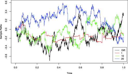
Figure 1: Plots of sample paths of $X$ of (20) for $\delta=1,10$ and $20$, with a diffusion corresponding to $X$ with $J$ replaced by a standard Wiener process.

2.4 A numerical example

For simulation purposes, we consider the following concrete model:

$$dX_{t}=\frac{-\alpha X_{t}}{\sqrt{1+X_{t}^{2}}}\,dt+\sqrt{\beta}\,dJ_{t},\qquad X_{0}=0,$$ (20)

where the true value is $(\alpha_{0},\beta_{0})=(1,1)$, the driving process is the normal inverse Gaussian Lévy process such that $\mathcal{L}(J_{t})=\operatorname{NIG}(\delta,0,\delta t,0)$, where $\delta=1,10$ or $20$. It holds that $E[J_{t}]=0$, $E[J_{1}^{2}]=t$, and $\mathcal{L}(J_{t})\to\mathcal{N}(0,t)$ in total variation as $\delta\to\infty$, and that $\nu(3)=0$ and $\nu(4)=3/\delta^{2}$. Model (20) is a normal-inverse Gaussian counterpart to the hyperbolic diffusion, for which $J$ is replaced by a standard Wiener process. For this $X$, we can verify all the assumptions; see Proposition 5.4 for the verification of the stability conditions.

We simulated $1000$ independent paths by Euler scheme with sufficiently fine step size to obtain $1000$ independent estimates $\hat{\theta}_{n}=(\hat{\alpha}_{n},\hat{\alpha}_{n})$, and then computed their empirical mean and standard deviations.

Figure 1 shows typical sample paths of $X$ for $\delta=1,10$, and $20$, with a diffusion corresponding to $X$ with $J$ replaced with a standard Wiener process, just for comparison.

Table 1 reports the results; just for comparison, we included the case of diffusion, where $J$ is a standard Wiener process. From the table, we can observe the following:

• the performance of $\hat{\alpha}_{n}$ are rather similar for all the three cases;

• the performance of $\hat{\beta}_{n}$ gets better for larger $\delta$, which can be expected from the fact that the asymptotic variance of $\hat{\beta}_{n}$ is a constant multiple of $\nu(4)=3\delta^{-2}$; we have $\mathbb{V}_{\beta\beta}\to 0$ as $\delta\to\infty$.

Table 1: Finite sample performance of $\hat{\theta}_{n}$ concerning the model (20); just for comparison, the case of diffusion is also included. In each case, the sample mean is given with the sample standard deviation in parenthesis

		Diffusion		$\bolds{\delta=1}$		$\bolds{\delta=10}$		$\bolds{\delta=20}$
$\bolds{T_{n}}$	$\bolds{h_{n}}$	$\bolds{\alpha}$	$\bolds{\beta}$	$\bolds{\alpha}$	$\bolds{\beta}$	$\bolds{\alpha}$	$\bolds{\beta}$	$\bolds{\alpha}$	$\bolds{\beta}$
10	0.05	1.16	0.96	1.15	0.98	1.18	0.97	1.18	0.96
		(0.63)	(0.10)	(0.62)	(0.58)	(0.65)	(0.11)	(0.65)	(0.10)
	0.01	1.19	0.99	1.17	0.97	1.21	0.99	1.19	0.99
		(0.67)	(0.04)	(0.64)	(0.48)	(0.66)	(0.07)	(0.68)	(0.05)
100	0.05	1.00	0.97	1.00	0.98	1.00	0.97	1.01	0.97
		(0.18)	(0.03)	(0.19)	(0.17)	(0.18)	(0.04)	(0.17)	(0.03)
	0.01	1.02	0.99	1.02	1.00	1.02	0.99	1.03	1.00
		(0.18)	(0.01)	(0.19)	(0.17)	(0.18)	(0.02)	(0.19)	(0.02)

3 Mighty convergence of a class of continuous random fields

In this section, we prove a fundamental result concerning the “single-norming” mighty convergence of a continuous statistical random fields associated with general vector-valued estimating functions; here, the “single-norming” means that the rates of convergence are the same for all the arguments of the corresponding estimator. Theorem 3.5 below will serve as a fundamental tool in the proof of Theorem 2.7; the content of this section can be read independently of the main body.

To proceed, we need some notation. Denote by $\{\mathcal{X}_{n},\mathcal{A}_{n},(P_{\theta})_{\theta\in\Theta}\}_{n\in\mathbb{N}}$ underlying statistical experiments, where $\Theta\subset\mathbb{R}^{p}$ is a bounded convex domain. Let $\theta_{0}\in\Theta$, and write $P_{0}=P_{\theta_{0}}$. Let $\mathbb{G}_{n}=(\mathbb{G}_{j,n})_{j=1}^{p}\dvtx\mathcal{X}_{n}\times\Theta\to\mathbb{R}^{p}$ be vector-valued random functions; as usual, we will simply write $\mathbb{G}_{n}(\theta)$, dropping the argument of $\mathcal{X}_{n}$. Our target “contrast” function is

$$\mathbb{M}_{n}(\theta):=-\frac{1}{T_{n}}\bigl{|}\mathbb{G}_{n}(\theta)\bigr{|}^{2},$$ (21)

where $(T_{n})$ is a nonrandom positive real sequence such that $T_{n}\to\infty$. The corresponding “$M$-estimator” is defined to be any measurable mapping $\hat{\theta}_{n}\dvtx\mathcal{X}_{n}\to\overline{\Theta}$ such that

$$\hat{\theta}_{n}\in\mathop{\operatorname{argmax}}_{\theta\in\overline{\Theta}}\mathbb{M}_{n}(\theta).$$

Due to the compactness of $\overline{\Theta}$ and the continuity of $\mathbb{M}_{n}$ imposed later on, we can always find such a $\hat{\theta}_{n}$. The estimate $\hat{\theta}_{n}$ can be any root of $\mathbb{G}_{n}(\theta)=0$ as soon as it exists.

Set $U_{n}(\theta_{0}):=\{u\in\mathbb{R}^{p}\dvtx\theta_{0}+T_{n}^{-1/2}u\in\Theta\}$ and define random fields $\mathbb{Z}_{n}\dvtx\break U_{n}(\theta_{0})\to(0,\infty)$ by

$$\mathbb{Z}_{n}(u)=\mathbb{Z}_{n}(u;\theta_{0}):=\exp\bigl{\{}\mathbb{M}_{n}\bigl{(}\theta_{0}+T_{n}^{-1/2}u\bigr{)}-\mathbb{M}_{n}(\theta_{0})\bigr{\}}.$$ (22)

Obviously, it holds that

$$\hat{u}_{n}:=\sqrt{T_{n}}(\hat{\theta}_{n}-\theta_{0})\in\mathop{\operatorname{argmax}}_{\theta\in\overline{\Theta}}\mathbb{Z}_{n}(\theta).$$

We consider the following two conditions for the random fields $\mathbb{Z}_{n}$.

• [Polynomial type Large Deviation Inequality (PLDI)]. For every $M>0$, we have

  $$\sup_{r>0}\Bigl{\{}r^{M}\sup_{n\in\mathbb{N}}P_{0}\Bigl{[}\sup_{|u|>r}\mathbb{Z}_{n}(u)\geq e^{-r}\Bigr{]}\Bigr{\}}<\infty.$$ (23)

• (Weak convergence on compact sets). There exists a random field $\mathbb{Z}_{0}(\cdot)=\mathbb{Z}_{0}(\cdot;\theta_{0})$ such that $\mathbb{Z}_{n}\to^{\mathcal{L}}\mathbb{Z}_{0}$ in $\mathcal{C}(\overline{B(R)})$ for each $R>0$, where $\overline{B(R)}:=\{u\in\mathbb{R}^{p};|u|\leq R\}$.

Under these conditions, the mode of convergence of $\mathbb{Z}_{n}(\cdot)$ is mighty enough to deduce that the maximum-point sequence $(\hat{u}_{n})_{n}$ is $L^{q}(P_{0})$-bounded for every $q>0$, which especially implies that $(\hat{u}_{n})_{n}$ is tight: indeed, if (23) is in force,

$$\sup_{n\in\mathbb{N}}P_{0}\bigl{[}|\hat{u}_{n}|>r\bigr{]} \leq \sup_{n\in\mathbb{N}}P_{0}\Bigl{[}\sup_{|u|>r}\mathbb{Z}_{n}(u)\geq\mathbb{Z}_{n}(0)\Bigr{]}$$

$$= \sup_{n\in\mathbb{N}}P_{0}\Bigl{[}\sup_{|u|>r}\mathbb{Z}_{n}(u)\geq 1\Bigr{]}\lesssim\frac{1}{r^{M}}$$

for every $r>0$, so that

$$\sup_{n\in\mathbb{N}}E_{0}\bigl{[}|\hat{u}_{n}|^{q}\bigr{]}=\int_{0}^{\infty}\sup_{n\in\mathbb{N}}P_{0}\bigl{[}|\hat{u}_{n}|>s^{1/q}\bigr{]}\,ds\lesssim 1+\int_{1}^{\infty}s^{-M/q}\,ds<\infty.$$

If $u\mapsto\mathbb{Z}_{0}(u)$ is a.s. maximized at a unique point $\hat{u}_{\infty}$, then it follows from the tightness of $(\hat{u}_{n})_{n\in\mathbb{N}}$ that $\hat{u}_{n}\to^{\mathcal{L}}\hat{u}_{\infty}$; let us remind the reader that the weak convergence on any compact set alone is not enough to deduce the weak convergence of $\hat{u}_{n}$, since $U_{n}(\theta_{0})\uparrow\mathbb{R}^{p}$ and we have no guarantee that $(\hat{u}_{n})$ is tight. Moreover, owing to the PLDI, the moment of $f(\hat{u}_{n})$ converges to that of $f(\hat{u}_{\infty})$ for every continuous function $f$ on $\mathbb{R}^{p}$ of at most polynomial growth. In our framework, $\log\mathbb{Z}_{0}$ admits a quadratic structure with a normally distributed linear term and a nonrandom positive definite quadratic term, so that $\hat{u}_{\infty}$ is asymptotically normally distributed.

We now introduce regularity conditions.

Assumption 3.1 ((Smoothness)).

The functions $\theta\mapsto\mathbb{G}_{n}(\theta)$ are continuously extended to the boundary of $\Theta$, and belong to $\mathcal{C}^{3}(\Theta)$, $P_{0}$-a.s.

Assumption 3.2 ((Bounded moments)).

For every $K>0$,

$$\sup_{n\in\mathbb{N}}E_{0}\biggl{[}\biggl{|}\frac{1}{\sqrt{T_{n}}}\mathbb{G}_{n}(\theta_{0})\biggr{|}^{K}\biggr{]}+\max_{k\in\{0,1,2,3\}}\sup_{n\in\mathbb{N}}E_{0}\biggl{[}\sup_{\theta\in\Theta}\biggl{|}\frac{1}{T_{n}}\partial_{\theta}^{k}\mathbb{G}_{n}(\theta)\biggr{|}^{K}\biggr{]}<\infty.$$

Let $M>0$ be a given constant.

Assumption 3.3 ((Limits)).

(a) There exist a nonrandom function $\mathbb{G}_{\infty}\dvtx\break\Theta\to\mathbb{R}^{p}$ and positive constants $\chi=\chi(\theta_{0})$ and $\varepsilon$ such that: $\mathbb{G}_{\infty}(\theta_{0})=0$; $\sup_{\theta}|\mathbb{G}_{\infty}(\theta)|<\infty$; $|\mathbb{G}_{\infty}(\theta)|^{2}\geq\chi|\theta-\theta_{0}|^{2}$ for every $\theta\in\Theta$; and

$$\sup_{n\in\mathbb{N}}E_{0}\biggl{[}\sup_{\theta\in\Theta}\biggl{|}\sqrt{T_{n}}\biggl{(}\frac{1}{T_{n}}\mathbb{G}_{n}(\theta)-\mathbb{G}_{\infty}(\theta)\biggr{)}\biggr{|}^{M+\varepsilon}\biggr{]}<\infty.$$

[(b)]

There exists a nonrandom $\mathbb{G}_{\infty}^{\prime}(\theta_{0})\in\mathbb{R}^{p}\otimes\mathbb{R}^{p}$ of rank $p$ such that

$$\sup_{n\in\mathbb{N}}E_{0}\biggl{[}\biggl{|}\sqrt{T_{n}}\biggl{(}\frac{1}{T_{n}}\partial_{\theta}\mathbb{G}_{n}(\theta_{0})-\mathbb{G}_{\infty}^{\prime}(\theta_{0})\biggr{)}\biggr{|}^{M}\biggr{]}<\infty.$$

Assumption 3.4 ((Weak convergence)).

$T_{n}^{-1/2}\mathbb{G}_{n}(\theta_{0})\to^{\mathcal{L}}\mathcal{N}_{p}(0,\mathbb{V}(\theta_{0}))$ for some positive definite $\mathbb{V}(\theta_{0})\in\mathbb{R}^{p}\otimes\mathbb{R}^{p}$.

Let $\Sigma(\theta_{0}):=(\mathbb{G}^{\prime}_{\infty})^{-1}\mathbb{V}(\mathbb{G}^{\prime}_{\infty})^{-1\top}(\theta_{0})$. The main claim of this section is the following.

Theorem 3.5

Let $M>0$. [(a)]

Suppose that Assumptions 3.1, 3.2 and 3.3 hold. Then the PLDI (23) holds true.

If Assumption 3.4 is additionally met, then

$$E_{0}\bigl{[}f(\hat{u}_{n})\bigr{]}\to\int f(u)\phi\bigl{(}u;0,\Sigma(\theta_{0})\bigr{)}\,du$$

for every continuous function $f\dvtx\mathbb{R}^{p}\to\mathbb{R}$ satisfying that $\limsup_{|u|\to\infty}|u|^{-q}\times|f(u)|<\infty$ for some $q\in(0,M)$.

Applying Taylor’s expansion to (22), we get

$$\log\mathbb{Z}_{n}(u)=\Delta_{n}(\theta_{0})[u]-\tfrac{1}{2}\Gamma(\theta_{0})[u,u]+\xi_{n}(u),$$ (24)

where $\Delta_{n}(\theta_{0}):=T_{n}^{-1/2}\,\partial_{\theta}\mathbb{M}_{n}(\theta_{0})$, $\Gamma_{n}(\theta_{0}):=-T_{n}^{-1}\,\partial_{\theta}^{2}\mathbb{M}_{n}(\theta_{0})$, $\Gamma(\theta_{0}):=\break 2\mathbb{G}^{\prime}_{\infty}(\theta_{0})^{\top}\mathbb{G}^{\prime}_{\infty}(\theta_{0})$ and

$$\xi_{n}(u) := \frac{1}{2}\bigl{\{}\Gamma(\theta_{0})-\Gamma_{n}(\theta_{0})\bigr{\}}[u,u]$$

$${}-\int_{0}^{1}(1-s)\int\partial_{\theta}\Gamma_{n}\bigl{(}\theta_{0}+stT_{n}^{-1/2}u\bigr{)}\bigl{[}sT_{n}^{-1/2}u,u^{\otimes 2}\bigr{]}\,dt\,ds.$$

We will prove (a) by making use of Yoshida Yos11 , Theorem 3(c). The task is then to verify conditions [A1^′′], [A4^′], [A6], [B1] and [B2] of that paper. For convenience and clarity, we will list them in a reduced form with our notation. First we look at [B1] and [B2]: [[B1]]

the matrix $\Gamma(\theta_{0})$ is positive definite;

there exists a constant $\chi>0$ such that $\mathbb{Y}(\theta)\leq-\chi^{2}|\theta-\theta_{0}|^{2}$ for each $\theta\in\Theta$. Here $\mathbb{Y}(\theta):=-|\mathbb{G}_{\infty}(\theta)|^{2}$, where $\mathbb{G}_{\infty}(\theta)$ is the one appearing in Assumption 3.3. Obviously, Assumption 3.3 assures [B1] and [B2] (the identifiability); in particular, we have the convergence $T_{n}^{-1}\mathbb{M}_{n}(\theta)\to^{p}-|\mathbb{G}_{\infty}(\theta)|^{2}$ for each $\theta\in\Theta$, so that

$$\mathbb{Y}_{n}(\theta):=\frac{1}{T_{n}}\bigl{\{}\mathbb{M}_{n}(\theta)-\mathbb{M}_{n}(\theta_{0})\bigr{\}}=\frac{1}{T_{n}}\log\mathbb{Z}_{n}\bigl{(}\sqrt{T_{n}}(\theta-\theta_{0})\bigr{)}\to^{p}\mathbb{Y}(\theta).$$

Next, given constants $M>0$ [the number in (23)] and $\alpha\in(0,1)$, conditions [A6], [A1^′′] and [A4^′] read as follows:

1. [[A4^′]]

2. (i)  $\sup_{n}E_{0}[|\Delta_{n}(\theta_{0})|^{M_{1}}]<\infty$ for $M_{1}:=M/(1-\rho_{1})$.

   1. [(ii)]

   2. $\sup_{n}E_{0}[\sup_{\theta}|T_{n}^{1/2-\beta_{2}}(\mathbb{Y}_{n}(\theta)-\mathbb{Y}(\theta))|^{M_{2}}]<\infty$, for $M_{2}:=M/(1-2\beta_{2}-\rho_{2})$.

3. 1. $\sup_{n}E_{0}[\sup_{\theta}|T_{n}^{-1}\partial_{\theta}^{3}\mathbb{M}_{n}(\theta)|^{M_{3}}]<\infty$ for $M_{3}:=M/\{\alpha/(1-\alpha)-\rho_{1}\}$.

   2. $\sup_{n}E_{0}[|T_{n}^{\beta_{1}}(\Gamma_{n}(\theta_{0})-\Gamma(\theta_{0})|^{M_{4}}]<\infty$ for $M_{4}:=M/\{2\beta_{1}/(1-\alpha)-\rho_{1}\}$.

4. The parameters $\alpha$, $\beta_{1}$, $\beta_{2}$, $\rho_{1}$ and $\rho_{2}$ fulfil the inequalities

   $$\displaystyle 0<\beta_{1}<1/2,\qquad 0<\rho_{1}<\min\biggl{(}1,\frac{\alpha}{1-\alpha},\frac{2\beta_{1}}{1-\alpha}\biggr{)},$$

   $$\displaystyle 2\alpha<\rho_{2},\qquad\beta_{2}\geq 0,\qquad 1-2\beta_{2}-\rho_{2}>0.$$

These conditions involve several “moment-index” parameters to be controlled, which do not seem straightforward to handle. Nevertheless, under our assumptions we can provide a rather simplified version. Instead of “[A1^′′], [A4^′] and [A6]” we will verify the following “[A1${}^{\prime\prime}{}^{\sharp}$] and [A6^♯]”:

1. [[A1${}^{\prime\prime}{}^{\sharp}$]]

2. (i)  $\sup_{n}E_{0}[\sup_{\theta}|T_{n}^{-1}\partial_{\theta}^{3}\mathbb{M}_{n}(\theta)|^{K}]<\infty$ for every $K>0$.

   1. [(ii)]

   2. $\sup_{n}E_{0}[|\sqrt{T_{n}}(\Gamma_{n}(\theta_{0})-\Gamma(\theta_{0})|^{M-\varepsilon_{1}}]<\infty$ for every $\varepsilon_{1}>0$ small enough.

3. (i)  $\sup_{n}E_{0}[|\Delta_{n}(\theta_{0})|^{K}]<\infty$ for every $K>0$.

   1. $\sup_{n}E_{0}[\sup_{\theta}|\sqrt{T_{n}}(\mathbb{Y}_{n}(\theta)-\mathbb{Y}(\theta))|^{M+\varepsilon/2}]<\infty$, for $\varepsilon$ given in Assumption 3.3.

Let us show that “[A1${}^{\prime\prime}{}^{\sharp}$] and [A6^♯]” imply “[A1^′′], [A4^′] and [A6].” First, by [A1${}^{\prime\prime}{}^{\sharp}$](i) and [A6^♯](i), the numbers $M_{1}$ and $M_{3}$ can be arbitrarily large, so that we may in particular take $\alpha$ and $\rho_{1}$ arbitrarily small (i.e., nearly zero). Then we have [A1^′′](i) and [A6](i). Next, we note that in [A1${}^{\prime\prime}{}^{\sharp}$](ii) the exponent of “$T_{n}$” is $1/2$, hence we may let $\beta_{2}$ be sufficiently close to $1/2$. Then, taking $\alpha$ and $\rho_{1}$ small enough with $\rho_{1}<\alpha/(1-\alpha)$, we can obtain the first two inequalities in [A4^′]. Next, in view of [A6^♯](ii), we can take $\beta_{2}=0$ and $\rho_{2}$ small enough to make [A6](ii) and the last three ones in [A4^′] valid. Finally, as for $M_{4}$, we note that a suitable control of $(\alpha,\rho_{1},\beta_{1})$ leads to

$$\frac{2\beta_{1}}{1-\alpha}-\rho_{1}=1+\biggl{(}\frac{\alpha}{1-\alpha}-\rho_{1}\biggr{)}+\frac{2\beta_{1}-1}{1-\alpha}>1,$$

so that [A1^′′](ii) follows. In sum, under “[A1${}^{\prime\prime}{}^{\sharp}$] and [A6^♯],” we can pick $\rho_{1},\rho_{2},\alpha\approx 0$ and $\beta_{2}=0$, and then $\beta_{1}\approx 1/2$, in order to make all of “[A1^′′], [A4^′] and [A6]” valid. Thus we are left to proving [A1${}^{\prime\prime}{}^{\sharp}$] and [A6^♯] above.

We begin with [A1${}^{\prime\prime}{}^{\sharp}$]. Since $|T_{n}^{-1}\partial_{\theta}^{3}\mathbb{M}_{n}(\theta)|\lesssim|T_{n}^{-1}\mathbb{G}_{n}(\theta)\|T_{n}^{-1}\partial_{\theta}^{3}\mathbb{G}_{n}(\theta)|+|T_{n}^{-1}\partial_{\theta}\mathbb{G}_{n}(\theta)\|T_{n}^{-1}\partial_{\theta}^{2}\mathbb{G}_{n}(\theta)|$, we have for every $K>0$,

$$\sup_{n\in\mathbb{N}}E_{0}\biggl{[}\sup_{\theta\in\Theta}\biggl{|}\frac{1}{T_{n}}\partial_{\theta}^{3}\mathbb{M}_{n}(\theta)\biggr{|}^{K}\biggr{]}<\infty.$$

Noting that $\partial_{\theta_{i}}\,\partial_{\theta_{j}}\mathbb{M}_{n}=-2T_{n}^{-1}\{\partial_{\theta_{i}}\,\partial_{\theta_{j}}\mathbb{G}_{n}[\mathbb{G}_{n}]+\partial_{\theta_{i}}\mathbb{G}_{n}[\partial_{\theta_{j}}\mathbb{G}_{n}]\}$, we also have

$$\sqrt{T_{n}}\bigl{|}\Gamma_{n}(\theta_{0})-\Gamma(\theta_{0})\bigr{|}$$

$$\qquad\lesssim\biggl{|}\frac{1}{\sqrt{T_{n}}}\mathbb{G}_{n}(\theta_{0})\biggr{|}\biggl{|}\frac{1}{T_{n}}\partial_{\theta}^{2}\mathbb{G}_{n}(\theta_{0})\biggr{|}$$

$$\qquad\quad{}{}+\biggl{(}\bigl{|}\Gamma(\theta_{0})\bigr{|}+\biggl{|}\frac{1}{T_{n}}\partial_{\theta}\mathbb{G}_{n}(\theta_{0})\biggr{|}\biggr{)}\biggl{|}\sqrt{T_{n}}\biggl{(}\frac{1}{T_{n}}\partial_{\theta}\mathbb{G}_{n}(\theta_{0})-\mathbb{G}^{\prime}_{\infty}(\theta_{0})\biggr{)}\biggr{|}.$$

Therefore, Assumptions 3.2 and 3.3 combined with Hölder’s inequality yield that for $\varepsilon_{1}\in(0,M)$,

$$\sup_{n\in\mathbb{N}}E_{0}\bigl{[}\bigl{|}\sqrt{T_{n}}(\Gamma_{n}(\theta_{0})-\Gamma(\theta_{0})\bigr{|}^{M-\varepsilon_{1}}\bigr{]}$$

$$\qquad\lesssim 1+\biggl{\{}\sup_{n\in\mathbb{N}}E_{0}\biggl{[}\biggl{|}\sqrt{T_{n}}\biggl{(}\frac{1}{T_{n}}\partial_{\theta}\mathbb{G}_{n}(\theta_{0})-\mathbb{G}^{\prime}_{\infty}(\theta_{0})\biggr{)}\biggr{|}^{M}\biggr{]}\biggr{\}}^{(M-\varepsilon_{1})/M}<\infty.$$

Thus [A1${}^{\prime\prime}{}^{\sharp}$] follows.

Next we prove [A6^♯]. Statement (i) is obvious from Assumption 3.2,

$$\quad\sup_{n\in\mathbb{N}}E_{0}\bigl{[}\bigl{|}\Delta_{n}(\theta_{0})\bigr{|}^{K}\bigr{]}\lesssim\sup_{n\in\mathbb{N}}E_{0}\biggl{[}\biggl{|}\frac{1}{T_{n}}\partial_{\theta}\mathbb{G}_{n}(\theta_{0})\biggr{|}^{K}\biggl{|}\frac{1}{\sqrt{T_{n}}}\mathbb{G}_{n}(\theta_{0})\biggr{|}^{K}\biggr{]}<\infty.$$ (26)

Using the estimate

$$\bigl{|}\sqrt{T_{n}}\bigl{(}\mathbb{Y}_{n}(\theta)-\mathbb{Y}(\theta)\bigr{)}\bigr{|}$$

$$\qquad\leq\frac{1}{\sqrt{T_{n}}}\biggl{|}\frac{1}{\sqrt{T_{n}}}\mathbb{G}_{n}(\theta_{0})\biggr{|}^{2}$$

$$\qquad\quad{}+\biggl{(}\bigl{|}\mathbb{G}_{\infty}(\theta)\bigr{|}+\biggl{|}\frac{1}{T_{n}}\mathbb{G}_{n}(\theta)\biggr{|}\biggr{)}\biggl{|}\sqrt{T_{n}}\biggl{(}\frac{1}{T_{n}}\mathbb{G}_{n}(\theta)-\mathbb{G}_{\infty}(\theta)\biggr{)}\biggr{|},$$

it follows under Assumptions 3.2 and 3.3 that

$$\sup_{n\in\mathbb{N}}E_{0}\Bigl{[}\sup_{\theta\in\Theta}\bigl{|}\sqrt{T_{n}}\bigl{(}\mathbb{Y}_{n}(\theta)-\mathbb{Y}(\theta)\bigr{)}\bigr{|}^{M+\varepsilon/2}\Bigr{]}$$

$$\quad\lesssim 1+\sup_{n\in\mathbb{N}}E_{0}\biggl{[}\sup_{\theta\in\Theta}\biggl{|}\sqrt{T_{n}}\biggl{(}\frac{1}{T_{n}}\mathbb{G}_{n}(\theta)-\mathbb{G}_{\infty}(\theta)\biggr{)}\biggr{|}^{M+\varepsilon}\biggr{]}^{(M+\varepsilon/2)/(M+\varepsilon)}<\infty.$$

Thus [A6^♯] is ensured, and the proof of (a) is complete.

We now turn to the proof of (b). Fix any $R>0$. Since we know that the sequence $(\hat{u}_{n})$ is $L^{q}(P_{0})$-bounded for each $q\in(0,M)$ and that the set $\mathop{\operatorname{argmax}}_{u}\log\mathbb{Z}_{\infty}(u)$ a.s. consists of the only point

$$\hat{u}_{\infty}:=\Gamma(\theta_{0})^{-1}\Delta_{\infty}(\theta_{0})\sim\mathcal{N}_{p}\bigl{(}0,\Sigma(\theta_{0})\bigr{)},$$

it suffices to show that $\log\mathbb{Z}_{n}\to^{\mathcal{L}}\log\mathbb{Z}_{\infty}$ in $\mathcal{C}(\overline{B(R)})$, where

$$\log\mathbb{Z}_{\infty}(u) := \Delta_{\infty}(\theta_{0})[u]-\tfrac{1}{2}\Gamma(\theta_{0})[u,u],$$

$$\Delta_{\infty}(\theta_{0}) \sim \mathcal{N}_{p}\bigl{(}0,4\mathbb{G}^{\prime}_{\infty}(\theta_{0})^{\top}\mathbb{V}(\theta_{0})\mathbb{G}^{\prime}_{\infty}(\theta_{0})\bigr{)}$$

(e.g., Yoshida Yos11 , Theorem 5). We have $T_{n}^{-1}\partial_{\theta}\mathbb{G}_{n}(\theta_{0})\to^{p}\mathbb{G}_{\infty}^{\prime}(\theta_{0})$ from Assumption 3.3, hence Slutsky’s lemma and Assumption 3.4 imply that

$$\Delta_{n}(\theta_{0})=-\frac{2}{T_{n}}\partial_{\theta}\mathbb{G}_{n}(\theta_{0})\biggl{[}\frac{1}{\sqrt{T_{n}}}\mathbb{G}_{n}(\theta_{0})\biggr{]}\to^{\mathcal{L}}\Delta_{\infty}(\theta_{0}).$$

Also, we have

$$\bigl{|}\xi_{n}(u)\bigr{|}\lesssim|u|^{2}\bigl{|}\Gamma_{n}(\theta_{0})-\Gamma(\theta_{0})\bigr{|}+\frac{|u|^{3}}{\sqrt{T_{n}}}\sup_{\theta\in\Theta}\biggl{|}\frac{1}{T_{n}}\partial_{\theta}^{3}\mathbb{M}_{n}(\theta)\biggr{|}=o_{p}(1)$$ (27)

for every $u\in\overline{B(R)}$. Thus, recalling expression (24), we get $\log\mathbb{Z}_{n}(u)\to^{\mathcal{L}}\log\mathbb{Z}_{0}(u)$ for every $u\in\overline{B(R)}$, and moreover, due to the linearity in $u$ of the weak convergence term $\Delta_{n}(\theta_{0})[u]$, the Cramér–Wold device ensures the finite-dimensional convergence. Therefore, it remains to check the tightness of $\{\log\mathbb{Z}_{n}(u)\}_{u\in\overline{B(R)}}$. In view of the classical Kolmogorov tightness criterion for continuous random fields (e.g., Kunita Kun90 , Theorem 1.4.7), it suffices to show that there exists a constant $\gamma>p(=\operatorname{dim}\Theta)$ such that

$$\sup_{|u|\leq R}\sup_{n\in\mathbb{N}}E_{0}\bigl{[}\bigl{|}\log\mathbb{Z}_{n}(u)\bigr{|}^{\gamma}\bigr{]}+\sup_{n\in\mathbb{N}}E_{0}\Bigl{[}\sup_{|u|\leq R}\bigl{|}\partial_{u}\log\mathbb{Z}_{n}(u)\bigr{|}^{\gamma}\Bigr{]}<\infty.$$ (28)

In view of the estimates in (26) and (27) as well as the expressions (24) and (3),

$$\sup_{u\in\overline{B(R)}}\sup_{n\in\mathbb{N}}E_{0}\bigl{[}\bigl{|}\log\mathbb{Z}_{n}(u)\bigr{|}^{\gamma}\bigr{]}$$

$$\qquad\lesssim\sup_{n\in\mathbb{N}}E_{0}\bigl{[}\bigl{|}\Delta_{n}(\theta_{0})\bigr{|}^{\gamma}\bigr{]}+1+\sup_{u\in\overline{B(R)}}\sup_{n\in\mathbb{N}}E_{0}\bigl{[}\bigl{|}\xi_{n}(u)\bigr{|}^{\gamma}\bigr{]}$$

$$\qquad\lesssim 1+E_{0}\bigl{[}\bigl{|}\Gamma_{n}(\theta_{0})-\Gamma(\theta_{0})\bigr{|}^{\gamma}\bigr{]}+\sup_{n\in\mathbb{N}}E_{0}\biggl{[}\sup_{\theta\in\Theta}\biggl{|}\frac{1}{T_{n}}\partial_{\theta}^{3}\mathbb{M}_{n}(\theta)\biggr{|}^{\gamma}\biggr{]}<\infty.$$

Furthermore, since

$$\partial_{u}\log\mathbb{Z}_{n}(u) = \partial_{u}\biggl{\{}\mathbb{M}_{n}\biggl{(}\theta_{0}+\frac{1}{\sqrt{T_{n}}}u\biggr{)}-\mathbb{M}_{n}(\theta_{0})\biggr{\}}$$

$$= \frac{1}{\sqrt{T_{n}}}\partial_{\theta}\mathbb{M}_{n}\biggl{(}\theta_{0}+\frac{1}{\sqrt{T_{n}}}u\biggr{)}$$

$$= \frac{1}{\sqrt{T_{n}}}\biggl{\{}\partial_{\theta}\mathbb{M}_{n}(\theta_{0})+\frac{1}{\sqrt{T_{n}}}\int_{0}^{1}\partial_{\theta}^{2}\mathbb{M}_{n}\biggl{(}\theta_{0}+\frac{s}{\sqrt{T_{n}}}u\biggr{)}[u]\,ds\biggr{\}},$$

the finiteness of $\sup_{n}E_{0}[\sup_{|u|\leq R}|\partial_{u}\log\mathbb{Z}_{n}(u)|^{\gamma}]$ follows on applying Assumption 3.2 to the estimate

$$\sup_{|u|\leq R}\bigl{|}\partial_{u}\log\mathbb{Z}_{n}(u)\bigr{|}$$

$$\qquad\lesssim\biggl{|}\frac{1}{\sqrt{T_{n}}}\mathbb{G}_{n}(\theta_{0})\biggr{|}\biggl{|}\frac{1}{T_{n}}\partial_{\theta}\mathbb{G}_{n}(\theta_{0})\biggr{|}+\sup_{\theta\in\Theta}\biggl{|}\frac{1}{T_{n}}\partial_{\theta}^{2}\mathbb{M}_{n}(\theta)\biggr{|}$$

$$\qquad\lesssim\biggl{|}\frac{1}{\sqrt{T_{n}}}\mathbb{G}_{n}(\theta_{0})\biggr{|}\biggl{|}\frac{1}{T_{n}}\partial_{\theta}\mathbb{G}_{n}(\theta_{0})\biggr{|}$$

$$\qquad\quad{}+\sup_{\theta\in\Theta}\biggl{\{}\biggl{|}\frac{1}{T_{n}}\mathbb{G}_{n}(\theta)\biggr{|}\biggl{|}\frac{1}{T_{n}}\partial_{\theta}^{2}\mathbb{G}_{n}(\theta)\biggr{|}+\biggl{|}\frac{1}{T_{n}}\partial_{\theta}\mathbb{G}_{n}(\theta)\biggr{|}^{2}\biggr{\}}.$$

Thus we have obtained (28), thereby achieving the proof of (b).

Remark 3.6.

We have confined ourselves to the “single-norming (i.e., scalar-$T_{n}$)” case for the squared quasi-score function. Nevertheless, as in the original formulation of Yoshida Yos11 , Theorem 1, it would be also possible to deal with “multi-norming” cases where elements of $\hat{\theta}_{n}$ possibly converge at different rates, that is, cases of a matrix norming instead of the scalar norming $\sqrt{T_{n}}$. This would require somewhat more complicated arguments, but we do not need such an extension in this paper.

4 Proofs of Theorem 2.7 and Corollary 2.8

4.1 Proof of Theorem 2.7

The proof of Theorem 2.7 is achieved by applying Theorem 3.5. When we have a reasonable estimating function $\theta\mapsto\mathbb{G}_{n}(\theta)$ with which an estimator of $\theta$ is defined by a random root of the estimating equation $\mathbb{G}_{n}(\theta)=0$, it may be unclear what is the “single” associated contrast function to be maximized or minimized; for example, it would be often the case when $\mathbb{G}_{n}$ is constructed via a kind of (conditional-) moment fittings. The setup (31) below provides a way of converting the situation from $Z$-estimation to $M$-estimation.

4.1.1 Introductory remarks

At first glance, it seems that, in order to investigate the asymptotic behavior of $\hat{\theta}_{n}$, we may proceed as in the case of diffusions, expanding the GQL $\mathbb{Q}_{n}$ of (12) and then investigating asymptotic behaviors of the derivatives $\partial_{\theta}^{k}\mathbb{Q}_{n}$; see Yoshida Yos11 , Section 6, for details. Following this route, however, leads to an inconvenience, essentially due to the fact that $(h_{n}^{-1/2}\Delta_{j}X)_{j\leq n}$ is not $L^{q}(P_{0})$-bounded for $q>2$. To see this more precisely, let us take a brief look at the simple one-dimensional Lévy process $X_{t}=\alpha t+\sqrt{\beta}J_{t}$, with $\theta=(\alpha,\beta)\in\mathbb{R}\times(0,\infty)$ and $\mathcal{L}(J_{1})$ admitting finite moments. In this case, $\mathbb{Q}_{n}(\theta)=-\sum_{j}\{(\log\beta)+(\beta h_{n})^{-1}(\Delta_{j}X-\alpha h_{n})^{2}\}$,

$$\partial_{\alpha}\mathbb{Q}_{n}(\theta) = \sum_{j=1}^{n}\frac{2}{\beta}(\Delta_{j}X-\alpha h_{n}),$$

$$\partial_{\beta}\mathbb{Q}_{n}(\theta) = \sum_{j=1}^{n}\frac{1}{\beta^{2}h_{n}}\bigl{\{}(\Delta_{j}X-\alpha h_{n})^{2}-\beta h_{n}\bigr{\}},$$

$$\partial_{\alpha}^{2}\mathbb{Q}_{n}(\theta) = \frac{-2T_{n}}{\beta},\qquad\partial_{\alpha}\,\partial_{\beta}\mathbb{Q}_{n}(\theta)=-\sum_{j=1}^{n}\frac{2}{\beta^{2}}(\Delta_{j}X-\alpha h_{n}),$$

$$\partial_{\beta}^{2}\mathbb{Q}_{n}(\theta) = -\sum_{j=1}^{n}\frac{2}{\beta^{3}h_{n}}\biggl{\{}(\Delta_{j}X-\alpha h_{n})^{2}-\frac{\beta h_{n}}{2}\biggr{\}}.$$

We can deduce the convergences

$$\frac{1}{T_{n}}\partial_{\alpha}^{2}\mathbb{Q}_{n}(\theta_{0}) \to^{p} -2\beta_{0}^{-1},\qquad\frac{1}{\sqrt{n}\sqrt{T_{n}}}\partial_{\alpha}\,\partial_{\beta}\mathbb{Q}_{n}(\theta_{0})\to^{p}0,$$

$$\frac{1}{n}\partial_{\beta}^{2}\mathbb{Q}_{n}(\theta_{0}) \to^{p} -\beta_{0}^{-2},$$

so that the normalized quasi observed-information matrix$-D_{n}^{-1}\partial_{\theta}^{2}\mathbb{Q}_{n}(\theta_{0})D_{n}^{-1}\to^{p}\operatorname{diag}(2\beta_{0}^{-1},\beta_{0}^{-2})$, where $D_{n}:=\operatorname{diag}(\sqrt{T_{n}},\sqrt{n})$. In view of the classical Cramér-type method for $M$-estimation, we should then have a central limit theorem for the normalized quasi-score $\{T_{n}^{-1/2}\partial_{\alpha}\mathbb{Q}_{n}(\theta_{0}),\break n^{-1/2}\partial_{\beta}\mathbb{Q}_{n}(\theta_{0})\}$ for an asymptotic normality at rate $D_{n}$ to be valid for the $M$-estimator associated with $\mathbb{Q}_{n}$. However, different from the drifted Wiener process, the sequence $\{n^{-1/2}\partial_{\beta}\mathbb{Q}_{n}(\theta_{0})\}$ does not converge because $(h_{n}^{-1/2}\Delta_{j}X)_{j\leq n}$ cannot be $L^{q}$-bounded for large $q>2$ as can be seen from the moment structure of Lévy processes; see Luschgy and Pagès LusPag08 for general moment estimates in small time with several concrete examples. Although we only mentioned the Lévy process with diagonal norming, the situation remains the same even when $X$ is actually an ergodic solution to (1).

The observation made in the last paragraph says that the situation is different from the case of diffusions, when developing asymptotic theory concerning the Gaussian quasi-likelihood for model (1) under high-frequency sampling framework; it is also different from the case of time series models, where the usual $\sqrt{n}$-consistency holds in most cases (see the references cited in the Introduction). Earlier attempts to tackle this point have been made by Mancini Man04 , Shimizu and Yoshida ShiYos06 , Ogihara and Yoshida OgiYos11 , where they incorporated jump-detection filters in defining a contrast function. The filter approach has its own advantage such as $\sqrt{n}$-rate estimation of the diffusion parameter, even in the presence of jumps; however, we should have in mind that its implementation involves fine-tuning parameters, thereby possibly preventing us from a straightforward use of the approach.

In order to prove Theorem 2.7, we will look at not $\theta\mapsto\mathbb{Q}_{n}(\theta)$, but

$$\theta\mapsto\mathbb{G}_{n}(\theta)=\bigl{\{}\mathbb{G}^{\alpha}_{n}(\theta),\mathbb{G}^{\beta}_{n}(\theta)\bigr{\}},$$

where $\mathbb{G}^{\alpha}_{n}\dvtx\Theta\to\mathbb{R}^{p_{\alpha}}$ and $\mathbb{G}^{\beta}_{n}\dvtx\Theta\to\mathbb{R}^{p_{\beta}}$ are defined by

$$\mathbb{G}^{\alpha}_{n}(\theta) = \sum_{j=1}^{n}\partial_{\alpha}a_{j-1}(\alpha)\bigl{[}V_{j-1}^{-1}(\beta)\bigl{[}\chi_{j}(\alpha)\bigr{]}\bigr{]},$$ (29)

$$\mathbb{G}^{\beta}_{n}(\theta) = \sum_{j=1}^{n}\biggl{(}\bigl{\{}-\partial_{\beta}V_{j-1}^{-1}(\beta)\bigr{\}}\bigl{[}\chi_{j}(\alpha)^{\otimes 2}\bigr{]}-h_{n}\frac{\partial_{\beta}|V_{j-1}(\beta)|}{|V_{j-1}(\beta)|}\biggr{)}.$$ (30)

Our contrast function $\mathbb{M}_{n}(\theta)$ is then defined to be the “squared quasi-score” as in (21),

$$\mathbb{M}_{n}(\theta)=-\frac{1}{T_{n}}\bigl{|}\mathbb{G}_{n}(\theta)\bigr{|}^{2}.$$ (31)

Trivially, $\mathbb{G}_{n}\dvtx\Theta\to\mathbb{R}^{p}$ fulfil that $\mathbb{G}_{n}(\theta)=\{(1/2)\partial_{\alpha}\mathbb{Q}_{n}(\theta),h_{n}\,\partial_{\beta}\mathbb{Q}_{n}(\theta)\}$. The difference is that we put the factor “$h_{n}$” in front of $\partial_{\beta}\mathbb{Q}_{n}(\theta)$; our estimating procedure is formally not the usual $M$-estimation based on the Taylor expansion of $\theta\mapsto\mathbb{Q}_{n}(\theta)$ around $\theta_{0}$, but rather a kind of minimum distance estimation concerning the Gaussian quasi-score function. The optimization with respect to $\theta$ is asymptotically the same for both of $\mathbb{Q}_{n}$ and $\mathbb{M}_{n}$: if there is no root $\theta\in\Theta$ for $\mathbb{G}_{n}(\theta)=0$, then we may assign any value (e.g., any element of $\Theta$) to $\hat{\theta}_{n}$, upholding the claim of Theorem 2.7.

Remark 4.1.

More general cases than (29) and (30) can be treated, such as

$$\mathbb{G}^{\alpha}_{n}(\theta) = \sum_{j=1}^{n}\bar{W}^{\alpha}_{j-1}(\theta)\bigl{\{}X_{t_{j}}-m_{j-1}(\theta)\bigr{\}},$$

$$\mathbb{G}^{\beta}_{n}(\theta) = \sum_{j=1}^{n}\bigl{(}\bar{W}^{\beta,1}_{j-1}(\theta)\bigl{[}\bigl{\{}X_{t_{j}}-m_{j-1}(\theta)\bigr{\}}^{\otimes 2}\bigr{]}-h_{n}\bar{W}^{\beta,2}_{j-1}(\theta)\bigr{)}$$

for some measurable $m\dvtx\mathbb{R}^{d}\times\Theta\to\mathbb{R}^{d}$, $\bar{W}^{\alpha}\dvtx\mathbb{R}^{d}\times\Theta\to\mathbb{R}^{p_{\alpha}}\otimes\mathbb{R}^{d}$, $\bar{W}^{\beta,1}\dvtx\mathbb{R}^{d}\times\Theta\to\mathbb{R}^{p_{\beta}}\otimes(\mathbb{R}^{d}\otimes\mathbb{R}^{d})$ and $\bar{W}^{\beta,2}\dvtx\mathbb{R}^{d}\times\Theta\to\mathbb{R}^{p_{\beta}}$. This may be called a GQMLE as well, for we are still solely fitting the local mean vectors and covariance matrices. This setting allows us to deal with, for example, the parametric model

$$dX_{t}=a(X_{t},\theta)\,dt+b(X_{t},\theta)\,dW_{t}+c(X_{t-},\theta)\,dJ_{t}$$

with possibly degenerate $b$ and $c$, the resulting GQMLE $\hat{\theta}_{n}$ still being asymptotically normal at rate $\sqrt{T_{n}}$ under suitable conditions. To avoid unnecessarily messy notation and regularity conditions without losing essence, we have decided to treat (1) in this paper.

For later use, we here introduce some convention and recall a couple of basic facts that we will make use often without notice:

• We will often suppress “$(\theta_{0})$” from the notation: $\chi_{j}:=\chi_{j}(\alpha_{0})$, $a_{j-1}:=a_{j-1}(\alpha_{0})$, $\mathbb{G}_{n}^{\alpha}=\mathbb{G}_{n}^{\alpha}(\theta_{0})$, and so forth.

• $\int_{j}$ denotes a shorthand for $\int_{t_{j-1}}^{t_{j}}$.

• $M^{\prime}_{j-1}(\theta):=\partial_{\alpha}a_{j-1}(\alpha)^{\top}V_{j-1}^{-1}(\beta)\in\mathbb{R}^{p_{\alpha}}\otimes\mathbb{R}^{d}$.

• $M^{\prime\prime}_{j-1}(\beta):=-\partial_{\beta}V_{j-1}^{-1}(\beta)=\{V_{j-1}^{-1}(\partial_{\beta}V_{j-1})V_{j-1}^{-1}\}(\beta)\in\mathbb{R}^{p_{\beta}}\otimes\mathbb{R}^{d}\otimes\mathbb{R}^{d}$.

• $d_{j-1}(\beta):=|V_{j-1}(\beta)|^{-1}\partial_{\beta}|V_{j-1}(\beta)|\in\mathbb{R}^{p_{\beta}}$.

• Given real sequence $a_{n}$ and random variables $Y_{n}$ possibly depending on $\theta$, we write $Y_{n}=O^{\ast}_{p}(a_{n})$ if $\sup_{n,\theta}E_{0}[|a_{n}^{-1}Y_{n}|^{K}]<\infty$ for every $K>0$.

• $E_{0}^{j-1}[\cdot]:=E_{0}[\cdot|\mathcal{F}_{t_{j-1}}]$.

• $R$ denotes a generic function on $\mathbb{R}^{d}$, possibly depending on $n$ and $\theta$, for which there exists a constant $C\geq 0$ such that $\sup_{n,\theta}|R(x)|\leq C(1+|x|)^{C}$ for every $x\in\mathbb{R}^{d}$.

• Burkholder’s inequality: for a martingale difference array $(\zeta_{nj})_{j\leq n}$ and every $q\geq 2$,

  $$E_{0}\biggl{[}\max_{k\leq n}\biggl{|}\sum_{j\leq k}\frac{1}{\sqrt{n}}\zeta_{nj}\biggr{|}^{q}\biggr{]}\lesssim E_{0}\biggl{[}\biggl{(}\frac{1}{n}\sum_{j\leq n}\zeta_{nj}^{2}\biggr{)}^{q/2}\biggr{]}\lesssim\frac{1}{n}\sum_{i\leq n}E\bigl{[}|\zeta_{nj}|^{q}\bigr{]}.$$

  Moreover, if $b_{\cdot}$ and $c_{\cdot}$ are sufficiently integrable adapted processes, then

  $$E_{0}\biggl{[}\biggl{|}\int_{0}^{T}b_{s-}\,dW_{s}\biggr{|}^{q}\biggr{]} \lesssim T^{q/2-1}\int_{0}^{T}E_{0}\bigl{[}|b_{s}|^{q}\bigr{]}\,ds,$$

  $$E_{0}\biggl{[}\biggl{|}\int_{0}^{T}c_{s-}\,dJ_{s}\biggr{|}^{q}\biggr{]} \lesssim (1\vee T)^{q/2-1}\int_{0}^{T}E_{0}\bigl{[}|c_{s}|^{q}\bigr{]}\,ds$$

  for every $T>0$ and $q\geq 2$ such that $E[|J_{1}|^{q}]<\infty$.

• Sobolev’s inequality (e.g., Friedman Fri06 , Section 10.2),

  $$E_{0}\Bigl{[}\sup_{\theta\in\Theta}\bigl{|}u(\theta)\bigr{|}^{q}\Bigr{]}\lesssim\sup_{\theta\in\Theta}\bigl{\{}E_{0}\bigl{[}\bigl{|}u(\theta)\bigr{|}^{q}\bigr{]}+E_{0}\bigl{[}\bigl{|}\partial_{\theta}u(\theta)\bigr{|}^{q}\bigr{]}\bigr{\}}$$

  for $q>p$ and a random field $u\in\mathcal{C}^{1}(\Theta)$; recall that $p$ denotes the dimension of $\theta$ and that we are presupposing the boundedness and convexity of $\Theta$. We will make use of this type of inequality to derive some uniform-in-$\theta$ moment estimates for martingale terms.

We now turn to the proof of Theorem 2.7 by verifying the conditions of Theorem 3.5.

4.1.2 Verification of the conditions on $\mathbb{G}_{n}$

We rewrite $\mathbb{G}_{n}$ as follows:

$$\mathbb{G}^{\alpha}_{n}(\theta) = \sum_{j=1}^{n}M^{\prime}_{j-1}(\theta)[\chi_{j}]-h_{n}\sum_{j=1}^{n}M^{\prime}_{j-1}(\theta)\bigl{[}a_{j-1}(\alpha)-a_{j-1}\bigr{]},$$ (32)

$$\mathbb{G}^{\beta}_{n}(\theta) = \sum_{j=1}^{n}\bigl{\{}M^{\prime\prime}_{j-1}(\beta)\bigl{[}\chi_{j}^{\otimes 2}\bigr{]}-h_{n}\,d_{j-1}(\beta)\bigr{\}}$$

$${}+2h_{n}\sum_{j=1}^{n}M^{\prime\prime}_{j-1}(\beta)\bigl{[}\chi_{j},a_{j-1}-a_{j-1}(\alpha)\bigr{]}$$

$${}+h_{n}^{2}\sum_{j=1}^{n}M^{\prime\prime}_{j-1}(\beta)\bigl{[}\bigl{\{}a_{j-1}-a_{j-1}(\alpha)\bigr{\}}^{\otimes 2}\bigr{]}.$$

We have

$$\chi_{j}=\zeta_{j}+r_{j},$$ (34)

where

$$\zeta_{j} := \int_{j}\tilde{a}_{j-1}(s)\,ds+\int_{j}b(X_{s},\beta_{0})\,dW_{s}+\int_{j}c(X_{s-},\beta_{0})\,dJ_{s},$$ (35)

$$r_{j} := \int_{j}\bigl{\{}E_{0}^{j-1}\bigl{[}a(X_{s},\alpha_{0})\bigr{]}-a_{j-1}\bigr{\}}\,ds,$$ (36)

with $\tilde{a}_{j-1}(s):=a(X_{s},\alpha_{0})-E_{0}^{j-1}[a(X_{s},\alpha_{0})]$. Obviously, $(\zeta_{j})_{j\leq n}$ forms a martingale difference array with respect to the discrete-time filtration $(\mathcal{F}_{t_{j}})_{j\leq n}$.

Itô’s formula and the present integrability condition lead to

$$E_{0}^{j-1}\bigl{[}a(X_{s},\alpha_{0})\bigr{]}-a_{j-1}=\int_{j}E_{0}^{j-1}\bigl{[}\mathcal{A}a(X_{u},\alpha_{0})\bigr{]}\,du=h_{n}R_{j-1},$$ (37)

where $\mathcal{A}$ denotes the (extended) generator associated with $X$ under $P_{0}$, that is, for $f\in\mathcal{C}^{2}(\mathbb{R}^{d})$

$$\mathcal{A}f(x) = \partial f(x)\bigl{[}a(x,\alpha_{0})\bigr{]}+\frac{1}{2}\partial^{2}f(x)\bigl{[}b(x,\beta_{0})^{\otimes 2}\bigr{]}$$

$${}+\int\bigl{\{}f\bigl{(}x+c(x,\beta_{0})z\bigr{)}-f(x)-\partial f(x)\bigl{[}c(x,\beta_{0})z\bigr{]}\bigr{\}}\nu(dz).$$

Putting (36) and (37) together gives $r_{j}=h_{n}^{2}R_{j-1}$, therefore

$$\chi_{j}=\zeta_{j}+h_{n}^{2}R_{j-1}.$$ (38)

Assumption 3.1 obviously holds under the present differentiability conditions. We begin with verifying Assumption 3.2.

Lemma 4.2

For every $K>0$, we have

$$\sup_{n\in\mathbb{N}}E_{0}\biggl{[}\biggl{|}\frac{1}{\sqrt{T_{n}}}\mathbb{G}_{n}(\theta_{0})\biggr{|}^{K}\biggr{]}+\sup_{n\in\mathbb{N}}E_{0}\biggl{[}\sup_{\theta\in\Theta}\biggl{|}\frac{1}{T_{n}}\mathbb{G}_{n}(\theta)\biggr{|}^{K}\biggr{]}<\infty.$$

By substituting (38) in (32) and (4.1.2) and then rearranging the resulting terms, we have

$$\mathbb{G}_{n}^{\alpha}(\theta) = \sum_{j=1}^{n}M^{\prime}_{j-1}(\theta)\zeta_{j}+h_{n}\sum_{j=1}^{n}M^{\prime}_{j-1}(\theta)\bigl{\{}a_{j-1}-a_{j-1}(\alpha)\bigr{\}}$$

$${}+h_{n}^{2}\sum_{j=1}^{n}M^{\prime}_{j-1}(\theta)R_{j-1},$$

$$\mathbb{G}^{\beta}_{n}(\theta) = \sum_{j=1}^{n}\bigl{\{}M^{\prime\prime}_{j-1}(\beta)\bigl{[}\zeta_{j}^{\otimes 2}\bigr{]}-h_{n}d_{j-1}(\beta)\bigr{\}}$$

$${}+2h_{n}\sum_{j=1}^{n}M^{\prime\prime}_{j-1}(\beta)\bigl{[}\zeta_{j},a_{j-1}-a_{j-1}(\alpha)\bigr{]}+h_{n}^{2}\sum_{j=1}^{n}R_{j-1}.$$

To achieve the proof, we will separately look at $T_{n}^{-1/2}\mathbb{G}^{\alpha}_{n}$, $T_{n}^{-1/2}\mathbb{G}^{\beta}_{n}$, $T_{n}^{-1}\mathbb{G}^{\alpha}_{n}(\theta)$ and $T_{n}^{-1}\mathbb{G}^{\beta}_{n}(\theta)$. Fix any integer $K>(2\vee p)$ in the sequel.

First we prove $T_{n}^{-1/2}\mathbb{G}^{\alpha}_{n}=O^{\ast}_{p}(1)$. Observe that

$$\frac{1}{\sqrt{T_{n}}}\mathbb{G}^{\alpha}_{n} = \sum_{j=1}^{n}\frac{1}{\sqrt{T_{n}}}M^{\prime}_{j-1}\zeta_{j}+\sqrt{T_{n}h_{n}^{2}}\frac{1}{n}\sum_{j=1}^{n}M^{\prime}_{j-1}R_{j-1}$$

$$= \sum_{j=1}^{n}\frac{1}{\sqrt{T_{n}}}M^{\prime}_{j-1}\zeta_{j}+O^{\ast}_{p}\Bigl{(}\sqrt{T_{n}h_{n}^{2}}\Bigr{)}.$$

By (35),

$$\sum_{j=1}^{n}\frac{1}{\sqrt{T_{n}}}M^{\prime}_{j-1}\zeta_{j} = \sum_{j=1}^{n}\frac{1}{\sqrt{n}}\biggl{(}M^{\prime}_{j-1}\frac{1}{\sqrt{h_{n}}}\int_{j}b(X_{s},\beta_{0})\,dW_{s}\biggr{)}$$

$${}+\sqrt{h_{n}}\sum_{j=1}^{n}\frac{1}{\sqrt{n}}\biggl{(}M^{\prime}_{j-1}\frac{1}{h_{n}}\int_{j}\tilde{a}_{j-1}(s)\,ds\biggr{)}$$

$${}+\sum_{j=1}^{n}\frac{1}{\sqrt{T_{n}}}M^{\prime}_{j-1}\int_{j}c(X_{s-},\beta_{0})\,dJ_{s}.$$

Burkholder’s inequality implies that the first and second term on the right-hand side are $O^{\ast}_{p}(1)$ and $O^{\ast}_{p}(\sqrt{h_{n}})$, respectively. As for the last term, by writing $\mathbf{1}_{j}\dvtx(0,\infty)\to\{0,1\}$ for the identity function of the interval $(t_{j-1},t_{j}]$,

$$E_{0}\Biggl{[}\Biggl{|}\sum_{j=1}^{n}\frac{1}{\sqrt{T_{n}}}M^{\prime}_{j-1}\int_{j}c(X_{s-},\beta_{0})\,dJ_{s}\Biggr{|}^{K}\Biggr{]}$$

$$\qquad\lesssim T_{n}^{-K/2}E_{0}\Biggl{[}\Biggl{|}\int_{0}^{T_{n}}\sum_{j=1}^{n}\mathbf{1}_{j}(s)M^{\prime}_{j-1}c(X_{s-},\beta_{0})\,dJ_{s}\Biggr{|}^{K}\Biggr{]}$$

$$\qquad\lesssim T_{n}^{-K/2}T_{n}^{K/2-1}\int_{0}^{T_{n}}E_{0}\Biggl{[}\Biggl{(}\sum_{j=1}^{n}\mathbf{1}_{j}(s)\bigl{|}M^{\prime}_{j-1}c(X_{s-},\beta_{0})\bigr{|}\Biggr{)}^{K}\Biggr{]}\,ds$$ (42)

$$\qquad=\frac{1}{T_{n}}\int_{0}^{T_{n}}\sum_{j=1}^{n}\mathbf{1}_{j}(s)E_{0}\bigl{[}\bigl{|}M^{\prime}_{j-1}c(X_{s-},\beta_{0})\bigr{|}^{K}\bigr{]}\,ds$$

$$\qquad\lesssim\frac{1}{T_{n}}\sum_{j=1}^{n}\int_{j}\,ds=1,$$

and hence we are done.

We now prove $T_{n}^{-1/2}\mathbb{G}^{\beta}_{n}=O^{\ast}_{p}(1)$. In the sequel, we may and do suppose that $d=p_{\beta}=r^{\prime}=r^{\prime\prime}=1$: this reduction is possible because of the polarization identity

$$\bigl{[}S^{\prime},S^{\prime\prime}\bigr{]}=\frac{1}{4}\bigl{(}\bigl{[}S^{\prime}+S^{\prime\prime}\bigr{]}-\bigl{[}S^{\prime}-S^{\prime\prime}\bigr{]}\bigr{)},$$

which is valid for any two semimartingales $S^{\prime}$ and $S^{\prime\prime}$. By (38) and (4.1.2),

$$\frac{1}{\sqrt{T_{n}}}\mathbb{G}^{\beta}_{n}=\sum_{j=1}^{n}\frac{1}{\sqrt{T_{n}}}\bigl{(}M^{\prime\prime}_{j-1}\zeta_{j}^{2}-h_{n}d_{j-1}\bigr{)}+O^{\ast}_{p}\Bigl{(}\sqrt{T_{n}h_{n}^{2}}\Bigr{)},$$

so that it remains to verify

$$\sum_{j=1}^{n}\frac{1}{\sqrt{T_{n}}}M^{\prime\prime}_{j-1}\bigl{(}\zeta_{j}^{2}-h_{n}V_{j-1}\bigr{)}=O^{\ast}_{p}(1).$$ (43)

Define $\zeta_{j}(t)$ for $t\in(t_{j-1},t_{j}]$ by

$$\zeta_{j}(t) = \int_{t_{j-1}}^{t}\tilde{a}_{j-1}(s)\,ds+\int_{t_{j-1}}^{t}b(X_{s},\beta_{0})\,dW_{s}$$

$${}+\int_{t_{j-1}}^{t}c(X_{s-},\beta_{0})\,dJ_{s}.$$

Let $N(ds,dz)$ denote the Poisson random measure associated with $J$, and $\tilde{N}$ its compensated version [i.e., $J_{t}=\int_{0}^{t}\int z\tilde{N}(ds,dz)$]. The quadratic variation at time $t$ is then given as follows (cf. Jacod and Shiryaev JacShi03 , I.4.49(d), I.4.55(b)):

$$\bigl{[}\zeta_{j}(\cdot)\bigr{]}_{t} = \int_{t_{j-1}}^{t}b^{2}(X_{s-},\beta_{0})\,ds+\int_{t_{j-1}}^{t}\int c^{2}(X_{s-},\beta_{0})z^{2}N(ds,dz)$$

$$= (t-t_{j-1})V_{j-1}+\int_{t_{j-1}}^{t}\int c^{2}(X_{s-},\beta_{0})\tilde{N}(ds,dz)+\int_{t_{j-1}}^{t}g_{j-1}(s)\,ds,$$

where we used the assumption $\int z^{2}\nu(dz)=1$ (with the temporary assumption $r^{\prime\prime}=1$) and $g_{j-1}(s):=b^{2}(X_{s},\beta_{0})-b_{j-1}^{2}+c^{2}(X_{s-},\beta_{0})-c_{j-1}^{2}$. Applying the integration-by-parts formula, we get

$$\zeta_{j}^{2}-h_{n}V_{j-1} = \biggl{\{}2\int_{j}\zeta_{j}(s-)\,d\zeta_{j}(s)+\int_{j}\int c^{2}(X_{s-},\beta_{0})z^{2}\tilde{N}(ds,dz)$$

$$\hskip 72.0pt{}+\int_{j}\bigl{(}g_{j-1}(s)-E_{0}^{j-1}\bigl{[}g_{j-1}(s)\bigr{]}\bigr{)}\,ds\biggr{\}}$$

$${}+\int_{j}E_{0}^{j-1}\bigl{[}g_{j-1}(s)\bigr{]}\,ds$$

$$=: \zeta^{(0)}_{j}+\zeta^{(1)}_{j}\qquad\mbox{say.}$$

We can deduce that $\sum_{j=1}^{n}T_{n}^{-1/2}M^{\prime\prime}_{j-1}\zeta^{(0)}_{j}=O^{\ast}_{p}(1)$, as is the case in the proof of $\sum_{j=1}^{n}T_{n}^{-1/2}M^{\prime}_{j-1}\zeta_{j}=O^{\ast}_{p}(1)$ via the expression (4.1.2). Moreover, we can apply Itô’s formula to get $\zeta^{(1)}_{j}=h_{n}^{2}R_{j-1}$ under the $\mathcal{C}^{2}$ property of $x\mapsto(b(x,\beta_{0}),c(x,\beta_{0}))$, from which it follows that $\sup_{n}E_{0}[|\sum_{j=1}^{n}T_{n}^{-1/2}M^{\prime\prime}_{j-1}\times\zeta^{(1)}_{j}|^{K}]\lesssim\sup_{n}(T_{n}h_{n}^{2})^{K/2}<\infty$. We thus get (43).

Let us turn to prove $\sup_{\theta}|T_{n}^{-1}\mathbb{G}^{\alpha}_{n}(\theta)|=O^{\ast}_{p}(1)$. In the same way as in the proof of $T_{n}^{-1/2}\mathbb{G}^{\alpha}_{n}=O^{\ast}_{p}(1)$, we can prove $\sum_{j=1}^{n}T_{n}^{-1/2}M^{\prime}_{j-1}(\theta)\zeta_{j}=O^{\ast}_{p}(T_{n}^{-1/2})$ for each $\theta\in\Theta$, since the explicit dependence on $\theta$ is only through the predictable parts $M^{\prime}_{j-1}(\theta)$; similar arguments will apply in some places below. Therefore, it follows from (4.1.2) that, for each $\theta\in\Theta$,

$$\frac{1}{T_{n}}\mathbb{G}_{n}^{\alpha}(\theta) = \frac{1}{\sqrt{T_{n}}}\Biggl{(}\sum_{j=1}^{n}\frac{1}{\sqrt{T_{n}}}M^{\prime}_{j-1}(\theta)\zeta_{j}\Biggr{)}+h_{n}\Biggl{(}\frac{1}{n}\sum_{j=1}^{n}M^{\prime}_{j-1}(\theta)R_{j-1}\Biggr{)}$$

$${}+\frac{1}{n}\sum_{j=1}^{n}M^{\prime}_{j-1}(\theta)\bigl{\{}a_{j-1}-a_{j-1}(\alpha)\bigr{\}}$$

$$= O_{p}^{\ast}\biggl{(}\frac{1}{\sqrt{T_{n}}}\vee h_{n}\biggr{)}+\frac{1}{n}\sum_{j=1}^{n}M^{\prime}_{j-1}(\theta)\bigl{\{}a_{j-1}-a_{j-1}(\alpha)\bigr{\}}$$

$$= O_{p}^{\ast}\biggl{(}\frac{1}{\sqrt{T_{n}}}\biggr{)}+\frac{1}{n}\sum_{j=1}^{n}M^{\prime}_{j-1}(\theta)\bigl{\{}a_{j-1}-a_{j-1}(\alpha)\bigr{\}},$$

so that $T_{n}^{-1}\mathbb{G}_{n}^{\alpha}(\theta)=O^{\ast}_{p}(1)$. In a quite similar manner, we obtain [see (4.1.3) and (4.1.3) below]

$$\frac{1}{T_{n}}\partial_{\theta}\mathbb{G}_{n}^{\alpha}(\theta)$$

$$\qquad=O_{p}^{\ast}\biggl{(}\frac{1}{\sqrt{T_{n}}}\biggr{)}+\frac{1}{n}\sum_{j=1}^{n}\partial_{\theta}\bigl{[}M^{\prime}_{j-1}(\theta)\bigl{\{}a_{j-1}-a_{j-1}(\alpha)\bigr{\}}\bigr{]}=O^{\ast}_{p}(1).$$

Therefore, we arrive at $\sup_{\theta}|T_{n}^{-1}\mathbb{G}^{\alpha}_{n}(\theta)|=O^{\ast}_{p}(1)$ by means of the Sobolev inequality.

It remains to prove $\sup_{\theta}|T_{n}^{-1}\mathbb{G}^{\beta}_{n}(\theta)|=O^{\ast}_{p}(1)$; we remind the reader that we are supposing that $d=p_{\beta}=r^{\prime}=r^{\prime\prime}=1$. As in the proof of (43), we can prove

$$\sum_{j=1}^{n}\frac{1}{\sqrt{T_{n}}}\partial_{\theta}^{k}M^{\prime\prime}_{j-1}(\beta)\bigl{(}\zeta_{j}^{2}-h_{n}V_{j-1}\bigr{)}=O^{\ast}_{p}(1)$$

for each $k=0,1$ and $\beta$, so that the Sobolev inequality gives $\sum_{j=1}^{n}T_{n}^{-1/2}\times M^{\prime\prime}_{j-1}(\beta)(\zeta_{j}^{2}-h_{n}V_{j-1})=O^{\ast}_{p}(1)$. Therefore, it follows from (4.1.2) and simple manipulation that

$$\frac{1}{T_{n}}\mathbb{G}^{\beta}_{n}(\theta) = \frac{1}{\sqrt{T_{n}}}\Biggl{(}\sum_{j=1}^{n}\frac{1}{\sqrt{T_{n}}}M^{\prime\prime}_{j-1}(\beta)\bigl{(}\zeta_{j}^{2}-h_{n}V_{j-1}\bigr{)}\Biggr{)}$$

$${}+\frac{2\sqrt{T_{n}}}{n}\sum_{j=1}^{n}\frac{1}{\sqrt{T_{n}}}M^{\prime\prime}_{j-1}(\beta)\bigl{\{}a_{j-1}-a_{j-1}(\alpha)\bigr{\}}\zeta_{j}$$

$${}+\frac{h_{n}}{n}\sum_{j=1}^{n}R_{j-1}+\frac{1}{n}\sum_{j=1}^{n}M^{\prime\prime}_{j-1}(\beta)\bigl{\{}V_{j-1}-V_{j-1}(\beta)\bigr{\}}$$

$$= O^{\ast}_{p}\biggl{(}\frac{1}{\sqrt{T_{n}}}\vee\frac{\sqrt{T_{n}}}{n}\vee h_{n}\biggr{)}+\frac{1}{n}\sum_{j=1}^{n}M^{\prime\prime}_{j-1}(\beta)\bigl{\{}V_{j-1}-V_{j-1}(\beta)\bigr{\}}$$

$$= O^{\ast}_{p}\biggl{(}\frac{1}{\sqrt{T_{n}}}\biggr{)}+\frac{1}{n}\sum_{j=1}^{n}M^{\prime\prime}_{j-1}(\beta)\bigl{\{}V_{j-1}-V_{j-1}(\beta)\bigr{\}}.$$

Thus $T_{n}^{-1}\mathbb{G}_{n}^{\beta}(\theta)=O^{\ast}_{p}(1)$. Quite similarly, we get $T_{n}^{-1}\partial_{\theta}\mathbb{G}^{\beta}_{n}(\theta)=O^{\ast}_{p}(1)$,

$$\frac{1}{T_{n}}\partial_{\theta}\mathbb{G}_{n}^{\beta}(\theta)$$

$$\qquad=O_{p}^{\ast}\biggl{(}\frac{1}{\sqrt{T_{n}}}\biggr{)}+\frac{1}{n}\sum_{j=1}^{n}\partial_{\theta}\bigl{[}M^{\prime\prime}_{j-1}(\beta)\bigl{\{}V_{j-1}-V_{j-1}(\beta)\bigr{\}}\bigr{]}=O^{\ast}_{p}(1),$$

completing the proof.

Next we turn to verifying the uniform moment estimates in Assumptions 3.3. To this end, we prove a preliminary lemma.

Lemma 4.3

Suppose the following conditions:

• the measurable function $f\dvtx\mathbb{R}^{d}\times\Theta\to\mathbb{R}$ fulfils that $\theta\mapsto f(x,\theta)$ is differentiable for each $x$ and that

  $$g(x):=\sup_{\theta\in\Theta}\bigl{\{}\bigl{|}f(x,\theta)\bigr{|}\vee\bigl{|}\partial_{\theta}f(x,\theta)\bigr{|}\bigr{\}}$$

  is of at most polynomial growth;

• there exist a probability measure $\pi_{0}$ and a constant $a>0$ such that $\|P_{t}(x,\cdot)-\pi_{0}(\cdot)\|_{g}\lesssim e^{-at}g(x)$;

• $\sup_{t}E_{0}[|X_{t}|^{q}]<\infty$ for every $q>0$.

Then, for every $K>0$ we have

$$\sup_{n\in\mathbb{N}}E_{0}\Biggl{[}\sup_{\theta\in\Theta}\Biggl{|}\sqrt{T_{n}}\Biggl{(}\frac{1}{n}\sum_{j=1}^{n}f_{j-1}(\theta)-\int f(x,\theta)\pi_{0}(dx)\Biggr{)}\Biggr{|}^{K}\Biggr{]}<\infty.$$

Put $n^{-1}\sum_{j=1}^{n}f_{j-1}(\theta)-\int f(x,\theta)\pi_{0}(dx)=\Lambda_{n}^{\prime}(f;\theta)+\Lambda_{n}^{\prime\prime}(f;\theta)$, where $\Lambda_{n}^{\prime}(f;\theta):=n^{-1}\sum_{j=1}^{n}\{f_{j-1}(\theta)-E_{0}[f_{j-1}(\theta)]\}$ and $\Lambda_{n}^{\prime\prime}(f;\theta):=n^{-1}\times\sum_{j=1}^{n}\{E_{0}[f_{j-1}(\theta)]-\int f(x,\theta)\pi_{0}(dx)\}$. Under the present assumptions, we can apply Yoshida Yos11 , Lemma 4, to get $E_{0}[|\partial_{\theta}^{k}\Lambda_{n}^{\prime}(f;\theta)|^{K}]\lesssim T_{n}^{-K/2}+T_{n}^{1-K}\lesssim T_{n}^{-K/2}$ for $k\in\{0,1\}$ and $K\geq 2$, yielding that $\max_{k=0,1}\sup_{\theta}\sup_{n}E_{0}[|\sqrt{T_{n}}\partial_{\theta}^{k}\times\Lambda_{n}^{\prime}(f;\theta)|^{K}]<\infty$. The Sobolev inequality then gives

$$\sup_{n\in\mathbb{N}}E_{0}\Bigl{[}\sup_{\theta\in\Theta}\bigl{|}\sqrt{T_{n}}\Lambda_{n}^{\prime}(f;\theta)\bigr{|}^{K}\Bigr{]}<\infty.$$

As for $\Lambda^{\prime\prime}_{n}(f;\theta)$, we have for $k\in\{0,1\}$,

$$\bigl{|}\sqrt{T_{n}}\partial_{\theta}^{k}\Lambda_{n}^{\prime\prime}(f;\theta)\bigr{|}$$

$$\qquad=\Biggl{|}\frac{\sqrt{T_{n}}}{n}\sum_{j=1}^{n}\biggl{(}\int\!\!\!\int\partial_{\theta}^{k}f(y,\theta)P_{t_{j-1}}(x,dy)\eta(dx)$$

$$\hskip 90.0pt{}-\int\!\!\!\int\partial_{\theta}^{k}f(y,\theta)\pi_{0}(dy)\eta(dx)\biggr{)}\Biggr{|}$$

$$\qquad=\Biggl{|}\frac{\sqrt{T_{n}}}{n}\sum_{j=1}^{n}\int\biggl{(}\int\partial_{\theta}^{k}f(y,\theta)\bigl{\{}P_{t_{j-1}}(x,dy)-\pi_{0}(dx)\bigr{\}}\biggr{)}\eta(dx)\Biggr{|}$$

$$\qquad\leq\frac{\sqrt{T_{n}}}{n}\sum_{j=1}^{n}\int\bigl{\|}P_{t_{j-1}}(x,\cdot)-\pi_{0}(\cdot)\bigr{\|}_{g}\eta(dx)$$

$$\qquad\lesssim\frac{\sqrt{T_{n}}}{n}\sum_{j=1}^{n}\exp(-at_{j-1})\lesssim\frac{1}{\sqrt{T_{n}}}.$$

This completes the proof.

Corollary 4.4

Assumption 3.3(a) holds true.

Again we may and do suppose that $d=p_{\beta}=r^{\prime}=r^{\prime\prime}=1$. Recalling (4.1.2), (4.1.2), (4.1.2) and (4.1.2), we apply Lemma 4.3 with $f(x,\theta)=M^{\prime}(x,\theta)\{a(x,\alpha_{0})-a(x,\alpha)\}$ and $f(x,\theta)=M^{\prime\prime}(x,\beta)\{V(x,\beta_{0})-V(x,\beta)\}$ to conclude

$$\sup_{n\in\mathbb{N}}E_{0}\biggl{[}\sup_{\theta\in\Theta}\biggl{|}\sqrt{T_{n}}\biggl{(}\frac{1}{T_{n}}\mathbb{G}_{n}(\theta)-\mathbb{G}_{\infty}(\theta)\biggr{)}\biggr{|}^{K}\biggr{]}<\infty$$

for every $K>0$, where $\mathbb{G}_{\infty}(\theta):=(\mathbb{G}_{\infty}^{\alpha}(\theta),\mathbb{G}_{\infty}^{\beta}(\theta))$ are given by (7) and (8), the integrals in which are finite by the assumptions. Trivially $\mathbb{G}_{\infty}(\theta_{0})=0$, and Assumption 3.3(a) is verified with $\chi=\chi_{\alpha}\wedge\chi_{\beta}$.

Let us mention the fundamental fact concerning conditional size of $X$’s increments. For the convenience of reference we include a sketch of the proof.

Lemma 4.5

Let $g(x):=|a(x,\alpha_{0})|\vee|b(x,\beta_{0})|\vee|c(x,\beta_{0})|$, and fix any $q\geq 2$ such that $E[|J_{t}|^{q}]<\infty$. Then

$$E_{0}^{j-1}\Bigl{[}\sup_{s\in[t_{j-1},t_{j}]}|X_{s}-X_{t_{j-1}}|^{q}\Bigr{]}\lesssim\cases{h_{n}^{q/2}g^{q}(X_{t_{j-1}}),&\quad$\mbox{if $c\equiv 0$},$\vspace*{2pt}\cr h_{n}g^{q}(X_{t_{j-1}}),&\quad$\mbox{otherwise}.$}$$

In particular, the left-hand side is essentially bounded if so is $g$.

Let $c\not\equiv 0$. Given a constant $M>0$, we let $\tau_{j-1,M}:=\inf\{s\geq t_{j-1}\dvtx|X_{s}|\geq M\}$ and $\xi_{j-1,M}(s):=E_{0}^{j-1}[\sup\{|X_{u}-X_{t_{j-1}}|^{q}\dvtx u\in[t_{j-1},\break s\wedge\tau_{j-1,M}]\}]$. We can make use of the Lipschitz property of the coefficients and Masuda Mas05 , Lemma E.1, to derive $\xi_{j-1,M}(t_{j})\lesssim\int_{t_{j-1}}^{t_{j}}\xi_{j-1,M}(s)\,ds+h_{n}g^{q}(X_{t_{j-1}})$, the upper bound being $P_{0}$-a.s. finite according to the definition of $\tau_{j-1,M}$. Hence the claim follows on applying Gronwall’s inequality and then letting $M\uparrow\infty$. The case of $c\equiv 0$ is similar.

We now prove the central limit theorem required in Assumption 3.4.

Lemma 4.6

We have

$$\frac{1}{\sqrt{T_{n}}}\mathbb{G}_{n}(\theta_{0})\to^{\mathcal{L}}\mathcal{N}_{p}\bigl{(}0,\mathbb{V}(\theta_{0})\bigr{)},$$ (48)

where $\mathbb{V}(\theta_{0})$ is given by (13).

We begin with extracting the leading martingale terms of the sequences $T_{n}^{-1/2}\mathbb{G}^{\alpha}_{n}$ and $T_{n}^{-1/2}\mathbb{G}^{\beta}_{n}$; recall the expressions (4.1.2) and (4.1.2). Let us rewrite (35) as

$$\zeta_{j}=m_{j}+r^{\prime}_{j},$$ (49)

where

$$m_{j} := b_{j-1}\Delta_{j}W+c_{j-1}\Delta_{j}J,$$

$$r^{\prime}_{j} := \int_{j}\tilde{a}_{j-1}(s)\,ds+\int_{j}\bigl{(}b(X_{s},\beta_{0})-b_{j-1}\bigr{)}\,dW_{s}+\int_{j}\bigl{(}c(X_{s-},\beta_{0})-c_{j-1}\bigr{)}\,dJ_{s}.$$

We claim that it suffices to prove that

$$\sum_{j=1}^{n}\frac{1}{\sqrt{T_{n}}}\pmatrix{\tilde{\gamma}^{\alpha}_{j}\cr\tilde{\gamma}^{\beta}_{j}}\to^{\mathcal{L}}\mathcal{N}_{p}\bigl{(}0,\mathbb{V}(\theta_{0})\bigr{)},$$ (50)

where $\tilde{\gamma}^{\alpha}_{j}:=M^{\prime}_{j-1}m_{j}$ and $\tilde{\gamma}^{\beta}_{j}:=M^{\prime\prime}_{j-1}[m_{j}^{\otimes 2}]-h_{n}d_{j-1}$, both of which form martingale difference arrays with respect to $(\mathcal{F}_{t_{j}})_{j\leq n}$; we can verify that $E_{0}^{j-1}[\tilde{\gamma}^{\beta}_{j}[u]]=0$ for each $u\in\mathbb{R}^{p_{\beta}}$, making use of the identity $\operatorname{trace}\{A(x)^{-1}\partial_{x}\times A(x)\}=\partial_{x}|A(x)|/|A(x)|$ for a differentiable square-matrix function $A$. In fact, recalling what we have seen in the proof of Lemma 4.2, we observe the following:

• We have

  $$\frac{1}{\sqrt{T_{n}}}\mathbb{G}^{\alpha}_{n} = \sum_{j=1}^{n}\frac{1}{\sqrt{T_{n}}}M^{\prime}_{j-1}\biggl{(}\int_{j}b(X_{s},\beta_{0})\,dW_{s}+\int_{j}c(X_{s-},\beta_{0})\,dJ_{s}\biggr{)}+o_{p}(1)$$

  $$= \sum_{j=1}^{n}\frac{1}{\sqrt{T_{n}}}\tilde{\gamma}^{\alpha}_{j}+\sum_{j=1}^{n}\frac{1}{\sqrt{T_{n}}}M^{\prime}_{j-1}\int_{j}\bigl{(}b(X_{s},\beta_{0})-b_{j-1}\bigr{)}\,dW_{s}$$

  $${}+\sum_{j=1}^{n}\frac{1}{\sqrt{T_{n}}}M^{\prime}_{j-1}\int_{j}\bigl{(}c(X_{s-},\beta_{0})-c_{j-1}\bigr{)}\,dJ_{s}+o_{p}(1).$$

  By means of Burkholder’s inequality and Lemma 4.5 combined with the conditioning argument,

  $$E_{0}\Biggl{[}\Biggl{|}\sum_{j=1}^{n}\frac{1}{\sqrt{T_{n}}}M^{\prime}_{j-1}\int_{j}\bigl{(}b(X_{s},\beta_{0})-b_{j-1}\bigr{)}\,dW_{s}\Biggr{|}^{2}\Biggr{]}$$

  $$\qquad\lesssim E_{0}\Biggl{[}\sum_{j=1}^{n}\frac{1}{T_{n}}\bigl{|}M^{\prime}_{j-1}\bigr{|}^{2}|R_{j-1}|\int_{j}h_{n}\,ds\Biggr{]}\lesssim h_{n}.$$

  Following the same line as in (4.1.2), we also get

  $$E_{0}\Biggl{[}\Biggl{|}\sum_{j=1}^{n}T_{n}^{-1/2}M^{\prime}_{j-1}\int_{j}\bigl{(}c(X_{s},\beta_{0})-c_{j-1}\bigr{)}\,dJ_{s}\Biggr{|}^{2}\Biggr{]}\lesssim h_{n}.$$

  Therefore, it follows that

  $$\frac{1}{\sqrt{T_{n}}}\mathbb{G}^{\alpha}_{n}=\sum_{j=1}^{n}\frac{1}{\sqrt{T_{n}}}\tilde{\gamma}^{\alpha}_{j}+o_{p}(1).$$ (51)

• Put $B^{\prime}_{n}=2\sum_{j=1}^{n}T_{n}^{-1/2}M^{\prime\prime}_{j-1}[m_{j},r^{\prime}_{j}]$ and $B^{\prime\prime}_{n}=\sum_{j=1}^{n}T_{n}^{-1/2}M^{\prime\prime}_{j-1}[r^{\prime}_{j},r^{\prime}_{j}]$, then

  $$\frac{1}{\sqrt{T_{n}}}\mathbb{G}^{\beta}_{n} = \sum_{j=1}^{n}\frac{1}{\sqrt{T_{n}}}\bigl{(}M^{\prime\prime}_{j-1}\bigl{[}\zeta_{j}^{\otimes 2}\bigr{]}-h_{n}d_{j-1}\bigr{)}+o_{p}(1)$$

  $$= \sum_{j=1}^{n}\frac{1}{\sqrt{T_{n}}}\tilde{\gamma}^{\beta}_{j}+B^{\prime}_{n}+B^{\prime\prime}_{n}+o_{p}(1).$$

  Since $\sup_{j\leq n}E_{0}[|r^{\prime}_{j}|^{q}]\lesssim h_{n}^{2}$ for every $q\geq 2$ and $E_{0}^{j-1}[|m_{j}|^{2}]\lesssim|R_{j-1}|^{2}h_{n}$, the Cauchy–Schwarz inequality leads to

  $$E_{0}\bigl{[}\bigl{|}B^{\prime}_{n}\bigr{|}\bigr{]} \lesssim \frac{1}{n}\sum_{j=1}^{n}\sqrt{\frac{n}{h_{n}}}E_{0}\bigl{[}|R_{j-1}|^{2}E_{0}^{j-1}\bigl{[}|m_{j}|^{2}\bigr{]}\bigr{]}^{1/2}E_{0}\bigl{[}\bigl{|}r^{\prime}_{j}\bigr{|}^{2}\bigr{]}^{1/2}$$

  $$\lesssim \sqrt{nh_{n}^{2}}\to 0.$$

  Moreover, for any $\varepsilon\in(0,1/3)$, Hölder’s inequality gives

  $$E_{0}\bigl{[}\bigl{|}B^{\prime\prime}_{n}\bigr{|}\bigr{]} \lesssim \frac{1}{n}\sum_{j=1}^{n}\sqrt{\frac{n}{h_{n}}}E_{0}\bigl{[}|R_{j-1}|\bigl{|}r^{\prime}_{j}\bigr{|}^{2}\bigr{]}$$

  $$\lesssim \frac{1}{n}\sum_{j=1}^{n}\sqrt{\frac{n}{h_{n}}}E_{0}\bigl{[}|R_{j-1}|^{(1+\varepsilon)/\varepsilon}\bigr{]}^{\varepsilon/(1+\varepsilon)}E_{0}\bigl{[}\bigl{|}r^{\prime}_{j}\bigr{|}^{2(1+\varepsilon)}\bigr{]}^{1/(1+\varepsilon)}$$

  $$\lesssim \frac{1}{n}\sum_{j=1}^{n}\sqrt{\frac{n}{h_{n}}}E_{0}\bigl{[}\bigl{|}r^{\prime}_{j}\bigr{|}^{2(1+\varepsilon)}\bigr{]}^{1/(1+\varepsilon)}\lesssim\sqrt{nh_{n}^{4/(1+\varepsilon)-1}}$$

  $$\lesssim \sqrt{nh_{n}^{2}}\to 0.$$

  Hence we have derived

  $$\frac{1}{\sqrt{T_{n}}}\mathbb{G}^{\beta}_{n}=\sum_{j=1}^{n}\frac{1}{\sqrt{T_{n}}}\tilde{\gamma}^{\beta}_{j}+o_{p}(1).$$ (52)

Having (51) and (52) in hand, it remains to verify (50). We are going to apply the classical martingale central limit theorem (e.g., Dvoretzky Dvo77 ).

Put $\tilde{\gamma}_{j}=(\tilde{\gamma}^{\alpha}_{j},\tilde{\gamma}^{\beta}_{j})$. It is easy to verify the Lyapunov condition: in fact, we have $E_{0}^{j-1}[|\tilde{\gamma}_{j}|^{K}]\lesssim h_{n}|R_{j-1}|$ for any $K>2$, so that $\sum_{j=1}^{n}E_{0}[|T_{n}^{-1/2}\tilde{\gamma}_{j}|^{K}]\lesssim T_{n}^{1-K/2}\to 0$. It remains to compute the convergence of the quadratic characteristics: $\sum_{j=1}^{n}E_{0}^{j-1}[\tilde{\gamma}_{j}^{\otimes 2}]\to^{p}\mathbb{V}(\theta_{0})$. By means of the Cramér–Wold device, it suffices to prove that for each $v^{\prime}_{1},v^{\prime}_{2}\in\mathbb{R}^{p_{\alpha}}$ and $v^{\prime\prime}_{1},v^{\prime\prime}_{2}\in\mathbb{R}^{p_{\beta}}$,

$$\sum_{j=1}^{n}\frac{1}{T_{n}}E_{0}^{j-1}\bigl{[}\bigl{(}\tilde{\gamma}^{\alpha}_{j}\bigr{)}^{\otimes 2}\bigr{]}\bigl{[}v^{\prime}_{1},v^{\prime}_{2}\bigr{]} \to^{p} \mathbb{G}_{\infty}^{\prime\alpha}\bigl{[}v^{\prime}_{1},v^{\prime}_{2}\bigr{]},$$ (53)

$$\mathbb{V}_{\alpha\beta,n}\bigl{[}v^{\prime}_{1},v^{\prime\prime}_{1}\bigr{]}:=\sum_{j=1}^{n}\frac{1}{T_{n}}E_{0}^{j-1}\bigl{[}\tilde{\gamma}^{\alpha}_{j}\otimes\tilde{\gamma}^{\beta}_{j}\bigr{]}\bigl{[}v^{\prime}_{1},v^{\prime\prime}_{1}\bigr{]} \to^{p} \mathbb{V}_{\alpha\beta}\bigl{[}v^{\prime}_{1},v^{\prime\prime}_{1}\bigr{]},$$ (54)

$$\mathbb{V}_{\beta\beta,n}\bigl{[}v^{\prime\prime}_{1},v^{\prime\prime}_{2}\bigr{]}:=\sum_{j=1}^{n}\frac{1}{T_{n}}E_{0}^{j-1}\bigl{[}\bigl{(}\tilde{\gamma}^{\beta}_{j}\bigr{)}^{\otimes 2}\bigr{]}\bigl{[}v^{\prime\prime}_{1},v^{\prime\prime}_{2}\bigr{]} \to^{p} \mathbb{V}_{\beta\beta}\bigl{[}v^{\prime\prime}_{1},v^{\prime\prime}_{2}\bigr{]}.$$ (55)

First, (53) readily follows by noting $E_{0}^{j-1}[m_{j}^{\otimes 2}]=h_{n}V_{j-1}$ and applying the ergodic theorem (5). Next,

$$\mathbb{V}_{\alpha\beta,n}\bigl{[}v^{\prime}_{1},v^{\prime\prime}_{1}\bigr{]}$$

$$\qquad=\frac{1}{n}\sum_{j=1}^{n}\frac{1}{h_{n}}E_{0}^{j-1}\bigl{[}M^{\prime}_{j-1}[m_{j}]\otimes M^{\prime\prime}_{j-1}\bigl{[}m_{j}^{\otimes 2}\bigr{]}\bigr{]}\bigl{[}v^{\prime}_{1},v^{\prime\prime}_{1}\bigr{]}$$

$$\qquad=\frac{1}{n}\sum_{j=1}^{n}\frac{1}{h_{n}}\sum_{k,l,s}E_{0}^{j-1}\bigl{[}m_{j}^{(k)}m_{j}^{(l)}m_{j}^{(s)}\bigr{]}\bigl{\{}M_{j-1}^{\prime(\cdot s)}\otimes M_{j-1}^{\prime\prime(\cdot kl)}\bigr{\}}\bigl{[}v^{\prime}_{1},v^{\prime\prime}_{1}\bigr{]}.$$

For later use, we here note that, as $h\to 0$,

$$E\bigl{[}J_{h}^{(i_{1})}\cdots J_{h}^{(i_{m})}\bigr{]}=\cases{h\nu_{i_{1}i_{2}i_{3}}(3),&\quad$m=3,$\vspace*{2pt}\cr h\nu_{i_{1}i_{2}i_{3}i_{4}}(4)+O\bigl{(}h^{2}\bigr{)},&\quad$m=4;$}$$

this can be easily seen through the relation between the mixed moments and cumulants of $J_{h}$, where the latter can be computed as the values at $0$ of the partial derivatives of the cumulant function $u\mapsto\log E[\exp(iJ_{h}[u])]=h\int\{\exp(iu[z])-1-iu[z]\}\nu(dz)$. In view of the expression

$$m_{j}^{(k)}=\sum_{k^{\prime}}b_{j-1}^{(kk^{\prime})}\Delta_{j}w^{(k^{\prime})}+\sum_{k^{\prime\prime}}c_{j-1}^{(kk^{\prime\prime})}\Delta_{j}J^{(k^{\prime\prime})}\$$

together with the orthogonalities between the increments of $w$ and $J$, we get

$$E_{0}^{j-1}\bigl{[}m_{j}^{(k)}m_{j}^{(l)}m_{j}^{(s)}\bigr{]} = \sum_{k^{\prime},l^{\prime},s^{\prime}}c_{j-1}^{(kk^{\prime})}c_{j-1}^{(ll^{\prime})}c_{j-1}^{(ss^{\prime})}E\bigl{[}\Delta_{j}J^{(k^{\prime})}\Delta_{j}J^{(l^{\prime})}\Delta_{j}J^{(s^{\prime})}\bigr{]}$$

$$= \sum_{k^{\prime},l^{\prime},s^{\prime}}c_{j-1}^{(kk^{\prime})}c_{j-1}^{(ll^{\prime})}c_{j-1}^{(ss^{\prime})}E\bigl{[}J^{(k^{\prime})}_{h_{n}}J^{(l^{\prime})}_{h_{n}}J^{(s^{\prime})}_{h_{n}}\bigr{]}$$

$$= h_{n}\sum_{k^{\prime},l^{\prime},s^{\prime}}c_{j-1}^{(kk^{\prime})}c_{j-1}^{(ll^{\prime})}c_{j-1}^{(ss^{\prime})}\nu_{k^{\prime}l^{\prime}s^{\prime}}(3).$$

(Since $E[J_{1}]=0$, the $3$rd mixed cumulants and the $3$rd mixed moments of $J_{h_{n}}$ coincides.) Substituting (4.1.2) in (4.1.2), we get (54)

$$\mathbb{V}_{\alpha\beta,n}\bigl{[}v^{\prime}_{1},v^{\prime\prime}_{1}\bigr{]}$$

$$\qquad=\frac{1}{n}\sum_{j=1}^{n}\sum_{k,l,s}\sum_{k^{\prime},l^{\prime},s^{\prime}}c_{j-1}^{(kk^{\prime})}c_{j-1}^{(ll^{\prime})}c_{j-1}^{(ss^{\prime})}\nu_{k^{\prime}l^{\prime}s^{\prime}}(3)\bigl{\{}M_{j-1}^{\prime(\cdot s)}\otimes M_{j-1}^{\prime\prime(\cdot kl)}\bigr{\}}\bigl{[}v^{\prime}_{1},v^{\prime\prime}_{1}\bigr{]}$$

$$\qquad=\frac{1}{n}\sum_{j=1}^{n}\sum_{k^{\prime},l^{\prime},s^{\prime}}\nu_{k^{\prime}l^{\prime}s^{\prime}}(3)\bigl{\{}M^{\prime}_{j-1}\bigl{[}v^{\prime}_{1},c^{(\cdot s^{\prime})}_{j-1}\bigr{]}\bigr{\}}\bigl{\{}M^{\prime\prime}_{j-1}\bigl{[}v^{\prime\prime}_{1},c^{(\cdot k^{\prime})}_{j-1},c^{(\cdot l^{\prime})}_{j-1}\bigr{]}\bigr{\}}$$

$$\qquad\to^{p}\mathbb{V}_{\alpha\beta}\bigl{[}v^{\prime}_{1},v^{\prime\prime}_{1}\bigr{]}.$$

Finally, we look at $\mathbb{V}_{\beta\beta,n}$. Direct computation gives

$$\mathbb{V}_{\beta\beta,n}\bigl{[}v^{\prime\prime}_{1},v^{\prime\prime}_{2}\bigr{]}$$

$$\qquad=\frac{1}{n}\sum_{j=1}^{n}\frac{1}{h_{n}}E_{0}^{j-1}\bigl{[}\bigl{(}M^{\prime\prime}_{j-1}\otimes M^{\prime\prime}_{j-1}\bigr{)}\bigl{[}\bigl{(}v^{\prime\prime}_{1},m_{j}^{\otimes 2}\bigr{)},\bigl{(}v^{\prime\prime}_{2},m_{j}^{\otimes 2}\bigr{)}\bigr{]}\bigr{]}$$

$$\qquad{}-\frac{1}{n}\sum_{j=1}^{n}E_{0}^{j-1}\bigl{[}\bigl{(}d_{j-1}\otimes M^{\prime\prime}_{j-1}\bigr{)}\bigl{[}v^{\prime\prime}_{1},\bigl{(}v^{\prime\prime}_{2},m_{j}^{\otimes 2}\bigr{)}\bigr{]}\bigr{]}$$

$$\qquad{}-\frac{1}{n}\sum_{j=1}^{n}E_{0}^{j-1}\bigl{[}\bigl{(}d_{j-1}\otimes M^{\prime\prime}_{j-1}\bigr{)}\bigl{[}v^{\prime\prime}_{2},\bigl{(}v^{\prime\prime}_{1},m_{j}^{\otimes 2}\bigr{)}\bigr{]}\bigr{]}$$

(58)

$$\qquad\quad{}+h_{n}\Biggl{(}\frac{1}{n}\sum_{j=1}^{n}d_{j-1}^{\otimes 2}\bigl{[}v^{\prime\prime}_{1},v^{\prime\prime}_{2}\bigr{]}\Biggr{)}$$

$$\qquad=\frac{1}{n}\sum_{j=1}^{n}\frac{1}{h_{n}}E_{0}^{j-1}\bigl{[}\bigl{\{}M^{\prime\prime}_{j-1}\bigl{[}v^{\prime\prime}_{1},m_{j}^{\otimes 2}\bigr{]}\bigr{\}}\bigl{\{}M^{\prime\prime}_{j-1}\bigl{[}v^{\prime\prime}_{2},m_{j}^{\otimes 2}\bigr{]}\bigr{\}}\bigr{]}+O_{p}(h_{n})$$

$$\qquad=\frac{1}{n}\sum_{j=1}^{n}\frac{1}{h_{n}}\sum_{k,l,k^{\prime},l^{\prime}}M_{j-1}^{\prime\prime(\cdot kl)}\bigl{[}v^{\prime\prime}_{1}\bigr{]}M_{j-1}^{\prime\prime(\cdot k^{\prime}l^{\prime})}\bigl{[}v^{\prime\prime}_{2}\bigr{]}E_{0}^{j-1}\bigl{[}m_{j}^{(k)}m_{j}^{(l)}m_{j}^{(k^{\prime})}m_{j}^{(l^{\prime})}\bigr{]}$$

$$\qquad\quad{}+O_{p}(h_{n}).$$

Using the orthogonality as before and noting the fact that $E[|w_{h_{n}}|^{4}]=O(h_{n}^{2})$, we get

$$E_{0}^{j-1}\bigl{[}m_{j}^{(k)}m_{j}^{(l)}m_{j}^{(k^{\prime})}m_{j}^{(l^{\prime})}\bigr{]}$$

$$\qquad=\sum_{s,t,s^{\prime},t^{\prime}}c_{j-1}^{(ks)}c_{j-1}^{(lt)}c_{j-1}^{(k^{\prime}s^{\prime})}c_{j-1}^{(l^{\prime}t^{\prime})}E\bigl{[}J^{(s)}_{h_{n}}J^{(t)}_{h_{n}}J^{(s^{\prime})}_{h_{n}}J^{(t^{\prime})}_{h_{n}}\bigr{]}+R_{j-1}h_{n}^{2}$$

(59)

$$\qquad=h_{n}\sum_{s,t,s^{\prime},t^{\prime}}c_{j-1}^{(ks)}c_{j-1}^{(lt)}c_{j-1}^{(k^{\prime}s^{\prime})}c_{j-1}^{(l^{\prime}t^{\prime})}\bigl{\{}\nu_{sts^{\prime}t^{\prime}}(4)+O(h_{n})\bigr{\}}+R_{j-1}h_{n}^{2}$$

$$\qquad=h_{n}\sum_{s,t,s^{\prime},t^{\prime}}c_{j-1}^{(ks)}c_{j-1}^{(lt)}c_{j-1}^{(k^{\prime}s^{\prime})}c_{j-1}^{(l^{\prime}t^{\prime})}\nu_{sts^{\prime}t^{\prime}}(4)+R_{j-1}h_{n}^{2}.$$

By putting (4.1.2) and (4.1.2) together, we get (55)

$$\mathbb{V}_{\beta\beta,n}\bigl{[}v^{\prime\prime}_{1},v^{\prime\prime}_{2}\bigr{]}$$

$$\quad=\frac{1}{n}\sum_{j=1}^{n}\sum_{s,t,s^{\prime},t^{\prime}}\nu_{sts^{\prime}t^{\prime}}(4)\bigl{\{}M^{\prime\prime}_{j-1}\bigl{[}v^{\prime\prime}_{1},c^{(\cdot s)}_{j-1},c^{(\cdot t)}_{j-1}\bigr{]}\bigr{\}}\bigl{\{}M^{\prime\prime}_{j-1}\bigl{[}v^{\prime\prime}_{2},c^{(\cdot s^{\prime})}_{j-1},c^{(\cdot t^{\prime})}_{j-1}\bigr{]}\bigr{\}}+O_{p}(h_{n})$$

$$\quad\to^{p}\mathbb{V}_{\beta\beta}\bigl{[}v^{\prime\prime}_{1},v^{\prime\prime}_{2}\bigr{]}.$$

The proof is thus complete.

4.1.3 Verification of the conditions on the derivatives of $\mathbb{G}_{n}$

Based on (32) and (4.1.2), we derive the following bilinear forms:

$$\qquad\partial_{\alpha}\mathbb{G}^{\alpha}_{n}(\theta) = \sum_{j=1}^{n}\partial_{\alpha}M^{\prime}_{j-1}(\theta)[\chi_{j}]-h_{n}\sum_{j=1}^{n}\,\partial_{\alpha}M^{\prime}_{j-1}(\theta)\bigl{[}a_{j-1}(\alpha)-a_{j-1}\bigr{]}$$

$${}-h_{n}\sum_{j=1}^{n}M^{\prime}_{j-1}(\theta)\partial_{\alpha}a_{j-1}(\alpha),$$

$$\partial_{\beta}\mathbb{G}^{\alpha}_{n}(\theta) = \sum_{j=1}^{n}\,\partial_{\beta}M^{\prime}_{j-1}(\theta)[\chi_{j}]$$

$${}-h_{n}\sum_{j=1}^{n}\partial_{\beta}M^{\prime}_{j-1}(\theta)\bigl{[}a_{j-1}(\alpha)-a_{j-1}\bigr{]},$$

$$\partial_{\alpha}\mathbb{G}^{\beta}_{n}(\theta) = -2h_{n}\sum_{j=1}^{n}\bigl{\{}M^{\prime\prime}_{j-1}(\beta)\partial_{\alpha}a_{j-1}(\alpha)\bigr{\}}$$

$${}\times\bigl{[}\chi_{j}-h_{n}\bigl{\{}a_{j-1}(\alpha)-a_{j-1}\bigr{\}}\bigr{]},$$

$$\partial_{\beta}\mathbb{G}^{\beta}_{n}(\theta) = \sum_{j=1}^{n}\bigl{\{}\partial_{\beta}M^{\prime\prime}_{j-1}(\beta)\bigl{[}\chi_{j}^{\otimes 2}\bigr{]}-h_{n}\partial_{\beta}d_{j-1}(\beta)\bigr{\}}$$

$${}-2h_{n}\sum_{j=1}^{n}\,\partial_{\beta}M^{\prime\prime}_{j-1}(\beta)\bigl{[}\chi_{j},a_{j-1}(\alpha)-a_{j-1}\bigr{]}$$

$${}+h_{n}^{2}\sum_{j=1}^{n}\,\partial_{\beta}M^{\prime\prime}_{j-1}(\beta)\bigl{[}\bigl{\{}a_{j-1}(\alpha)-a_{j-1}\bigr{\}}^{\otimes 2}\bigr{]}.$$

We can prove the following lemma in a similar way to the proof of Lemma 4.2.

Lemma 4.7

For every $K>0$,

$$\sup_{n}E_{0}\biggl{[}\sup_{\theta}\biggl{|}\frac{1}{T_{n}}\partial_{\theta}^{k}\mathbb{G}_{n}(\theta)\biggr{|}^{K}\biggr{]}<\infty,\qquad k=1,2,3.$$

Recall that the matrix $\mathbb{G}_{\infty}^{\prime}(\theta_{0})=\operatorname{diag}\{\mathbb{G}_{\infty}^{\prime\alpha}(\theta_{0}),\mathbb{G}_{\infty}^{\prime\beta}(\theta_{0})\}$ is given by (2.1) and (2.1).

Lemma 4.8

For every $K>0$,

$$\sup_{n\in\mathbb{N}}E_{0}\biggl{[}\biggl{|}\sqrt{T_{n}}\biggl{(}\frac{1}{T_{n}}\partial_{\theta}\mathbb{G}_{n}(\theta_{0})-\mathbb{G}_{\infty}^{\prime}(\theta_{0})\biggr{)}\biggr{|}^{K}\biggr{]}<\infty.$$

First, concerning the off-diagonal parts, we have

$$\frac{1}{T_{n}}\partial_{\beta}\mathbb{G}_{n}^{\alpha} = \frac{1}{\sqrt{T_{n}}}\sum_{j=1}^{n}\frac{1}{\sqrt{T_{n}}}\partial_{\beta}M^{\prime}_{j-1}[\chi_{j}]=O^{\ast}_{p}\biggl{(}\frac{1}{\sqrt{T_{n}}}\biggr{)},$$

$$\frac{1}{T_{n}}\partial_{\alpha}\mathbb{G}_{n}^{\beta} = -2\frac{h_{n}}{\sqrt{T_{n}}}\sum_{j=1}^{n}\frac{1}{\sqrt{T_{n}}}M^{\prime\prime}_{j-1}[\partial_{\alpha}a_{j-1},\chi_{j}]=O^{\ast}_{p}\biggl{(}\frac{h_{n}}{\sqrt{T_{n}}}\biggr{)},$$

where the moment estimates for the martingale terms will be proved in an analogous way to the proof of Lemma 4.2. Next, we observe

$$\frac{1}{T_{n}}\partial_{\alpha}\mathbb{G}_{n}^{\alpha}-\mathbb{G}_{\infty}^{\prime\alpha} = \frac{1}{\sqrt{T_{n}}}\sum_{j=1}^{n}\frac{1}{\sqrt{T_{n}}}\partial_{\alpha}M^{\prime}_{j-1}[\chi_{j}]-\frac{1}{n}\sum_{j=1}^{n}M^{\prime}_{j-1}\partial_{\alpha}a_{j-1}-\mathbb{G}_{\infty}^{\prime\alpha}(\theta_{0})$$

$$= O^{\ast}_{p}\biggl{(}\frac{1}{\sqrt{T_{n}}}\biggr{)}+\frac{1}{\sqrt{T_{n}}}\Biggl{\{}\!\sqrt{T_{n}}\Biggl{(}\!-\frac{1}{n}\sum_{j=1}^{n}M^{\prime}_{j-1}\partial_{\alpha}a_{j-1}-\mathbb{G}_{\infty}^{\prime\alpha}(\theta_{0})\!\Biggr{)}\!\Biggr{\}}$$

$$= O^{\ast}_{p}\biggl{(}\frac{1}{\sqrt{T_{n}}}\biggr{)},$$

where we used Lemma 4.3 for the last equality. It remains to look at $T_{n}^{-1}\partial_{\beta}\mathbb{G}_{n}^{\beta}$. Plugging in the identity $\chi_{j}=m_{j}+r^{\prime}_{j}+h_{n}^{2}R_{j-1}$ and making use of what we have seen in the first half of the proof of Lemma 4.6, we proceed as follows:

$$\frac{1}{T_{n}}\partial_{\beta}\mathbb{G}_{n}^{\beta} = \frac{1}{T_{n}}\sum_{j=1}^{n}\bigl{(}\partial_{\beta}M^{\prime\prime}_{j-1}\bigl{[}\bigl{(}m_{j}+r^{\prime}_{j}\bigr{)}^{\otimes 2}\bigr{]}-h_{n}\partial_{\beta}d_{j-1}\bigr{)}+O^{\ast}_{p}(h_{n})$$

$$= \frac{1}{T_{n}}\sum_{j=1}^{n}\bigl{(}\partial_{\beta}M^{\prime\prime}_{j-1}\bigl{[}m_{j}^{\otimes 2}\bigr{]}-h_{n}\partial_{\beta}d_{j-1}\bigr{)}+O^{\ast}_{p}(\sqrt{h_{n}})$$

$$= \frac{1}{\sqrt{T_{n}}}\Biggl{\{}\sum_{j=1}^{n}\frac{1}{\sqrt{T_{n}}}\bigl{(}\partial_{\beta}M^{\prime\prime}_{j-1}\bigl{[}m_{j}^{\otimes 2}\bigr{]}-E_{0}^{j-1}\bigl{[}\partial_{\beta}M^{\prime\prime}_{j-1}\bigl{[}m_{j}^{\otimes 2}\bigr{]}\bigr{]}\bigr{)}\Biggr{\}}$$

$${}+\frac{1}{T_{n}}\sum_{j=1}^{n}\bigl{(}E_{0}^{j-1}\bigl{[}\partial_{\beta}M^{\prime\prime}_{j-1}\bigl{[}m_{j}^{\otimes 2}\bigr{]}\bigr{]}-h_{n}\partial_{\beta}d_{j-1}\bigr{)}+O^{\ast}_{p}(\sqrt{h_{n}})$$

$$= \frac{1}{T_{n}}\sum_{j=1}^{n}\bigl{(}E_{0}^{j-1}\bigl{[}\partial_{\beta}M^{\prime\prime}_{j-1}\bigl{[}m_{j}^{\otimes 2}\bigr{]}\bigr{]}-h_{n}\partial_{\beta}d_{j-1}\bigr{)}+O^{\ast}_{p}\biggl{(}\frac{1}{\sqrt{T_{n}}}\biggr{)}$$

$$= \frac{1}{n}\sum_{j=1}^{n}\bigl{[}\operatorname{trace}\bigl{\{}\bigl{(}-\partial_{\beta_{l}}\,\partial_{\beta_{l^{\prime}}}V_{j-1}^{-1}\bigr{)}V_{j-1}\bigr{\}}-\partial_{\beta_{l}}\,\partial_{\beta_{l^{\prime}}}\log|V_{j-1}|\bigr{]}_{l,l^{\prime}=1}^{p_{\beta}}$$

$${}+O^{\ast}_{p}\biggl{(}\frac{1}{\sqrt{T_{n}}}\biggr{)}.$$

The $(l,l^{\prime})$th component of the first term in (4.1.3) tends in probability to

$$\int\bigl{[}\operatorname{trace}\bigl{\{}-\partial_{\beta_{l}}\,\partial_{\beta_{l^{\prime}}}V^{-1}V(x,\beta_{0})\bigr{\}}-\partial_{\beta_{l}}\,\partial_{\beta_{l^{\prime}}}\log|V|(x,\beta_{0})\bigr{]}\pi_{0}(dx)$$

$$\qquad=-\int\operatorname{trace}\bigl{\{}\bigl{(}V^{-1}(\partial_{\beta_{l}}V)V^{-1}(\partial_{\beta_{l^{\prime}}}V)\bigr{)}(x,\beta_{0})\bigr{\}}\pi_{0}(dx).$$

Accordingly, a reduced version of Lemma 4.3 with $\Theta=\{\theta_{0}\}$ applies to conclude that $T_{n}^{-1}\partial_{\beta}\mathbb{G}_{n}^{\beta}(\theta_{0})-\mathbb{G}_{\infty}^{\prime\beta}(\theta_{0})=O^{\ast}_{p}(T_{n}^{-1/2})$. The proof is complete.

4.2 Proof of Corollary 2.8

By Theorem 2.7, we know that $\sqrt{T_{n}}(\hat{\alpha}_{n}-\alpha_{0})=O_{p}(1)$ and $\sqrt{T_{n}}(\hat{\beta}_{n}-\beta_{0})=O_{p}(1)$. It is easy to see from Taylor expansion that $\hat{\mathbb{G}}_{n}^{\prime\alpha}\to^{p}\mathbb{G}_{\infty}^{\prime\alpha}(\theta_{0})$ and $\hat{\mathbb{G}}_{n}^{\prime\beta}\to^{p}\mathbb{G}_{\infty}^{\prime\beta}(\theta_{0})$. Turning to $\hat{\mathbb{V}}_{\alpha\beta,n}$ and $\hat{\mathbb{V}}_{\beta\beta,n}$, we plug the expression $\chi_{j}(\hat{\alpha}_{n})=\chi_{j}+\sqrt{h_{n}/n}R_{j-1}[\sqrt{T_{n}}(\hat{\alpha}_{n}-\alpha_{0})]$ into their definitions and then apply Taylor expansion with respect to $\hat{\theta}_{n}$ around $\theta_{0}$ as before, to obtain

$$\hat{\mathbb{V}}_{\alpha\beta,n}\bigl{[}v^{\prime}_{1},v^{\prime\prime}_{1}\bigr{]} = -\sum_{j=1}^{n}\frac{1}{T_{n}}\bigl{(}V_{j-1}^{-1}\otimes\partial_{\beta}V_{j-1}^{-1}\bigr{)}\bigl{[}\bigl{(}\partial_{\alpha}a_{j-1}\bigl{[}v^{\prime}_{1}\bigr{]},\chi_{j}\bigr{)},\bigl{(}v^{\prime\prime}_{1},\chi_{j}^{\otimes 2}\bigr{)}\bigr{]}$$

$${}+O_{p}\biggl{(}\frac{1}{\sqrt{T_{n}}}\biggr{)},$$

$$\hat{\mathbb{V}}_{\beta\beta,n}\bigl{[}v^{\prime\prime}_{1},v^{\prime\prime}_{2}\bigr{]} = \sum_{j=1}^{n}\frac{1}{T_{n}}\bigl{(}\partial_{\beta}V_{j-1}^{-1}\otimes\partial_{\beta}V_{j-1}^{-1}\bigr{)}\bigl{[}\bigl{(}v^{\prime\prime}_{1},\chi_{j}^{\otimes 2}\bigr{)},\bigl{(}v^{\prime\prime}_{2},\chi_{j}^{\otimes 2}\bigr{)}\bigr{]}$$

$${}+O_{p}\biggl{(}\frac{1}{\sqrt{T_{n}}}\biggr{)}.$$

We only show that $\hat{\mathbb{V}}_{\alpha\beta,n}[v^{\prime}_{1},v^{\prime\prime}_{2}]\to^{p}\mathbb{V}_{\alpha\beta}[v^{\prime}_{1},v^{\prime\prime}_{1}]$, for the case of $\hat{\mathbb{V}}_{\beta\beta,n}$ is similar.

Write $\sum_{j=1}^{n}\eta_{j}$ for the first term in the right-hand side of (4.2). We can show that

$$\sum_{j=1}^{n}E_{0}^{j-1}[\eta_{j}]\to^{p}\mathbb{V}_{\alpha\beta}\bigl{[}v^{\prime}_{1},v^{\prime\prime}_{1}\bigr{]}$$

in a similar manner to show the convergence of the quadratic characteristics in the proof of Lemma 4.6. Noting that $E_{0}^{j-1}[|\chi_{j}|^{q}]\leq h_{n}R_{j-1}$ for every $q\geq 2$, we also have

$$\sum_{j=1}^{n}E_{0}\bigl{[}\bigl{(}\eta_{j}-E_{0}^{j-1}[\eta_{j}]\bigr{)}^{2}\bigr{]}\lesssim\sum_{j=1}^{n}E_{0}\bigl{[}\eta_{j}^{2}\bigr{]}\lesssim\frac{1}{T_{n}}\to 0.$$

Applying the Lenglart domination property for the martingale $\sum_{j=1}^{n}(\eta_{j}-E_{0}^{j-1}[\eta_{j}])$ (cf. Jacod and Shiryaev JacShi03 , I.3.30), we conclude that $\sum_{j=1}^{n}\eta_{j}\to^{p}\mathbb{V}_{\alpha\beta}[v^{\prime}_{1},v^{\prime\prime}_{1}]$, hence $\hat{\mathbb{V}}_{\alpha\beta,n}[v^{\prime}_{1},v^{\prime\prime}_{1}]\to^{p}\mathbb{V}_{\alpha\beta}[v^{\prime}_{1},v^{\prime\prime}_{1}]$.

4.3 Proof of Theorem 2.9

First, we mention an auxiliary estimate. Recall (34) and (49): $\chi_{j}:=\Delta_{j}X-h_{n}a_{j-1}(\alpha_{0})=m_{j}+(r_{j}+r^{\prime}_{j})$. Using Birkholder’s inequality and then the Lipschitz continuity of the coefficients, we see that

$$E_{0}\bigl{[}\bigl{|}r_{j}+r^{\prime}_{j}\bigr{|}^{q^{\prime}}\bigr{]}\lesssim\int_{j}E_{0}\bigl{[}|X_{s}-X_{t_{j-1}}|^{q^{\prime}}\bigr{]}\,ds\lesssim h_{n}^{2}\|g\|_{\infty}^{q^{\prime}}\lesssim h_{n}^{2}$$

for $q^{\prime}\in[2,q]$, where $g$ is the one given in Lemma 4.5. In this proof, $R$ denotes a generic essentially bounded function on $\mathbb{R}^{d}$ possibly depending on $n$ and $\theta$.

By means of the classical $M$-estimation theory (e.g., van der Vaart vdV98 , Chapter 5), it is crucial to have the uniform convergence

$$\sup_{\theta\in\Theta}\biggl{|}\frac{1}{T_{n}}\mathbb{G}_{n}(\theta)-\mathbb{G}_{\infty}(\theta)\biggr{|}+\sup_{\theta\in\Theta}\biggl{|}\frac{1}{T_{n}}\partial_{\theta}\mathbb{G}_{n}(\theta)-\mathbb{G}^{\prime}_{\infty}(\theta)\biggr{|}\to^{p}0.$$ (66)

Most key materials to prove this have been obtained in the proof of Theorem 2.7, so we only give a sketch.

Note that the variables $M^{\prime}_{j-1}(\theta)$ and $M^{\prime\prime}_{j-1}(\beta)$ are now essentially bounded uniformly in $\theta$. Substituting $\chi_{j}=m_{j}+h_{n}^{2}R_{j-1}$ in the expressions (32) and (4.1.2) about $\mathbb{G}_{n}$, and also (4.1.3), (4.1.3), (4.1.3) and (4.1.3) about $\partial_{\theta}\mathbb{G}_{n}$, it is not difficult to deduce (66); as was in the proof of Theorem 2.7, for the estimate to be valid uniformly in $\theta$ we applied Sobolev inequality in part, where it was needed that $E[|J_{1}|^{q}]<\infty$ for some $q>p$.

Now, the consistency of $\hat{\theta}_{n}$ follows from (66): $\hat{\theta}_{n}\to^{p}\theta_{0}$. Since $P[\omega\dvtx\break\mathbb{G}_{n}(\hat{\theta}_{n}(\omega))=0]\to 1$, we may and do suppose that $\mathbb{G}_{n}(\hat{\theta}_{n})=0$. In view of (66) and the Taylor expansion $0=T_{n}^{-1/2}\mathbb{G}_{n}(\theta_{0})+T_{n}^{-1}\,\partial_{\theta}\mathbb{G}_{n}(\tilde{\theta}_{n})[\sqrt{T_{n}}(\hat{\theta}_{n}-\theta_{0})]$, where the point $\tilde{\theta}_{n}$ lies on the segment connecting $\hat{\theta}_{n}$ and $\theta_{0}$, it suffices to have the central limit theorem (48). By close inspection of the proof of Lemma 4.6, we note that the present assumption [especially $q>(4\vee p)$ about the moment order] is enough to conclude (48). The proof is complete.

5 A criterion for the exponential ergodicity in dimension one

In this section, we set $d=r^{\prime}=r^{\prime\prime}=1$ and suppress dependence on the parameter from the notation

$$dX_{t}=a(X_{t})\,dt+b(X_{t})\,dW_{t}+c(X_{t-})\,dJ_{t}.$$ (67)

We here forget Assumptions 2.1 to 2.5, and instead introduce the following set of conditions.

Assumption 5.1.

$(a,b,c)$ is of class $\mathcal{C}^{1}(\mathbb{R})$ and globally Lipschitz, and $(b,c)$ is bounded.

Assumption 5.2.

Either one of the following conditions holds true: [(ii)]

$b(x^{\prime})\neq 0$ for some $x^{\prime}$, $c(x^{\prime\prime})\neq 0$ for every $x^{\prime\prime}$, and there exists a constant $\overline{\varepsilon}>0$ such that $\nu(-\varepsilon,0)\wedge\nu(0,\varepsilon)>0$ for every $\varepsilon\in(0,\overline{\varepsilon})$;

$b\equiv 0$, $c(x^{\prime\prime})\neq 0$ for every $x^{\prime\prime}$, and we have the decomposition

$$\nu=\nu_{\star}+\nu_{\natural}$$

for two Lévy measures $\nu_{\star}$ and $\nu_{\natural}$, where the restriction of $\nu_{\star}$ to some open set of the form $(-\overline{\varepsilon},0)\cup(0,\overline{\varepsilon})$ admits a continuously differentiable positive density $g_{\star}$.

Assumption 5.3.

[(ii)]

$E[J_{1}]=0$ and $\int_{|z|>1}|z|^{q}\nu(dz)<\infty$ for some $q\geq 1$, and

$$\limsup_{|x|\to\infty}\frac{a(x)}{x}<0.$$

$E[J_{1}]=0$ and $\int_{|z|>1}\exp(q|z|)\nu(dz)<\infty$ for some $q>0$, and

$$\limsup_{|x|\to\infty}\operatorname{sgn}(x)a(x)<0.$$

The next proposition gives a pretty simple criterion for Assumption 2.3.

Proposition 5.4

The following holds true: [(a)]

Suppose conditions 5.1, 5.2, 5.3(i), and that $E[|X_{0}|^{q}]<\infty$. Then, there exist a probability measure $\pi$ and a constant $a>0$ such that (3) holds true for a $\mathcal{C}^{2}$-function $g$ satisfying that $g(x)=1+|x|^{q}$ outside a neighborhood of the origin. Further, (4) holds true for the $q$ given in 5.3(i).

Suppose 5.1, 5.2, 5.3(ii), and that $E[\exp(q|X_{0}|)]<\infty$. Then, there exist a probability measure $\pi$ and constants $a,\varepsilon>0$ such that (3) holds true for a $\mathcal{C}^{2}$-function $g$ satisfying that $g(x)=1+\exp(\varepsilon|x|)$ outside a neighborhood of the origin. Further, (4) holds true for arbitrary $q>0$.

The Lipschitz continuity implies that the SDE (67) admits a unique strong solution. We consider the following conditions: [(II)]

there exists a constant $\Delta>0$ for which every compact sets are petite for the Markov chain $(X_{j\Delta})_{j\in\mathbb{Z}_{+}}$;

the exponential Lyapunov-drift criterion

$$\mathcal{A}\varphi\leq-c\varphi+d$$ (68)

holds true for some constants $c,d>0$ and some $\varphi\dvtx\mathbb{R}\to\mathbb{R}_{+}$ belonging to the domain of $\mathcal{A}$ such that $\lim_{|x|\to\infty}\varphi(x)=\infty$, where $\mathcal{A}$ denotes the extended generator of $X$. As in the proof of Masuda Mas07 , the proof of Theorem 2.2, in each of (a) and (b) the exponential ergodicity (3) follows from (I) and (II), and the moment bound (4) from (II) alone. In order to prove (I), we will first verify the Local Doeblin (LD) condition (see Kulik Kul09 for details); we note that the LD condition implies (I) for any $\Delta>0$. Then we will verify the drift condition (II) with different choices of $\varphi$ under Assumptions 5.3(i) and 5.3(ii).

Verification of (I): the LD condition.

First, we verify the LD condition under Assumption 5.2(i). Let $\Pi_{x}(A):=\nu(\{z\in\mathbb{R}\dvtx c(x)z\in A\})$, and refer to Kulik’s condition (5) in the reduced form

$$\forall x\in\mathbb{R}\ \forall v\in\{-1,1\}\ \exists\rho\in(-1,1)\ \forall\delta>0\dvtx$$

($$\mathrm{S}$$)

$$\qquad{}\Pi_{x}\bigl{(}\bigl{\{}y\in\mathbb{R}\dvtx yv\geq\rho|y|\bigr{\}}\cap\bigl{\{}y\in\mathbb{R}\dvtx|y|\leq\delta\bigr{\}}\bigr{)}>0.$$

Under Assumption 5.2(i), it follows form Kulik Kul09 , Theorem 1.3, Proposition A.2 and Proposition 4.7, that the condition (5) above implies the LD condition. Simple manipulation shows that the last condition is equivalent to the following:

$$\forall x\in\mathbb{R}\ \forall\delta>0\dvtx$$

$$\qquad{}\nu\bigl{(}\bigl{\{}z\in\mathbb{R}\dvtx 0\leq c(x)z\leq\delta\bigr{\}}\bigr{)}\wedge\nu\bigl{(}\bigl{\{}z\in\mathbb{R}\dvtx-\delta\leq c(x)z\leq 0\bigr{\}}\bigr{)}>0.$$

Since $\nu(\mathbb{R})>0$, it suffices to look at $x$ such that $c(x)\neq 0$. However, for such $x$, the condition obviously holds true under Assumption 5.2(i).

Next we verify the LD condition under Assumption 5.2(ii). If $c$ is constant, then we can apply Kulik Kul09 , Proposition 0.1, to verify the LD condition. Therefore, we suppose that $\partial_{x}c\not\equiv 0$ in what follows. We smoothly truncate the support of $\nu_{\star}$ as follows: pick any $\underline{\varepsilon}\in(0,\overline{\varepsilon})$, let $\psi\dvtx\mathbb{R}\to[0,1]$ be given by

$$\psi(z):=\cases{\exp\bigl{\{}-(z-\underline{\varepsilon})^{-1}-(\overline{\varepsilon}-z)^{-1}\bigr{\}},&\quad$(\underline{\varepsilon}<z<\overline{\varepsilon}),$\vspace*{2pt}\cr 0,&\quad$(\mbox{otherwise})$}$$

and set

$$\nu_{1}(dz):=\bigl{\{}\psi(z)+\psi(-z)\bigr{\}}\nu_{\star}(dz)=\bigl{\{}\psi(z)+\psi(-z)\bigr{\}}g_{\star}(z)\,dz.$$

Then we have the decomposition $\nu=\nu_{1}+\nu_{2}$, where $\nu_{2}(dz):=[1-\{\psi(z)+\psi(-z)\}]\nu_{\star}(dz)+\nu_{\natural}(dz)$ defines a Lévy measure. The function $z\mapsto\{\psi(z)+\psi(-z)\}g_{\star}(z)$ is smooth and supported by $[-\overline{\varepsilon},-\underline{\varepsilon}]\cup[\underline{\varepsilon},\overline{\varepsilon}]$. With this truncation in hand, we can apply Kulik Kul09 , Proposition A.1, which states that, when the diffusion part is absent, the LD condition is implied by the conditions (5) plus ($\hat{\mathrm{N}}$),

$$\exists x^{\prime\prime}\in\mathbb{R}\ \exists t^{\prime\prime}>0\dvtx P_{x^{\prime\prime}}[\hat{S}_{t^{\prime\prime}}=\mathbb{R}]>0, \hat{\mathrm{N}}$$ ()

where $\hat{S}_{t}:=\{u\mathcal{E}^{t}_{\tau}c(X_{\tau-});u\in\mathbb{R},\tau\in\mathcal{D}_{1}\cap(0,t)\}$, with $\mathcal{D}_{1}$ and $(\mathcal{E}^{t}_{s})_{0\leq s\leq t}$, respectively, denoting the domain of the point process $N_{1}$ associated with $\nu_{1}$ and a right-continuous solution to

$$\mathcal{E}^{t}_{s}=1+\int_{s}^{t}\partial_{x}a(X_{u})\mathcal{E}^{u}_{s}\,du+\int_{s}^{t}\partial_{x}c(X_{u-})\mathcal{E}^{u-}_{s}\,dJ_{u}.$$

As (5) has been already verified in the previous paragraph, it remains to prove ($\hat{\mathrm{N}}$); obviously, if $\nu$ fulfils Assumption 5.2(ii), then it does Assumption 5.2(i) too. The stochastic-exponential formula leads to

$$\mathcal{E}^{t}_{s}=\exp(Y_{t}-Y_{s})\prod_{s<u\leq t}(1+\Delta Y_{u})\exp(-\Delta Y_{u}),\qquad s\leq t,$$

where $Y_{u}:=\int_{0}^{u}\partial_{x}a(X_{v})\,dv+\int_{0}^{u}\partial_{x}c(X_{v-})\,dJ_{v}$. We now introduce the two auxiliary sets

$$A^{\prime}(t) := \bigl{\{}\omega\in\Omega\dvtx\mathcal{D}_{1}\cap(0,t)\neq\varnothing\bigr{\}},$$

$$A^{\prime\prime}(t) := \bigl{\{}\omega\in\Omega\dvtx N\bigl{(}(0,t],\bigl{\{}z\in\mathbb{R};|z|\geq\|\partial_{x}c\|_{\infty}^{-1}\bigr{\}}\bigr{)}=0\bigr{\}},$$

where $N(dt,dz)$ denotes the Poisson random measure associated with $J$. According to the implications

$$\bigl{\{}|\Delta J_{u}|<\|\partial_{x}c\|_{\infty}^{-1},u\in(0,t]\bigr{\}} \subset \bigl{\{}\bigl{|}\partial_{x}c(X_{u-})\Delta J_{u}\bigr{|}<1,u\in(0,t]\bigr{\}}$$

$$= \bigl{\{}|\Delta Y_{u}|<1,u\in(0,t]\bigr{\}}$$

$$\subset \bigl{\{}\mathcal{E}^{t}_{s}\neq 0,\ s\in[0,t]\bigr{\}},$$

the process $(\mathcal{E}^{t}_{s})_{0\leq s\leq t}$ stays positive a.s. on $A^{\prime\prime}(t)$. Since $P[A^{\prime}(t)\cap A^{\prime\prime}(t)]>0$ for every $t>0$ and $c$ is nonvanishing on $\mathbb{R}$, we observe that for every $x\in\mathbb{R}$ and $t>0$

$$P_{x}[\hat{S}_{t}=\mathbb{R}] \geq P_{x}\bigl{[}\{\hat{S}_{t}=\mathbb{R}\}\cap A^{\prime}(t)\cap A^{\prime\prime}(t)\bigr{]}$$

$$\geq P_{x}\bigl{[}\bigl{\{}\mathcal{E}^{t}_{s}c(X_{s-})\neq 0\ \mbox{for some $s\in(0,t)$}\bigr{\}}\cap A^{\prime}(t)\cap A^{\prime\prime}(t)\bigr{]}$$

$$= P_{x}\bigl{[}\bigl{\{}c(X_{s-})\neq 0\ \mbox{for some $s\in(0,t)$}\bigr{\}}\cap A^{\prime}(t)\cap A^{\prime\prime}(t)\bigr{]}$$

$$= P_{x}\bigl{[}A^{\prime}(t)\cap A^{\prime\prime}(t)\bigr{]}>0,$$

hence the LD condition.

Verification of (II): the drift condition. Now we turn to the verification of (68). For verification under Assumption 5.3(i), one can refer to Kulik Kul09 and Masuda Mas07 , Mas08 ; in this case, we may set $\varphi(x)=|x|^{q}$ outside a sufficiently large neighborhood of the origin. We are left to showing (68) under Assumption 5.3(ii), where, compared with Assumption 5.3(i), we impose a weaker condition on the drift function $a$ while a stronger moment condition on $\nu$. We will achieve the proof in a somewhat similar manner to the proof of Masuda Mas08 , Theorem 1.2.

Fix any $\varepsilon\in(0,q\|c\|_{\infty}^{-1}\wedge 1)$ and pick a $\varphi=\varphi_{\varepsilon}\in\mathcal{C}^{2}(\mathbb{R})$ fulfilling:

• $\varphi(x)=\exp(\varepsilon|x|)$ for $|x|\geq\varepsilon^{-1}$;

• $\varphi(x)\leq\exp(\varepsilon|x|)$ for every $x$;

• $|\partial_{x}^{2}\varphi(x)|\leq C\varepsilon^{2}\varphi(x)$ for every $x$.

We can write $\mathcal{A}\varphi=\mathcal{G}\varphi+\mathcal{J}\varphi$, where

$$\mathcal{G}\varphi(x) := \partial_{x}\varphi(x)a(x)+\frac{1}{2}\partial_{x}^{2}\varphi(x)b^{2}(x),$$

$$\mathcal{J}\varphi(x) := \int\bigl{\{}\varphi\bigl{(}x+c(x)z\bigr{)}-\varphi(x)-\partial_{x}\varphi(x)c(x)z\bigr{\}}\nu(dz).$$

According to the local boundedness of $x\mapsto\mathcal{A}\varphi(x)$, we may and do concentrate on $x$ with $|x|$ large enough. Direct algebra gives

$$\mathcal{G}\varphi(x)\leq\varepsilon\varphi(x)\bigl{\{}\operatorname{sgn}(x)a(x)+C\varepsilon\bigr{\}}.$$ (3)

Further, by means of Taylor’s theorem and the property of $\varphi$,

$$\bigl{|}\mathcal{J}\varphi(x)\bigr{|} \lesssim \bigl{|}c(x)\bigr{|}^{2}\int|z|^{2}\Bigl{(}\sup_{0\leq s\leq 1}\bigl{|}\partial_{x}^{2}\varphi\bigl{(}x+sc(x)z\bigr{)}\bigr{|}\Bigr{)}\nu(dz)$$

$$\lesssim \varepsilon^{2}\exp\bigl{(}\varepsilon|x|\bigr{)}\int|z|^{2}\exp\bigl{(}\varepsilon\|c\|_{\infty}|z|\bigr{)}\nu(dz)$$

$$\lesssim \varepsilon^{2}\varphi(x).$$

By putting (3) and (5) together and by taking $\varepsilon$ small enough, we can find a constant $c_{0}>0$ for which $\mathcal{A}\varphi(x)\leq-c_{0}\varphi(x)$ for every $|x|$ large enough. The proof of Proposition 5.4 is complete.

Remark 5.5.

If the condition on $\nu$ in Assumption 5.2(i) fails to hold, then $J$ is necessarily a compound-Poisson process. In this case, we can utilize the criteria given in Masuda Mas08 .

Remark 5.6.

By combining the results of the LD-condition argument and general stability theory for Markov processes, it is possible to formulate subexponential- and polynomial-ergodicity versions, as well as the ergodicity version (without rate specification); see, for example, Meyn and Tweedie mt3 and Fort and Roberts ForRob05 . Especially, as in Masuda Mas08 , the conditions on $(a,b,c)$ in Proposition 5.4 can be considerably relaxed in case of the ergodicity version, because the Lyapunov condition required then becomes much weaker.

References

• (1) {barticle}[mr] \bauthor\bsnmAït-Sahalia, \bfnmYacine\binitsY. and \bauthor\bsnmJacod, \bfnmJean\binitsJ. (\byear2007). \btitleVolatility estimators for discretely sampled Lévy processes. \bjournalAnn. Statist. \bvolume35 \bpages355–392. \biddoi=10.1214/009053606000001190, issn=0090-5364, mr=2332279 \bptokimsref \endbibitem
• (2) {barticle}[mr] \bauthor\bsnmAït-Sahalia, \bfnmYacine\binitsY. and \bauthor\bsnmJacod, \bfnmJean\binitsJ. (\byear2008). \btitleFisher’s information for discretely sampled Lévy processes. \bjournalEconometrica \bvolume76 \bpages727–761. \biddoi=10.1111/j.1468-0262.2008.00858.x, issn=0012-9682, mr=2433480 \bptokimsref \endbibitem
• (3) {barticle}[mr] \bauthor\bsnmBardet, \bfnmJean-Marc\binitsJ.-M. and \bauthor\bsnmWintenberger, \bfnmOlivier\binitsO. (\byear2009). \btitleAsymptotic normality of the quasi-maximum likelihood estimator for multidimensional causal processes. \bjournalAnn. Statist. \bvolume37 \bpages2730–2759. \biddoi=10.1214/08-AOS674, issn=0090-5364, mr=2541445 \bptokimsref \endbibitem
• (4) {barticle}[mr] \bauthor\bsnmBarndorff-Nielsen, \bfnmOle E.\binitsO. E. and \bauthor\bsnmShephard, \bfnmNeil\binitsN. (\byear2001). \btitleNon-Gaussian Ornstein–Uhlenbeck-based models and some of their uses in financial economics. \bjournalJ. R. Stat. Soc. Ser. B Stat. Methodol. \bvolume63 \bpages167–241. \biddoi=10.1111/1467-9868.00282, issn=1369-7412, mr=1841412 \bptokimsref \endbibitem
• (5) {barticle}[mr] \bauthor\bsnmBhansali, \bfnmR. J.\binitsR. J. and \bauthor\bsnmPapangelou, \bfnmF.\binitsF. (\byear1991). \btitleConvergence of moments of least squares estimators for the coefficients of an autoregressive process of unknown order. \bjournalAnn. Statist. \bvolume19 \bpages1155–1162. \biddoi=10.1214/aos/1176348243, issn=0090-5364, mr=1126319 \bptokimsref \endbibitem
• (6) {barticle}[mr] \bauthor\bsnmChan, \bfnmNgai Hang\binitsN. H. and \bauthor\bsnmIng, \bfnmChing-Kang\binitsC.-K. (\byear2011). \btitleUniform moment bounds of Fisher’s information with applications to time series. \bjournalAnn. Statist. \bvolume39 \bpages1526–1550. \biddoi=10.1214/10-AOS861, issn=0090-5364, mr=2850211 \bptokimsref \endbibitem
• (7) {bincollection}[mr] \bauthor\bsnmDvoretzky, \bfnmAryeh\binitsA. (\byear1977). \btitleAsymptotic normality of sums of dependent random vectors. In \bbooktitleMultivariate Analysis, IV (Proc. Fourth Internat. Sympos., Dayton, Ohio, 1975) \bpages23–34. \bpublisherNorth-Holland, \blocationAmsterdam. \bidmr=0451351 \bptokimsref \endbibitem
• (8) {barticle}[mr] \bauthor\bsnmFindley, \bfnmDavid F.\binitsD. F. and \bauthor\bsnmWei, \bfnmChing-Zong\binitsC.-Z. (\byear2002). \btitleAIC, overfitting principles, and the boundedness of moments of inverse matrices for vector autoregressions and related models. \bjournalJ. Multivariate Anal. \bvolume83 \bpages415–450. \biddoi=10.1006/jmva.2001.2063, issn=0047-259X, mr=1945962 \bptokimsref \endbibitem
• (9) {barticle}[mr] \bauthor\bsnmFort, \bfnmG.\binitsG. and \bauthor\bsnmRoberts, \bfnmG. O.\binitsG. O. (\byear2005). \btitleSubgeometric ergodicity of strong Markov processes. \bjournalAnn. Appl. Probab. \bvolume15 \bpages1565–1589. \biddoi=10.1214/105051605000000115, issn=1050-5164, mr=2134115 \bptokimsref \endbibitem
• (10) {bbook}[mr] \bauthor\bsnmFriedman, \bfnmAvner\binitsA. (\byear2006). \btitleStochastic Differential Equations and Applications. \bpublisherDover Publications, \blocationMineola, NY. \bidmr=2295424 \bptokimsref \endbibitem
• (11) {barticle}[mr] \bauthor\bsnmGobet, \bfnmEmmanuel\binitsE. (\byear2002). \btitleLAN property for ergodic diffusions with discrete observations. \bjournalAnn. Inst. Henri Poincaré Probab. Stat. \bvolume38 \bpages711–737. \biddoi=10.1016/S0246-0203(02)01107-X, issn=0246-0203, mr=1931584 \bptokimsref \endbibitem
• (12) {bbook}[mr] \bauthor\bsnmHeyde, \bfnmChristopher C.\binitsC. C. (\byear1997). \btitleQuasi-Likelihood and Its Application: A General Approach to Optimal Parameter Estimation. \bpublisherSpringer, \blocationNew York. \biddoi=10.1007/b98823, mr=1461808 \bptokimsref \endbibitem
• (13) {bbook}[mr] \bauthor\bsnmIbragimov, \bfnmI. A.\binitsI. A. and \bauthor\bsnmHas’minskiĭ, \bfnmR. Z.\binitsR. Z. (\byear1981). \btitleStatistical Estimation: Asymptotic Theory. \bseriesApplications of Mathematics \bvolume16. \bpublisherSpringer, \blocationNew York. \bidmr=0620321 \bptokimsref \endbibitem
• (14) {barticle}[mr] \bauthor\bsnmInagaki, \bfnmNobuo\binitsN. and \bauthor\bsnmOgata, \bfnmYosihiko\binitsY. (\byear1975). \btitleThe weak convergence of likelihood ratio random fields and its applications. \bjournalAnn. Inst. Statist. Math. \bvolume27 \bpages391–419. \bidissn=0020-3157, mr=0405689 \bptokimsref \endbibitem
• (15) {bbook}[mr] \bauthor\bsnmJacod, \bfnmJean\binitsJ. and \bauthor\bsnmShiryaev, \bfnmAlbert N.\binitsA. N. (\byear2003). \btitleLimit Theorems for Stochastic Processes, \bedition2nd ed. \bseriesGrundlehren der Mathematischen Wissenschaften [Fundamental Principles of Mathematical Sciences] \bvolume288. \bpublisherSpringer, \blocationBerlin. \bidmr=1943877 \bptokimsref \endbibitem
• (16) {barticle}[mr] \bauthor\bsnmJeganathan, \bfnmP.\binitsP. (\byear1982). \btitleOn the convergence of moments of statistical estimators. \bjournalSankhyā Ser. A \bvolume44 \bpages213–232. \bidissn=0581-572X, mr=0688801 \bptokimsref \endbibitem
• (17) {barticle}[mr] \bauthor\bsnmJeganathan, \bfnmP.\binitsP. (\byear1989). \btitleA note on inequalities for probabilities of large deviations of estimators in nonlinear regression models. \bjournalJ. Multivariate Anal. \bvolume30 \bpages227–240. \biddoi=10.1016/0047-259X(89)90036-5, issn=0047-259X, mr=1015369 \bptokimsref \endbibitem
• (18) {barticle}[mr] \bauthor\bsnmKessler, \bfnmMathieu\binitsM. (\byear1997). \btitleEstimation of an ergodic diffusion from discrete observations. \bjournalScand. J. Stat. \bvolume24 \bpages211–229. \biddoi=10.1111/1467-9469.00059, issn=0303-6898, mr=1455868 \bptokimsref \endbibitem
• (19) {barticle}[mr] \bauthor\bsnmKulik, \bfnmAlexey M.\binitsA. M. (\byear2009). \btitleExponential ergodicity of the solutions to SDE’s with a jump noise. \bjournalStochastic Process. Appl. \bvolume119 \bpages602–632. \biddoi=10.1016/j.spa.2008.02.006, issn=0304-4149, mr=2494006 \bptokimsref \endbibitem
• (20) {barticle}[mr] \bauthor\bsnmKulik, \bfnmAlexey M.\binitsA. M. (\byear2011). \btitleAsymptotic and spectral properties of exponentially $\phi$-ergodic Markov processes. \bjournalStochastic Process. Appl. \bvolume121 \bpages1044–1075. \biddoi=10.1016/j.spa.2011.01.007, issn=0304-4149, mr=2775106 \bptokimsref \endbibitem
• (21) {bbook}[mr] \bauthor\bsnmKunita, \bfnmHiroshi\binitsH. (\byear1990). \btitleStochastic Flows and Stochastic Differential Equations. \bseriesCambridge Studies in Advanced Mathematics \bvolume24. \bpublisherCambridge Univ. Press, \blocationCambridge. \bidmr=1070361 \bptokimsref \endbibitem
• (22) {bbook}[mr] \bauthor\bsnmKutoyants, \bfnmYu. A.\binitsY. A. (\byear1984). \btitleParameter Estimation for Stochastic Processes. \bseriesResearch and Exposition in Mathematics \bvolume6. \bpublisherHeldermann, \blocationBerlin. \bidmr=0777685 \bptokimsref \endbibitem
• (23) {bbook}[mr] \bauthor\bsnmKutoyants, \bfnmYury A.\binitsY. A. (\byear2004). \btitleStatistical Inference for Ergodic Diffusion Processes. \bpublisherSpringer, \blocationLondon. \bidmr=2144185 \bptokimsref \endbibitem
• (24) {barticle}[mr] \bauthor\bsnmLuschgy, \bfnmHarald\binitsH. and \bauthor\bsnmPagès, \bfnmGilles\binitsG. (\byear2008). \btitleMoment estimates for Lévy processes. \bjournalElectron. Commun. Probab. \bvolume13 \bpages422–434. \biddoi=10.1214/ECP.v13-1397, issn=1083-589X, mr=2430710 \bptokimsref \endbibitem
• (25) {barticle}[mr] \bauthor\bsnmMancini, \bfnmCecilia\binitsC. (\byear2004). \btitleEstimation of the characteristics of the jumps of a general Poisson-diffusion model. \bjournalScand. Actuar. J. \bvolume1 \bpages42–52. \biddoi=10.1080/034612303100170091, issn=0346-1238, mr=2045358 \bptokimsref \endbibitem
• (26) {barticle}[mr] \bauthor\bsnmMaruyama, \bfnmGisirô\binitsG. and \bauthor\bsnmTanaka, \bfnmHiroshi\binitsH. (\byear1959). \btitleErgodic property of $N$-dimensional recurrent Markov processes. \bjournalMem. Fac. Sci. Kyushu Univ. Ser. A \bvolume13 \bpages157–172. \bidissn=0373-6385, mr=0112175 \bptokimsref \endbibitem
• (27) {barticle}[mr] \bauthor\bsnmMasuda, \bfnmHiroki\binitsH. (\byear2005). \btitleSimple estimators for parametric Markovian trend of ergodic processes based on sampled data. \bjournalJ. Japan Statist. Soc. \bvolume35 \bpages147–170. \bidissn=0389-5602, mr=2328423 \bptokimsref \endbibitem
• (28) {barticle}[mr] \bauthor\bsnmMasuda, \bfnmHiroki\binitsH. (\byear2007). \btitleErgodicity and exponential $\beta$-mixing bounds for multidimensional diffusions with jumps. \bjournalStochastic Process. Appl. \bvolume117 \bpages35–56. \biddoi=10.1016/j.spa.2006.04.010, issn=0304-4149, mr=2287102 \bptnotecheck related\bptokimsref \endbibitem
• (29) {barticle}[mr] \bauthor\bsnmMasuda, \bfnmHiroki\binitsH. (\byear2008). \btitleOn stability of diffusions with compound-Poisson jumps. \bjournalBull. Inform. Cybernet. \bvolume40 \bpages61–74. \bidissn=0286-522X, mr=2484446 \bptokimsref \endbibitem
• (30) {barticle}[mr] \bauthor\bsnmMasuda, \bfnmHiroki\binitsH. (\byear2010). \btitleApproximate self-weighted LAD estimation of discretely observed ergodic Ornstein–Uhlenbeck processes. \bjournalElectron. J. Stat. \bvolume4 \bpages525–565. \biddoi=10.1214/10-EJS565, issn=1935-7524, mr=2660532 \bptokimsref \endbibitem
• (31) {barticle}[auto:STB—2013/06/05—13:45:01] \bauthor\bsnmMasuda, \bfnmH.\binitsH. (\byear2011). \btitleApproximate quadratic estimating function for discretely observed Lévy driven SDEs with application to a noise normality test. \bjournalRIMS Kôkyûroku \bvolume1752 \bpages113–131. \bptokimsref \endbibitem
• (32) {barticle}[mr] \bauthor\bsnmMasuda, \bfnmHiroki\binitsH. (\byear2013). \btitleAsymptotics for functionals of self-normalized residuals of discretely observed stochastic processes. \bjournalStochastic Process. Appl. \bvolume123 \bpages2752–2778. \biddoi=10.1016/j.spa.2013.03.013, issn=0304-4149, mr=3054544 \bptokimsref \endbibitem
• (33) {barticle}[mr] \bauthor\bsnmMenaldi, \bfnmJ. L.\binitsJ. L. and \bauthor\bsnmRobin, \bfnmM.\binitsM. (\byear1999). \btitleInvariant measure for diffusions with jumps. \bjournalAppl. Math. Optim. \bvolume40 \bpages105–140. \biddoi=10.1007/s002459900118, issn=0095-4616, mr=1686598 \bptokimsref \endbibitem
• (34) {barticle}[mr] \bauthor\bsnmMeyn, \bfnmSean P.\binitsS. P. and \bauthor\bsnmTweedie, \bfnmR. L.\binitsR. L. (\byear1993). \btitleStability of Markovian processes. III. Foster–Lyapunov criteria for continuous-time processes. \bjournalAdv. in Appl. Probab. \bvolume25 \bpages518–548. \biddoi=10.2307/1427522, issn=0001-8678, mr=1234295 \bptokimsref \endbibitem
• (35) {barticle}[mr] \bauthor\bsnmOgata, \bfnmYosihiko\binitsY. and \bauthor\bsnmInagaki, \bfnmNobuo\binitsN. (\byear1977). \btitleThe weak convergence of the likelihood ratio random fields for Markov observations. \bjournalAnn. Inst. Statist. Math. \bvolume29 \bpages165–187. \bidissn=0020-3157, mr=0458760 \bptokimsref \endbibitem
• (36) {barticle}[mr] \bauthor\bsnmOgihara, \bfnmT.\binitsT. and \bauthor\bsnmYoshida, \bfnmN.\binitsN. (\byear2011). \btitleQuasi-likelihood analysis for the stochastic differential equation with jumps. \bjournalStat. Inference Stoch. Process. \bvolume14 \bpages189–229. \biddoi=10.1007/s11203-011-9057-z, issn=1387-0874, mr=2832818 \bptokimsref \endbibitem
• (37) {barticle}[mr] \bauthor\bsnmShimizu, \bfnmYasutaka\binitsY. (\byear2006). \btitle$M$-estimation for discretely observed ergodic diffusion processes with infinitely many jumps. \bjournalStat. Inference Stoch. Process. \bvolume9 \bpages179–225. \biddoi=10.1007/s11203-005-8113-y, issn=1387-0874, mr=2249182 \bptokimsref \endbibitem
• (38) {barticle}[mr] \bauthor\bsnmShimizu, \bfnmYasutaka\binitsY. and \bauthor\bsnmYoshida, \bfnmNakahiro\binitsN. (\byear2006). \btitleEstimation of parameters for diffusion processes with jumps from discrete observations. \bjournalStat. Inference Stoch. Process. \bvolume9 \bpages227–277. \biddoi=10.1007/s11203-005-8114-x, issn=1387-0874, mr=2252242 \bptokimsref \endbibitem
• (39) {barticle}[mr] \bauthor\bsnmSieders, \bfnmArthur\binitsA. and \bauthor\bsnmDzhaparidze, \bfnmKacha\binitsK. (\byear1987). \btitleA large deviation result for parameter estimators and its application to nonlinear regression analysis. \bjournalAnn. Statist. \bvolume15 \bpages1031–1049. \biddoi=10.1214/aos/1176350491, issn=0090-5364, mr=0902244 \bptokimsref \endbibitem
• (40) {bmisc}[auto:STB—2013/06/05—13:45:01] \bauthor\bsnmSørensen, \bfnmM.\binitsM. (\byear2008). \bhowpublishedEfficient estimation for ergodic diffusions sampled at high frequency. Preprint. \bptokimsref \endbibitem
• (41) {barticle}[mr] \bauthor\bsnmStraumann, \bfnmDaniel\binitsD. and \bauthor\bsnmMikosch, \bfnmThomas\binitsT. (\byear2006). \btitleQuasi-maximum-likelihood estimation in conditionally heteroscedastic time series: A stochastic recurrence equations approach. \bjournalAnn. Statist. \bvolume34 \bpages2449–2495. \biddoi=10.1214/009053606000000803, issn=0090-5364, mr=2291507 \bptokimsref \endbibitem
• (42) {barticle}[mr] \bauthor\bsnmUchida, \bfnmMasayuki\binitsM. (\byear2010). \btitleContrast-based information criterion for ergodic diffusion processes from discrete observations. \bjournalAnn. Inst. Statist. Math. \bvolume62 \bpages161–187. \biddoi=10.1007/s10463-009-0245-1, issn=0020-3157, mr=2577445 \bptokimsref \endbibitem
• (43) {barticle}[mr] \bauthor\bsnmUchida, \bfnmMasayuki\binitsM. and \bauthor\bsnmYoshida, \bfnmNakahiro\binitsN. (\byear2012). \btitleAdaptive estimation of an ergodic diffusion process based on sampled data. \bjournalStochastic Process. Appl. \bvolume122 \bpages2885–2924. \biddoi=10.1016/j.spa.2012.04.001, issn=0304-4149, mr=2931346 \bptokimsref \endbibitem
• (44) {bbook}[mr] \bauthor\bparticlevan der \bsnmVaart, \bfnmA. W.\binitsA. W. (\byear1998). \btitleAsymptotic Statistics. \bseriesCambridge Series in Statistical and Probabilistic Mathematics \bvolume3. \bpublisherCambridge Univ. Press, \blocationCambridge. \bidmr=1652247 \bptokimsref \endbibitem
• (45) {barticle}[mr] \bauthor\bsnmWang, \bfnmJian\binitsJ. (\byear2008). \btitleCriteria for ergodicity of Lévy type operators in dimension one. \bjournalStochastic Process. Appl. \bvolume118 \bpages1909–1928. \biddoi=10.1016/j.spa.2007.11.003, issn=0304-4149, mr=2454470 \bptokimsref \endbibitem
• (46) {barticle}[mr] \bauthor\bsnmWedderburn, \bfnmR. W. M.\binitsR. W. M. (\byear1974). \btitleQuasi-likelihood functions, generalized linear models, and the Gauss–Newton method. \bjournalBiometrika \bvolume61 \bpages439–447. \bidissn=0006-3444, mr=0375592 \bptokimsref \endbibitem
• (47) {barticle}[mr] \bauthor\bsnmYoshida, \bfnmNakahiro\binitsN. (\byear1992). \btitleEstimation for diffusion processes from discrete observation. \bjournalJ. Multivariate Anal. \bvolume41 \bpages220–242. \biddoi=10.1016/0047-259X(92)90068-Q, issn=0047-259X, mr=1172898 \bptokimsref \endbibitem
• (48) {barticle}[mr] \bauthor\bsnmYoshida, \bfnmNakahiro\binitsN. (\byear2011). \btitlePolynomial type large deviation inequalities and quasi-likelihood analysis for stochastic differential equations. \bjournalAnn. Inst. Statist. Math. \bvolume63 \bpages431–479. \biddoi=10.1007/s10463-009-0263-z, issn=0020-3157, mr=2786943 \bptokimsref \endbibitem