Cosmological model dependence of the galaxy luminosity function: far-infrared results in the Lemaître-Tolman-Bondi model

Abstract

Aims. This is the first paper of a series aiming at investigating galaxy formation and evolution in the giant-void class of the Lemaître-Tolman-Bondi (LTB) models that best fits current cosmological observations. Here we investigate the Luminosity Function (LF) methodology, and how its estimates would be affected by a change on the cosmological model assumed in its computation. Are the current observational constraints on the allowed Cosmology enough to yield robust LF results?

Methods. We use the far-infrared source catalogues built on the observations performed with the Herschel/PACS instrument, and selected as part of the PACS evolutionary probe (PEP) survey. Schechter profiles are obtained in redshift bins up to z $\approx$ 4, assuming comoving volumes in both the standard model, that is, Friedmann-Lemaître-Robertson-Walker metric with a perfect fluid energy-momentum tensor, and non-homogeneous LTB dust models, parametrized to fit the current combination of results stemming from the observations of supernovae Ia, the cosmic microwave background, and baryonic acoustic oscillations.

Results. We find that the luminosity functions computed assuming both the standard model and LTB void models show in general good agreement. However, the faint-end slope in the void models shows a significant departure from the standard model up to redshift 0.4. We demonstrate that this result is not artificially caused by the used LF estimator which turns out to be robust under the differences in matter-energy density profiles of the models.

Conclusions. The differences found in the LF slopes at the faint end are due to variation in the luminosities of the sources, which depend on the geometrical part of the model. It follows that either the standard model is over-estimating the number density of faint sources or the void models are under-estimating it.

1 Introduction

The luminosity function (LF) is an important observational tool for galaxy evolution studies, as it encodes the observed distribution of galaxies in volumes and luminosities. However, a cosmological model must be assumed in its estimation, rendering it model dependent. On the other hand, the precision of the current constraints on the cosmological model might arguably be enough to yield an LF that has significantly the same shape in all models allowed by the observations. To investigate this assertion, it is necessary to compute the LF considering one such alternative model, and perform a statistical comparison with the LF obtained assuming the standard model.

The currently favoured theory for explaining the shape and redshift evolution of the LF is that the dark matter haloes grow up hierarchically by merging, and that baryonic matter trapped by those haloes condense to form galaxies. Gastrophysics processes (gas cooling, high redshift photoionization, feedbacks), are then responsible to reproduce the shape of the luminosity function of galaxies starting from the Dark Matter halo mass function (Benson et al. 2003). The usual approaches in the context of the standard model of cosmology, are either to use Semi-Analytical Models to parameterize such processes, (e.g. Neistein & Weinmann 2010), or empirical models, (e.g. Yang et al. 2003; Skibba & Sheth 2009; Zehavi et al. 2011), to allocate galaxies as a function of halo mass, both built on top of a dark matter hierarchical merger tree created by simulations, like the Millennium simulation, (Springel et al. 2005; Boylan-Kolchin et al. 2009).

It is well-established by observations made at many different wavelengths (some recent examples include van der Burg et al. 2010; Ramos et al. 2011; Cool et al. 2012; Simpson et al. 2012; Patel et al. 2013; Stefanon & Marchesini 2013), and particularly in the IR (Babbedge et al. 2006; Caputi et al. 2007; Rodighiero et al. 2010; Magnelli et al. 2011; Heinis et al. 2013), that the LF shows significant evolution with the redshift. In practice the LF is traditionally computed using the comoving volume, which does not stem directly from the observations, but is rather derived from it assuming a cosmological model, with a well-defined metric that translates redshifts into distances. The effects of the expanding space-like hipersurfaces can, therefore, be successfully factored out of the observations, up to the limits where the assumed cosmological model holds. The last remark is of special importance, since (Mustapha et al. 1997) proved that any spherically symmetric set of observations, like redshift surveys, can be fitted simply by spatial non-homogeneities in a more general cosmological model that assumes a Lemaître-Tolman-Bondi (LTB) line element and a dust-like energy-momentum tensor, regardless of any evolution of the sources. As a consequence, the reported redshift evolution of the LF could, in principle, be caused by a non-homogeneity on the cosmology, at the scale of the observations. It is therefore crucial for galaxy evolution theories, and past-lightcone studies such as (Ribeiro & Stoeger 2003; Albani et al. 2007; Rangel Lemos & Ribeiro 2008; Iribarrem et al. 2012; Helgason et al. 2012; Datta et al. 2012), that the underlying cosmological model be well-established by independent observations.

Results from many independent cosmological observations fit together in a coherent picture under the $\Lambda$CDM model, (e.g. Komatsu et al. 2009), this being the main source of its present success as it is nowadays adopted as the main cosmological model.

One of the observational results, arguably key in selecting the $\Lambda$CDM parametrization for a Friedmann-Lemaître-Robertson-Walker (FLRW) perfect fluid model, is the dimming in the redshift-distance relation of supernovae Ia, first obtained independently by (Riess et al. 1998) and (Perlmutter et al. 1999). This has led to the re-introduction of the cosmological constant $\Lambda$ in Einstein’s field equations, and the further interpretation of it as an exotic fluid, dark energy, accelerating the expansion of the Universe.

Despite the many empirical successes of the standard model, understanding of the physical nature of dark energy is still lacking. This fact has encouraged many authors to investigate viable alternatives to it, like modified gravity (Tsujikawa 2010), the effect of small-scale spatial non-homogeneities of the matter content in the estimation of the cosmological model parameters (Busti & Lima 2012), often called the backreaction effect on cosmology, (Clarkson et al. 2011; Clarkson & Umeh 2011; Clifton et al. 2012; Wiegand & Schwarz 2012), or non-homogeneous cosmological models (Célérier 2007; Bolejko et al. 2011a; Ellis 2011).

Many recent works have advanced our understanding of non-homogeneities and, particularly, of LTB models. From practical issues like those related to possible dimming, or brightening, of point-like sources due to the narrowness of their observed beams, as compared to the typical smoothing scales in standard model simulations (Clarkson et al. 2012), or the possibility of accounting for the anomalous primordial Lithium abundances (Regis & Clarkson 2012), passing through development of the models themselves, like in (Hellaby & Alfedeel 2009; Alfedeel & Hellaby 2010; Meures & Bruni 2012; Humphreys et al. 2012; Nishikawa et al. 2012; Bull & Clifton 2012; Valkenburg et al. 2012; Wang & Zhang 2012; Hellaby 2012), to several tests and fits to different observations, like those in (February et al. 2010; Bolejko et al. 2011b; Hoyle et al. 2013; Bull et al. 2012; de Putter et al. 2012), much have been done to establish non-homogeneity as a well-grounded modification of the standard cosmology. Despite the recent interest in these kind of models, to date no work has aimed at studying galaxy evolution on non-homogeneous cosmologies.

By restricting the available models to those which are well constrained by a wealth of observations, we focus on the question: given that the current observations still allow a certain degree of freedom for the cosmological model, are these constraining enough to yield a robust LF estimation, or are our statistical conclusions still dependent on the model? And how?

To address this question, one needs at least two different cosmological models, in a sense of a set of equations that are a solution for the Einstein’s field equations, both parametrized to fit the whole set of available observations. Therefore, for the purpose stated above, the parametrization of (Garcia-Bellido & Haugbølle 2008) for the LTB dust model is sufficient.

We start from the far-infrared (FIR) LF which has been recently well established by (Gruppioni et al. 2013), using combined data obtained on the PACS (Poglitsch et al. 2010), and SPIRE (Griffin et al. 2010) instruments aboard the Herschel (Pilbratt et al. 2010) space telescope, as part of the PEP, the PACS Evolutionary Probe (Lutz et al. 2011), and HerMES, the Herschel Multi-tiered Extragalactic Survey (Oliver et al. 2012) surveys. We use this sample because of its huge wealth of observations spanning from UV to the far-IR and it is the most complete one in terms of wavelength coverage. In future works, we intend to investigate the effect on LF when changing the underlying cosmology as a function of wavelength. In fact, the depth of the survey, or the relative depths at different wavelengths may also play a role.

(Gruppioni et al. 2013) have used the PEP datasets to derive evolutionary properties of far-IR sources in the standard cosmology. We aim at using the same catalogues and methodology used by (Gruppioni et al. 2013) to assess them in alternative cosmologies. We compute the rest-frame monochromatic 100 $\mu$m and 160 $\mu$m, together with the total IR LFs in the GBH void models described in (Zumalacárregui et al. 2012). We then compare the redshift evolution of the luminosity functions in both standard and void models.

Although the present work uses both the standard and alternative cosmological models, it does not aim at model selection, that is, making a comparison of the models themselves. It is common to assume that works which deal with alternative cosmologies always have the goal of testing the models directly. However, this is not always the case.

This work is not about testing alternative cosmologies. Since the beginning of Observational Cosmology it has been clear that testing a cosmological model using galaxy surveys is extremely difficult. That is because of the degeneracy between the intrinsic evolution of the sources and the relativistic effects caused by the underlying cosmology: our understanding of galaxies is still far from allowing us to treat them as standard candles. Besides, the data used in this work comes from a survey not nearly wide enough to compute meaningful angular correlation functions. The luminosity functions computed here depend, by definition, on the cosmological model assumed in its computation, and therefore cannot yield any independent conclusion about which model is the best fit. This is not the goal here.

Instead, by acknowledging the fact that the computation of the luminosity functions depend on the cosmological model, we aim to assess how robust the luminosity function results are if the effective constraints on the cosmological model, like the Hubble diagram of a survey of standard candles like the SNe Ia, or the power spectrum of the Cosmic Microwave Background, are imposed. In other words, this work’s main interest is galaxy evolution models, and their possible dependency on the cosmological model but, not the cosmological models themselves.

A couple of recent papers have noteworthy similarities with the present work. (Keenan et al. 2012) uses the near-infrared luminosity function of galaxies in the 0.1 $<z<$ 0.3 redshift range to probe the central underdensity predicted by the void models. By assuming the standard model line element, the authors argue that the presence of a local underdensity would lead to an over-estimation of the normalization of their LFs. (Marulli et al. 2012) discuss the effect of the cosmology dependence of the distance-redshift relation on the clustering of galaxies. Apart having different goals, as stated above, the present work differs from the ones above in that it assumes the LTB void models in all the steps of the computation of its results.

The paper is divided as follows: in §2 we describe the dataset extracted from the PEP multi-wavelength catalogs, and discuss the method used for the estimation of the LFs in both cosmologies. In §3.1 we briefly describe the parameterization of the void models used, and obtain expressions for the luminosity and the comoving distances in those models. In §4 we present the LF computed in both cosmological models, as well as analytical fits to them. In §5 we perform quantitative comparisons of the LFs and their evolution in the different models. We present our conclusions in §6.

2 luminosity functions

In this section we present and discuss the main results and equations in deriving the LFs that are susceptible to a change if the underlying cosmology is modified.

2.1 The PEP multi-wavelength samples

We start from the multi-wavelength catalogues described in (Berta et al. 2011). The sources in those catalogues were blind selected in the following fields (effective areas): GOODS-N (300 arcmin²), GOODS-S (300 arcmin²), COSMOS (2.04 deg²), and ECDF-S (700 arcmin²), as part of the PEP survey, in the 100 and 160 $\mu$m filters of Herschel/PACS. The number of sources detected and the 3-$\sigma$ flux limits of this dataset are, in the 100 and 160 $\mu$m passbands, respectively: 291 sources down to 3.0 mJy, and 316 sources down to 5.7 mJy for GOODS-N; 717 down to 1.2 mJy, and 867 sources down to 2.4 mJy for GOODS-S; 5355 sources down to 5.0 mJy, and 5105 sources down to 10.2 mJy for COSMOS; and finally, 813 sources down to 4.5 mJy, and 688 sources down to 8.5 mJy for ECDF-S. For each of those fields, in both bands individually, incompleteness corrections for the number counts were computed by the authors using simulations.

The semi-empirical Spectral Energy Distribution (SED) models of (Gruppioni et al. 2010), expanding on the ones of (Polletta et al. 2007), were used to fit the photometry of the objects using the LePhare code (Arnouts et al. 1999; Ilbert et al. 2006). The code outputs, for each successfully fit source, a file with synthetic AB magnitudes, $m_{\nu}$, in the wavelength range of the combined optical/NIR + FIR models. From that, we compute the spectral density of flux, $f(\nu)$ as,

$$f(\nu)=10^{(23.9-m_{\nu})/2.5}.$$ (1)

Sources without a redshift determination have been removed from the catalogues, but no further redshift-based selection rule was applied. In the GOODS-N redshift completeness is 100% within ACS (Berta et al. 2010) area, with 70% of the redshifts there being spectroscopic. These figures are 100(80)% for the GOODS-S, within the MUSIC (Grazian et al. 2006; Santini et al. 2012) area; 93(40)% for the COSMOS; and 88(25)% for the ECDF-S fields. Non-detections in the 100 and 160 $\mu$m filters were also removed. Our final combined samples have 5039 sources in the 100 $\mu$m band (183 in the GOODS-N, 468 in the GOODS-S, 3817 in the COSMOS, and 578 in the ECDF-S fields); and 5074 sources in the 160 $\mu$m one (197 in the GOODS-N, 492 in the GOODS-S, 3849 in the COSMOS, and 547 in the ECDF-S fields). Approximately 40% of these sources were best fit by typical spiral SED templates, 7% of those were best fit by starburst ones, another 7% were found to be luminous IR galaxies, and 46% were best fit by obscured, or low-luminosity AGN templates. For a more complete description of the dataset used in this work, see (Gruppioni et al. 2013).

We compute the rest frame total IR luminosity of each source using its best fit SED, $f(\nu)$, by means of,

$$L_{\scriptscriptstyle IR}=4\pi\,(1+z)\,d_{\scriptscriptstyle L}(z)^{2}\,\int_{8\mu m}^{1000\mu m}\,f(\nu)d\nu\,.$$ (2)

While, the rest-frame luminosity related to the observed flux $f_{\scriptscriptstyle R}$ at a given band $R$ can be obtained with,

$$L_{\scriptscriptstyle R}=4\pi\,\nu_{\scriptscriptstyle R}\,k_{\scriptscriptstyle R}\,f_{\scriptscriptstyle R}\,d_{\scriptscriptstyle L}(z)^{2},$$ (3)

where $d_{\scriptscriptstyle L}$ is the luminosity distance in a particular cosmological model, $\nu_{\scriptscriptstyle R}$ is the filter’s effective frequency, at the observer’s frame (corresponding to wavelengths approximately 100 and 160 $\mu$m for the PACS bands considered in the present work), and $k_{\scriptscriptstyle R}$ is the k-correction between the observed frame flux $f_{\scriptscriptstyle R}$ in the $R$ band and its rest-frame flux, at redshift $z$.

Because this paper deals with more than one underlying metric, it is important to note that, even though the relation between the cosmological redshift and the cosmological distances depend on the metric – thus affecting, for example, maximum redshift estimates – the redshift itself, and its effect on the SED of the sources, is directly measurable. Therefore, even though the rest-frame luminosities themselves depend on the cosmological model, the k-correction values depend only on the redshift measurements. It is when translating the measured redshift to an actual distance that a metric for the underlying spacetime is needed.

2.2 k-corrections

In the following discussion, all quantities are written in frequency units. Primes are used to mark quantities evaluated at the source’s rest frame. We follow closely the derivation in (Hogg et al. 2002), but write the resulting k-correction in terms of fluxes, instead of magnitudes.

The effect of the expansion of the metric over the frequencies of the light arriving from each source is,

$$\nu^{\prime}=(1+z)\nu,$$ (4)

where $\nu^{\prime}$ are rest-frame frequencies, measured by an observer in a comoving frame with the source, $\nu$ are observed frequencies, measured by an observer that is receding in relation to the source at a redshift $z$.

Fitting a SED template to the measured photometry for a given source, yields a model for its observed spectral density of flux, $f(\nu)$, over a range of observed-frame frequencies. With that in hand, one can then compute the spectral density of flux $f_{\scriptscriptstyle R}$, as measured by a given filter $R(\nu)$, in the observed-frame, by means of the dimensionless convolution (to ensure $f(\nu)$ and $f_{\scriptscriptstyle R}$ are both written in the same units),

$$f_{\scriptscriptstyle R}=\int f(\nu)\,R(\nu)\,\frac{d\nu}{\nu}.$$ (5)

To correctly account for the expansion effects when computing the rest-frame spectral density of flux, $f^{\prime}_{\scriptscriptstyle R}$, on the same passband $R$, one must first redshift the filter function $R(\nu)$ $f(\nu)$ in the observed-frame, back to source’s rest-frame frequencies $f(\nu^{\prime})$. Given the source’s measured redshift $z$, this can be done by means of equation 4, yielding $R(\nu^{\prime})=R[(1+z)\nu]$. The rest-frame $R(\nu^{\prime})$, can then be convolved with the observed-frame $f(\nu)$, to yield the spectral density of flux, as measured by the passband $R$ at the source’s rest-frame, as,

$$f^{\prime}_{\scriptscriptstyle R}=\int f(\nu)\,R[(1+z)\nu]\,\frac{d\nu}{\nu}.$$ (6)

Once $f^{\prime}_{\scriptscriptstyle R}$ is obtained, the k-correction expressed in terms of densities of fluxes is then,

$$k_{\scriptscriptstyle R}=\frac{f_{\scriptscriptstyle R}}{f^{\prime}_{\scriptscriptstyle R}}.$$ (7)

We note that a similar expression is used by (Blanton & Roweis 2007), based on the derivation for the k-correction expressed in terms of magnitudes given in (Hogg et al. 2002).

Next, we describe the use of the $1/V_{max}$ estimator, (Schmidt 1968), in the computation of the LF of the samples.

2.3 $1/V_{max}$ estimator

The $1/V_{max}$ (Schmidt 1968; Johnston 2011) estimator for the LF has the advantage of not assuming a parametric form in its calculation. It also yields directly the comoving number density normalisation. Recent results from (Smith 2012) show that large-scale density variations can introduce systematic errors in the subsequent parameters fitting. Since we are dealing with different cosmological models that predict different density parameter evolutions, it is important to check how dependent the method itself is on the cosmology. We report in Appendix A how we built mock catalogues to check the effects of density variation, similar to what is done in (Takeuchi et al. 2000), and check that this methodology is adequate for the purpose of the paper.

To compute the LF values using this method, we start by dividing each sample in redshift intervals, $\Delta z$, with centre values $\bar{z}$, and in luminosity bins, $\Delta L$, with centre values $\bar{L}$. For each source in each ($\bar{z}$,$\bar{L}$) bin, we compute the maximum redshift at which it would still be included in the survey. Given the corresponding flux limit for the field where the source was detected, $f_{\scriptscriptstyle R,lim}$ (Berta et al. 2011), its measured flux at that filter $R$, $f_{\scriptscriptstyle R}$, and its redshift, $z$, the highest redshift at which that source would still be included, $\zeta$, can be obtained by means of the following relation,

$$f_{\scriptscriptstyle R,lim}=\left[\frac{d_{\scriptscriptstyle L}(z)}{d_{\scriptscriptstyle L}(\zeta)}\right]^{2}\,f_{\scriptscriptstyle R}.$$ (8)

If the maximum redshift for a given source is outside the redshift interval it originally belongs, we use the upper limit of such interval, $z_{\scriptscriptstyle h}$, as the maximum redshift instead. That is,

$$z_{\scriptscriptstyle max}=min(z_{\scriptscriptstyle h},\zeta).$$ (9)

The maximum comoving volume, $V_{\scriptscriptstyle max}$, enclosing each source is then,

$$V_{\scriptscriptstyle max}=\sum_{\scriptscriptstyle k}\frac{S_{\scriptscriptstyle k}}{3}\int_{z_{\scriptscriptstyle l}}^{z_{\scriptscriptstyle max}}w_{\scriptscriptstyle k}(z)\,r(z)^{2}\frac{dr}{dz}dz,$$ (10)

where the sum is over the $k$ fields where the source would have been included, $S_{\scriptscriptstyle k}$ is the area of the field where the source was detected, $z_{\scriptscriptstyle l}$ the lower limit of the redshift interval at which the source is located, and $w_{\scriptscriptstyle k}(z)$ the incompleteness correction for effective area of the source, corresponding to its computed flux, as a function of the redshift.

Although these corrections are computed from local simulations (z=0), and, therefore, they do not assume any cosmological model, the computed flux of each source as a function of the redshift depends on its luminosity distance, and therefore may change with the cosmological model assumed. In addition to this implicit effect, the radial comoving distance $r$ and its redshift derivative, $dr/dz$, also depend explicitly on the cosmology.

For each luminosity bin centred around $\bar{L}$ in each redshift interval centred around $\bar{z}$, we compute the $1/V_{\scriptscriptstyle max}$ estimator for the luminosity function in that bin, $\phi_{\scriptscriptstyle\bar{z},\bar{L}}$, as,

$$\phi_{\scriptscriptstyle\bar{z},\bar{L}}=\frac{1}{(\Delta L)_{\scriptscriptstyle\bar{L}}}\sum_{i=1}^{N_{\scriptscriptstyle\bar{z},\bar{L}}}\frac{1}{V_{\scriptscriptstyle max}^{\scriptscriptstyle i}},$$ (11)

where $(\Delta L)_{\scriptscriptstyle\bar{L}}$ is the length of the luminosity bin centred on $\bar{L}$, and $N_{\scriptscriptstyle\bar{z},\bar{L}}$ the number of sources inside that luminosity bin and redshift interval.

Assuming Poisson uncertainties, the error bars $\delta\phi$, can be estimated simply by,

$$\delta\phi_{\scriptscriptstyle\bar{z},\bar{L}}=\frac{1}{(\Delta L)_{\scriptscriptstyle\bar{L}}}\sqrt{\sum_{i=1}^{N_{\scriptscriptstyle\bar{z},\bar{L}}}\left(\frac{1}{V_{\scriptscriptstyle max}^{\scriptscriptstyle i}}\right)^{2}}.$$ (12)

Next, we briefly recall the properties of the void models used in the computation of the LF, with a few key results needed in the interpretation of the results.

3 LTB/GBH dust models

(Garcia-Bellido & Haugbølle 2008, henceforth GBH) have shown that an LTB dust model could be parametrized to fit successfully and simultaneously many independent observations, without the inclusion of a cosmological constant. The extra dimming of distant SNe Ia, as compared to their expected observed fluxes in a flat, spatially homogeneous, Einstein-de Sitter (EdS) Universe, is then understood not as being caused by an acceleration of the expansion rate, but rather as an extra blueshift of the incoming light, caused by a non-homogeneous matter distribution in the line-of-sight. This so-called void model is characterised by an effective under-dense region of Gpc scale around the Galaxy, as opposed to the average spatial homogeneity supposed to hold at that scale by the standard model. In this under-dense region, both the matter density profile $\Omega_{\scriptscriptstyle M}$ and the transverse Hubble constant $H_{\scriptscriptstyle 0}$ are functions of the radial coordinate $r$. At high enough redshifts though, the model is made to converge to an EdS-like solution, making the non-homogeneity a localized property of the model, and naturally reconciling it with the observed degree of isotropy in the cosmic microwave background radiation maps. The use of a pressure-less (dust) energy-momentum tensor, as opposed to the perfect fluid one allowed in the standard model, is required in order to obtain an exact solution for Einstein’s field equations assuming the LTB line element. At early ages (high redshifts), radiation dominated the Universe’s energy budget, and the pressure term was relevant, but as discussed before, at these scales, the LTB model is made to converge to the EdS solution by the GBH parameterization. At later ages (low redshifts), radiation pressure is negligible, and so the use of a dust energy-momentum tensor is well justified. Geometrically, the LTB dust model is an analytical solution for the Einstein’s field equations, and arguably the simplest way to release the spatial homogeneity assumption present in the standard model of cosmology.

Spatial homogeneity is, nevertheless, a symmetry assumption that greatly simplifies the model. Removing it will unavoidably increase the degrees of freedom of the model. Because of that, even the most constrained parameterizations of the LTB models still show an increased number of free parameters when compared to the standard model. Since the quality of the combined fits to the observations these alternative models can produce is similar to the one produced by the standard model, any analysis that penalizes a greater degree of freedom of a model, like those used in (Zumalacárregui et al. 2012) and (de Putter et al. 2012), will disfavour such parameterization of the LTB model in comparison to $\Lambda$CDM.

3.1 Distances & comoving volume

Two quantities involved in the computation of the LF are affected by a change in the cosmology: the luminosity of the sources, as computed in equation (3), through a change in the $d_{\scriptscriptstyle L}(z)$ relation, and their enclosing comoving volume, as computed in equation (10), through a change in both $r(z)$ and $dr/dz$ relations. The aim is, therefore, to obtain those last three relations in the constrained GBH (hereafter CGBH, see below) model, that is the giant-void-GBH parameterization of the LTB dust model, with best fit parameters from (Zumalacárregui et al. 2012).

For comparison, we list the corresponding equations in the $\Lambda$CDM standard model. Throughout this session, where such comparisons are made, we use the index $\Lambda$ on the left-hand side to identify an equation computed in the standard model, and V to identify those obtained in the CGBH model.

We start by writting the Lemaître-Tolman-Bondi line element $ds_{{\textstyle{\scriptscriptstyle V}}}$ in geometrized units ($c$ = $G$ = 1) as,

$$ds_{{\textstyle{\scriptscriptstyle V}}}^{2}=-dt^{2}+\frac{A^{\prime}(r,t)^{2}}{1-k(r)}dr^{2}+A(r,t)d\Omega^{2},$$ (13)

where $d\Omega$ is the spherical solid angle element, $A(r,t)$ the angular diameter distance and $k(r)$ an arbitrary function that can be reduced to the Friedmann-Lemaître-Robertson-Walker line element $ds_{\scriptscriptstyle\Lambda}$,

$$ds_{\scriptscriptstyle\Lambda}^{2}=-dt^{2}+\frac{a(t)^{2}}{1-k\,r^{2}}dr^{2}+a(t)^{2}r^{2}d\Omega^{2},$$ (14)

by the suitable choice of homogeneity conditions, $A(r,t)=a(t)\,r$, and $k(r)=\kappa\,r^{2}$, where $\kappa$ is the spatial curvature parameter, and $a(t)$ is the scale factor, both in the FLRW metric.

Because of the higher degree of freedom in the LTB metric (13), some extra constraining conditions must be imposed. One of these conditions is that the big-bang hyper-surface be constant in time coordinate, or, that the big-bang event occurred simultaneously for all observers. This eliminates one degree of freedom of the model. The class of cosmological models with an LTB metric, a pressure-less (dust) content distributed according to an under-dense matter profile $\Omega_{\scriptscriptstyle M}(r)$ around the Galaxy, and simultaneous big-bang time is known as CGBH, that is, a constrained case of the GBH void model.

The free parameters in the CGBH model are the expansion rate at the center of the void $H_{\scriptscriptstyle in}$, and the ones that characterize the matter density profile $\Omega_{\scriptscriptstyle M}(r)$: the underdensity value at the center of the void, $\Omega_{\scriptscriptstyle in}$, the size of the underdense region $R$, and the width of the transition $\Delta R$ between the underdense interior and the assymptotic Einstein-de Sitter density $\Omega_{\scriptscriptstyle out}$ at very large scales. (Zumalacárregui et al. 2012) consider both the case of an assymptotically flat ($\Omega_{\scriptscriptstyle out}$ = 1) Universe and that of an open ($\Omega_{\scriptscriptstyle out}\leq$ 1, hereafter OCGBH), which they show to allow for a better fit to the cosmic microwave background radiation (CMB).

The matter density profile $\Omega_{\scriptscriptstyle M}(r)$ is written in the GBH model as a function of the fit parameters as,

$$\Omega_{\scriptscriptstyle M}(r)=\Omega_{\scriptscriptstyle out}+(\Omega_{\scriptscriptstyle in}-\Omega_{\scriptscriptstyle out})\left(\frac{1-\tanh[(r-R)/2\Delta R]}{1+\tanh[R/2\Delta R]}\right).$$ (15)

whereas the present time transverse Hubble parameter $H_{\scriptscriptstyle 0}(r)$ is,

$$H_{\scriptscriptstyle 0}(r)=H_{\scriptscriptstyle in}\left[\frac{1}{\Omega_{\scriptscriptstyle k}(r)}-\frac{\Omega_{\scriptscriptstyle M}(r)}{\Omega_{\scriptscriptstyle k}(r)^{3/2}}\sinh^{-1}\sqrt{\frac{\Omega_{\scriptscriptstyle k}(r)}{\Omega_{\scriptscriptstyle M}(r)}}\right],$$ (16)

with $\Omega_{\scriptscriptstyle k}(r)=1-\Omega_{\scriptscriptstyle M}(r)$, the curvature parameter inside the under-dense region, needed to close the Universe. In the standard model both matter density parameter and the Hubble parameter do not depend on the radial coordinate. In all the standard model computations done in this work we use $\Omega_{\scriptscriptstyle M}=0.27$, $\Omega_{\Lambda}=0.73$, and $H_{\scriptscriptstyle 0}=71$ km s^-1 Mpc^-1 as obtained in (Komatsu et al. 2011). Figure 1 shows the comparison of the evolution of the matter density parameter in the standard and in the void cosmologies.

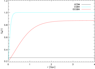
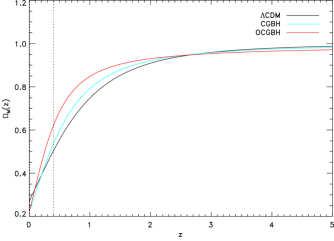
Figure 1: Upper panel: Present time (t=t₀) matter density parameters in the standard ($\Lambda$CDM, black line) and the void (GBH) cosmological models (red and cyan lines). Lower panel: Redshift evolution of the dimensionless matter density parameters in the standard ($\Lambda$CDM) and the void (GBH) cosmological models. The dotted vertical lines delimit the lowest redshift interval considered in the computation of the LF, at which the faint-end slopes are fit.

With those definitions, the angular diameter distance $A(r,t)$ can be computed in parametric form as,

$$A(r,t)=\frac{\Omega_{\scriptscriptstyle M}(r)}{2[1-\Omega_{\scriptscriptstyle M}(r)]^{3/2}}[\cosh(\eta)-1]\,A_{\scriptscriptstyle 0}(r),$$ (17)

where $A_{\scriptscriptstyle 0}(r)$ is the angular diameter distance at $t=t_{\scriptscriptstyle 0}$, and the parameter $\eta$ advances the solution given $r$, $t$, $H_{\scriptscriptstyle 0}(r)$, and $\Omega_{\scriptscriptstyle M}(r)$ as follows,

$$\sinh(\eta)-\eta=2\,\frac{[1-\Omega_{\scriptscriptstyle M}(r)]^{3/2}}{\Omega_{\scriptscriptstyle M}(r)}\,H_{\scriptscriptstyle 0}(r)\,t.$$ (18)

Once the angular diameter distance $d_{\scriptscriptstyle A}(z)=A[r(z),t(z)]$, is computed, we can use the very general reciprocity theorem (Etherington 1933),

$$d_{\scriptscriptstyle L}=(1+z)^{2}d_{\scriptscriptstyle A}=(1+z)d_{\scriptscriptstyle G},$$ (19)

to compute the luminosity distance $d_{\scriptscriptstyle L}(z)$ in the void models considered here. In the equation above, $d_{\scriptscriptstyle G}$ is the galaxy area distance, which reduces to the comoving distance in FLRW models. We still need to obtain the $r(z)$ and $t(z)$ relations in this Cosmology. We start with the radial null-geodesic equation, which can be written by making $ds^{2}=d\Omega^{2}=0$, yielding,

$$\left.\frac{dt}{dr}\right|_{{\textstyle{\scriptscriptstyle V}}}=-\frac{A^{\prime}(r,t)}{\sqrt{1-k(r)}},$$ (20)

where the minus sign is set for incoming light. The corresponding standard model equation reads,

$$\left.\frac{dt}{dr}\right|_{\scriptscriptstyle\Lambda}=-\frac{a(t)}{\sqrt{1-\kappa r^{2}}},$$ (21)

In the LTB metric, the time coordinate-redshift relation can be obtained to first order in wavelength starting from the redshift definition, as in, (e.g. Enqvist & Mattsson 2007),

$$\left.\frac{dt}{dz}\right|_{{\textstyle{\scriptscriptstyle V}}}=-\frac{1}{1+z}\frac{A^{\prime}}{\dot{A}^{\prime}},$$ (22)

whereas the corresponding $\Lambda$CDM relation can be written as,

$$\left.\frac{dt}{dz}\right|_{\scriptscriptstyle\Lambda}=-\frac{1}{1+z}\frac{a}{\dot{a}}.$$ (23)

The last two equations allow us to write the radial coordinate $r$ in terms of the redshift $z$, by solving the following expression,

$$\left.\frac{dr}{dz}\right|_{{\textstyle{\scriptscriptstyle V}}}=\frac{1}{1+z}\frac{\sqrt{1-k(r)}}{\dot{A}^{\prime}},$$ (24)

where $k(r)$ can be written in terms of the formerly defined quantities as,

$$k(r)=-\Omega_{\scriptscriptstyle k}\,H_{\scriptscriptstyle 0}^{2}(r)\,r^{2}.$$ (25)

Similarly, we can write, again for comparison,

$$\left.\frac{dr}{dz}\right|_{\scriptscriptstyle\Lambda}=\frac{1}{1+z}\frac{\sqrt{1-\kappa r^{2}}}{\dot{a}}.$$ (26)

It is worth noting that the comoving distance $r$ is not, in general, equal to the galaxy area distance, $d_{\scriptscriptstyle G}$, related to the luminosity distance through the reciprocity theorem (19).

The usual comoving-to-luminosity distance relation, $d_{\scriptscriptstyle G}=(1+z)\,d_{\scriptscriptstyle A}=r$, is only valid in the FLRW metric, for which the following relations holds,

$$(1+z)_{\scriptscriptstyle\Lambda}=\frac{a_{\scriptscriptstyle 0}}{a(t)},$$ (27)

$$d_{\scriptscriptstyle A,\Lambda}=r\,a(t),$$ (28)

where $a(t)$ is the usual scale factor, and $a_{\scriptscriptstyle 0}$, its value at present time (t=0). The last equation is valid only if we set $a_{\scriptscriptstyle 0}=1$. As a consequence, an LTB model with its luminosity distance-redshift relation constrained to fit the Hubble diagram for SNe Ia could still yield comoving distances, and therefore volumes, significantly different then those obtained in the standard model.

The additional constraint imposed by the measurements of the characteristic angular size of the Baryonic Accoustic Oscillations (BAO), (e.g. Percival et al. 2010; Reid et al. 2012), appears to pin down the comoving distance quite effectively up to intermediate redshifts, and it turns out that the difference in such distances computed in the $\Lambda$CDM and the GBH models is never larger than 10% at $z=1$. However, $r$ computed in the CGBH model at $z=5$ is approximately 12% smaller, and $\approx$ 17% in the open CGBH one.

The non-linear nature of the equations relating distances to volumes and luminosities, in particular for high redshift sources, must also be considered. At redshift $z=0.4$, for example, the luminosity distances computed in the void models, CGBH and OCGBH respectively, are 4.90% and 0.92% shorter then the standard model ones, whereas the comoving distances in the void models are 4.88% and 0.96% shorter when compared to the standard model value. Such differences correspond to an extra dimming in luminosities equal to 10.04% in the CGBH model and 1.85% in the OCGBH one. The corresponding shrink in volumes are 15.35% and 2.84%, for the CGBH and OCGBH models.

Such non-linearities that can make small discrepancies in luminosity and comoving distances caused by the central underdensity in GBH models sum up to non-negligible differences in the shape of the LF, when compared to the standard model. This can be understood by looking at Figure 2, where the luminosity distance and the comoving distance are plotted against the redshift.

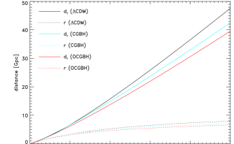
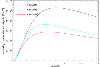
Figure 2: Upper panel: Luminosity (solid lines) and comoving distances (dotted lines) versus the redshift in the standard ($\Lambda$CDM) and the void (GBH) cosmological models. Up to redshift $z\approx 1$, both distances in the constrained, flat void model (CGBH) follow very closely their Standard Model counterparts, but even in the case of the best fit parameters in (Zumalacárregui et al. 2012) yield increasingly different distances with the redshift. Lower panel: Comoving volume elements in the standard ($\Lambda$CDM) and the void (GBH) cosmological models. The quantities in the void models adopted here, evolve with the redshift in a similar way as in the standard model, but at redshifts higher then approximately 0.6 their values are consistently lower then in the $\Lambda$CDM model.

For any given redshift $z^{\prime}$, consider the differences $\Delta d_{\scriptscriptstyle L}(z^{\prime})$ and $\Delta r(z^{\prime})$ between the distances computed in the standard model and those in the void models. Both differences depend on the redshift and do not, in general, cancel out or even yield a constant volume-to-luminosity ratio as a function of the redshift. As a result, the number of sources in each luminosity bin might change due to differences in the luminosities.

Additionally, the weight 1/V_max that each source add to the LF in that bin will not be the same, leading to a LF value in that luminosity bin in the void model that is different then the one in the standard model, even if the sources inside the bin are the same. Figure 2 shows the comoving volume element in the different cosmologies adopted here.

Such differences in the estimated value for the LF in each luminosity bin will not, in general, be the same. As a consequence, not only the normalization but also the shape of the LF might change from one cosmology to another.

4 Results

We compute the rest frame monochromatic and total IR luminosity LF for sources in the combined fields, blind selected in the 100 $\mu$m and 160 $\mu$m bands, using the non-parametric $1/V_{max}$ method, both in the Standard Model and the GBH void models. The LF values are listed in Tables 1-12, up to redshifts $z\approx 3$ for the monochromatic LFs and up to $z\approx 4$ for the total IR ones.

We use the same binning in luminosity and redshift as in (Gruppioni et al. 2013). The average values for the redshift intervals are 0.2, 0.6, 1.0, 1.5, 2.1, and 3.0, for the monochromatic LFs, and 0.2, 0.4, 0.5, 0.7, 0.9, 1.1, 1.5, 1.9, 2.2, 2.8 and 3.6 for the total IR ones. The effective wavelengths will be 60 and 90 $\mu$m in the rest-frame LF. Due to the lack of enough 1/V_max LF points to fit a Schechter function in the higher redshift bins, our analyses of the monochromatic luminosity functions is limited to intervals $\bar{z}\leq 3$. As a consistency check we compared our results for the standard model with Gruppioni et al.’s and the agreement is excellent.

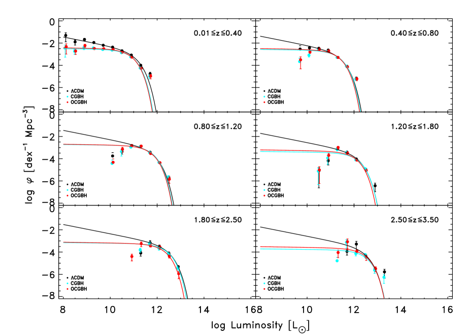
Figure 3: Luminosity functions derived in the standard ($\Lambda$CDM) (black dots) and the void (GBH) cosmological models (red and cyan dots). We show also the best-fit Schechter profiles to the rest-frame 100 $\mu$m 1/V_max corresponding to effective wavelengths of 60 $\mu$m.

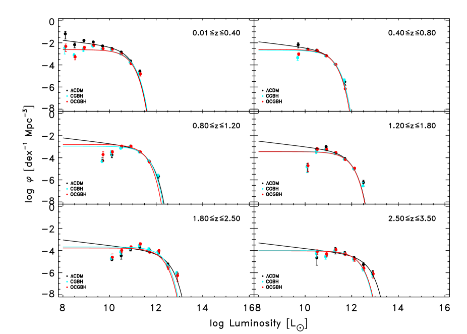
Figure 4: As Figure 3 for the rest-frame 160 $\mu$m 1/V_max luminosity functions. Here the effective wavelength is 90$\mu$m.

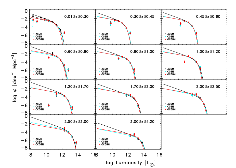
Figure 5: Schechter profile fits to the rest-frame total IR luminosity functions computed from the PACS 100 $\mu$m 1/V_max band, assuming the standard ($\Lambda$CDM) and the void (GBH) cosmological models.

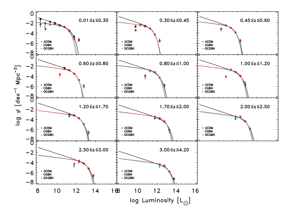
Figure 6: Schechter profile fits to the rest-frame total IR luminosity functions computed from the PACS 160 $\mu$m 1/V_max band, assuming the standard ($\Lambda$CDM) and the void (GBH) cosmological models.

The monochromatic and the total luminosity LFs are shown in Figures 3-6 for the three cosmologies considered in this paper. When comparing the values in each luminosity bin it is clear that in void cosmologies the density is lower at the lowest luminosities. While at redshift larger than 0.8 the incompleteness at low luminosities does not allow to draw any firm conclusion on this, in the two lowest redshift bins, the void models show LF values up to an order of magnitude lower than their $\Lambda$CDM counterpart, at L$\leq$10¹⁰L_⊙.

The resulting differences in the LF computed in different models show up at the faint luminosity end of the luminosity functions. We use the Schechter’s analytical profile (Schechter 1976),

$$\varphi(L)=\frac{\phi^{\scriptscriptstyle*}}{L^{\scriptscriptstyle*}}\,\left(\frac{L}{L^{\scriptscriptstyle*}}\right)^{\alpha}\,e^{-L/L^{\scriptscriptstyle*}}=\varphi^{\scriptscriptstyle*}\,\left(\frac{L}{L^{\scriptscriptstyle*}}\right)^{\alpha}\,e^{-L/L^{\scriptscriptstyle*}},$$ (29)

and fit it to the $1/V_{max}$ points over the ($\bar{z}$,$\bar{L}$) bins, where $\phi^{\scriptscriptstyle*}$ is the comoving number density normalisation, $L^{\scriptscriptstyle*}$ is the characteristic luminosity and $\alpha$ is the faint-end slope, using the IDL routine MPFITFUN (Markwardt 2009), based on the Levenberg-Marquardt algorithm (Moré 1978). For each best fit parameter, its formal 1-$\sigma$ uncertainty is obtained by taking the square root of its corresponding element in the diagonal of the 3x3 covariance matrix of the fitting procedure (see also Richter 1995).

Since we are primarily interested in checking possible changes in the LF caused by the underlying cosmologies, we chose to use the classical Schechter function, instead of the double exponential one (Saunders et al. 1990). The latter better fits the FIR LF bright-end, but the Schechter function have fewer free parameters, which allows it to fit higher redshift intervals, where the number of data points is small.

First we check for any variation of the $\alpha$ parameter with redshift, and find that it is consistent with no evolution. We test the incompleteness using the $V_{e}/V_{a}$ tests (Avni & Bahcall 1980). A given ($\bar{z}$,$\bar{L}$) bin is considered complete by this test if its $V_{e}/V_{a}$ value is 1/2. We find that the 1/V_max LF points do not suffer from significant incompleteness at $\bar{z}=0.2$ where the $V_{e}/V_{a}$ values in lowest luminosity bins of the monochromatic luminosity functions are 0.6 $\pm$ 0.1 and 0.5 $\pm$ 0.1 for the rest-frame 100 and 160 $\mu$m, respectively. Such values become 0.15 $\pm$ 0.09 and 0.22 $\pm$ 0.03 at $\bar{z}=1$, and 0.12 $\pm$ 0.05 and 0.11 $\pm$ 0.04 at $\bar{z}=3$.

This is because at higher redshifts the flux limit of the observations corresponds to increasingly different luminosity limits, depending on the SED of the sources, leading to an incompleteness in the lower luminosity bins that is dependent on the galaxy type (Ilbert et al. 2004). Because of this, in the fits presented in Tables 13-16, we chose to fix the $\alpha$ parameter to its value in the lower redshift interval.

5 Discussion

In Figures 3-6 we plot the $1/V_{\scriptscriptstyle max}$ LF estimations in the three different cosmologies, together with the best fit Schechter profiles for each of them. As can be seen on the four Figures, the faint end number densities in the void models are lower then the standard model ones.

If there was a direct correlation between the matter density parameter in the cosmology, and its estimated number density of sources selected in the FIR, then at the lowest redshift bin we should see higher number densities in the void models, since the $\Omega_{\scriptscriptstyle M}(z)$ in those models are bigger in that redshift range then the standard model value (more on that in Appendix A, Figure 1). The difference in the number densities at the lower redshift interval, for the different cosmologies, not only does not follow the same relation as the matter density parameters $\Omega_{\scriptscriptstyle M}(z)$, but also shows a dependence on the luminosity, being more pronounced at the fainter end in both the monocromatic and the total IR luminosity LFs. Such dependence produces significant differences in the faint-end slopes of the computed luminosity functions. That can only be attributed to the different geometrical parts of the cosmological models studied here, since the matter content, as discussed above, would only shift the normalization of the LF, independently of the luminosity of the sources.

In Table 17 we present the best fit values of $\alpha$ for each dataset / model combination. Simple error propagation allow us to write the uncertainty of the difference $\Delta\alpha$, between the faint-end slopes in the standard, $\alpha_{\scriptscriptstyle\Lambda}$, and the void, $\alpha_{\scriptscriptstyle V}$, models as,

$$\delta(\Delta\alpha)=\sqrt{(\delta\alpha_{\scriptscriptstyle\Lambda})^{2}\,+\,(\delta\alpha_{\scriptscriptstyle V})^{2}}.$$ (30)

The significance level of such difference can then be obtained by computing $\Delta\alpha/\delta(\Delta\alpha)$. For the monochromatic 100-$\mu$m luminosity functions, the difference between the $\alpha$ computed assuming the standard model and the ones computed in the GBH models studied here is 6.1-$\sigma$, as compared to its propagated uncertainty. For the monochromatic 160-$\mu$m luminosity functions, this value is 3.2-$\sigma$. For the total-IR 100-$\mu$ selected luminosity functions, these values are 2.9-$\sigma$ for the difference between $\Lambda$CDM and CGBH models, and 3.1-$\sigma$, for the $\Lambda$CDM-OCGBH difference. Finally, for the same differences in the total-IR 160-$\mu$m selected dataset, the significances are 3.1-$\sigma$, and 3.4-$\sigma$, respectively.

Could this difference be caused by a limitation of the $1/V_{\scriptscriptstyle max}$ method used here? As we show in the Appendix A, the matter density parameters in both $\Lambda$CDM and GBH models do not affect the performance of this LF estimator significantly: when the same input LF and matter density are assumed, the 1/V_max method obtains values within their error bars for all cosmological models considered. This indicates that this change in the slopes is caused by how the luminosities are computed from the redshifts in the different metrics.

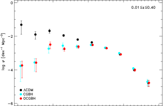
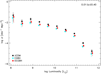
Figure 8: Upper panel: Effect of the luminosity distance - redshift relation on the shape of the LF. The black points were computed using the $1/V_{\scriptscriptstyle max}$ method, assuming both $d_{\scriptscriptstyle L}(z)$ and $r(z)$ relations stemming from the standard model, while the blue and red points kept the $r(z)$ relation for the $\Lambda$CDM model, changing only the $d_{\scriptscriptstyle L}(z)$ relation for that in the listed void model. The effect of the $d_{\scriptscriptstyle L}(z)$ relation on the shape of the LF is clear, especially at the lower luminosity bins. Lower panel: Effect of the comoving distance - redshift relation on the shape of the LF. The black points were computed using the $1/V_{\scriptscriptstyle max}$ method, assuming both $d_{\scriptscriptstyle L}(z)$ and $r(z)$ relations stemming from the standard model, while the blue and red points kept the $d_{\scriptscriptstyle L}(z)$ relation for the $\Lambda$CDM model, changing only the $r(z)$ relation for that in the listed void model. The effect of the $r(z)$ relation on the shape of the LF is found to be much less relevant then that of the $d_{\scriptscriptstyle L}(z)$ one.

To further check this assertion, we investigate the effects of both luminosity and comoving volume separately on the shape of the LF. Starting from the $1/V_{\scriptscriptstyle max}$ results for the LF in the interval 0 $<z<$ 0.4, assuming the standard cosmological model, we compute alternative LFs using the same methodology, but assuming either the luminosity distance of one of the void models and keeping the comoving distance of the standard model, or the luminosity distance of the standard model and the comoving distance of one of the void models. This allows us to assess how each distance definition affect the LF individually. The results are plotted in Figure 8, for the rest frame 100-$\mu m$ monochromatic luminosity dataset.

From those plots it is clear to see that the luminosity is the main cause of change in the shape of the LF. What remains to be investigated is whether the number density in a given luminosity bin is lower in the void models because of a re-arranging of the number counts in the luminosity bins, or because of a possible change in the maximum volume estimate of the sources in each bin. From this inspection, it turns out that the number counts in all three models are all within their Poisson errors, and therefore, the number densities in the void models are lower because the maximum volumes in them are larger.

Looking at equation (10), we identify two parameters that can introduce a dependency of the maximum volume of a source on its luminosity: the incompleteness corrections, $w_{\scriptscriptstyle k}(z)$, and the upper limit of the integral, $z_{\scriptscriptstyle max}$.

The incompleteness correction, $w_{\scriptscriptstyle k}(z)$, for each source, depends on the observed flux that source would have at that redshift, which is affected by the luminosity distance-redshift relation assumed.

More importantly though, at the higher luminosity bins, the $z_{\scriptscriptstyle max}$ of most of the sources there assumes the $z_{h}$ value for that redshift interval, which does not depend on the luminosity of the source. This renders the $V_{\scriptscriptstyle max}$ of the high luminosity sources approximately the same, apart from small changes caused by the incompleteness corrections $w_{\scriptscriptstyle k}$, as discussed above. At the lower luminosity bins, on the other hand, it happens more often that the $z_{\scriptscriptstyle max}$ of a source assumes its $\zeta$ value, which in this case depends on its luminosity, as it is clear from equation (8).

In order for that equation to hold, given that $f_{\scriptscriptstyle R}$ and $f_{\scriptscriptstyle R,lim}$ are fixed, the ratio between $d_{\scriptscriptstyle L}(z)/d_{\scriptscriptstyle L}(\zeta)$ must be the same for all cosmologies. Since the redshift $z$ of each source is also fixed, then it follows that the $\zeta$ value that makes the $d_{\scriptscriptstyle L}(z)/d_{\scriptscriptstyle L}(\zeta)$ ratio hold in the void models must be higher then in the standard model (see Figure 2). This, in turn, accounts for the larger maximum volumes, and lower number densities, at the low luminosity bins in the void models.

From the discussion above we conclude that a change in the luminosity distance - redshift relation changes the $z_{\scriptscriptstyle max}$ of the low luminosity sources, which in turn changes the maximum volumes, and finally, the fitted faint-end slope. However, from Figure 2, it is not obvious that such small differences in the $d_{\scriptscriptstyle L}(z)$ relation for the different cosmological models could cause such a significant change in the faint-end slopes, especially at low redshifts. It is useful to remind here that the LF is a non-linear combination of quantities that depend, from a geometrical point of view, on the luminosity distance (through the luminosities of the sources) and on the comoving distances (through their enclosing volumes). Even if the observational constraints on the luminosity-redshift relation, and the additional ones stemming from BAO results, yield both $d_{\scriptscriptstyle L}(z)$ and $r(z)$ quite robust under changes of the underlying cosmological models, such small differences in the distances could pile up non-linearly, and cause the observed discrepancies in the faint-end slope.

This appears to be the case here, at least in the low redshift interval where we can fit the faint-end slopes with confidence. Rather then following the trend of the matter density parameter, the number densities at those redshifts seem to be predominantly determined by their enclosing volumes (even if at low redshift the differences in the distance-redshift relations in the different cosmologies is quite small).

Looking at how the distances in Figure 2 have increasingly different values at higher redshifts, it would be interesting to check if the faint end slopes in the different cosmologies at some point start following that trend. Unfortunately, at higher redshifts the incompleteness caused by different luminosity limits for different populations does not allow us to draw any meaningful conclusion about the faint-end slope of the derived LFs. As it is, all that can be concluded is that the standard model LF would be over-estimating the local density of lower luminosity galaxies if the Universe’s expansion rate and history followed that of the LTB/GBH models.

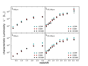
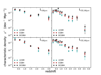
Figure 7: Upper panel: Redshift evolution of the characteristic luminosity $L^{\scriptscriptstyle\ast}$ on the four datasets of the present work. Lower panel: Redshift evolution of the characteristic luminosity $\phi^{\scriptscriptstyle\ast}$ on the same datasets.

We proceed to investigate the robustness with respect to the underlying cosmology of the redshift evolution of the other two Schechter parameters: the characteristic luminosity, $L^{\scriptscriptstyle\ast}$, and number density, $\phi^{\scriptscriptstyle\ast}$. Figure 7 present the redshift evolution of theses parameters, which we model by means of the simple relations:

$$L^{\scriptscriptstyle\ast}(z)\propto 10^{(1+z)A}$$ (31)

$$\phi^{\scriptscriptstyle\ast}(z)\propto 10^{(1+z)B}.$$ (32)

We use a least-squares technique to fit such evolution functions to their corresponding Schechter parameter results (Richter 1995). Table 18 lists the best fit values for the evolution parameters $A$ and $B$ in the different datasets / cosmologies.

The listed uncertainties for the evolution parameters are the formal 1-$\sigma$ values obtained from the square root of the corresponding diagonal element of the covariance matrix of the fit. We find no evidence for a significantly different evolution of either $L^{\scriptscriptstyle\ast}$ or $\phi^{\scriptscriptstyle\ast}$ in the void models considered. The monochromatic luminosities, specially the number density of sources in the rest-frame 160 $\mu$m, show some mild evidence of being affected by the geometrical effect discussed above, but the evolution parameters in the total IR are remarkably similar. We also note that assuming an open or flat CGBH model makes no significant difference to such parameters. It seems that those are more strongly affected by the intrinsic evolution of the sources, and the secular processes and merging history of galaxy formation, then the expansion rate of the Universe.

Physically speaking, in terms of tracing the redshift evolution of different galaxy populations using the FIR data in the present work, the marginally significant difference in the faint-end slopes, together with the evolution parameters for the characteristic number densities and luminosities, can be understood as follows: assertions about the number density of FIR low-luminosity galaxies, broadly related to populations that are poor in dust content, are still systematically affected by model-dependent corrections due to survey flux limits in the construction of the LF. That is, there might be less of those galaxies in the local Universe ($z\approx 0.3$), then what we expect based on the underlying standard model. On the other hand, evolution of the FIR high-luminosity end, broadly related to populations with high dust content, is well constrained by the flux limits of the PEP survey, where the underlying cosmological model is concerned.

6 Conclusions

In this work we have computed the far-IR luminosity functions for sources in the PEP survey, observed at the Herschel/PACS 100 and 160 $\mu$m bands. We computed both monochromatic and total IR luminosities assuming both the $\Lambda$CDM standard and GBH void cosmological models, with aims to assess how robust the luminosity functions are under a change of observationally constrained cosmologies.

We conclude that the current observational constraints imposed on any cosmological model by the combined set of SNe + CMB + BAO results are enough to yield robust estimates for the evolution of FIR characteristic luminosities $L^{\scriptscriptstyle\ast}$ and number densities, $\phi^{\scriptscriptstyle\ast}$.

We find, however, that estimations of the faint-end slope of the LF are still significantly dependent on the underlying cosmological model assumed, despite the before mentioned observational constraints. That is, if there is indeed an underdense region around the Galaxy, as predicted by the GBH models, causing the effective metric of the Universe at Gpc scale to be better fit by an LTB line element, then assuming the spatial homogeneous $\Lambda$CDM model in the computation of the LF would yield a over-estimated number density of faint galaxies, at least at lower redshifts (up to $z\approx 0.4$).

To answer the original question posed: the characteristic number density and the characteristic luminosity parameters of the FIR luminosity functions derived here are made robust by the present constraints on the cosmological model. The faint end slope, however, still show significant differences among the cosmologies studied here.

We show that those differences are caused mainly by slight discrepancies in the luminosity distance - redshift relation, still allowed by the observations. The 1/V_max methodology studied here is a necessary way to compute the LF using a flux limited survey like PEP. Such methodology, as we show, is not biased by the kind of under-dense regions proposed by the alternative cosmologies studied here. On the other hand, the necessary volume corrections intrinsic in the method are still dependent enough on the underlying assumptions about the geometry and expansion rate of the Universe at Gpc scale, to yield significant ($\approx$ 3-$\sigma$) discrepancies in their results. In other words, the “systematic” dispersion in the values of the low luminosity LF points, caused by the (arguably still) remaining degree of freedom in the choice of the underlying cosmological model, combined with the current flux limits, is still significantly larger then the statistic uncertainty assumed in the computation of the error bars of those points, causing the differences in the LF values to be larger then the combination of their computed uncertainties.

Surveys with lower flux limits would allow lower FIR-luminosity sources to be fully accounted for, reducing the marginally significant dependency of the FIR LF on the cosmological model still detected here.

Aknowledgements

AI is grateful to Takamitsu Miyagi and Karina Caputi, for the helpful tips on the building of luminosity functions, and Alan Heavens, for the insightful discussions on bayesian and Monte Carlo methods. Some Markov chain routines used at intermediate stages of this work were derived as a spin-off of a workshop at the Cape Town International Cosmology School, organized by the African Institute for Mathematical Sciences, between 15th and 28th of January, 2012. This work is jointly supported by Brazil’s CAPES and ESO studentships.

Table 1: Rest frame 100 $\mu$m 1/V_max Luminosity Function assuming the $\Lambda$CDM cosmological model. Units are dex^-1.Mpc^-3.

	Average redshift
Luminosity [L⊙]	0.2	0.6	1.0	1.5	2.1	3.0
5.0E+07	$(4.6\pm 3.3)\times 10^{-2}$
1.3E+08	$(4.9\pm 3.6)\times 10^{-2}$
3.2E+08	$(1.3\pm 0.6)\times 10^{-2}$
7.9E+08	$(2.1\pm 0.6)\times 10^{-2}$
2.0E+09	$(1.1\pm 0.2)\times 10^{-2}$
5.0E+09	$(6.4\pm 0.7)\times 10^{-3}$	$(2.9\pm 2.9)\times 10^{-3}$
1.3E+10	$(4.3\pm 0.4)\times 10^{-3}$	$(3.7\pm 1.5)\times 10^{-3}$	$(1.8\pm 1.8)\times 10^{-4}$
3.2E+10	$(2.01\pm 0.09)\times 10^{-3}$	$(3.4\pm 0.4)\times 10^{-3}$	$(4.4\pm 1.8)\times 10^{-4}$	$(7.9\pm 7.6)\times 10^{-6}$
7.9E+10	$(8.3\pm 0.5)\times 10^{-4}$	$(2.3\pm 0.2)\times 10^{-3}$	$(1.3\pm 0.2)\times 10^{-3}$	$(6.5\pm 3.8)\times 10^{-5}$
2.0E+11	$(1.0\pm 0.2)\times 10^{-4}$	$(5.2\pm 0.2)\times 10^{-4}$	$(1.3\pm 0.2)\times 10^{-3}$	$(8.0\pm 1.9)\times 10^{-4}$	$(8.1\pm 3.9)\times 10^{-5}$
5.0E+11	$(1.7\pm 0.7)\times 10^{-5}$	$(8.2\pm 0.7)\times 10^{-5}$	$(3.8\pm 0.4)\times 10^{-4}$	$(3.9\pm 0.6)\times 10^{-4}$	$(6.9\pm 3.8)\times 10^{-4}$	$(1.2\pm 0.6)\times 10^{-4}$
1.3E+12		$(6.8\pm 2.0)\times 10^{-6}$	$(4.4\pm 0.4)\times 10^{-5}$	$(9.3\pm 0.9)\times 10^{-5}$	$(3.1\pm 1.2)\times 10^{-4}$	$(5.2\pm 4.1)\times 10^{-4}$
3.2E+12			$(1.9\pm 0.8)\times 10^{-6}$	$(1.1\pm 0.2)\times 10^{-5}$	$(7.7\pm 2.6)\times 10^{-5}$	$(4.8\pm 1.5)\times 10^{-5}$
7.9E+12				$(3.7\pm 2.6)\times 10^{-7}$	$(4.8\pm 1.3)\times 10^{-6}$	$(3.3\pm 1.0)\times 10^{-6}$
2.0E+13						$(1.7\pm 1.2)\times 10^{-6}$

Table 2: Rest frame 100 $\mu$m 1/V_max Luminosity Function assuming the CGBH cosmological model. Units are dex^-1.Mpc^-3.

	Average redshift
Luminosity [L⊙]	0.2	0.6	1.0	1.5	2.1	3.0
5.0E+07	$(2.8\pm 1.6)\times 10^{-3}$
1.3E+08	$(3.6\pm 3.1)\times 10^{-3}$
3.2E+08	$(1.8\pm 0.8)\times 10^{-3}$
7.9E+08	$(3.8\pm 1.3)\times 10^{-3}$
2.0E+09	$(3.6\pm 0.9)\times 10^{-3}$
5.0E+09	$(2.7\pm 0.4)\times 10^{-3}$	$(2.2\pm 2.2)\times 10^{-4}$
1.3E+10	$(2.3\pm 0.2)\times 10^{-3}$	$(8.1\pm 2.5)\times 10^{-4}$	$(3.8\pm 3.8)\times 10^{-5}$
3.2E+10	$(1.4\pm 0.1)\times 10^{-3}$	$(2.6\pm 0.4)\times 10^{-3}$	$(4.3\pm 2.6)\times 10^{-4}$	$(7.6\pm 7.1)\times 10^{-6}$
7.9E+10	$(5.6\pm 0.4)\times 10^{-4}$	$(1.8\pm 0.2)\times 10^{-3}$	$(1.1\pm 0.2)\times 10^{-3}$	$(1.2\pm 0.8)\times 10^{-4}$
2.0E+11	$(5.7\pm 0.9)\times 10^{-5}$	$(5.1\pm 0.3)\times 10^{-4}$	$(1.1\pm 0.1)\times 10^{-3}$	$(7.2\pm 2.1)\times 10^{-4}$	$(1.5\pm 0.6)\times 10^{-4}$	$(1.6\pm 1.6)\times 10^{-5}$
5.0E+11	$(1.0\pm 0.4)\times 10^{-5}$	$(8.2\pm 0.7)\times 10^{-5}$	$(3.5\pm 0.4)\times 10^{-4}$	$(3.6\pm 0.5)\times 10^{-4}$	$(5.8\pm 2.1)\times 10^{-4}$	$(7.5\pm 5.3)\times 10^{-4}$
1.3E+12		$(5.9\pm 1.7)\times 10^{-6}$	$(4.7\pm 0.4)\times 10^{-5}$	$(7.8\pm 0.6)\times 10^{-5}$	$(2.2\pm 0.8)\times 10^{-4}$	$(7.2\pm 2.7)\times 10^{-5}$
3.2E+12			$(2.2\pm 0.9)\times 10^{-6}$	$(1.2\pm 0.2)\times 10^{-5}$	$(7.0\pm 2.1)\times 10^{-5}$	$(5.3\pm 2.2)\times 10^{-5}$
7.9E+12					$(3.8\pm 1.4)\times 10^{-6}$	$(2.4\pm 1.2)\times 10^{-6}$
2.0E+13						$(5.4\pm 3.9)\times 10^{-7}$

Table 3: Rest frame 100 $\mu$m 1/V_max Luminosity Function assuming the OCGBH cosmological model. Units are dex^-1.Mpc^-3.

	Average redshift
Luminosity [L⊙]	0.2	0.6	1.0	1.5	2.1	3.0
5.0E+07	$(2.2\pm 1.6)\times 10^{-3}$
1.3E+08	$(4.8\pm 3.8)\times 10^{-3}$
3.2E+08	$(1.9\pm 1.0)\times 10^{-3}$
7.9E+08	$(6.0\pm 1.8)\times 10^{-3}$
2.0E+09	$(3.2\pm 0.5)\times 10^{-3}$
5.0E+09	$(3.1\pm 0.4)\times 10^{-3}$	$(3.1\pm 2.6)\times 10^{-4}$
1.3E+10	$(2.7\pm 0.2)\times 10^{-3}$	$(1.6\pm 0.4)\times 10^{-3}$	$(4.7\pm 4.7)\times 10^{-5}$
3.2E+10	$(1.5\pm 0.2)\times 10^{-3}$	$(2.8\pm 0.4)\times 10^{-3}$	$(7.1\pm 3.4)\times 10^{-4}$	$(9.7\pm 9.1)\times 10^{-6}$
7.9E+10	$(5.4\pm 0.4)\times 10^{-4}$	$(2.0\pm 0.2)\times 10^{-3}$	$(1.5\pm 0.3)\times 10^{-3}$	$(2.0\pm 1.1)\times 10^{-4}$	$(4.0\pm 2.4)\times 10^{-5}$
2.0E+11	$(5.4\pm 0.9)\times 10^{-5}$	$(5.1\pm 0.3)\times 10^{-4}$	$(1.3\pm 0.2)\times 10^{-3}$	$(1.0\pm 0.3)\times 10^{-3}$	$(5.6\pm 2.5)\times 10^{-4}$	$(9.1\pm 6.0)\times 10^{-5}$
5.0E+11	$(1.1\pm 0.5)\times 10^{-5}$	$(7.2\pm 0.7)\times 10^{-5}$	$(2.9\pm 0.3)\times 10^{-4}$	$(3.3\pm 0.5)\times 10^{-4}$	$(3.7\pm 0.9)\times 10^{-4}$	$(8.5\pm 6.5)\times 10^{-4}$
1.3E+12		$(6.0\pm 1.9)\times 10^{-6}$	$(4.3\pm 0.5)\times 10^{-5}$	$(7.5\pm 0.6)\times 10^{-5}$	$(2.7\pm 0.9)\times 10^{-4}$	$(1.2\pm 0.4)\times 10^{-4}$
3.2E+12			$(1.4\pm 0.8)\times 10^{-6}$	$(8.8\pm 1.7)\times 10^{-6}$	$(4.2\pm 1.3)\times 10^{-5}$	$(3.3\pm 1.6)\times 10^{-5}$
7.9E+12					$(1.1\pm 0.7)\times 10^{-6}$	$(3.2\pm 1.5)\times 10^{-6}$
2.0E+13

Table 4: Rest frame 160 $\mu$m 1/V_max Luminosity Function assuming the $\Lambda$CDM cosmological model. Units are dex^-1.Mpc^-3.

	Average redshift
Luminosity [L⊙]	0.2	0.6	1.0	1.5	2.1	3.0
5.0E+07	$(4.9\pm 2.8)\times 10^{-2}$
1.3E+08	$(6.6\pm 4.3)\times 10^{-2}$
3.2E+08	$(6.7\pm 3.2)\times 10^{-3}$
7.9E+08	$(1.7\pm 0.5)\times 10^{-2}$
2.0E+09	$(1.2\pm 0.2)\times 10^{-2}$
5.0E+09	$(5.2\pm 0.6)\times 10^{-3}$	$(6.8\pm 3.3)\times 10^{-3}$	$(5.4\pm 5.4)\times 10^{-5}$
1.3E+10	$(3.0\pm 0.3)\times 10^{-3}$	$(2.7\pm 0.4)\times 10^{-3}$	$(1.8\pm 0.8)\times 10^{-4}$	$(1.8\pm 1.3)\times 10^{-5}$	$(1.5\pm 1.5)\times 10^{-5}$
3.2E+10	$(1.45\pm 0.07)\times 10^{-3}$	$(2.1\pm 0.2)\times 10^{-3}$	$(8.4\pm 1.5)\times 10^{-4}$	$(5.9\pm 2.3)\times 10^{-4}$	$(3.5\pm 1.8)\times 10^{-5}$	$(2.2\pm 1.8)\times 10^{-5}$
7.9E+10	$(2.3\pm 0.3)\times 10^{-4}$	$(7.0\pm 0.4)\times 10^{-4}$	$(1.1\pm 0.1)\times 10^{-3}$	$(9.6\pm 3.7)\times 10^{-4}$	$(1.2\pm 0.3)\times 10^{-4}$	$(3.5\pm 1.3)\times 10^{-5}$
2.0E+11	$(2.6\pm 0.9)\times 10^{-5}$	$(1.13\pm 0.08)\times 10^{-4}$	$(3.4\pm 0.4)\times 10^{-4}$	$(2.8\pm 0.4)\times 10^{-4}$	$(2.0\pm 0.5)\times 10^{-4}$	$(1.2\pm 0.7)\times 10^{-4}$
5.0E+11		$(3.0\pm 1.3)\times 10^{-6}$	$(5.0\pm 0.6)\times 10^{-5}$	$(8.6\pm 1.1)\times 10^{-5}$	$(1.2\pm 0.5)\times 10^{-4}$	$(6.1\pm 2.2)\times 10^{-5}$
1.3E+12			$(2.1\pm 0.9)\times 10^{-6}$	$(9.7\pm 1.6)\times 10^{-6}$	$(6.3\pm 1.9)\times 10^{-5}$	$(2.2\pm 0.6)\times 10^{-5}$
3.2E+12				$(5.8\pm 3.4)\times 10^{-7}$	$(6.0\pm 1.6)\times 10^{-6}$	$(5.5\pm 3.0)\times 10^{-6}$
7.9E+12					$(7.8\pm 3.5)\times 10^{-7}$	$(1.1\pm 0.5)\times 10^{-6}$
2.0E+13

Table 5: Rest frame 160 $\mu$m 1/V_max Luminosity Function assuming the CGBH cosmological model. Units are dex^-1.Mpc^-3.

	Average redshift
Luminosity [L⊙]	0.2	0.6	1.0	1.5	2.1	3.0
5.0E+07	$(2.3\pm 1.4)\times 10^{-3}$
1.3E+08	$(3.5\pm 2.6)\times 10^{-3}$
3.2E+08	$(7.8\pm 2.8)\times 10^{-4}$
7.9E+08	$(2.6\pm 1.0)\times 10^{-3}$
2.0E+09	$(5.3\pm 1.4)\times 10^{-3}$
5.0E+09	$(2.7\pm 0.4)\times 10^{-3}$	$(4.4\pm 1.8)\times 10^{-4}$	$(4.5\pm 4.5)\times 10^{-5}$
1.3E+10	$(2.4\pm 0.2)\times 10^{-3}$	$(2.3\pm 0.3)\times 10^{-3}$	$(2.9\pm 1.4)\times 10^{-4}$	$(1.5\pm 1.1)\times 10^{-5}$	$(2.0\pm 2.0)\times 10^{-5}$
3.2E+10	$(1.0\pm 0.1)\times 10^{-3}$	$(1.6\pm 0.2)\times 10^{-3}$	$(7.2\pm 1.2)\times 10^{-4}$	$(3.5\pm 1.2)\times 10^{-4}$	$(7.1\pm 2.9)\times 10^{-5}$	$(5.3\pm 2.8)\times 10^{-5}$
7.9E+10	$(1.8\pm 0.2)\times 10^{-4}$	$(6.5\pm 0.4)\times 10^{-4}$	$(1.1\pm 0.1)\times 10^{-3}$	$(5.7\pm 1.4)\times 10^{-4}$	$(1.5\pm 0.4)\times 10^{-4}$	$(2.8\pm 1.2)\times 10^{-5}$
2.0E+11	$(1.6\pm 0.5)\times 10^{-5}$	$(1.18\pm 0.08)\times 10^{-4}$	$(3.3\pm 0.4)\times 10^{-4}$	$(2.3\pm 0.3)\times 10^{-4}$	$(2.9\pm 0.7)\times 10^{-4}$	$(1.0\pm 0.4)\times 10^{-4}$
5.0E+11		$(4.1\pm 1.5)\times 10^{-6}$	$(5.1\pm 0.6)\times 10^{-5}$	$(7.2\pm 1.0)\times 10^{-5}$	$(1.2\pm 0.6)\times 10^{-4}$	$(5.6\pm 1.7)\times 10^{-5}$
1.3E+12			$(2.4\pm 1.0)\times 10^{-6}$	$(1.0\pm 0.2)\times 10^{-5}$	$(7.8\pm 2.6)\times 10^{-5}$	$(1.6\pm 0.5)\times 10^{-5}$
3.2E+12				$(2.9\pm 2.9)\times 10^{-7}$	$(4.3\pm 1.1)\times 10^{-6}$	$(2.2\pm 0.8)\times 10^{-6}$
7.9E+12					$(8.8\pm 4.4)\times 10^{-7}$	$(8.1\pm 4.1)\times 10^{-7}$
2.0E+13

Table 6: Rest frame 160 $\mu$m 1/V_max Luminosity Function assuming the OCGBH cosmological model. Units are dex^-1.Mpc^-3.

	Average redshift
Luminosity [L⊙]	0.2	0.6	1.0	1.5	2.1	3.0
5.0E+07	$(2.9\pm 1.8)\times 10^{-3}$
1.3E+08	$(4.7\pm 3.1)\times 10^{-3}$
3.2E+08	$(5.3\pm 2.4)\times 10^{-4}$
7.9E+08	$(3.7\pm 1.2)\times 10^{-3}$
2.0E+09	$(6.3\pm 1.6)\times 10^{-3}$
5.0E+09	$(3.0\pm 0.4)\times 10^{-3}$	$(9.7\pm 2.8)\times 10^{-4}$	$(2.0\pm 1.5)\times 10^{-4}$
1.3E+10	$(2.6\pm 0.2)\times 10^{-3}$	$(2.6\pm 0.4)\times 10^{-3}$	$(3.3\pm 1.2)\times 10^{-4}$	$(1.9\pm 1.4)\times 10^{-5}$	$(2.5\pm 2.5)\times 10^{-5}$
3.2E+10	$(1.08\pm 0.06)\times 10^{-3}$	$(2.0\pm 0.2)\times 10^{-3}$	$(1.1\pm 0.2)\times 10^{-3}$	$(6.2\pm 1.8)\times 10^{-4}$	$(1.0\pm 0.4)\times 10^{-4}$	$(8.2\pm 3.6)\times 10^{-5}$
7.9E+10	$(1.3\pm 0.2)\times 10^{-4}$	$(6.6\pm 0.4)\times 10^{-4}$	$(1.1\pm 0.1)\times 10^{-3}$	$(5.7\pm 1.5)\times 10^{-4}$	$(2.2\pm 0.5)\times 10^{-4}$	$(4.9\pm 2.2)\times 10^{-5}$
2.0E+11	$(1.5\pm 0.5)\times 10^{-5}$	$(1.07\pm 0.09)\times 10^{-4}$	$(3.4\pm 0.4)\times 10^{-4}$	$(3.0\pm 0.4)\times 10^{-4}$	$(4.1\pm 1.1)\times 10^{-4}$	$(1.2\pm 0.4)\times 10^{-4}$
5.0E+11		$(6.8\pm 6.8)\times 10^{-7}$	$(4.0\pm 0.5)\times 10^{-5}$	$(7.0\pm 0.7)\times 10^{-5}$	$(7.2\pm 1.3)\times 10^{-5}$	$(5.0\pm 1.5)\times 10^{-5}$
1.3E+12				$(1.1\pm 0.2)\times 10^{-5}$	$(9.5\pm 3.2)\times 10^{-5}$	$(1.7\pm 0.6)\times 10^{-5}$
3.2E+12					$(2.9\pm 1.0)\times 10^{-6}$	$(2.5\pm 0.9)\times 10^{-6}$
7.9E+12					$(5.5\pm 3.9)\times 10^{-7}$	$(7.8\pm 4.5)\times 10^{-7}$
2.0E+13

Table 7: Rest frame total IR 1/V_max Luminosity Function in the PACS 100 $\mu$m band, assuming the $\Lambda$CDM cosmological model. Units are dex^-1.Mpc^-3.

	Average redshift
Luminosity [L⊙]	0.2	0.4	0.5	0.7	0.9	1.1	1.5	1.9	2.2	2.8	3.6
1.8E+08	$(3.7\pm 2.8)\times 10^{-2}$
5.6E+08	$(1.3\pm 0.5)\times 10^{-2}$
1.8E+09	$(1.9\pm 0.5)\times 10^{-2}$
5.6E+09	$(9.3\pm 1.3)\times 10^{-3}$	$(1.0\pm 0.8)\times 10^{-3}$
1.8E+10	$(3.7\pm 0.3)\times 10^{-3}$	$(4.7\pm 1.1)\times 10^{-3}$	$(5.8\pm 3.4)\times 10^{-4}$				$(1.0\pm 1.0)\times 10^{-6}$
5.6E+10	$(1.46\pm 0.09)\times 10^{-3}$	$(2.8\pm 0.2)\times 10^{-3}$	$(2.9\pm 0.5)\times 10^{-3}$	$(1.3\pm 0.9)\times 10^{-2}$	$(5.6\pm 2.2)\times 10^{-4}$
1.8E+11	$(2.8\pm 0.4)\times 10^{-4}$	$(6.6\pm 0.4)\times 10^{-4}$	$(1.2\pm 0.1)\times 10^{-3}$	$(2.1\pm 0.2)\times 10^{-3}$	$(1.3\pm 0.2)\times 10^{-3}$	$(1.9\pm 0.5)\times 10^{-3}$	$(2.2\pm 1.2)\times 10^{-4}$
5.6E+11	$(2.0\pm 1.0)\times 10^{-5}$	$(4.6\pm 1.1)\times 10^{-5}$	$(1.2\pm 0.1)\times 10^{-4}$	$(2.7\pm 0.2)\times 10^{-4}$	$(5.3\pm 0.5)\times 10^{-4}$	$(6.6\pm 1.1)\times 10^{-4}$	$(6.7\pm 1.0)\times 10^{-4}$	$(2.2\pm 0.9)\times 10^{-4}$	$(2.3\pm 0.9)\times 10^{-4}$
1.8E+12	$(4.9\pm 4.9)\times 10^{-6}$	$(2.4\pm 2.4)\times 10^{-6}$	$(2.9\pm 2.1)\times 10^{-6}$	$(1.7\pm 0.4)\times 10^{-5}$	$(5.0\pm 0.5)\times 10^{-5}$	$(8.9\pm 0.7)\times 10^{-5}$	$(1.8\pm 0.2)\times 10^{-4}$	$(2.1\pm 0.5)\times 10^{-4}$	$(3.9\pm 1.2)\times 10^{-4}$	$(4.6\pm 3.3)\times 10^{-4}$
5.6E+12				$(1.5\pm 1.1)\times 10^{-6}$	$(1.7\pm 1.0)\times 10^{-6}$	$(6.1\pm 1.7)\times 10^{-6}$	$(1.2\pm 0.1)\times 10^{-5}$	$(3.9\pm 0.8)\times 10^{-5}$	$(6.8\pm 1.4)\times 10^{-5}$	$(9.8\pm 2.7)\times 10^{-5}$	$(2.8\pm 1.4)\times 10^{-5}$
1.8E+13							$(3.0\pm 2.1)\times 10^{-7}$	$(9.5\pm 4.7)\times 10^{-7}$	$(1.7\pm 0.5)\times 10^{-6}$	$(6.6\pm 1.6)\times 10^{-6}$	$(1.9\pm 0.7)\times 10^{-6}$

Table 8: Rest frame total IR 1/V_max Luminosity Function in the PACS 160 $\mu$m band, assuming the $\Lambda$CDM cosmological model. Units are dex^-1.Mpc^-3.

	Average redshift
Luminosity [L⊙]	0.2	0.4	0.5	0.7	0.9	1.1	1.5	1.9	2.2	2.8	3.6
1.8E+08	$(4.9\pm 3.5)\times 10^{-2}$
5.6E+08	$(7.7\pm 4.1)\times 10^{-3}$
1.8E+09	$(1.6\pm 0.4)\times 10^{-2}$
5.6E+09	$(9.0\pm 1.3)\times 10^{-3}$	$(1.8\pm 1.8)\times 10^{-3}$
1.8E+10	$(3.6\pm 0.3)\times 10^{-3}$	$(4.0\pm 1.0)\times 10^{-3}$	$(5.8\pm 2.7)\times 10^{-4}$
5.6E+10	$(1.51\pm 0.09)\times 10^{-3}$	$(2.5\pm 0.3)\times 10^{-3}$	$(2.8\pm 0.4)\times 10^{-3}$	$(4.2\pm 1.3)\times 10^{-3}$	$(1.1\pm 0.8)\times 10^{-4}$
1.8E+11	$(3.1\pm 0.4)\times 10^{-4}$	$(7.3\pm 0.5)\times 10^{-4}$	$(1.0\pm 0.1)\times 10^{-3}$	$(1.5\pm 0.2)\times 10^{-3}$	$(9.0\pm 1.5)\times 10^{-4}$	$(1.4\pm 0.3)\times 10^{-3}$	$(8.5\pm 3.4)\times 10^{-4}$
5.6E+11	$(2.1\pm 1.0)\times 10^{-5}$	$(4.9\pm 1.1)\times 10^{-5}$	$(1.3\pm 0.1)\times 10^{-4}$	$(2.9\pm 0.2)\times 10^{-4}$	$(6.1\pm 0.6)\times 10^{-4}$	$(7.4\pm 1.0)\times 10^{-4}$	$(5.2\pm 0.7)\times 10^{-4}$	$(1.6\pm 0.5)\times 10^{-4}$	$(1.6\pm 0.7)\times 10^{-4}$
1.8E+12	$(5.4\pm 5.4)\times 10^{-6}$	$(2.5\pm 2.5)\times 10^{-6}$	$(3.0\pm 2.1)\times 10^{-6}$	$(1.7\pm 0.4)\times 10^{-5}$	$(5.7\pm 0.6)\times 10^{-5}$	$(9.6\pm 0.7)\times 10^{-5}$	$(1.7\pm 0.2)\times 10^{-4}$	$(1.3\pm 0.3)\times 10^{-4}$	$(2.9\pm 0.5)\times 10^{-4}$	$(1.4\pm 0.6)\times 10^{-4}$	$(2.5\pm 1.6)\times 10^{-5}$
5.6E+12				$(1.5\pm 1.1)\times 10^{-6}$	$(1.7\pm 1.0)\times 10^{-6}$	$(6.3\pm 1.7)\times 10^{-6}$	$(1.4\pm 0.2)\times 10^{-5}$	$(3.6\pm 0.3)\times 10^{-5}$	$(4.4\pm 0.6)\times 10^{-5}$	$(7.7\pm 1.8)\times 10^{-5}$	$(2.5\pm 0.8)\times 10^{-5}$
1.8E+13							$(3.2\pm 2.3)\times 10^{-7}$	$(9.6\pm 4.8)\times 10^{-7}$	$(1.6\pm 0.5)\times 10^{-6}$	$(7.1\pm 1.1)\times 10^{-6}$	$(1.6\pm 0.5)\times 10^{-6}$

Table 9: Rest frame total IR 1/V_max Luminosity Function in the PACS 100 $\mu$m band, assuming the CGBH cosmological model. Units are dex^-1.Mpc^-3.

	Average redshift
Luminosity [L⊙]	0.2	0.4	0.5	0.7	0.9	1.1	1.5	1.9	2.2	2.8	3.6
1.8E+08	$(3.3\pm 3.1)\times 10^{-3}$
5.6E+08	$(2.0\pm 0.9)\times 10^{-3}$
1.8E+09	$(5.6\pm 1.4)\times 10^{-3}$
5.6E+09	$(3.9\pm 0.5)\times 10^{-3}$	$(6.0\pm 4.4)\times 10^{-4}$
1.8E+10	$(2.3\pm 0.2)\times 10^{-3}$	$(2.6\pm 0.6)\times 10^{-3}$	$(1.8\pm 1.8)\times 10^{-4}$				$(5.7\pm 5.7)\times 10^{-7}$
5.6E+10	$(1.1\pm 0.1)\times 10^{-3}$	$(2.2\pm 0.2)\times 10^{-3}$	$(2.4\pm 0.4)\times 10^{-3}$	$(4.2\pm 1.7)\times 10^{-3}$	$(5.3\pm 2.4)\times 10^{-4}$
1.8E+11	$(2.2\pm 0.3)\times 10^{-4}$	$(7.1\pm 0.4)\times 10^{-4}$	$(1.07\pm 0.09)\times 10^{-3}$	$(1.9\pm 0.2)\times 10^{-3}$	$(1.2\pm 0.2)\times 10^{-3}$	$(1.8\pm 0.5)\times 10^{-3}$	$(3.2\pm 1.7)\times 10^{-4}$
5.6E+11	$(1.2\pm 0.5)\times 10^{-5}$	$(4.8\pm 1.0)\times 10^{-5}$	$(1.5\pm 0.1)\times 10^{-4}$	$(3.0\pm 0.2)\times 10^{-4}$	$(5.7\pm 0.6)\times 10^{-4}$	$(6.8\pm 1.2)\times 10^{-4}$	$(6.1\pm 0.9)\times 10^{-4}$	$(2.9\pm 1.2)\times 10^{-4}$	$(2.2\pm 0.9)\times 10^{-4}$
1.8E+12	$(2.9\pm 2.9)\times 10^{-6}$	$(5.1\pm 3.6)\times 10^{-6}$	$(4.1\pm 2.3)\times 10^{-6}$	$(1.7\pm 0.4)\times 10^{-5}$	$(5.7\pm 0.6)\times 10^{-5}$	$(1.02\pm 0.09)\times 10^{-4}$	$(1.4\pm 0.1)\times 10^{-4}$	$(2.7\pm 0.8)\times 10^{-4}$	$(4.7\pm 1.2)\times 10^{-4}$	$(6.8\pm 4.2)\times 10^{-4}$	$(9.1\pm 9.1)\times 10^{-6}$
5.6E+12				$(1.6\pm 1.1)\times 10^{-6}$	$(1.8\pm 1.0)\times 10^{-6}$	$(7.3\pm 2.0)\times 10^{-6}$	$(1.2\pm 0.2)\times 10^{-5}$	$(4.4\pm 1.1)\times 10^{-5}$	$(5.4\pm 1.3)\times 10^{-5}$	$(8.7\pm 2.6)\times 10^{-5}$	$(3.0\pm 1.6)\times 10^{-5}$
1.8E+13							$(3.8\pm 2.7)\times 10^{-7}$	$(6.5\pm 4.6)\times 10^{-7}$	$(1.7\pm 0.6)\times 10^{-6}$	$(5.9\pm 1.6)\times 10^{-6}$	$(2.5\pm 0.9)\times 10^{-6}$

Table 10: Rest frame total IR 1/V_max Luminosity Function in the PACS 160 $\mu$m band, assuming the CGBH cosmological model. Units are dex^-1.Mpc^-3.

	Average redshift
Luminosity [L⊙]	0.2	0.4	0.5	0.7	0.9	1.1	1.5	1.9	2.2	2.8	3.6
1.8E+08	$(3.3\pm 2.8)\times 10^{-3}$
5.6E+08	$(1.7\pm 0.8)\times 10^{-3}$
1.8E+09	$(3.8\pm 1.2)\times 10^{-3}$
5.6E+09	$(5.0\pm 1.1)\times 10^{-3}$	$(2.9\pm 2.9)\times 10^{-4}$
1.8E+10	$(2.3\pm 0.2)\times 10^{-3}$	$(3.1\pm 0.8)\times 10^{-3}$	$(4.7\pm 2.4)\times 10^{-4}$
5.6E+10	$(1.3\pm 0.1)\times 10^{-3}$	$(1.7\pm 0.2)\times 10^{-3}$	$(2.5\pm 0.4)\times 10^{-3}$	$(2.3\pm 0.4)\times 10^{-3}$	$(8.9\pm 6.4)\times 10^{-5}$
1.8E+11	$(2.4\pm 0.3)\times 10^{-4}$	$(8.0\pm 0.5)\times 10^{-4}$	$(9.8\pm 1.2)\times 10^{-4}$	$(1.3\pm 0.2)\times 10^{-3}$	$(9.4\pm 1.9)\times 10^{-4}$	$(1.3\pm 0.2)\times 10^{-3}$	$(3.6\pm 1.3)\times 10^{-4}$
5.6E+11	$(1.2\pm 0.5)\times 10^{-5}$	$(5.1\pm 1.1)\times 10^{-5}$	$(1.5\pm 0.2)\times 10^{-4}$	$(3.3\pm 0.2)\times 10^{-4}$	$(5.9\pm 0.6)\times 10^{-4}$	$(7.6\pm 1.1)\times 10^{-4}$	$(5.3\pm 0.7)\times 10^{-4}$	$(2.4\pm 0.7)\times 10^{-4}$	$(2.1\pm 0.7)\times 10^{-4}$	$(1.9\pm 1.9)\times 10^{-5}$
1.8E+12	$(2.9\pm 2.9)\times 10^{-6}$	$(5.8\pm 4.1)\times 10^{-6}$	$(4.2\pm 2.4)\times 10^{-6}$	$(1.8\pm 0.4)\times 10^{-5}$	$(6.5\pm 0.7)\times 10^{-5}$	$(1.12\pm 0.09)\times 10^{-4}$	$(1.4\pm 0.1)\times 10^{-4}$	$(1.5\pm 0.4)\times 10^{-4}$	$(3.3\pm 0.6)\times 10^{-4}$	$(1.8\pm 0.5)\times 10^{-4}$	$(2.7\pm 1.4)\times 10^{-5}$
5.6E+12				$(1.7\pm 1.2)\times 10^{-6}$	$(1.9\pm 1.1)\times 10^{-6}$	$(7.4\pm 2.1)\times 10^{-6}$	$(1.4\pm 0.2)\times 10^{-5}$	$(4.4\pm 0.4)\times 10^{-5}$	$(4.1\pm 0.4)\times 10^{-5}$	$(7.7\pm 1.8)\times 10^{-5}$	$(2.9\pm 1.0)\times 10^{-5}$
1.8E+13							$(4.0\pm 2.8)\times 10^{-7}$	$(6.7\pm 4.7)\times 10^{-7}$	$(1.7\pm 0.6)\times 10^{-6}$	$(6.4\pm 1.3)\times 10^{-6}$	$(1.5\pm 0.4)\times 10^{-6}$

Table 11: Rest frame total IR 1/V_max Luminosity Function in the PACS 100 $\mu$m band, assuming the OCGBH cosmological model. Units are dex^-1.Mpc^-3.

	Average redshift
Luminosity [L⊙]	0.2	0.4	0.5	0.7	0.9	1.1	1.5	1.9	2.2	2.8	3.6
1.8E+08	$(4.7\pm 3.9)\times 10^{-3}$
5.6E+08	$(2.3\pm 1.1)\times 10^{-3}$
1.8E+09	$(6.7\pm 1.7)\times 10^{-3}$
5.6E+09	$(4.4\pm 0.6)\times 10^{-3}$	$(7.1\pm 5.3)\times 10^{-4}$
1.8E+10	$(2.6\pm 0.2)\times 10^{-3}$	$(3.5\pm 0.8)\times 10^{-3}$	$(7.4\pm 3.9)\times 10^{-4}$	$(9.2\pm 9.2)\times 10^{-4}$			$(7.3\pm 7.3)\times 10^{-7}$
5.6E+10	$(1.2\pm 0.2)\times 10^{-3}$	$(2.3\pm 0.2)\times 10^{-3}$	$(2.6\pm 0.4)\times 10^{-3}$	$(4.6\pm 1.9)\times 10^{-3}$	$(7.3\pm 3.1)\times 10^{-4}$	$(9.1\pm 9.1)\times 10^{-5}$
1.8E+11	$(1.9\pm 0.3)\times 10^{-4}$	$(7.0\pm 0.5)\times 10^{-4}$	$(1.2\pm 0.1)\times 10^{-3}$	$(2.2\pm 0.2)\times 10^{-3}$	$(1.5\pm 0.2)\times 10^{-3}$	$(2.4\pm 0.6)\times 10^{-3}$	$(4.9\pm 2.3)\times 10^{-4}$
5.6E+11	$(8.7\pm 4.4)\times 10^{-6}$	$(4.7\pm 1.1)\times 10^{-5}$	$(1.3\pm 0.2)\times 10^{-4}$	$(2.9\pm 0.2)\times 10^{-4}$	$(6.0\pm 0.6)\times 10^{-4}$	$(6.5\pm 1.1)\times 10^{-4}$	$(7.2\pm 1.0)\times 10^{-4}$	$(4.1\pm 1.5)\times 10^{-4}$	$(4.4\pm 1.6)\times 10^{-4}$
1.8E+12	$(3.4\pm 3.4)\times 10^{-6}$	$(3.0\pm 3.0)\times 10^{-6}$	$(3.3\pm 2.3)\times 10^{-6}$	$(1.7\pm 0.4)\times 10^{-5}$	$(4.7\pm 0.6)\times 10^{-5}$	$(1.03\pm 0.10)\times 10^{-4}$	$(1.5\pm 0.1)\times 10^{-4}$	$(3.1\pm 1.0)\times 10^{-4}$	$(4.5\pm 1.0)\times 10^{-4}$	$(8.8\pm 5.2)\times 10^{-4}$	$(1.9\pm 1.4)\times 10^{-5}$
5.6E+12				$(9.4\pm 9.4)\times 10^{-7}$	$(1.5\pm 1.1)\times 10^{-6}$	$(2.1\pm 1.2)\times 10^{-6}$	$(9.3\pm 1.6)\times 10^{-6}$	$(4.4\pm 1.4)\times 10^{-5}$	$(4.5\pm 1.0)\times 10^{-5}$	$(6.6\pm 2.1)\times 10^{-5}$	$(2.7\pm 1.7)\times 10^{-5}$
1.8E+13							$(2.3\pm 2.3)\times 10^{-7}$	$(8.1\pm 5.7)\times 10^{-7}$	$(1.5\pm 0.6)\times 10^{-6}$	$(5.1\pm 1.7)\times 10^{-6}$	$(2.9\pm 1.1)\times 10^{-6}$

Table 12: Rest frame total IR 1/V_max Luminosity Function in the PACS 160 $\mu$m band, assuming the OCGBH cosmological model. Units are dex^-1.Mpc^-3.

	Average redshift
Luminosity [L⊙]	0.2	0.4	0.5	0.7	0.9	1.1	1.5	1.9	2.2	2.8	3.6
1.8E+08	$(5.1\pm 3.6)\times 10^{-3}$
5.6E+08	$(6.2\pm 3.0)\times 10^{-4}$
1.8E+09	$(4.9\pm 1.4)\times 10^{-3}$
5.6E+09	$(5.8\pm 1.3)\times 10^{-3}$	$(3.4\pm 3.4)\times 10^{-4}$
1.8E+10	$(2.8\pm 0.3)\times 10^{-3}$	$(3.9\pm 1.0)\times 10^{-3}$	$(6.7\pm 3.1)\times 10^{-4}$	$(2.1\pm 1.5)\times 10^{-4}$
5.6E+10	$(1.3\pm 0.2)\times 10^{-3}$	$(1.9\pm 0.2)\times 10^{-3}$	$(3.1\pm 0.5)\times 10^{-3}$	$(2.9\pm 0.5)\times 10^{-3}$	$(1.1\pm 0.8)\times 10^{-4}$	$(7.6\pm 7.6)\times 10^{-5}$
1.8E+11	$(2.1\pm 0.3)\times 10^{-4}$	$(7.8\pm 0.5)\times 10^{-4}$	$(1.0\pm 0.1)\times 10^{-3}$	$(1.4\pm 0.2)\times 10^{-3}$	$(1.3\pm 0.2)\times 10^{-3}$	$(2.0\pm 0.3)\times 10^{-3}$	$(5.4\pm 1.8)\times 10^{-4}$
5.6E+11	$(9.1\pm 4.6)\times 10^{-6}$	$(5.1\pm 1.2)\times 10^{-5}$	$(1.3\pm 0.2)\times 10^{-4}$	$(3.1\pm 0.2)\times 10^{-4}$	$(6.3\pm 0.5)\times 10^{-4}$	$(6.4\pm 0.9)\times 10^{-4}$	$(6.3\pm 0.8)\times 10^{-4}$	$(3.4\pm 1.0)\times 10^{-4}$	$(3.5\pm 0.9)\times 10^{-4}$	$(4.8\pm 3.4)\times 10^{-5}$
1.8E+12	$(3.5\pm 3.5)\times 10^{-6}$	$(3.0\pm 3.0)\times 10^{-6}$	$(3.4\pm 2.4)\times 10^{-6}$	$(1.8\pm 0.4)\times 10^{-5}$	$(4.8\pm 0.6)\times 10^{-5}$	$(1.14\pm 0.10)\times 10^{-4}$	$(1.5\pm 0.1)\times 10^{-4}$	$(1.7\pm 0.3)\times 10^{-4}$	$(3.4\pm 0.6)\times 10^{-4}$	$(2.3\pm 0.6)\times 10^{-4}$	$(4.2\pm 1.8)\times 10^{-5}$
5.6E+12				$(1.0\pm 1.0)\times 10^{-6}$	$(1.7\pm 1.2)\times 10^{-6}$	$(2.2\pm 1.3)\times 10^{-6}$	$(1.0\pm 0.2)\times 10^{-5}$	$(3.8\pm 0.4)\times 10^{-5}$	$(4.1\pm 0.4)\times 10^{-5}$	$(6.1\pm 1.4)\times 10^{-5}$	$(2.4\pm 1.0)\times 10^{-5}$
1.8E+13							$(2.5\pm 2.5)\times 10^{-7}$	$(8.4\pm 5.9)\times 10^{-7}$	$(1.5\pm 0.6)\times 10^{-6}$	$(6.0\pm 1.3)\times 10^{-6}$	$(1.8\pm 0.5)\times 10^{-6}$

Table 13: Best fitting Schechter parameters for the rest frame 100 $\mu$m 1/V_max Luminosity functions.

	$\Lambda$CDM		CBGH		OCBGH
$\bar{z}$	$\varphi^{\scriptscriptstyle\ast}$	L∗	$\varphi^{\scriptscriptstyle\ast}$	L∗	$\varphi^{\scriptscriptstyle\ast}$	$L^{\scriptscriptstyle\ast}$
0.2	$(2.2\pm 0.2)\times 10^{-3}$	$(7.8\pm 0.7)\times 10^{10}$	$(2.7\pm 0.2)\times 10^{-3}$	$(5.2\pm 0.4)\times 10^{10}$	$(3.0\pm 0.3)\times 10^{-3}$	$(4.8\pm 0.4)\times 10^{10}$
0.6	$(1.8\pm 0.1)\times 10^{-3}$	$(1.81\pm 0.09)\times 10^{11}$	$(2.2\pm 0.1)\times 10^{-3}$	$(1.49\pm 0.06)\times 10^{11}$	$(2.5\pm 0.2)\times 10^{-3}$	$(1.36\pm 0.06)\times 10^{11}$
1.0	$(1.02\pm 0.09)\times 10^{-3}$	$(4.7\pm 0.2)\times 10^{11}$	$(1.5\pm 0.1)\times 10^{-3}$	$(3.7\pm 0.2)\times 10^{11}$	$(1.5\pm 0.1)\times 10^{-3}$	$(3.5\pm 0.2)\times 10^{11}$
1.5	$(4.1\pm 0.5)\times 10^{-4}$	$(9.9\pm 0.7)\times 10^{11}$	$(3.5\pm 0.4)\times 10^{-4}$	$(9.1\pm 0.8)\times 10^{11}$	$(4.6\pm 0.6)\times 10^{-4}$	$(7.4\pm 0.7)\times 10^{11}$
2.1	$(4.8\pm 1.4)\times 10^{-4}$	$(2.0\pm 0.2)\times 10^{12}$	$(5.6\pm 1.3)\times 10^{-4}$	$(1.6\pm 0.2)\times 10^{12}$	$(5.6\pm 1.2)\times 10^{-4}$	$(1.3\pm 0.1)\times 10^{12}$
3.0	$(2.8\pm 1.4)\times 10^{-4}$	$(2.0\pm 0.4)\times 10^{12}$	$(1.5\pm 0.5)\times 10^{-4}$	$(2.0\pm 0.3)\times 10^{12}$	$(2.2\pm 0.7)\times 10^{-4}$	$(1.9\pm 0.3)\times 10^{12}$

Table 14: Best fitting Schechter parameters for the rest frame 160 $\mu$m 1/V_max Luminosity functions.

	$\Lambda$CDM		CBGH		OCBGH
$\bar{z}$	$\varphi^{\scriptscriptstyle\ast}$	L∗	$\varphi^{\scriptscriptstyle\ast}$	L∗	$\varphi^{\scriptscriptstyle\ast}$	$L^{\scriptscriptstyle\ast}$
0.2	$(3.9\pm 0.4)\times 10^{-3}$	$(3.1\pm 0.3)\times 10^{10}$	$(2.4\pm 0.2)\times 10^{-3}$	$(3.3\pm 0.2)\times 10^{10}$	$(2.4\pm 0.2)\times 10^{-3}$	$(3.0\pm 0.1)\times 10^{10}$
0.6	$(2.3\pm 0.2)\times 10^{-3}$	$(7.2\pm 0.3)\times 10^{10}$	$(2.2\pm 0.2)\times 10^{-3}$	$(6.9\pm 0.3)\times 10^{10}$	$(2.5\pm 0.2)\times 10^{-3}$	$(6.2\pm 0.3)\times 10^{10}$
1.0	$(9.0\pm 0.8)\times 10^{-4}$	$(2.0\pm 0.1)\times 10^{11}$	$(1.12\pm 0.10)\times 10^{-3}$	$(1.65\pm 0.09)\times 10^{11}$	$(1.6\pm 0.1)\times 10^{-3}$	$(1.35\pm 0.06)\times 10^{11}$
1.5	$(3.9\pm 0.5)\times 10^{-4}$	$(3.7\pm 0.3)\times 10^{11}$	$(3.8\pm 0.4)\times 10^{-4}$	$(3.4\pm 0.2)\times 10^{11}$	$(3.5\pm 0.5)\times 10^{-4}$	$(3.4\pm 0.3)\times 10^{11}$
2.1	$(7.9\pm 1.5)\times 10^{-5}$	$(1.5\pm 0.2)\times 10^{12}$	$(2.1\pm 0.3)\times 10^{-4}$	$(8.3\pm 0.6)\times 10^{11}$	$(1.7\pm 0.3)\times 10^{-4}$	$(7.7\pm 0.8)\times 10^{11}$
3.0	$(3.8\pm 1.2)\times 10^{-5}$	$(2.1\pm 0.5)\times 10^{12}$	$(1.0\pm 0.2)\times 10^{-4}$	$(7.9\pm 1.1)\times 10^{11}$	$(9.3\pm 2.3)\times 10^{-5}$	$(8.4\pm 1.3)\times 10^{11}$

Table 15: Best fitting Schechter parameters for the rest frame total IR 1/V_max Luminosity functions in the PACS 100 $\mu$m band.

	$\Lambda$CDM		CBGH		OCBGH
$\bar{z}$	$\varphi^{\scriptscriptstyle\ast}$	L∗	$\varphi^{\scriptscriptstyle\ast}$	L∗	$\varphi^{\scriptscriptstyle\ast}$	$L^{\scriptscriptstyle\ast}$
0.2	$(9.9\pm 2.2)\times 10^{-4}$	$(1.6\pm 0.3)\times 10^{11}$	$(1.3\pm 0.2)\times 10^{-3}$	$(1.2\pm 0.2)\times 10^{11}$	$(1.9\pm 0.4)\times 10^{-3}$	$(8.7\pm 1.4)\times 10^{10}$
0.4	$(1.6\pm 0.2)\times 10^{-3}$	$(1.9\pm 0.2)\times 10^{11}$	$(2.0\pm 0.2)\times 10^{-3}$	$(1.7\pm 0.1)\times 10^{11}$	$(2.3\pm 0.2)\times 10^{-3}$	$(1.6\pm 0.1)\times 10^{11}$
0.5	$(1.4\pm 0.2)\times 10^{-3}$	$(2.9\pm 0.3)\times 10^{11}$	$(1.8\pm 0.2)\times 10^{-3}$	$(2.6\pm 0.2)\times 10^{11}$	$(2.3\pm 0.2)\times 10^{-3}$	$(2.2\pm 0.2)\times 10^{11}$
0.7	$(1.9\pm 0.3)\times 10^{-3}$	$(3.6\pm 0.4)\times 10^{11}$	$(1.5\pm 0.2)\times 10^{-3}$	$(4.0\pm 0.4)\times 10^{11}$	$(3.7\pm 0.5)\times 10^{-3}$	$(2.5\pm 0.2)\times 10^{11}$
0.9	$(6.4\pm 0.8)\times 10^{-4}$	$(8.7\pm 0.7)\times 10^{11}$	$(1.0\pm 0.1)\times 10^{-3}$	$(7.1\pm 0.5)\times 10^{11}$	$(1.5\pm 0.2)\times 10^{-3}$	$(5.7\pm 0.4)\times 10^{11}$
1.1	$(4.8\pm 1.0)\times 10^{-4}$	$(1.3\pm 0.2)\times 10^{12}$	$(9.7\pm 1.8)\times 10^{-4}$	$(9.1\pm 1.1)\times 10^{11}$	$(1.3\pm 0.2)\times 10^{-3}$	$(8.0\pm 0.8)\times 10^{11}$
1.5	$(3.9\pm 0.5)\times 10^{-4}$	$(2.0\pm 0.1)\times 10^{12}$	$(4.0\pm 0.5)\times 10^{-4}$	$(1.8\pm 0.1)\times 10^{12}$	$(5.9\pm 0.7)\times 10^{-4}$	$(1.5\pm 0.1)\times 10^{12}$
1.9	$(9.2\pm 2.1)\times 10^{-5}$	$(5.1\pm 0.7)\times 10^{12}$	$(2.4\pm 0.5)\times 10^{-4}$	$(3.5\pm 0.4)\times 10^{12}$	$(3.2\pm 0.8)\times 10^{-4}$	$(3.3\pm 0.5)\times 10^{12}$
2.2	$(8.4\pm 2.0)\times 10^{-5}$	$(5.9\pm 0.7)\times 10^{12}$	$(1.7\pm 0.4)\times 10^{-4}$	$(4.4\pm 0.5)\times 10^{12}$	$(3.1\pm 0.7)\times 10^{-4}$	$(3.5\pm 0.4)\times 10^{12}$
2.8	$(2.2\pm 0.8)\times 10^{-4}$	$(6.3\pm 1.1)\times 10^{12}$	$(2.8\pm 1.0)\times 10^{-4}$	$(5.2\pm 0.9)\times 10^{12}$	$(2.0\pm 0.8)\times 10^{-4}$	$(5.4\pm 1.1)\times 10^{12}$
3.6	$(3.8\pm 3.0)\times 10^{-6}$	$(2.4\pm 1.5)\times 10^{13}$	$(5.0\pm 5.9)\times 10^{-6}$	$(2.3\pm 2.6)\times 10^{13}$	$(1.4\pm 0.9)\times 10^{-5}$	$(1.2\pm 0.7)\times 10^{13}$

Table 16: Best fitting Schechter parameters for the rest frame total IR 1/V_max Luminosity functions in the PACS 160 $\mu$m band.

	$\Lambda$CDM		CBGH		OCBGH
$\bar{z}$	$\varphi^{\scriptscriptstyle\ast}$	L∗	$\varphi^{\scriptscriptstyle\ast}$	L∗	$\varphi^{\scriptscriptstyle\ast}$	$L^{\scriptscriptstyle\ast}$
0.2	$(1.1\pm 0.2)\times 10^{-3}$	$(1.6\pm 0.3)\times 10^{11}$	$(1.8\pm 0.3)\times 10^{-3}$	$(1.0\pm 0.2)\times 10^{11}$	$(2.5\pm 0.5)\times 10^{-3}$	$(7.9\pm 1.2)\times 10^{10}$
0.4	$(1.6\pm 0.2)\times 10^{-3}$	$(2.0\pm 0.2)\times 10^{11}$	$(2.0\pm 0.2)\times 10^{-3}$	$(1.8\pm 0.1)\times 10^{11}$	$(2.3\pm 0.2)\times 10^{-3}$	$(1.6\pm 0.1)\times 10^{11}$
0.5	$(1.3\pm 0.2)\times 10^{-3}$	$(2.9\pm 0.3)\times 10^{11}$	$(2.0\pm 0.2)\times 10^{-3}$	$(2.4\pm 0.2)\times 10^{11}$	$(2.6\pm 0.3)\times 10^{-3}$	$(2.1\pm 0.1)\times 10^{11}$
0.7	$(9.8\pm 1.2)\times 10^{-4}$	$(5.1\pm 0.5)\times 10^{11}$	$(1.3\pm 0.1)\times 10^{-3}$	$(4.4\pm 0.3)\times 10^{11}$	$(1.5\pm 0.2)\times 10^{-3}$	$(4.0\pm 0.4)\times 10^{11}$
0.9	$(5.1\pm 0.6)\times 10^{-4}$	$(1.01\pm 0.09)\times 10^{12}$	$(1.1\pm 0.1)\times 10^{-3}$	$(7.0\pm 0.5)\times 10^{11}$	$(1.7\pm 0.2)\times 10^{-3}$	$(5.5\pm 0.3)\times 10^{11}$
1.1	$(5.0\pm 0.8)\times 10^{-4}$	$(1.3\pm 0.1)\times 10^{12}$	$(1.1\pm 0.1)\times 10^{-3}$	$(8.6\pm 0.7)\times 10^{11}$	$(1.4\pm 0.2)\times 10^{-3}$	$(7.7\pm 0.6)\times 10^{11}$
1.5	$(3.2\pm 0.3)\times 10^{-4}$	$(2.2\pm 0.1)\times 10^{12}$	$(4.2\pm 0.4)\times 10^{-4}$	$(1.8\pm 0.1)\times 10^{12}$	$(5.6\pm 0.6)\times 10^{-4}$	$(1.5\pm 0.1)\times 10^{12}$
1.9	$(7.8\pm 1.1)\times 10^{-5}$	$(5.7\pm 0.6)\times 10^{12}$	$(2.2\pm 0.3)\times 10^{-4}$	$(3.6\pm 0.3)\times 10^{12}$	$(2.6\pm 0.4)\times 10^{-4}$	$(3.2\pm 0.4)\times 10^{12}$
2.2	$(9.6\pm 1.6)\times 10^{-5}$	$(5.6\pm 0.6)\times 10^{12}$	$(1.9\pm 0.3)\times 10^{-4}$	$(4.0\pm 0.4)\times 10^{12}$	$(3.1\pm 0.5)\times 10^{-4}$	$(3.1\pm 0.4)\times 10^{12}$
2.8	$(8.1\pm 2.4)\times 10^{-5}$	$(9.0\pm 1.5)\times 10^{12}$	$(1.9\pm 0.4)\times 10^{-4}$	$(5.8\pm 0.6)\times 10^{12}$	$(1.9\pm 0.4)\times 10^{-4}$	$(5.5\pm 0.6)\times 10^{12}$
3.6	$(1.4\pm 0.6)\times 10^{-5}$	$(1.0\pm 0.3)\times 10^{13}$	$(3.3\pm 1.2)\times 10^{-5}$	$(6.4\pm 1.2)\times 10^{12}$	$(4.9\pm 1.6)\times 10^{-5}$	$(5.8\pm 0.9)\times 10^{12}$

Table 17: Faint-end slopes values

dataset	$\Lambda$CDM	CGBH	OCGBH
$L_{\scriptscriptstyle 100\mu m}$	0.42 $\pm$ 0.04	0.03 $\pm$ 0.05	0.03 $\pm$ 0.05
$L_{\scriptscriptstyle 160\mu m}$	0.25 $\pm$ 0.06	0.00 $\pm$ 0.05	0.00 $\pm$ 0.05
$L_{\scriptscriptstyle IR,100\mu m}$	0.67 $\pm$ 0.06	0.38 $\pm$ 0.08	0.33 $\pm$ 0.09
$L_{\scriptscriptstyle IR,160\mu m}$	0.61 $\pm$ 0.07	0.26 $\pm$ 0.09	0.2 $\pm$ 0.1

Table 18: Comoving number density and characteristic luminosity evolution parameters.

dataset	model	$A$	$B$
	$\Lambda$CDM	$(5.2\pm 1.0)\times 10^{-1}$	$(-3.3\pm 0.6)\times 10^{-1}$
$L_{\scriptscriptstyle 100\mu m}$	CGBH	$(5.6\pm 1.0)\times 10^{-1}$	$(-4.5\pm 0.8)\times 10^{-1}$
	OCGBH	$(5.5\pm 0.9)\times 10^{-1}$	$(-4.2\pm 0.7)\times 10^{-1}$
	$\Lambda$CDM	$(6.8\pm 0.8)\times 10^{-1}$	$(-7.6\pm 0.6)\times 10^{-1}$
$L_{\scriptscriptstyle 160\mu m}$	CGBH	$(5.4\pm 0.9)\times 10^{-1}$	$(-5.8\pm 0.8)\times 10^{-1}$
	OCGBH	$(5.4\pm 0.9)\times 10^{-1}$	$(-5.8\pm 0.8)\times 10^{-1}$
	$\Lambda$CDM	$(6.4\pm 0.5)\times 10^{-1}$	$(-6.6\pm 1.0)\times 10^{-1}$
$L_{\scriptscriptstyle IR,100\mu m}$	CGBH	$(6.4\pm 0.4)\times 10^{-1}$	$(-6.3\pm 0.9)\times 10^{-1}$
	OCGBH	$(6.3\pm 0.5)\times 10^{-1}$	$(-6.1\pm 0.7)\times 10^{-1}$
	$\Lambda$CDM	$(5.8\pm 0.7)\times 10^{-1}$	$(-5.9\pm 0.5)\times 10^{-1}$
$L_{\scriptscriptstyle IR,160\mu m}$	CGBH	$(5.6\pm 0.7)\times 10^{-1}$	$(-5.1\pm 0.3)\times 10^{-1}$
	OCGBH	$(5.6\pm 0.7)\times 10^{-1}$	$(-5.1\pm 0.3)\times 10^{-1}$

Appendix A Mock Catalogues

In this appendix we test whether the 1/V_max LF estimator is reliable in studying Gpc scale voids like the ones proposed by the GBH models, embedded in an LTB dust model. We follow the general approach by (Takeuchi et al. 2000) who made use of mock catalogues that were built assuming a (non-central and small) void with a radius of 1.6 Mpc at a distance of 0.8 Mpc, and at a limiting redshift of $z=0.1$. Our mock catalogues are built using the matter density distributions in the GBH models, as shown in Figure 1. Also, the redshift range of our interest is 4 times larger, since we want to test the validity of the estimator in the interval $\Delta z=[0.01,0.4]$, where we fit the faint-end slope of the luminosity functions.

Mock catalogues are built reproducing the detection limits and SED distributions in the GOODS-S and COSMOS fields, in the PACS 100 and 160 $\mu$m filters, as listed in (Gruppioni et al. 2013). We chose those two fields for better representing the whole of the data used in this work: GOODS-S is the field with the lowest flux limits in the PEP survey, while COSMOS is the one with the widest effective area.

Naively one might decide to use matter density distributions in Figure 1 to randomly assign comoving distances to the sources in the mock catalogue. However, given the large redshift interval we aim to cover in our simulations, the redshift evolution of the density profiles must be fully considered.

For each of the present time, rest-frame (z=0) matter density profile, $\Omega_{\scriptscriptstyle M}(r)$, defined in a constant time coordinate hipersurface, and fit by both the standard model and the void models (see Figure 1), we compute the corresponding redshift evolution, $\Omega_{\scriptscriptstyle M}(z)$, defined in the past light-cone of the same cosmological model. In the FLRW spacetime, the dimensionless density parameters $\Omega_{\scriptscriptstyle M}$ and $\Omega_{\scriptscriptstyle M}(z)$ are related as follows:

$$\Omega_{\scriptscriptstyle M}(z)=\Omega_{\scriptscriptstyle M}\left[\frac{H_{\scriptscriptstyle 0}}{H(z)}\right]^{2}a(z)^{-3},$$ (33)

where $H(z)$ is the Hubble parameter at redshift $z$, carried over from the definition of the critical density $\rho_{\scriptscriptstyle c}=3H_{\scriptscriptstyle 0}^{2}/8\pi G$, and $a(z)$ the scale factor, both as functions of the redshift. Similarly, following the definition of $\Omega_{\scriptscriptstyle M}(r)$ used in GBH and (Zumalacárregui et al. 2012), one may write an analogue equation in the void-LTB models as,

$$\Omega_{\scriptscriptstyle M}(z)=\Omega_{\scriptscriptstyle M}[r(z)]\left\{\frac{H_{\scriptscriptstyle\perp 0}[r(z)]}{H_{\scriptscriptstyle\perp}[t(z),r(z)]}\right\}^{2}a_{\scriptscriptstyle\perp}[t(z),r(z)]^{-3},$$ (34)

where $H_{\scriptscriptstyle\perp}[t(z),r(z)]$ and $a_{\scriptscriptstyle\perp}[t(z),r(z)]$ are now the transverse Hubble parameter and scale factor, respectively. Figure 1 shows the redshift evolution of the density parameters in the three models considered in the present work. Note, however, that there’s an ambiguity in the definition of equation (34), due to the fact that the LTB geometry possesses radial expansion rate and scale factor that are in general different from their transverse counterparts. For the purpose of building mock catalogues that are consistent with the void-LTB parametrizations used in this work, we chose to use the transverse quantities, because those were the ones used in (Zumalacárregui et al. 2012), from where the best fit parameters used in this work were taken.

Next, we randomly assign: a. redshifts using a probability distribution based on one of those $\Omega_{\scriptscriptstyle M}(z)$ profiles; b. rest-frame luminosities, based on an input Schechter LF with parameters L^∗=10¹¹ L_☉, $\phi^{*}$=10^-3 dex^-1.Mpc^-3 and $\alpha$ = -1/2; and c. a representative empirical SED from the Poletta templates, drawn from the same distributions reported in (Gruppioni et al. 2013). In this way, we can test first the validity of the 1/V_max estimator itself for the purposes of the present work, and second, the possible effects of the different predicted density profiles on the values recovered of the LF.

Having assigned a redshift, a luminosity and a SED for each Monte Carlo (MC) realisation, we proceed to compute k-corrections and fluxes, using the luminosity distance-redshift relation consistent with the cosmology assumed for the redshift assignment. We include the source in the mock catalogue if its observed flux is larger than the detection limit of the field. We repeat such process until we have a catalogue with a number of selected MC realisations equal to the number of sources in the redshift interval $\Delta z=[0.01,0.4]$, for a given field.

We then compute the 1/V_max LF following the same methodology described in §2.3, using 100 mock catalogues built as above. To assess the goodness-of-fit of the 1/V_max LF versus the input Schechter profile, we compute the one-sided Kolmogorov-Smirnov (KS) statistic of the normalised residuals against a Gaussian with zero mean and unit variance. We plot the 1/V_max points computed using the mock catalogues against the input Schechter LF used in their build-up in Figures 9, 10, and 11 The KS statistic for each mock/input comparison is listed between parentheses, in the plots. The smaller this value, the closer the normalized residuals are to a gaussian with zero mean and unit variance.

We find that the matter density parameter profiles of interest don’t change significantly the LF results, as can be seen by comparing different panels in a same Figure. We note what appears to be a general bias towards under-estimating the characteristic luminosity $L^{\ast}$, in agreement with (Smith 2012) results.

Comparison between the $1/V_{\scriptscriptstyle max}$ LF results for the GOODS-S mocks built using either the present time density profiles (Figure 9) or the appropriate redshift evolution of those (Figure 10), shows that the method successfully takes into consideration the redshift distortion in the matter distribution, yielding points in both cases that recover the input LF profile qualitatively close in respect to each other, with respect to their KS statistics.

Comparison between the mocks for the GOODS-S (Figure 10) and COSMOS (Figure 11) fields built using the redshift evolution of the density parameter in the different cosmological models shows that the $1/V_{\scriptscriptstyle max}$ estimator fares slightly better in the deeper GOODS-S field, as compared to the wider COSMOS one.

Summing up, even if the method is not perfectly robust under a change in the cosmological model, the variations caused by a change in the underlying cosmology in the results obtained with the $1/V_{\scriptscriptstyle max}$ estimator are not enough to explain the significant differences in the shape of the LF at the considered redshift interval, $\Delta z=[0.01,0.4]$.

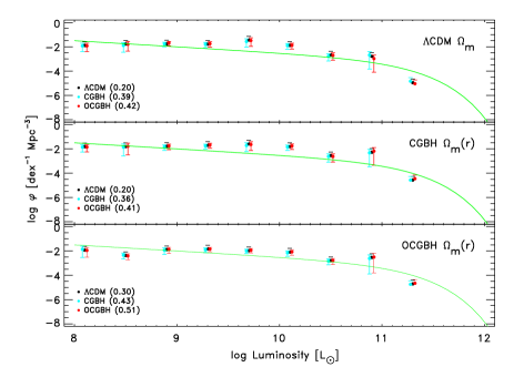
Figure 9: Results for the 1/V_max LF estimator, computed from mock catalogues assuming a constant density profile $\Omega_{\scriptscriptstyle M}=0.27$ ($\Lambda$CDM), and the underdense profiles of equation (15) for the GBH void models (Figure 1). Sources luminosities in the mock catalogue are drawn from the Schechter LF (here shown in green dashed line, with parameters L^∗=10¹¹ L_☉, $\varphi^{*}$=10^-3 dex^-1.Mpc^-3 and $\alpha$ = -1/2). Flux limits and SED are taken from the results of (Gruppioni et al. 2013) for the PEP survey dataset in the GOODS-S field.

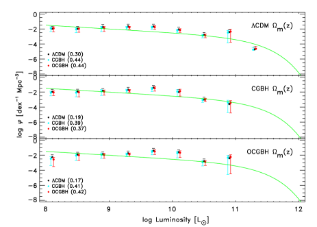
Figure 10: Same as Figure 9 but assuming the redshift evolution of the matter density profiles in both the standard ($\Lambda$CDM), and the void-LTB models as in Figure 1.

Figure 11: Same as Figure 10 but for the PEP survey dataset in the COSMOS field.

References

- Albani et al. (2007) Albani, V. V. L., Iribarrem, A. S., Ribeiro, M. B., & Stoeger, W. R. 2007, ApJ, 657, 760
- Alfedeel & Hellaby (2010) Alfedeel, A. H. A. & Hellaby, C. 2010, General Relativity and Gravitation, 42, 1935
- Arnouts et al. (1999) Arnouts, S., Cristiani, S., Moscardini, L., et al. 1999, MNRAS, 310, 540
- Avni & Bahcall (1980) Avni, Y. & Bahcall, J. N. 1980, ApJ, 235, 694
- Babbedge et al. (2006) Babbedge, T. S. R., Rowan-Robinson, M., Vaccari, M., et al. 2006, MNRAS, 370, 1159
- Benson et al. (2003) Benson, A. J., Bower, R. G., Frenk, C. S., et al. 2003, ApJ, 599, 38
- Berta et al. (2010) Berta, S., Magnelli, B., Lutz, D., et al. 2010, A&A, 518, L30
- Berta et al. (2011) Berta, S., Magnelli, B., Nordon, R., et al. 2011, A&A, 532, A49
- Blanton & Roweis (2007) Blanton, M. R. & Roweis, S. 2007, AJ, 133, 734
- Bolejko et al. (2011a) Bolejko, K., Célérier, M.-N., & Krasiński, A. 2011a, Classical and Quantum Gravity, 28, 164002
- Bolejko et al. (2011b) Bolejko, K., Hellaby, C., & Alfedeel, A. H. A. 2011b, J. Cosmology Astropart. Phys., 9, 11
- Boylan-Kolchin et al. (2009) Boylan-Kolchin, M., Springel, V., White, S. D. M., Jenkins, A., & Lemson, G. 2009, MNRAS, 398, 1150
- Bull & Clifton (2012) Bull, P. & Clifton, T. 2012, Phys. Rev. D, 85, 103512
- Bull et al. (2012) Bull, P., Clifton, T., & Ferreira, P. G. 2012, Phys. Rev. D, 85, 024002
- Busti & Lima (2012) Busti, V. C. & Lima, J. A. S. 2012, MNRAS, L504
- Caputi et al. (2007) Caputi, K. I., Lagache, G., Yan, L., et al. 2007, ApJ, 660, 97
- Célérier (2007) Célérier, M.-N. 2007, New Advances in Physics, 1, 29
- Clarkson et al. (2011) Clarkson, C., Ellis, G., Larena, J., & Umeh, O. 2011, Rept. Prog. Phys., 74, 112901
- Clarkson et al. (2012) Clarkson, C., Ellis, G. F. R., Faltenbacher, A., et al. 2012, MNRAS, 426, 1121
- Clarkson & Umeh (2011) Clarkson, C. & Umeh, O. 2011, Classical and Quantum Gravity, 28, 164010
- Clifton et al. (2012) Clifton, T., Rosquist, K., & Tavakol, R. 2012, Phys. Rev. D, 86, 043506
- Cool et al. (2012) Cool, R. J., Eisenstein, D. J., Kochanek, C. S., et al. 2012, ApJ, 748, 10
- Datta et al. (2012) Datta, K. K., Mellema, G., Mao, Y., et al. 2012, MNRAS, 3286
- de Putter et al. (2012) de Putter, R., Verde, L., & Jimenez, R. 2012, ArXiv e-prints, astro-ph.CO 1208.4534
- Ellis (2011) Ellis, G. F. R. 2011, Classical and Quantum Gravity, 28, 164001
- Enqvist & Mattsson (2007) Enqvist, K. & Mattsson, T. 2007, J. Cosmology Astropart. Phys., 2, 19
- Etherington (1933) Etherington, I. M. H. 1933, Philosophical Magazine, 15, 761, reprinted in Gen. Rel. Grav., 39, 1055, 2007
- February et al. (2010) February, S., Larena, J., Smith, M., & Clarkson, C. 2010, MNRAS, 405, 2231