Interplay of Superconductivity and Spin-Dependent Disorder

Abstract

The finite temperature phase diagram for the 2D attractive fermion Hubbard model with spin-dependent disorder is considered within Bogoliubov-de Gennes mean field theory. Three types of disorder are studied. In the first, only one species is coupled to a random site energy; in the second, the two species both move in random site energy landscapes which are of the same amplitude, but different realizations; and finally, in the third, the disorder is in the hopping rather than the site energy. For all three cases we find that, unlike the case of spin-symmetric randomness, where the energy gap and average order parameter do not vanish as the disorder strength increases, a critical disorder strength exists separating distinct phases. In fact, the energy gap and the average order parameter vanish at distinct transitions, $V_{c}^{\rm gap}$ and $V_{c}^{\rm op}$, allowing for a gapless superconducting (gSC) phase. The gSC phase becomes smaller with increasing temperature, until it vanishes at a temperature $T^{\ast}$.

I Introduction

The study of disordered electronic systems is of major interest in condensed matter physics lee85 ; belitz94 because randomness breaks translational invariance and leads to localized electron states. In noninteracting systems, typically all the states are localized in one and two dimensions, even by small amounts of disorder abrahams79 , while in three dimensions, states with large and small energies are localized, and a ‘mobility edge’ separates these from extended states near the center of the energy distribution. In real materials, disorder can arise from vacancies or impurity atoms, dislocations, and other forms of structural imperfections.

The effect of interparticle interactions on these localized and extended states has proven to be a very challenging problem. Experiments using silicon MOSFETS of very high purity now suggest kravchenko94 ; popovic97 ; abrahams00 that repulsive interactions might allow a metallic phase to exist in two dimensions. An equally interesting set of questions concerns the interplay of disorder and attractive interactions, and the occurrence of superconductor-insulator transitions. One well-studied issue is the existence of a universal conductivity in thin films arwhite86 ; orr86 ; fisher90 ; hebard94 .

Recently it has become possible to address the interplay of randomness and interactions within a new experimental context, namely that of ultracold fermionic and bosonic atomic gases confined to optical lattices jaksch98 ; bloch08 . Here the role of ‘spin’ is played by atoms in different hyperfine states. Disorder can be superimposed on the periodic optical lattices created by interfering counter-propagating lasers by means of the introduction of speckle fieldsaspect09 ; palencia10 . This randomness can now be made on the scale of the lattice constant. Interactions between the atoms can be tuned through a Feshbach resonancechin10 and can be either repulsive or attractive.

Optical lattice experiments do not just represent a new realization of model Hamiltonians of interacting and disordered materialswhite09 ; zhou10 ; they also allow the study of situations which would be more difficult to achieve in the solid state. One possibility is “spin”-dependent disorder in which atoms of different hyperfine structures do not see the same random potential, a natural follow-on to existing experiments where the optical lattice itself is spin-dependentdemarco11 ; demarco10 ; mandel03 ; feiguin09 ; liu04 .

In this paper we present a detailed theoretical study of such spin-dependent disorder. We consider the attractive fermion Hubbard model in two dimensions, which has a low temperature superconducting phase, and include three types of spin-dependent disorder: 1) random potential on the up-spin but zero potential on the down-spin; 2) random potential of the same strength but different realizations on each spin species; 3) random hopping energies of the same strength, but again with different realizations on each spin species.. We study these cases with finite-temperature Bogoliubov-de Gennes (BdG) mean-field theorydegennes66 . This BdG approach to the $-|U|$ Hubbard model allows us to examine the strong interaction and strong disorder regimes which are beyond the realm of validity of Anderson’s theoremanderson59 . The mean-field approximation of course ignores fluctuations. Some of the effects of extending beyond the mean-field are explored in Ref. ghosal98, ; ghosal01, .

Our key results are as follows: [1] Unlike the case of spin independent randomness, for which BdG theory produces no transition as the disorder strength is increased, we show here that spin dependence produces a vanishing of the superconducting order parameter $\Delta_{\rm op}$ and energy gap $E_{\rm gap}$; [2] The critical points can be different for $\Delta_{\rm op}$ and $E_{\rm gap}$, leading to a gapless superconducting phase; and [3] models with different types of spin-dependent disorder behave in a qualitatively similar manner. Results at zero temperature for this problem can also be found in Ref. jiang11, .

We begin with a description of the model and method in Section II, and present our most central results, the phase diagrams, in Section III. Several additional details of the properties of these models are summarized in Section IV. Section V contains some concluding remarks. The rest of this introduction will provide more details for the experimental prospects for realizing spin-dependent disordered optical lattices.

Spin-independent disorder in a 3D optical lattice has been studied in the context of the disordered Bose-Hubbard model in Refs. white09, ; pasienski10, . The phase diagram was determined through transport properties. Non-interacting fermions in a spin-independent disordered 3D lattice have also been realizedkondov11 and used to demonstrate Anderson localization with an accompanying mobility edgeaspect09 . However, experiments with spin dependent disorder have yet to be performed, but seem to be feasible demarco11 ; pasienski_pc11 . Before discussing how that might be arranged, we review how the light field producing the optical lattice has already been coupled to atomic states in a spin-dependent way, thereby enabling spin-dependent optical lattices of ultra-cold atomsliu04 .

The alkali atom ${}^{40}K$ has a single electron in its outermost S-shell, giving a $2S_{1/2}$ electronic configuration with spin projections $M=\pm 1/2$ serving as the two spin-species. ${}^{40}K$ also has two excited states $2P_{1/2}$ and $2P_{3/2}$. We ignore for now the complications of coupling between nuclear and electron spins. When the atom is in a laser light field of frequency away from the resonant frequency for excitation from the ground to the exited states, the effect of the oscillating electric field is to act as a perturbation which induces a new ground state with an electronic dipole moment by mixing the excited states with the atomic ground state. The induced dipole itself interacts with the electric field. The dipole potential energy is proportional to the product of the frequency dependent polarization $\alpha(\omega)$ and the light intensity, $\langle|\bf{E}(\omega)|^{2}\rangle$. By tuning the frequency of the laser below or above resonance, the sign of $\alpha(\omega)$ can be switched. Depending on this sign, the interaction energy is lowered if the atom is at positions of high or low field intensity. At resonance, the atom absorbs and emits light, which is undesirable, therefore the laser has to be detuned away from the resonant frequency for atomic transitions. The $|2S_{1/2},M=1/2\rangle$ ($|2S_{1/2},M=-1/2\rangle$) states are coupled independently by right- (left-) circular polarizations to the $2P_{3/2}$ ($2P_{1/2}$) excited states. By tuning the two circular polarizations independently of each other in the optical standing-wave lasers, a spin-dependent lattice can be realized. This optical lattice determines the Hubbard model parameters $t$, $U$ and chemical potential offset $\mu$. As a consequence, these quantities can depend on the fermionic species $\sigma$, as described above.

We now discuss how one might superimpose a disordered potential or hopping on top of the standing wave optical lattice in a similarly spin dependent fashion. Present experimental techniques allow a controlled disordered potential to be created by passing a detuned laser (monochromatic, phase-coherent light) through a ground-glass plate diffuserpalencia10 ; pasienski11 . The light exits from points on the diffuser plane with random phases and is focused by a lens at the optical lattice located at the focal plane. The random phases interfere to produce a Gaussian distributed electric field intensity. Since the induced atomic dipole couples to the field intensity, the lattice potential depth thus becomes disordered. Spin-dependent disorder can be created by passing detuned laser light with equal components of left and right circular polarizations through a birefringent diffuser with thickness much greater than the wavelength, so that the two polarizations exiting the diffuser acquire a much greater, uncorrelated phase difference between them pasienski_pc11 ; demarco11 . Alternatively, two separate non-birefringent diffusers may be used, one for each circular polarization. In the latter scenario, it is easy to switch off disorder on one spin species by removing one of the diffusers. The lattice itself is created by standard techniques.

We now turn to the Hamiltonian which models such situations.

II Model and Method

II.1 Attractive Hubbard Hamiltonian

The clean attractive Hubbard Hamiltonian

$$H= -t \sum_{\langle{\bf ij}\rangle,\sigma}(c^{\dagger}_{{\bf i}\sigma}c^{\phantom{\dagger}}_{{\bf j}\sigma}+c^{\dagger}_{{\bf j}\sigma}c^{\phantom{\dagger}}_{{\bf i}\sigma})$$ (1)

$$- |U|\sum\limits_{\bf i}n_{{\bf i}\uparrow}n_{{\bf i}\downarrow}-\mu\sum\limits_{\bf i}(n_{{\bf i}\uparrow}+n_{{\bf i}\downarrow})$$

describes a set of fermions hopping with amplitude $t$ on near neighbor sites (in this paper we consider a square lattice) and interacting on-site with an energy $-|U|$. The chemical potential $\mu$ controls the filling. Away from half-filling, $\rho=\langle n_{{\bf i}\uparrow}+n_{{\bf i}\downarrow}\rangle=1$, there is a Kosterlitz-Thouless transition at finite $T_{c}\approx 0.1t$ to a state with off-diagonal (superconducting) long range order micnas81 ; scalettar89 ; denteneer94 ; dossantos94 ; paiva04 .

Within a BdG treatment the interaction term in $H$ can be decoupled in different (charge, pairing, spin) channels. Since $-|U|<0$ we focus on pairing and write,

$$H_{\rm eff}= - \sum_{\langle{\bf ij}\rangle,\sigma}t_{{\bf ij}\sigma}(c^{\dagger}_{{\bf i}\sigma}c^{\phantom{\dagger}}_{{\bf j}\sigma}+c^{\dagger}_{{\bf j}\sigma}c^{\phantom{\dagger}}_{{\bf i}\sigma})+\sum\limits_{i\sigma}(\epsilon_{{\bf i}\sigma}-\widetilde{\mu}_{{\bf i}\sigma})n_{{\bf i}\sigma}$$ (2)

$$+ \sum_{\bf i}[\Delta^{\phantom{\dagger}}_{\bf i}c^{\dagger}_{{\bf i}\uparrow}c^{\dagger}_{{\bf i}\downarrow}+\Delta^{*}_{\bf i}c^{\phantom{\dagger}}_{{\bf i}\downarrow}c^{\phantom{\dagger}}_{{\bf i}\uparrow}]\,\,$$

Here we have generalized the clean model to allow for site and spin dependent local energies $\epsilon_{{\bf i}\sigma}$ and hoppings $t_{{\bf ij}\sigma}$. Eq. 2 also introduces a chemical potential which includes the Hartree shift, $\widetilde{\mu}_{{\bf i}\sigma}=\mu_{\sigma}+|U|\langle n_{{\bf i},-\sigma}\rangle$. Randomness in the interactions can also be considered aryanpour06 but we do not do that here.

The disorder we consider is uniformly distributed, $P(\epsilon)=\frac{1}{2V}$, $\epsilon\in[-V,V]$, and $P(t)=\frac{1}{2V_{t}}$, $t\in[t_{0}-V_{t},t_{0}+V_{t}]$. Evidently, $\langle\epsilon\rangle=0$ and $\langle t\rangle=t_{0}$. We scale all energy parameters $U$, $V$, $T$, $\Delta$, and $\mu$ to units where $t_{0}=1$. We restrict our study to either potential or hopping disorders and do not analyze the case where both types of disorder are present simultaneously. We will find that the qualitative features of the phase diagram is not very sensitive to the details of the choice of disorder.

It is worth noting that the probability distribution of the experimental disorderwhite09 is of exponential form $P(\epsilon)=\frac{1}{V}e^{-\epsilon/V}$, and hence differs from our bounded randomness foot1 . In addition, in experiments, the fine-grain speckle is expected to disorder the hoppings, interactions and site energies together. For example, the tunneling amplitude $t_{\bf ij}$ depends on the absolute difference of well-depths of sites ${\bf i}$ and ${\bf j}$, and hence not only does it exhibit randomness, but, in fact, randomness which is correlated with that in the site energies. Similarly, the interaction $U_{\bf i}$ depends on $\epsilon_{\bf i}$ because the potential well modifies the single-particle Wannier site basis functions, which determines $U_{\bf i}$. It has been estimated zhou10 that the tunneling amplitude disorder is characterized by a width $10^{-2}<\sigma_{t}<0.1$ relative to its mean value, whereas $10^{-4}<\sigma_{U}<10^{-2}$, so that on-site interaction can be taken constantzhou10 .

II.2 Bogoliubov-de Gennes Treatment

$H_{\rm eff}$, which is quadratic in the fermion operators, is diagonalized via the Bogoliubov transformation,

$$c^{\phantom{\dagger}}_{{\bf i}\uparrow} = \sum_{n}\left[\,\gamma^{\phantom{\dagger}}_{n\uparrow}u^{\phantom{*}}_{{\bf i}n}-\gamma^{\dagger}_{n\downarrow}v^{*}_{{\bf i}n}\right],$$

$$c^{\phantom{\dagger}}_{{\bf i}\downarrow} = \sum_{n}\left[\,\gamma^{\phantom{\dagger}}_{n\downarrow}u^{\phantom{*}}_{{\bf i}n}+\gamma^{\dagger}_{n\uparrow}v^{*}_{{\bf i}n}\right].\,\,$$ (3)

In the clean system the eigenfunctions $u_{n}$ and $v_{n}$ are plane wave states. In the presence of disorder they must be obtained by (numerical) diagonalization. The local order parameter and density are determined self-consistently,

$$\Delta_{\bf i}=-|U|\langle c^{\phantom{\dagger}}_{{\bf i}\downarrow}c^{\phantom{\dagger}}_{{\bf i}\uparrow}\rangle = -|U|\sum_{n}f(E_{n})u^{\phantom{*}}_{{\bf i}n}v^{*}_{{\bf i}n},$$

$$\langle n^{\phantom{\dagger}}_{{\bf i}\uparrow}\rangle = \sum_{n}f(E_{n})|u^{\phantom{\dagger}}_{{\bf i}n}|^{2},$$

$$\langle n^{\phantom{\dagger}}_{{\bf i}\downarrow}\rangle = \sum_{n}f(-E_{n})|v^{\phantom{\dagger}}_{{\bf i}n}|^{2},\,\,$$ (4)

where $f$ is the Fermi function. These self-consistency conditions are equivalent to minimizing the free energy. To start the process of solving the BdG Hamiltonian self-consistently, an initial random guess for $\{\Delta_{\bf i}\}$ and $\{\langle n_{{\bf i},\sigma}\rangle\}$ is made at every site. This guess is inserted into the matrix form of $H_{\rm eff}$ and the matrix diagonalized to get the BdG eigenvalues $\{E_{n}\}$ and eigenvectors $\{u_{n},v_{n}\}$. From these eigen-pairs, a new set of $\{\Delta_{\bf i}\}$ and $\{\langle n_{{\bf i},\sigma}\rangle\}$ is computed using Eq. 4. This new set is reinserted into $H_{\rm eff}$ and the Hamiltonian matrix rediagonalized, with the resulting eigen-pairs again fed into Eq. 4. Each cycle of this process defines one iteration, and the iterations are repeated until the $\{\Delta_{\bf i}\}$, $\{\langle n_{{\bf i},\sigma}\rangle\}$ at every site differ from those of the previous iteration to within the specified accuracy, i.e, self-consistency is attained at every siteghosal98 ; ghosal01 . The chemical potentials are also adjusted in each iteration to achieve the desired density to the same accuracy. This accuracy is $10^{-5}$ in all our final, self-consistent results.

To study the phase diagram, we define a spatially averaged order parameter, $\Delta_{\rm op}$, from $\Delta_{\bf i}$. The BdG spectrum can be used to determine the energy gap, $E_{\rm gap}$, which is the lowest eigenvalue above the chemical potential. The spectrum and eigenfunctions also determine the density of states. Note that unlike the spin-independent case the eigenvalues do not come in $\pm$ pairs and the distances of closest eigenvalues below and above the chemical potential are in general different. In principle, these latter two eigenvalues can be used to examine separately the positive gap (the energy cost to add an additional quasiparticle to the system), and the negative gap (the energy cost to extract a quasiparticle from the system, or to create a quasihole). In practice, however, we find their magnitudes are always approximately equal, so we show the data only for the positive gap.

In generating the phase diagrams, we average all our data over $5-10$ disorder realizations so that our results are not characteristic of any particular realization. Such disorder averaging restores some of the symmetries of the model, as discussed in the following subsection. The greatest variation about the mean of results for individual realizations occurs close to the critical points, which is a typical signature of phase transition. Away from the critical point we find that the values of $E_{\rm gap}$ and $\Delta_{\rm op}$ vary only by a few percent from realization to realization on lattices of size 24$\times$24.

II.3 Symmetries of the Model

Symmetries of the Hamiltonian allow us to identify the conserved quantities (and degeneracies of states), which in turn can simplify finding, and interpreting, the solutions. In considering the symmetries of Eq. 2, it is useful to note that the spin-dependent term of $H_{\rm eff}$ can be written as the sum of a random local chemical potential $\frac{1}{2}(\epsilon_{{\bf i}\uparrow}+\epsilon_{{\bf i}\downarrow})\,(n_{{\bf i}\uparrow}+n_{{\bf i}\downarrow})$ and a random local Zeeman field, $\frac{1}{2}(\epsilon_{{\bf i}\uparrow}-\epsilon_{{\bf i}\downarrow})\,(n_{{\bf i}\uparrow}-n_{{\bf i}\downarrow})$. This allows us to make connections to previous work in which Zeeman field terms are considered, as we point out in our results section.

The most obvious implication of disorder on symmetries of the model is that it breaks translational invariance. In fact, it is often useful to take advantage of the spatial inhomogeneities in individual realizations of randomness, for example, by examining correlations between the distribution of the local $\Delta_{\bf i}$ and excited state wave functions. (See below and the discussion in Ref. ghosal01, ). Disorder averaging restores translational symmetry, at least for physical quantities like correlation functions. Most of our results reflect this averaging.

The spin-dependent terms break spin rotational invariance and have implications for time-reversal symmetry. If we define $T$ as the second-quantized time-reversal operator, we find that $[T,H_{\rm eff}]=0$ provided that $\Sigma_{\bf i}\epsilon_{{\bf i}\sigma}=0$. This means time reversal symmetry is preserved in the mean field approximation, provided that we also choose $\mu_{\uparrow}=\mu_{\downarrow}$. As discussed in Ref. jiang11, , when there is site disorder only on one spin species, the chemical potentials required to maintain equal populations are indeed identical for disorder strengths below a critical threshold. However, beyond that value, equal populations occur only when the chemical potentials are tuned to different values. In that situation, time reversal symmetry is broken spontaneously, $[T,H_{\rm eff}]\neq 0$.

Time reversal symmetry implies that every energy eigenstate is at least doubly degenerate. Anderson’s theorem states that for weakly disordered superconductivity, noninteracting eigenstates related by time reversal can be paired with each other to form Cooper pairsanderson59 . When time reversal is broken at $V_{c}^{\rm gap}$ in our BdG model, there are no more pair states related by time reversal so the tendency for SC order is diminished. This is the qualitative origin of the transitions we observe which are absent in the spin-independent case.

There can still be pairing between time reversal broken pairs. As an example, in 2D clean systems with a uniform parallel Zeeman field, one has the pairing term $\langle c_{\mathbf{k}\uparrow}c_{-\mathbf{k}+\mathbf{q}\downarrow}\rangle$, in addition to the spin population imbalance. This is the Fulde-Ferrell-Larkin-Ovchinnikov (FFLO) condensatefulde64 ; larkin64 which carries a finite momentum ${\bf q}$, and when expressed as a stationary wave, has sinusoidal, sign-changing $\Delta_{\bf i}$. Similarly, when we relax the constraint of spin balance (but keep total density fixed with a single $\mu$) in our system, we find that the spin population becomes imbalanced beyond the $\mu_{\sigma}$ bifurcation point, and the $\Delta_{\bf i}$ has regions of sign-changing values. We thus obtain a transition from disordered BCS to disordered FFLO (or dLO) when we relax density conservation of each spin (ie: fixed $\langle n_{\sigma}\rangle$). The time reversal non-invariance of $H_{\rm eff}$ means the ground-state is not time reversal invariant as well, implying that it carries finite momentum, and hence must have a spatially varying phase $e^{i\mathbf{q}\cdot\mathbf{r}}$.

Finally, we consider particle-hole symmetry. As is well known, on bipartite lattices the kinetic and interaction terms are invariant under the transformation,

$$c_{{\bf i}\sigma}^{\phantom{\dagger}} = (-1)^{{\bf i}}d^{\dagger}_{{\bf i}\sigma},$$

$$c^{\dagger}_{{\bf i}\sigma}c_{{\bf i}\sigma}^{\phantom{\dagger}} = 1-d^{\dagger}_{{\bf i}\sigma}d_{{\bf i}\sigma}^{\phantom{\dagger}}.$$ (5)

Here the phase factor $(-1)^{\bf i}=+1(-1)$ on the A(B) sublattices respectively. This is true even when the hopping and interaction strengths are random.

Local chemical potential terms are however not invariant under this particle-hole transformations, but instead change sign (and introduce an irrelevant constant shift to the Hamiltonian). This seemingly suggests that the two models with random site energies $\epsilon_{{\bf i}\sigma}$ are not particle-hole symmetric. However, because the distribution of randomness is chosen so that $P(\epsilon)=P(-\epsilon)$, particle-hole symmetry is satisfied on average. Meanwhile, the third model with random hopping $t_{\langle{\bf i}{\bf j}\rangle\sigma}$ is exactly particle-hole symmetric.

The consequence of these observations is that all correlation functions and the resulting phase diagram of the random hopping Hamiltonian are precisely symmetric about half-filling. Approximate symmetry is expected, and confirmed numerically for site energy disorder. In what follows we therefore show results only for $n\leq 1$. We note that the presence or absence of particle hole symmetry has been found to be central to the appearance of metal-insulator transitions in the repulsive Hubbard Hamiltonian denteneer01 .

III Common Properties of Spin-Dependent Disorder

In this section we describe properties shared by all three spin-dependent disorder Hamiltonians. Although of course the quantitative positions of the boundaries vary, the basic topology of the phase diagrams is the same. We use the following notation to refer to the models: $V_{\uparrow\downarrow}$ refers to the model with site disorder on both spins, $V_{\uparrow}$ to the model with site disorder on one spin only, and $t_{\uparrow\downarrow}$ to the model with hopping disorder on both spins.

In constructing the phase diagrams, we define the vanishing of $\Delta_{\rm op}$ and $E_{\rm gap}$ to occur when their values become less than $10^{-2}t$. Above the critical point, $E_{\rm gap}$ and $\Delta_{\rm op}$ fluctuate randomly on the same order as the $0.01t$ cutoff. We have also shown that these residual values scale to zero with increasing lattice size.jiang11 A final justification for our chosen cutoff comes from the observation that the realization-to-realization fluctuations of $E_{\rm gap}$ and $\Delta_{\rm op}$ are comparable to the cutoff.

We also use the terms “No SC” and “(Anderson) Insulator” interchangeably since, quite generally, the unordered phase of a non-interacting 2D lattice is an Anderson Insulator for arbitrary disorder strength. The presence of attractive interactions is expected to enhance further the effective depth of the potential wells (minima of $\epsilon_{\bf i\sigma}$), thus making the localization tendency for the opposite spin-species greater in the mean-field approximation.

All phase diagrams are for $U=-2$ and $n=0.875$ unless we are varying $|U|$ or $n$. Lattice size of 24$\times$24 is used throughout.

III.1 Phase Diagram in Disorder-Temperature plane

Figure 1 shows the $V$-$T$ phase planes for the models (a) $V_{\uparrow\downarrow}$, (b) $V_{\uparrow}$, and (c) $t_{\uparrow\downarrow}$. In Fig. 1 (b), for example, the phase boundary $T_{c}(V)$ is the common line for vanishing $E_{\rm gap}$ and $\Delta_{\rm op}$ for weak disorder strength $0\leq V_{c}\lesssim 1.2$. At the critical point ($V^{*}$=1.1, $T^{*}$=0.15), the boundary bifurcates into two curves $T_{c}^{\rm gap}(V)$ and $T_{c}^{\rm op}(V)$ with $T_{c}^{\rm gap}(V)$ $<$ $T_{c}^{\rm op}(V)$. The region enclosed by the $V$, $T$ axes and $T_{c}^{\rm gap}(V)$ is the gapped SC phase. The region between the two curves is the gapless SC (gSC) phase in which there is coexistence of Cooper paired and unpaired fermions. The excitations in this region cost no energy because their low-energy single-particle MF wave-functions (weight or amplitude squared) have no overlap with the regions of significant bound pairs, i.e., large $\Delta_{\bf i}$. We provide evidence for this in Section IV below.

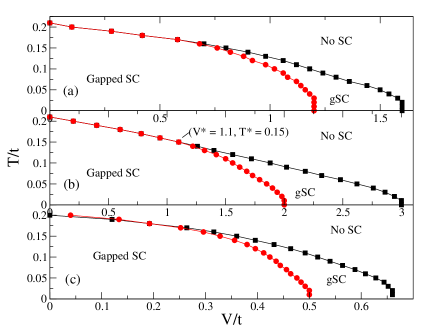
Figure 1: $V$-$T$ phase diagrams for $U=-2$, $n=0.875$ for (a) $V_{\uparrow\downarrow}$, (b) $V_{\uparrow}$, (c) $t_{\uparrow\downarrow}$. All three panels show the phase-boundaries for $\Delta_{\rm op}$ (black squares) and $E_{\rm gap}$ (red circles). Horizontal axes for the three panels are not to the same scale. ($V^{*}$, $T^{*}$) marks the critical point where the gSC phase vanishes.

In Figure 2 (a,b,c,d) we show $E_{\rm gap}$ and $\Delta_{\rm op}$ as functions of $T$ (a,b) or $V$ (c,d) for $V_{\uparrow\downarrow}$. These are the representative cuts through the $V$-$T$ diagram of Fig. 1 (a). The phase diagram, Fig. 1, is generated by sweeping disorder strength at fixed temperature, or sweeping temperature at fixed disorder. Figure 2 (a,b) shows two such vertical cuts: one at weak disorder for which there is no gapless SC phase, and one at larger disorder for which there is a gSC phase. Similarly, Figure 2 (c,d) shows horizontal cuts at fixed temperature: one at an intermediate temperature for which again there is a gSC phase, and one for a high temperature for which there is no gSC phase. Another feature to note in Figs. 2 (b,d) is that in the gSC phase $\Delta_{\rm op}$ (and $E_{\rm gap}$) is substantially reduced due to the presence of broken pairs, as noted already.

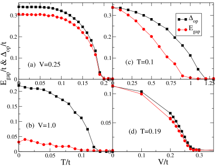
Figure 2: $E_{\rm gap}$, $\Delta_{\rm op}$ vs $T$ for (a) weak disorder $V=0.25$ showing simultaneous transitions for both $E_{\rm gap}$ and $\Delta_{\rm op}$ at $T_{c}=0.19$; (b) strong disorder $V=1$: The transition of $E_{\rm gap}$ takes place first at $T_{c}^{\rm gap}=0.1$, followed by that of $\Delta_{\rm op}$ at $T_{c}^{\rm op}=0.12$. $E_{\rm gap}$, $\Delta_{\rm op}$ vs $V$ for (c) intermediate temperature $T=0.1$, with the critical points $V_{c}^{\rm gap}=0.9$, $V_{c}^{\rm op}=1.2$; (d) high temperature $T=0.19$ with a single common critical point $V_{c}=0.27$. All panels are for the $V_{\uparrow\downarrow}$ model with $U=-2$, $n=0.875$. We identify the critical points by using the criterion that a quantity vanishes when its value becomes less than $10^{-2}$.

As a cross-check, we note that that the transition points have consistent values between Figs. 2 (a) and  2 (d), as well as between Figs. 2 (b) and  2 (c). For stronger coupling $U$, the gapless SC region at $T=0$ is larger and consequently covers larger areas of the $V$-$T$ phase plane. Its closing point moves to larger values of both ($V^{*}$, $T^{*}$).

III.2 Phase Diagram in Interaction-Disorder plane

We show the $U$-$V$ phase diagrams for $T=0$ and $n=0.875$ in Figs. 3 (a,b,c) for the three models. In the non-interacting limit ($U=0$), the entire vertical axis is an Anderson insulating phase. In the clean limit ($V=0$), the entire horizontal axis is covered by the BCS SC phase. For non-zero $U$ and $V$, we find three distinct phases: [1] The Anderson insulator bordered by $V$ axis, the origin, and a positive sloped curve passing through the origin; [2] The gapped SC phase bordered by the $|U|$ axis, origin, and a less sloped curve; and [3] the gSC phase sandwiched in between.footnote1

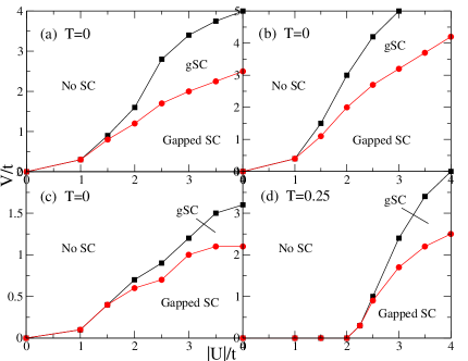
Figure 3: $U$-$V$ phase diagrams for $T=0$ (low-$T$), $n=0.875$ for (a) $V_{\uparrow\downarrow}$, (b) $V_{\uparrow}$, (c) $t_{\uparrow\downarrow}$; (d) $T=0.25$ (high-$T$), $n=0.875$ for $V_{\uparrow\downarrow}$. In (a,b,c), because of Anderson localization for arbitrarily small disorder strength and BCS pairing for arbitrarily small $|U|$, the apex of the gSC phase must actually coincide with the origin. In (d), the SC phases are destroyed for larger $|U|$ values at finite $T$. By comparing (a) and (d), we see that finite $T$ affects phase-boundaries in the weak-$V$ region of the plane more than the strong-$V$ region.

The $U$-$V$ phase diagram at finite temperature, $T=0.25$, is shown in Fig. 3 (d) for $V_{\uparrow\downarrow}$. As expected, the SC phases shrink due to thermal fluctuations. A finite $U_{c}$ is now required to get SC even in the clean limit. It also appears that while the gSC intervenes between the SC and Anderson insulator at $T=0$ when $|U|\sim 2$, there is a direct transition at finite $T$ for this interaction strength. We attribute the diminished role of disorder in giving rise to the gSC phase to the smoothing effect of thermal effects on the random potential.

III.3 Phase Diagram in Interaction-Temperature plane

We show the $U$-$T$ phase diagrams in Fig. 4 (a,b,c) for all three models at $V=0.25$ and for stronger disorder $V=2$ for the $V_{\uparrow\downarrow}$ model in Fig. 4 (d). The critical lines $T_{c}^{\rm gap}(|U|)$ and $T_{c}^{\rm op}(|U|)$ show a nearly linear increase with $|U|$, and, for weak disorder, coincide. In Fig. 4 (d), there is a gSC region for $(0<T<0.8,\,\,\,2<|U|<5)$. These results emphasize that the gSC phase is driven by the disorder $V$.

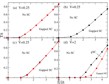
Figure 4: $U$-$T$ phase diagrams for $V=0.25$ (low-$V$), $n=0.875$ for (a) $V_{\uparrow\downarrow}$, (b) $V_{\uparrow}$, (c) $t_{\uparrow\downarrow}$; (d) $V=2$ (high-$V$), $n=0.875$ for $V_{\uparrow\downarrow}$. In (a,b,c), at low-$V$, there is no intervening gSC phase and there is a direct transition from gapped SC to insulator in the $|U|$-$T$ plane. In (d), at strong-$V$, a gSC region opens up in the $|U|$-$T$ plane.

III.4 Phase Diagram in Filling-Disorder plane

In Figs. 5 (a,b) we display the phase diagrams of the $V_{\uparrow\downarrow}$ model for $U=-2$ in the filling-disorder plane for $T=0$ (low-temperature) and $T=0.1$ (high-temperature) respectively. We restrict $n$ to the interval $0\leq n\leq 1$ because of approximate particle-hole symmetry of the potential disorder models. At $T=0$, Fig. 5 (a) shows that as the disorder strength is increased there are transitions from gapped SC to gSC to insulator for all filling values except the trivial $n=0$ case. However, at a higher temperature $T=0.1$ the SC order is destroyed for filling values below a critical filling $n_{c}=0.4$ for all $V$ (Fig. 5 (b)). For fillings greater than $n_{c}\approx 0.6$ a gSC phase appears. At low density, the effects of disorder are often larger because only the lowest energy levels, with greatest deviation from the mean, are occupied.

III.5 Phase Diagram in Filling-Temperature plane

The phase diagram in the filling-temperature plane, again for $U=-2$, is displayed in Figures 5 (c,d) for (c) low disorder, $V=0.25$, and (d) higher disorder, $V=1.0$. In Fig. 5 (c), at low disorder, there is a single line of transitions from the gapped SC phase to the insulator phase, with no intervening gSC phase. When the disorder is high, Fig. 5 (d) shows that at zero temperature, gapped SC order occurs for $n_{c}\geq 0.4$, and a gSC phase for $0.3\leq n_{c}\leq 0.4$.

At zero disorder, it is known that $T_{c}=0$ for the square lattice attractive Hubbard at half-filling ($n=1$) due to the degeneracy between superconducting and charge density correlations. It is worth noting, however, that away from half-filling the transition temperature scale is not that dramatically different from what is found in QMC and other non-MF approaches,denteneer94 ; paiva04 where $T_{c}\approx 0.1t$. It is worth noting another well-known difficulty with MF approaches, namely that the SC transition increases with $U$ at strong coupling (see Figs. 4, 5) whereas the exact $T_{c}$ turns over and falls with $1/U$.

Figure 5: (a), (b) Phase diagrams in the filling-disorder plane for interaction $U=-2$: (a) $T=0$ (low-$T$), (b) $T=0.1$ (high-$T$). (c), (d) Phase diagrams in the filling-temperature plane: (c) $V=0.25$ (low-disorder), (d) $V=1.0$ (high-disorder). At high-$T$ (b), the locations of the phase-boundaries are reduced and there exists a critical filling $n_{c}\neq 0$, compared to low-$T$ in (a). Likewise, in (c) and (d), as we go from low-$V$ to high-$V$. There is no gSC phase for low-$V$ in (c), but there is one at high-$V$ in (d). All panels are for the $V_{\uparrow\downarrow}$ model, and shown only in the interval $0\leq n\leq 1$.

IV Discussion of the Common Properties

In describing the effects of disorder, one often makes the general argument that the specific form of disorder is irrelevant to transitions, since under a renormalization flow, disorder in one term will propagate into others. This would suggest that, as we have found, the phase diagrams of our models corresponding to different types of randomness, should be qualitatively similar. However, this argument is not immediately compelling because in some cases the disorder has different symmetry properties denteneer01 . Apparently, this does not occur here. Here we make some brief observations on the quantitative differences between the phase diagrams.

For a fixed set of model parameters, particularly disorder strength, the values of $E_{\rm gap}$ and $\Delta_{\rm op}$ are higher for the $V_{\uparrow}$ site disorder than for $V_{\uparrow\downarrow}$ site disorder. Also, the values of $T_{c}$ and $V_{c}$ for destroying SC are higher for the former model compared to the latter. Similar to the $V_{\uparrow\downarrow}$ model, the $t_{\langle{\bf i}{\bf j}\rangle,\sigma}$ of the hopping disorder are uncorrelated on the same bond for different $\sigma$, so the vanishing of $E_{\rm gap}$ and $\Delta_{\rm op}$ take place at lower $T_{c}$ and $V_{c}$ as compared to $V_{\uparrow}$ model. See Figure 1 for a quantitative comparison of the how $T_{c}$ and $V_{c}$ differ between each of the three models.

A common qualitative feature of the phase diagrams is the appearance of a gSC phase. This occurs because in all these models it is possible for the low lying excited states to be located in regions where the superconducting order parameter vanishes (even though there are also significant superconducting regions). To illustrate this mechanism, first discussed in [ghosal01, ], we have correlated the regions of high or low $\Delta_{\bf i}$ with the probability of finding quasi-particles in the lowest (highest) five excited states. Here we use only a single disorder realization of the $V_{\uparrow\downarrow}$ model. Figure 6 (a) shows significant overlap between $\Delta_{\bf i}$ and the highest probability for quasi-particle/hole excitations in the ten states, while Figure 6 (b) shows the non-overlap of these regions. This leads to finite $T$ gapped and gSC excitations respectively.

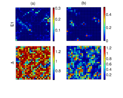
Figure 6: Real-space plots for the $V_{\uparrow\downarrow}$ model. Left panels (a): Sum of wave-function amplitude-squared for the first five excited states above and below ‘$\mu$’ and $\Delta_{\bf i}$ at $T=0.4$ for $U=-4$, $V=0.5$ (in the gapped SC phase). These show the overlap of the weight of the single-particle low-energy excitations with regions of significant SC order. Right panels (b): The same for $U=-4$, $V=2.0$ (gSC phase), which show the non-overlap of the low-energy states with the SC islands, leading to the gapless SC phase.

The presence of a uniform Zeeman field on a clean (disordered) attractive Hubbard lattice is known to induce a spin-imbalance and resulting FFLO (dLO) phases with sign-changing energy gap $\Delta_{\bf i}$ within BdG MFTcui08 . Since we have random Zeeman fields in two of our models (and hence local spin-imbalance), it is natural to ask whether sign changes in $\Delta_{\bf i}$ occur. We find that our models do not have a sign changing $\Delta_{\bf i}$, and, in fact, that such sign changes are a diagnostic that we have converged to an incorrect, metastable solution.

This result is consistent with a recent BdG study of a 1D balanced system $N_{\uparrow}=N_{\downarrow}$ which similarly found no sign-changes in $\Delta_{\bf i}$ in the presence of a single magnetic impurity, despite the presence of local spin-imbalance and a reduced value of $\Delta_{\bf i}$ at and around the defect ljiang11 . On the other hand, in the same study, the authors also find that a sufficiently extended magnetic impurity in 1D and 3D, for example, with a Gaussian profile, does result in both a local spin-imbalance and sign-changes in $\Delta_{\bf i}$ (FFLO phase). Similarly, another recent BdG studyzapata10 in 1D with $N_{\uparrow}=N_{\downarrow}$ and a spin-dependent lattice [$V_{\uparrow}(x)=-V_{\downarrow}(x)=V_{0}{\rm cos}(2\pi x/\lambda)$] concluded that “$\pi$ phases” which exhibit sign-changing $\Delta_{\bf i}$ require spin-dependent lattices with wave-length longer than the coherence length.

Thus the absence of sign-changing $\Delta_{\bf i}$ in our work is due to our choice of spatially uncorrelated random magnetic impurities at every site and consequently a spin-dependent lattice potential with wavelength much less than the coherence length. Current experiments can introduce such very rapidly varying laser speckle aspect09 ; palencia10 .

V Special Cases of the Models

To understand better the physics of spin-dependent disorder within the 2D attractive Hubbard model, we explored some particular features of the $V_{\uparrow\downarrow}$ model.

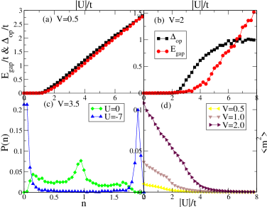
Figure 7: For the $V_{\uparrow\downarrow}$ model, $E_{\rm gap}$, $\Delta_{\rm op}$ vs $|U|$ for (a) $V=0.5$: $E_{\rm gap}$ and $\Delta_{\rm op}$ increase without bound at low disorder; (b) $V=2.0$: at high disorder, $E_{\rm gap}$ increases without bound while $\Delta_{\rm op}$ saturates. (c) The particle distribution $P(n)$ for $V=3.5$, $U=0$: There is roughly a three-peak structure implying that most sites are empty, singly-, or doubly-occupied for spin-dependent disorder at weak interactions. For the same $V$ and $U=-7$, the peak near $n\approx 1$ has disappeared, so single occupancy is disfavored for $|U|\gg V$. (d) The local-moment $\langle m^{2}\rangle$ vs $|U|$ for $V=0.5$, 1.0, 2.0: As $V$ becomes stronger, the initial local-moment is higher. However, as $|U|$ is increased, the local-moment is driven to zero in the regime $|U|\gg V$. All panels for $T=0$, $n=0.875$.

In Figure 7 (c) we show the particle density histogram for $|U|=0,7$. For $|U|=0$, we find the disorder landscape favors site fillings of approximately zero, one, or two particles. For $|U|=7$, we see that the histogram has only two peaks at fillings of zero and two. This can also be seen in Figures 7 (a,b). Fig. 7 (a), for $V=0.5$, shows $E_{\rm gap}$ and $\Delta_{\rm op}$ increase without bound versus $|U|$ and $\Delta_{\rm op}\geq E_{\rm gap}$, as is always the case for spin-dependent disorder; but in Fig. 7 (b), for $V=2.0$ and for strong enough $|U|\gg V$, we find that $\Delta_{\rm op}\leq E_{\rm gap}$ and saturates. In previous spin-independent BdG work in Ref. ghosal01, ; ghosal98, , it was found that $\Delta_{\rm op}\leq E_{\rm gap}$ for all disorder strengths. Here we find that we recover some of the results of the spin-independent disorder for $|U|\gg V$.

In Fig. 7 (d) we show the evolution of the site-averaged, squared local-moment, $\langle m^{2}\rangle$, as a function of $|U|$ for three disorder strengths, $V=0.5,1.0,2.0$ at $T=0$. When $|U|=0$, the moment starts out at its maximum possible value. This maximum value is larger for greater $V$ because the potential minima for the $\uparrow$-fermions and $\downarrow$-fermions are in general at different sites due to the spin-dependent randomness. As $|U|$ increases, it becomes energetically favorable for two fermions of opposite spin to occupy the same site forming a singlet, and as a result, decreasing the local moment all the way to zero for very large $|U|$.

The destruction of the average local-moment is seen to occur at roughly the same $|U|$ value where the cross-over from $\Delta_{\rm op}>E_{\rm gap}$ to $\Delta_{\rm op}<E_{\rm gap}$ takes place in Fig. 7 (b). Spin-independent disorder always has the property $\langle m^{2}\rangle=0$, since both spin-species see the same potential landscape. The average local-moment destruction for large $|U|$ is, therefore, also an indication that in the $|U|\gg V$ limit, we are in the spin-independent regime.

VI Conclusions

Before summarizing the results of this paper, we relate our study to previous classic investigations of magnetic impurities in superconductors. One of the earliest works on this topic was by Abrikosov and Gor’kov (AG)ag61 who considered a continuum model of a weak-coupling superconductor with dilute magnetic impurities in the form of randomly distributed and oriented classical spins coupled to the electrons via a rotationally invariant exchange interaction. As with our Zeeman interaction, this external magnetic field breaks time-reversal invariance and suppresses superconductivity since it is not protected by Anderson’s Theorem anderson59 . AG’s mean field treatment uses the perturbative, self-consistent, Born approximation. Although the magnetic disorder results in an inhomogeneous $\Delta_{\bf i}$, due to the diluteness of the impurities, $\Delta_{\bf i}$ is rather different from that considered here. It is predominantly spatially uniform except in the vicinity of the impurity moments. In fact, although their formalism admits inhomogeneity, in solving the resulting integral equation the order parameter is assumed constant. AG find that the quasiparticle energies and $\Delta_{\rm op}$ are modified in different ways and, as a consequence $E_{\rm gap}$ is suppressed more than $\Delta_{\rm op}$. The more rapid decay of $E_{\rm gap}$ leads to a gapless SC phase, as found here.

To check the validity of AG theory in the strong disorder regime, we modified our BdG codes to enforce a spatially uniform $\Delta_{\bf i}$ equal to the site average of the inhomogeneous $\Delta_{\bf i}$. We found that the region of gapless SC phase is greatly diminished compared to the case of inhomogeneous $\Delta_{\bf i}$ jiang11 . This illustrates the limitations of AG theory in addressing the physics of strong disorder, and it also validates our physical picture for the gapless SC phase. A nearly uniform $\Delta_{\bf i}$ precludes the possibility of a mechanism for the gapless SC phase based on our physical picture (see below).

Like AG, our work is at the mean-field level. However, since it is based on the non-perturbative BdG MFT, it can capture strong coupling effects, as well as strong inhomogeneities in $\Delta_{\bf i}$ which occur throughout the lattice and not just on widely separated impurity sites. As described earlier, these effects lead to a clear physical picture for the gapless SC phase namely, that the lowest lying quasi-particle/hole excited states lie in the Anderson insulator regions where there is no SC order, and hence a zero excitation gap. Such an interpretation is absent from AG theory. A further distinct feature of our work, as compared to the AG treatment, is that the non-interacting eigenstates are Anderson localized (in regions which are different for the up and down spins) so our ‘normal’ state is a (spin-dependent) Anderson Insulator, whereas the normal state of the AG model is band metallic.

In this paper we have explored the interplay of strong attractive interactions and spin-dependent disorder with rapid spatial variation. We have mapped out the ground state phase diagrams for various cases- when one species moves in an environment completely decoupled from the disorder, when both species see randomness, but the energy landscape is species dependent, and finally when the hopping is random, but dependent on the fermion spin. We find that, as the disorder is increased, in some situations the superconducting gap goes to zero first, followed by the order parameter. That is, there can be a gapless superconducting phase.

Our numerical results are for systems of finite size, most typically 24$\times$24 lattices. Some finite size scaling was used, for example to demonstrate small residual values of $E_{\rm gap}$ scale to zero with increasing system size. We should mention, however, that on these finite lattices it is difficult to access any physics associated with rare regions, e.g. an exponential ‘tail’ density-of-states which starts from the gap edge ($E_{\rm gap}$) at a maximum and extends to $E=0$, the so-called “soft gap” balatsky97 ; lamacraft00 ; lamacraft01 ; balatskyRMP06 .

We have considered the phase diagram/equilibrium thermodynamics here, but transport properties pose some interesting questions. For example, when $U=0$ and one spin species sees no disorder, it will be metallic while the other is insulating. As the attractive $U$ is turned on, the metallic species will see an induced randomness. At $U$ nonzero will both species be localized or extended, or can there be parameter regimes where there is a ‘spin selective Anderson transition’?

Mean field approaches such as the BdG treatment used here are, of course, only approximate, and are problematic at finite temperatures since they ignore phase fluctuations. Studies of the attractive Hubbard model with Quantum Monte Carlo methods offer a way to treat the interactions exactly, although on lattices of smaller size than with the BdG approach described here. Quantum Monte Carlo can go to very low temperatures and access the superconducting phase, if it exists, because there is no sign problem either in the clean case scalettar89 ; moreo91 ; imada91 ; assaad94 or for randomness which is the same for both spin species huscroft97 ; hurt05 . Unfortunately, spin-dependent disorder will introduce a sign problem loh90 in determinant Quantum Monte Carlo even for the case of attractive interactions. Indeed, once one allows for both a non-zero chemical potential and a non-zero Zeeman field, the positive and negative $U$ Hubbard models can be mapped onto each other exactly. Thus we expect limited ability to address the physics of spin dependent disorder with this method. Studies via dynamical mean field theory, on the other hand are feasible at low temperature, and would offer a more precise theoretical point of contact than the present mean field treatment with optical lattice experiments when they are performed.

VII Acknowledgements

This work was supported by the Department of Energy under DE-FG52-09NA29464; by the National Science Foundation under grants PHY-1005503 and PHY-1004848 and by the CNRS-UC Davis EPOCAL LIA joint research grant.

References

- (1) P. A. Lee and T. V. Ramakrishnan, Rev. Mod. Phys. 57, 287 (1985).
- (2) D. Belitz and T. R. Kirkpatrick, Rev. Mod. Phys. 66, 261 (1994).
- (3) E. Abrahams, P.W. Anderson, D.C. Licciardello, and T.V. Ramakrishnan, Phys. Rev. Lett. 42, 673 (1979).
- (4) S.V. Kravchenko, G.V. Kravchenko, J.E. Furneaux, V.M. Pudalov, and M. D’Iorio, Phys. Rev. B50, 8039 (1994); S.V. Kravchenko, D. Simonian, M. P. Sarachik, W. Mason, and J. E. Furneaux, Phys. Rev. Lett. 77, 4938 (1996).
- (5) D. Popovic, A. B. Fowler, and S. Washburn, Phys. Rev. Lett. 79, 1543 (1997).
- (6) E. Abrahams, S. V. Kravchenko, and M. P. Sarachik, Rev. Mod. Phys. 73, 251 (2001).
- (7) A.E. White, R.C. Dynes, and J.P. Garno, Phys. Rev. B33, 3549 (1986).
- (8) B.G. Orr, H.M. Jaeger, A.M. Goldman and C.G. Kuper, Phys. Rev. Lett. 56, 378 (1986).
- (9) M.P.A. Fisher, G. Grinstein and S.M. Girvin, Phys. Rev. Lett. 64, 587 (1990).
- (10) A. F. Hebard, in “Strongly Correlated Electronic Systems” edited by K. S. Bedell, Z. Wang, D. E. Meltzer, A. V. Balatsky, and E. Abrahams, (Addison-Wesley, 1994), and references cited therein.
- (11) D. Jaksch, C. Bruder, J.I. Cirac, C.W. Gardiner, and P. Zoller, Phys. Rev. Lett. 81, 3108 (1998).
- (12) I. Bloch, J. Dalibard, and W. Zwerger, Rev. Mod. Phys. 80, 885 (2005).
- (13) A. Aspect and M. Inguscio, Physics Today 62, 30 (2009).
- (14) L. S.-Palencia and M. Lewenstein, Nature Phys. 6, 87 (2010).
- (15) C. Chin, R. Grimm, P. Julienne and E. Tiesinga, Rev. Mod. Phys. 82, 1225 (2010).
- (16) M. White, M. Pasienski, D. McKay, S.Q. Zhou, D. Ceperley, and B. DeMarco, Phys. Rev. Lett. 102, 055301 (2009).
- (17) S. Q. Zhou and D. M. Ceperley, Phys. Rev. A81, 013402 (2010).
- (18) B. De Marco, private communication.
- (19) D. McKay and B. DeMarco, New Journal of Physics 12, 055013 (2010).
- (20) O. Mandel, M. Greiner, A. Widera, T. Rom, T.W. Hänsch, and I. Bloch, Nature 425, 937 (2003); Phys. Rev. Lett. 91, 010407 (2003).
- (21) A.E. Feiguin and M.P.A. Fisher, Phys. Rev. Lett. 103, 025303 (2009).
- (22) W.V. Liu, F. Wilczek, and P. Zoller, Phys. Rev. A70, 033603 (2004).
- (23) P.G. de Gennes, Superconductivity in Metals and Alloys, Benjamin, New York (1966).
- (24) P. W. Anderson, J. Phys. Chem. Solids 11, 26 (1959).
- (25) M. Jiang, R. Nanguneri, N. Trivedi, G.G. Batrouni, R.T. Scalettar, cond-mat/1109.1622.
- (26) M. Pasienski, D. McKay, M. White and B. DeMarco, Nat. Phys. 6, 677 (2010).
- (27) M. Pasienski, Ph.D. thesis, (2011).
- (28) S.S. Kondov, W.R. McGehee, J.J. Zirbel, and B. De Marco, cond-mat/1105.5368.
- (29) M. Pasienski, private communication.
- (30) S. Robaszkiewicz, R. Micnas, and K.A. Chao, Phys. Rev. 23, 1447 (1981).
- (31) R.T. Scalettar, E.Y. Loh, Jr., J.E. Gubernatis, A. Moreo, S.R. White, D.J. Scalapino, R.L. Sugar, and E. Dagotto, Phys. Rev. Lett. 62, 1407 (1989).
- (32) P.J.H. Denteneer, Phys. Rev. B49, 6364 (1994).
- (33) R.R. dos Santos, Phys. Rev. B50, 635 (1994).
- (34) T. Paiva, R.R. dos Santos, R.T. Scalettar, and P.J.H. Denteneer, Phys. Rev. B69, 184501 (2004).
- (35) K. Aryanpour, E.R. Dagotto, M. Mayr, T. Paiva, W.E. Pickett, and R.T. Scalettar, Phys. Rev. B73, 104518 (2006).
- (36) In some situations, in the thermodynamic limit, unbounded disorder can produce somewhat different effects from bounded disorder.
- (37) A. Ghosal, M. Randeria, and N. Trivedi, Phys. Rev. Lett. 81, 3940 (1998).
- (38) A. Ghosal, M. Randeria, and N. Trivedi, Phys. Rev. B65, 014501 (2001).
- (39) P. Fulde and A. Ferrell, Phys. Rev. 135, A550 (1964).
- (40) A. Larkin and Y.N. Ovchinnikov, Zh. Eksp. Teor. Fiz. 47, 1136 (1964) [Sov. Phys. JETP 20, 762 (1965)].
- (41) P.J.H. Denteneer, R.T. Scalettar, and N. Trivedi, Phys. Rev. Lett. 87, 146401 (2001).
- (42) We note that in MF calculations in the clean limit at , finite lattice effects obscure the BCS phase at small . Simulation of larger lattices is required to get the precise boundaries in the region of Figure 3.
- (43) Q. Cui and K. Yang, Phys. Rev. B78, 054501 (2008).
- (44) L. Jiang, L. O. Baksmaty, H. Hu, Y. Chen, and H. Pu, Phys. Rev. A83, 061604(R) (2011).
- (45) I. Zapata, B. Wunsch, N. T. Zinner, and E. Demler, Phys. Rev. Lett. 105, 095301 (2010).
- (46) A. A. Abrikosov and L. P. Gor’kov, Sov. Phys. JETP 12, 1243 (1961).
- (47) A. V. Balatsky and S. A. Trugman, Phys. Rev. Lett. 79, 3767 (1997).
- (48) A. Lamacraft and B. D. Simons, Phys. Rev. Lett. 85, 4783 (2000).
- (49) A. Lamacraft and B. D. Simons, Phys. Rev. B, 64, 014514 (2001).
- (50) A. V. Balatsky, I. Vekhter, Jian-Xin Zhu, Rev. Mod. Phys. 78, 373 (2006).
- (51) A. Moreo and D.J. Scalapino, Phys. Rev. Lett. 66, 946 (1991).
- (52) M. Imada, Physica C185-189, 1447 (1991).
- (53) F.F. Assaad, W. Hanke, and D.J. Scalapino, Phys. Rev. B49, 4327 (1994).
- (54) C. Huscroft and R.T. Scalettar, Phys. Rev. B55, 1185 (1997).
- (55) D. Hurt, E. Odabashian, W.E. Pickett, R.T. Scalettar, F. Mondaini, T. Paiva, and R. dos Santos, Phys. Rev B72, 144513 (2005).
- (56) E.Y. Loh, J.E. Gubernatis, R.T. Scalettar, S.R. White, D.J. Scalapino, and R.L. Sugar, Phys. Rev. B41, 9301 (1990).