Notes on a new construction of hyperkähler metrics

1 Overview

In joint work with Davide Gaiotto and Greg Moore [1] we recently proposed a new connection between hyperkähler geometry and the counting of BPS states in supersymmetric field theory. While the story is motivated by physics, it leads to a concrete new recipe for constructing complete hyperkähler metrics on the total spaces of certain complex integrable systems.

The aim of this note is briefly to describe what this recipe is, and to comment on some of the issues involved in converting it into an actual theorem.

Let us briefly describe some of the highlights.

• We begin with a collection of “integrable system data” described in Section 2.1 below. These data include a complex manifold $\mathcal{B}$ containing a divisor $D$. For example, $\mathcal{B}$ could be the complex plane, and $D$ some collection of points. The data also include a local system of lattices $\Gamma$ over $\mathcal{B}^{\prime}=\mathcal{B}\setminus D$, from which we build a $2r$-torus bundle $\mathcal{M}^{\prime}$ over $\mathcal{B}^{\prime}$, with nontrivial monodromy around $D$. Finally, we have a “central charge” homomorphism $Z:\Gamma\to\mathbb{C}$, varying holomorphically over $\mathcal{B}^{\prime}$. From these data we build a simple explicit hyperkähler metric $g^{\mathrm{sf}}$ on $\mathcal{M}^{\prime}$. However, the metric $g^{\mathrm{sf}}$ is incomplete, and our main interest is in complete metrics.

• Naively we might hope to complete $g^{\mathrm{sf}}$ by adding some degenerate torus fibers over $D$, thus extending $\mathcal{M}^{\prime}$ to $\mathcal{M}\supset\mathcal{M}^{\prime}$, in such a way that $g^{\mathrm{sf}}$ will extend to $\mathcal{M}$. However, it seems that this is impossible: roughly speaking, $g^{\mathrm{sf}}$ is too homogeneous to have such an extension. Instead, we construct a new metric $g$ on $\mathcal{M}^{\prime}$, which differs from $g^{\mathrm{sf}}$ by certain “quantum corrections.”

• The quantum corrections are obtained by solving a certain explicit integral equation, (4.8) below. The main new ingredient in this equation is a set of integer “invariants” $\Omega(\gamma)$, which should be examples of generalized Donaldson-Thomas invariants in the sense of [2, 3]. In particular, the Kontsevich-Soibelman wall-crossing formula for generalized Donaldson-Thomas invariants, as written in [2], plays an important role in the construction. Indeed the original motivation for this construction was an attempt to understand the physical meaning of the formula of [2].

• Both the metrics $g^{\mathrm{sf}}$ and $g$ depend on a real parameter $R>0$; in the limit as $R\to\infty$, the torus fibers of $\mathcal{M}^{\prime}$ collapse, in either metric. The corrections $g-g^{\mathrm{sf}}$ are exponentially suppressed in $R$ when we are away from $D$: so as $R\to\infty$, $g$ looks very close to $g^{\mathrm{sf}}$ except in a small neighborhood of the singular fibers. Near the singular fibers the quantum corrections become large, and in particular we expect that the corrected $g$ can be extended over the singular fibers.

  This description of $g$ near the $R\to\infty$ limit should be thought of as an example of a more general picture of the geometry of Calabi-Yau manifolds near their large complex structure limit, proposed by Gross-Wilson [4], Kontsevich-Soibelman [5] and Todorov, motivated by the Strominger-Yau-Zaslow picture of mirror symmetry [6].

• In many examples where our recipe can be applied, it turns out that the hyperkähler metrics in question were already known to exist. The example we have studied in most detail is that of rank-2 Hitchin systems with semisimple ramification [7]. We briefly describe that example in Section 9 below.

• Our recipe has not really been tested so far, in the sense that nobody has tried hard to use it to get new explicit information about interesting hyperkähler metrics. We believe that this should be possible: at the very least it should be possible to get a precise asymptotic series for $g$ as $R\to\infty$.

I thank Cesar Garza, Tom Sutherland, and the anonymous referee for very useful comments and for correcting several errors in an earlier draft of this note. I would also like to thank Davide Gaiotto and Greg Moore for a very enjoyable collaboration.

This work is supported by National Science Foundation grants DMS-1160461 and DMS-1151693.

2 Integrable system data

2.1 Data

Our construction begins with the following data:

• A complex manifold $\mathcal{B}$, of dimension $r$ (“Coulomb branch”).

• A divisor $D\subset\mathcal{B}$ (“discriminant locus”). Let $\mathcal{B}^{\prime}=\mathcal{B}\setminus D$ (“smooth locus”). We use $u$ to denote a general point of $\mathcal{B}^{\prime}$.

• A local system $\Gamma_{\mathrm{g}}$ over $\mathcal{B}^{\prime}$, with fiber a rank-$2r$ lattice, equipped with a nondegenerate antisymmetric integer-valued pairing $\langle,\rangle$. Abusing notation we will also use $\langle,\rangle$ to denote the inverse pairing on $\Gamma_{\mathrm{g}}^{*}$ (not necessarily integer-valued.) Data 3b: A fixed lattice $\Gamma_{\mathrm{f}}$ (possibly trivial). We sometimes think of $\Gamma_{\mathrm{f}}$ as the fiber of a trivial local system of lattices over $\mathcal{B}^{\prime}$. Data 3c: A local system $\Gamma$ of lattices over $\mathcal{B}^{\prime}$, given as an extension $$0\to\Gamma_{\mathrm{f}}\to\Gamma\to\Gamma_{\mathrm{g}}\to 0.$$ (2.1) The pairing $\langle,\rangle$ on $\Gamma_{\mathrm{g}}$ induces one on $\Gamma$ which we also denote $\langle,\rangle$. The radical of this pairing is $\Gamma_{\mathrm{f}}$.

• A homomorphism $Z:\Gamma\to\mathbb{C}$, varying holomorphically over $\mathcal{B}^{\prime}$. For any local section $\gamma$ of $\Gamma$ we thus get a local holomorphic function $Z_{\gamma}$ on $\mathcal{B}^{\prime}$.

• A homomorphism $\theta_{\mathrm{f}}:\Gamma_{\mathrm{f}}\to\mathbb{R}/2\pi\mathbb{Z}$.

These data are subject to several conditions:

• $Z_{\gamma_{f}}$ is a constant function on $\mathcal{B}^{\prime}$ for any $\gamma_{f}\in\Gamma_{\mathrm{f}}$. (As a consequence, the $\Gamma^{*}$-valued 1-form $\mathrm{d}Z$ actually descends to $\Gamma_{\mathrm{g}}^{*}$; we use this in formulating Condition 2.)

• $\langle\mathrm{d}Z\wedge\mathrm{d}Z\rangle=0$.

• For any $u\in\mathcal{B}^{\prime}$, the $\mathrm{d}Z_{\gamma}(u)$ span $\mathcal{T}^{*}_{u}\mathcal{B}^{\prime}$.

2.2 Integrable system

The above data are enough to determine an incomplete complex integrable system, i.e. a holomorphic symplectic manifold $\mathcal{M}^{\prime}$ which is a fibration over a complex base manifold $\mathcal{B}^{\prime}$, with fibers complex Lagrangian tori. We now describe $\mathcal{M}^{\prime}$.

For any fiber $\Gamma_{u}$ of $\Gamma$, let $\operatorname{TChar}_{u}(\Gamma,\theta_{\mathrm{f}})$ be the set of twisted unitary characters of $\Gamma_{u}$, i.e. maps $\theta:\Gamma_{u}\to\mathbb{R}/2\pi\mathbb{Z}$ obeying

$$\theta_{\gamma}+\theta_{\gamma^{\prime}}=\theta_{\gamma+\gamma^{\prime}}+\pi\langle\gamma,\gamma^{\prime}\rangle,$$ (2.2)

agreeing with $\theta_{\mathrm{f}}$ when restricted to $\Gamma_{\mathrm{f}}\subset\Gamma_{u}$. $\operatorname{TChar}_{u}(\Gamma,\theta_{\mathrm{f}})$ is topologically a torus $(S^{1})^{2r}$. Letting $u$ vary, the $\operatorname{TChar}_{u}(\Gamma,\theta_{\mathrm{f}})$ are the fibers of a torus bundle $\mathcal{M}^{\prime}$ over $\mathcal{B}^{\prime}$. Any local section $\gamma$ of $\Gamma$ then gives a function “evaluation on $\gamma$,”

$$\theta_{\gamma}:\mathcal{M}^{\prime}\to\mathbb{R}/2\pi\mathbb{Z}.$$ (2.3)

These are the angular coordinates on the torus fibers of $\mathcal{M}^{\prime}$.

Now we want to construct the complex structure and holomorphic symplectic form on $\mathcal{M}^{\prime}$. For this purpose note that we have canonical functions

$$Z_{\gamma}:\mathcal{M}^{\prime}\to\mathbb{C},$$ (2.4)

pulled back from the base $\mathcal{B}^{\prime}$. Differentiating gives a collection of 1-forms $\mathrm{d}\theta_{\gamma}$ and $\mathrm{d}Z_{\gamma}$ on $\mathcal{M}^{\prime}$, which are linear in $\gamma$ and vanish for $\gamma\in\Gamma_{\mathrm{f}}$, and hence can be organized into $\Gamma_{\mathrm{g}}^{*}$-valued 1-forms $\mathrm{d}\theta$ and $\mathrm{d}Z$. Then define the complex 2-form

$$\omega_{+}=-\frac{1}{2\pi}\langle\mathrm{d}Z\wedge\mathrm{d}\theta\rangle.$$ (2.5)

There is a unique complex structure on $\mathcal{M}^{\prime}$ for which $\omega_{+}$ is of type $(2,0)$. We call this complex structure $J(\zeta=0)$, for a reason which will emerge momentarily.

The two-form $\omega_{+}$ gives a holomorphic symplectic structure on $(\mathcal{M}^{\prime},J(\zeta=0))$. With respect to this structure, the projection $\pi:\mathcal{M}^{\prime}\to\mathcal{B}^{\prime}$ is holomorphic, and the torus fibers $\mathcal{M}^{\prime}_{u}=\pi^{-1}(u)$ are compact complex Lagrangian submanifolds.

2.3 Affine structures

Although we do not use it explicitly in the rest of this note, it may be useful to mention that our data determine an $S^{1}$ worth of (symplectic) affine structures on $\mathcal{B}^{\prime}$. Fix some $\vartheta\in\mathbb{R}/2\pi\mathbb{Z}$. Then pick a patch $U\subset\mathcal{B}^{\prime}$ on which $\Gamma_{\mathrm{g}}$ admits a basis of local sections, $\gamma_{1},\dots,\gamma_{2r}$, in which $\langle,\rangle$ is the standard symplectic pairing. Also choose a local splitting $\rho:\Gamma_{\mathrm{g}}\to\Gamma$ of (2.1). Then the functions

$$f_{i}=\operatorname{Re}(e^{{\mathrm{i}}\vartheta}Z_{\rho(\gamma_{i})})$$ (2.6)

are local coordinates on $U$ (possibly after shrinking $U$). The transition functions on overlaps $U\cap U^{\prime}$ are valued in $\operatorname{Sp}(2r,\mathbb{Z})\ltimes\mathbb{R}^{2r}$ (the $\operatorname{Sp}(2r,\mathbb{Z})$ part comes from the choice of basis of $\Gamma_{\mathrm{g}}$, the $\mathbb{R}^{2r}$ from the choice of splitting $\rho$.)

3 Semiflat hyperkähler metric

We now impose one more condition. Recall that a positive 2-form $\omega$ on a complex manifold is a real 2-form for which $\omega(v,Jv)>0$ for all real tangent vectors $v$.

• $\langle\mathrm{d}Z\wedge\mathrm{d}\bar{Z}\rangle$ is a positive 2-form on $\mathcal{B}^{\prime}$.

3.1 Semiflat metric

Fix $R\in\mathbb{R}_{+}$. $\mathcal{M}^{\prime}$ carries a canonical 2-form,

$$\omega_{3}^{\mathrm{sf}}=\frac{R}{4}\langle\mathrm{d}Z\wedge\mathrm{d}\bar{Z}\rangle-\frac{1}{8\pi^{2}R}\langle\mathrm{d}\theta\wedge\mathrm{d}\theta\rangle.$$ (3.1)

This form is of type $(1,1)$ in complex structure $J(\zeta=0)$ and positive. So the triple $(\mathcal{M}^{\prime},J(\zeta=0),\omega_{3}^{\mathrm{sf}})$ determine a Kähler metric $g^{\mathrm{sf}}$ on $\mathcal{M}^{\prime}$. In fact this metric is hyperkähler. As far as I know, the first place where this was shown is in [8] (albeit in somewhat different notation); see also [9] for a more modern account. Alternatively, though, the hyperkähler property is a consequence of the twistorial construction of the metric which we will give below.

The superscript ^sf stands for “semi-flat”: this terminology first appeared in [4], where it was used to refer to an important special case introduced in [10]. The reason for the name is that $g^{\mathrm{sf}}$ is flat when restricted to any torus fiber $\mathcal{M}^{\prime}_{u}$, and $\mathcal{M}^{\prime}_{u}$ has half the dimension of $\mathcal{M}^{\prime}$.

3.2 Twistorial description of the semiflat metric

Let us now describe a different, “twistorial” way of constructing the metric $g^{\mathrm{sf}}$; this alternative description is what we will generalize in our construction of the quantum-corrected metric $g$ below.

Any hyperkähler metric on a manifold $\mathcal{M}^{\prime}$ determines — and is determined by — a collection of holomorphic symplectic structures $(\mathcal{M}^{\prime},J(\zeta),\varpi(\zeta))$ labeled by $\zeta\in\mathbb{C}\mathbb{P}^{1}$. In the general theory of hyperkähler manifolds all $\zeta$ are on the same footing. However, for the hyperkähler manifolds we are describing in this note, the points $\zeta=0$ and $\zeta=\infty$ will play a distinguished role. It is then convenient to expand $\varpi(\zeta)$ as

$$\varpi(\zeta)=-\frac{i}{2\zeta}\omega_{+}+\omega_{3}-\frac{i}{2}\zeta\overline{\omega_{+}}$$ (3.2)

where $\omega_{+}$, $\omega_{3}$ are respectively the holomorphic symplectic form and Kähler form, both relative to the complex structure $J(\zeta=0)$.

In the particular case of the hyperkähler metric $g^{\mathrm{sf}}$, we have written these 2-forms explicitly above in (2.5), (3.1). We will now give an alternative description of the holomorphic symplectic forms $\varpi(\zeta)$ corresponding to $g^{\mathrm{sf}}$, roughly by exhibiting explicit holomorphic Darboux coordinates.

Let $T_{u}$ denote the complex torus of twisted complex characters of $\Gamma_{u}$. $T_{u}$ has canonical $\mathbb{C}^{\times}$-valued functions $X_{\gamma}$ ($\gamma\in\Gamma_{u}$) obeying

$$X_{\gamma}X_{\gamma^{\prime}}=(-1)^{\langle\gamma,\gamma^{\prime}\rangle}X_{\gamma+\gamma^{\prime}},$$ (3.3)

and a Poisson structure

$$\{X_{\gamma},X_{\gamma^{\prime}}\}=\langle\gamma,\gamma^{\prime}\rangle X_{\gamma+\gamma^{\prime}}.$$ (3.4)

The $T_{u}$ glue together into a local system over $\mathcal{B}^{\prime}$ with fiber a complex Poisson torus. Let $T$ denote the pullback of this local system to $\mathcal{M}^{\prime}$.

Now we consider a section $\mathcal{X}^{\mathrm{sf}}$ of $T$, depending on an auxiliary parameter $\zeta\in\mathbb{C}^{\times}$. Locally this just means a collection of “coordinate” functions

$$\mathcal{X}^{\mathrm{sf}}_{\gamma}:\mathcal{M}^{\prime}\times\mathbb{C}^{\times}\to\mathbb{C}^{\times}$$ (3.5)

(defined by $\mathcal{X}^{\mathrm{sf}}_{\gamma}=(\mathcal{X}^{\mathrm{sf}})^{*}X_{\gamma}$, with $\gamma$ a local section of $\Gamma$). We often write these functions as $\mathcal{X}^{\mathrm{sf}}_{\gamma}(\zeta)$, leaving the $\mathcal{M}^{\prime}$ dependence implicit. $\mathcal{X}^{\mathrm{sf}}(\zeta)$ is given by a simple closed formula:

$$\mathcal{X}^{\mathrm{sf}}_{\gamma}(\zeta)=\exp\left[\pi R\frac{Z_{\gamma}}{\zeta}+{\mathrm{i}}\theta_{\gamma}+\pi R\zeta\bar{Z}_{\gamma}\right].$$ (3.6)

Now a direct computation shows

$$\varpi^{\mathrm{sf}}(\zeta)=\frac{1}{8\pi^{2}R}\langle\mathrm{d}\log\mathcal{X}^{\mathrm{sf}}(\zeta)\wedge\mathrm{d}\log\mathcal{X}^{\mathrm{sf}}(\zeta)\rangle.$$ (3.7)

So the $\mathcal{X}^{\mathrm{sf}}_{\gamma}(\zeta)$ are “holomorphic Darboux coordinates” on $\mathcal{M}^{\prime}$, determining the holomorphic symplectic structures for all $\zeta\in\mathbb{C}^{\times}$, and hence the hyperkähler metric $g^{\mathrm{sf}}$. In short: knowing the functions $\mathcal{X}^{\mathrm{sf}}_{\gamma}(\zeta)$ is equivalent to knowing the hyperkähler metric $g^{\mathrm{sf}}$.

A global way of thinking about this construction is to say that for each $\zeta\in\mathbb{C}^{\times}$ we pull back the structure of holomorphic Poisson manifold from $T$ to $\mathcal{M}^{\prime}$, using the section $\mathcal{X}^{\mathrm{sf}}(\zeta)$ of $T$. After pullback the Poisson structure is actually nondegenerate, i.e. it arises from a holomorphic symplectic structure.

4 Instanton corrections to $\mathcal{X}$

We explained above how the semiflat section $\mathcal{X}^{\mathrm{sf}}$ can be used to construct the holomorphic-symplectic forms $\varpi(\zeta)$ corresponding to the semiflat metric $g^{\mathrm{sf}}$. We now want to construct a new, “quantum-corrected” section $\mathcal{X}$. In the next section we will use $\mathcal{X}$ to build a quantum-corrected metric $g$.

4.1 BPS degeneracies and Riemann-Hilbert problem

The key new ingredient determining the quantum corrections is:

• A function $\Omega:\Gamma\to\mathbb{Z}$.

For each local section $\gamma$ of $\Gamma$ this gives a locally defined integer-valued function $\Omega(\gamma)$ on $\mathcal{B}^{\prime}$. I emphasize that $\Omega$ is not required to be continuous: indeed Condition 7 below will imply that it is generally not continuous, but jumps in a specific way (governed by the Kontsevich-Soibelman wall-crossing formula) at real-codimension-1 loci in $\mathcal{B}^{\prime}$.

$\Omega$ should obey a simple parity-invariance condition:

$\Omega(\gamma;u)=\Omega(-\gamma;u)$.

We can now formulate the key ingredient in our construction, a certain Riemann-Hilbert problem. We need a little notation. Any $\gamma\in\Gamma_{u}$ gives a birational Poisson automorphism $\mathcal{K}_{\gamma}$ of $T_{u}$, defined by

$$\mathcal{K}_{\gamma}^{*}X_{\gamma^{\prime}}=X_{\gamma^{\prime}}(1-X_{\gamma})^{\langle\gamma,\gamma^{\prime}\rangle}.$$ (4.1)

$\mathcal{K}_{\gamma}$ and $\mathcal{K}_{\gamma^{\prime}}$ commute if and only if $\langle\gamma,\gamma^{\prime}\rangle=0$. Define a ray associated to each $\gamma\in\Gamma_{u}$,

$$\ell_{\gamma}(u):=Z_{\gamma}(u)\mathbb{R}_{-}.$$ (4.2)

Then to each ray $\ell$ running from the origin to infinity in the $\zeta$-plane, associate a certain birational Poisson automorphism of $T_{u}$ (first written down in [2]),

$$S_{\ell}(u):=\prod_{\gamma:\ell_{\gamma}(u)=\ell}\mathcal{K}_{\gamma}^{\Omega(\gamma;u)}.$$ (4.3)

We call the $\ell$ for which $S_{\ell}(u)\neq 1$ “BPS rays.” Finally, we define an antiholomorphic involution $\rho$ of $T_{u}$ by

$$\rho^{*}X_{\gamma}=\overline{X}_{-\gamma}.$$ (4.4)

Now we can formulate the Riemann-Hilbert problem. Fix $u\in\mathcal{B}^{\prime}$. We seek a map

$$\mathcal{X}:\mathcal{M}_{u}\times\mathbb{C}^{\times}\to T_{u}$$ (4.5)

with the following properties:

1. $\mathcal{X}$ depends piecewise-holomorphically on $\zeta\in\mathbb{C}^{\times}$, with discontinuities only at the rays $\ell_{\gamma}(u)$ for $\gamma\in\Gamma_{u}$ with $\Omega(\gamma;u)\neq 0$.

2. The limits $\mathcal{X}^{\pm}$ of $\mathcal{X}$ as $\zeta$ approaches any ray $\ell$ from both sides exist and are related by

   $$\mathcal{X}^{+}=S_{\ell}^{-1}\circ\mathcal{X}^{-}.$$ (4.6)

3. $\mathcal{X}$ obeys the reality condition

   $$\mathcal{X}(-1/\bar{\zeta})=\rho^{*}\mathcal{X}(\zeta).$$ (4.7)

4. For any $\gamma$, $\lim_{\zeta\to 0}\mathcal{X}_{\gamma}(\zeta)/\mathcal{X}^{\mathrm{sf}}_{\gamma}(\zeta)$ exists and is real.

   enumerate

   We expect that the $\mathcal{X}$ with these properties should be unique if it exists, by analogy with what is known for similar Riemann-Hilbert problems appearing in [11, 12].

   4.2 Solving the Riemann-Hilbert problem

   To find a solution of these conditions we contemplate the integral equation

   $$\mathcal{X}_{\gamma}(x,\zeta)=\mathcal{X}^{\mathrm{sf}}_{\gamma}(x,\zeta)\exp\left[-\frac{1}{4\pi{\mathrm{i}}}\sum_{\gamma^{\prime}}\Omega(\gamma^{\prime};u)\langle\gamma,\gamma^{\prime}\rangle\int_{\ell_{\gamma^{\prime}}(u)}\frac{d\zeta^{\prime}}{\zeta^{\prime}}\frac{\zeta^{\prime}+\zeta}{\zeta^{\prime}-\zeta}\log(1-\mathcal{X}_{\gamma^{\prime}}(x,\zeta^{\prime}))\right].$$ (4.8)

   For any fixed $x\in\mathcal{M}^{\prime}$, (4.8) is a functional equation for the functions $\mathcal{X}_{\gamma}(x,\cdot):\mathbb{C}^{\times}\to\mathbb{C}^{\times}$. We claim that if we find a collection of functions $\mathcal{X}_{\gamma}$ obeying this equation, they are a solution of our Riemann-Hilbert problem (in other words they obey the 4 conditions set out in the last section).

   A natural way to try to produce a solution of (4.8) is by iteration, beginning with $\mathcal{X}=\mathcal{X}^{\mathrm{sf}}$. In [1] we sketch a proof that this iteration indeed converges for large enough $R$, to the unique solution of (4.8), under “reasonable” growth conditions on the $\Omega(\gamma;u)$ (stated more precisely in [1]):

   • $\Omega(\gamma;u)$ does not grow too quickly as a function of $\gamma$ for fixed $u$.

   Let us make a few remarks about this:

   • This approach to the Riemann-Hilbert problem was inspired by the treatment of a similar problem in [11, 12]. At least morally speaking, ours is an infinite-dimensional version of the one discussed there, with the group $GL(K,\mathbb{R})$ replaced by the group of symplectomorphisms of the torus $T$.

   • Our arguments are not strong enough to give uniform convergence of the iteration as we vary $u$, since $\Omega(\gamma;u)$ and $Z_{\gamma}(u)$ depend on $u$; in particular, the correct notion of “large enough $R$” may depend on $u$. Roughly speaking, the speed of the convergence is set by the largest $e^{-2\pi R\lvert Z_{\gamma}(u)\rvert}$ for which $\Omega(\gamma;u)\neq 0$.

   • We did not give a complete proof that the $\mathcal{X}_{\gamma}$ obey our asymptotic Condition 4; we expect though that it should be possible to prove it directly, at least for large enough values of the parameter $R$, along similar lines to what was discussed in [11, 12]. Essentially the idea is that for large $R$ the integrals in (4.8) have a finite limit as $\zeta\to 0$: this is easy to check directly if we replace $\mathcal{X}$ by $\mathcal{X}^{\mathrm{sf}}$, and we expect that this property should be preserved by the iteration.

   • The $\mathcal{X}_{\gamma}$ are “quantum-corrected” versions of the original functions $\mathcal{X}^{\mathrm{sf}}_{\gamma}$. As with the $\mathcal{X}^{\mathrm{sf}}_{\gamma}$, the $\mathcal{X}_{\gamma}$ can be thought of as $\mathcal{X}_{\gamma}=\mathcal{X}^{*}X_{\gamma}$ for some section $\mathcal{X}$ of the complex torus bundle $T$.

   4.2.1 Sums over trees

   We also give a formula for a solution $\mathcal{X}_{\gamma}$ of (4.8) as a sum over certain iterated integrals, as follows. (It is not clear at the moment whether this sum actually converges or gives instead only an asymptotic series.)

   We first introduce $\mathbb{Q}$-valued invariants related to the $\Omega(\gamma)$ by a “multi-cover formula” [2],

   $$c(\gamma)=\sum_{n=1}^{\infty}\frac{\Omega(\gamma/n)}{n^{2}}.$$ (4.9)

   (Here we take $\Omega(\gamma/n)=0$ by definition whenever $n$ does not divide $\gamma$.) We consider rooted trees, with edges labeled by pairs $(i,j)$ (where $i$ is the node closer to the root), and each node decorated by some $\gamma_{i}\in\Gamma$. Let $\mathcal{T}$ denote such a tree. Define a weight attached to $\mathcal{T}$ by

   $$c(\mathcal{T})=\frac{1}{\lvert\mathrm{Aut}(\mathcal{T})\rvert}\prod_{i\in{\mathrm{Nodes}}(\mathcal{T})}c(\gamma_{i})\prod_{(i,j)\in{\mathrm{Edges}}(\mathcal{T})}\langle\gamma_{i},\gamma_{j}\rangle.$$ (4.10)

   Let $\gamma_{\mathcal{T}}$ denote the decoration at the root node of $\mathcal{T}$. We define a function $\mathcal{G}_{\mathcal{T}}(x,\zeta)$ on (a patch of) $\mathcal{M}$ inductively as follows: deleting the root node from $\mathcal{T}$ leaves behind a set of trees $\mathcal{T}_{a}$, and

   $$\mathcal{G}_{\mathcal{T}}(x,\zeta)=\frac{1}{4\pi{\mathrm{i}}}\int_{\ell_{\gamma_{\mathcal{T}}}}\frac{\mathrm{d}\zeta^{\prime}}{\zeta^{\prime}}\frac{\zeta^{\prime}+\zeta}{\zeta^{\prime}-\zeta}\mathcal{X}^{\mathrm{sf}}_{\gamma_{\mathcal{T}}}(x,\zeta^{\prime})\prod_{a}\mathcal{G}_{\mathcal{T}_{a}}(x,\zeta^{\prime}).$$ (4.11)

   Then a formal solution of (4.8) can be given as

   $$\mathcal{X}_{\gamma}(x,\zeta)=\mathcal{X}^{\mathrm{sf}}_{\gamma}(x,\zeta)\exp\left[\sum_{\mathcal{T}}\langle\gamma,\gamma_{\mathcal{T}}\rangle c(\mathcal{T})\mathcal{G}_{\mathcal{T}}(x,\zeta)\right].$$ (4.12)

   4.3 Wall-crossing formula

   Define the “locus of marginal stability” by

   $$W=\{u:\exists\gamma_{1},\gamma_{2}\text{ with }\Omega(\gamma_{1};u)\neq 0,\Omega(\gamma_{2};u)\neq 0,Z_{\gamma_{1}}(u)/Z_{\gamma_{2}}(u)\in\mathbb{R}_{+}\}\subset\mathcal{B}^{\prime}.$$ (4.13)

   This $W$ is a union of countably many components (“walls”) each of which has real codimension $1$ in $\mathcal{B}^{\prime}$. For our construction to work, the integers $\Omega(\gamma;u)$ must jump as $u$ crosses any of these walls. More precisely, they must jump in accordance with the celebrated wall-crossing formula of Kontsevich and Soibelman [2]. We now describe this formula, essentially following [2], with a few slight adaptations to our context.

   Let $V$ be a strictly convex cone in $\mathbb{C}$ with apex at the origin. Then for any $u\notin W$, define

   $$A_{V}(u)=\prod_{\gamma:Z_{\gamma}(u)\in V}\mathcal{K}_{\gamma}^{\Omega(\gamma;u)}=\prod_{\ell\subset V}S_{\ell}(u),$$ (4.14)

   where the product is taken in order of increasing $\arg Z_{\gamma}(u)$. $A_{V}(u)$ is a birational Poisson automorphism of $T_{u}$. Knowing $A_{V}(u)$ is sufficient to determine the $\Omega(\gamma;u)$ for $\gamma$ with $Z_{\gamma}(u)\in V$; thus we can think of $A_{V}(u)$ as a sophisticated kind of generating function.

   Define a $V$–good path to be a path $p\subset\mathcal{B}^{\prime}$ along which there is no point $u$ with $Z_{\gamma}(u)\in\partial V$ and $\Omega(\gamma;u)\neq 0$. (So as we travel along a $V$–good path, no BPS rays enter or exit $V$.)

   • If $u$ and $u^{\prime}$ are the endpoints of a $V$–good path $p$, then $A_{V}(u)$ and $A_{V}(u^{\prime})$ are related by parallel transport in $T$ along $p$.

   Condition 7 is essentially the wall-crossing formula of Kontsevich and Soibelman [2]. It is strong enough to determine all $\Omega(\gamma;u)$, if we have Data 1–4 and also know the $\Omega(\gamma;u_{0})$ for some fixed $u_{0}$. In fact, at first sight it might seem to imply simply that $\Omega(\gamma;u)$ are locally constant functions of $u$ on $\mathcal{B}^{\prime}$. This is almost right: what it actually implies is that $\Omega(\gamma;u)$ are locally constant functions of $u$ on $\mathcal{B}^{\prime}\setminus W$. The point is that when $u$ hits $W$ the order of the factors in the product (4.14) is changed; as a result, for $A_{V}$ to remain constant, the individual factors must in general also change. In other words, the $\Omega(\gamma;u)$ must jump.

   Condition 7 determines precisely how the $\Omega(\gamma;u)$ jump when $u$ crosses some component of $W$. It is in this sense that it is a wall-crossing formula.

   4.4 Absence of unwanted jumps in $\mathcal{X}$

   Under this condition, let us revisit the solution $\mathcal{X}$ of the Riemann-Hilbert problem, and now vary the point $u\in\mathcal{B}$ as well as $\zeta\in\mathbb{C}^{\times}$. We have already noted that for any fixed $u$, $\mathcal{X}$ is discontinuous along the BPS rays. Letting $u$ vary this becomes the statement that $\mathcal{X}$ is discontinuous along the locus

   $$L=\left\{(u,\zeta):\exists\gamma\in\Gamma_{u}\textrm{ with }Z_{\gamma}(u)/\zeta\in\mathbb{R}_{-}\textrm{ and }\Omega(\gamma;u)\neq 0\right\}\subset\mathcal{B}^{\prime}\times\mathbb{C}^{\times}.$$ (4.15)

   If Condition 7 is not obeyed, it is straightforward to show that these cannot be the only discontinuities of $\mathcal{X}$: there must be additional jumps when $u$ meets the walls of marginal stability $W\subset\mathcal{B}^{\prime}$. Such additional jumps would be a problem for our construction of the corrected hyperkähler metric below.

   On the other hand, if Condition 7 is obeyed, then we claimed in [1] that $\mathcal{X}$ is actually continuous. This statement would follow directly from uniqueness of the solution of our Riemann-Hilbert problem, since Condition 7 says that the two Riemann-Hilbert problems we obtain by approaching the wall $W$ from two sides are actually the same.

   5 Corrected metric

   5.1 Construction

   Having defined the section $\mathcal{X}(\zeta)$ of $T$, we are ready to describe the corrected hyperkähler metric $g$. The idea is similar to one we used above in our description of $g^{\mathrm{sf}}$. Namely, for each $\zeta\in\mathbb{C}^{\times}$, we use $\mathcal{X}(\zeta)$ to pull back a holomorphic symplectic structure $\varpi^{(\zeta)}$ from $T$ to $\mathcal{M}^{\prime}$. As we have noted, $\mathcal{X}(\zeta)$ is not continuous; it has jumps along the locus $\pi^{-1}(L)\subset\mathcal{M}^{\prime}\times\mathbb{C}^{\times}$, given by (4.6). Fortunately this jump is by composition with a Poisson morphism of $T$, and thus does not affect $\varpi^{(\zeta)}$. So $\varpi^{(\zeta)}$ is continuous, and depends holomorphically on $\zeta\in\mathbb{C}^{\times}$. In order to define an honest holomorphic symplectic structure, $\varpi^{(\zeta)}$ should also be nondegenerate. One expects this to be true at least for large enough $R$, since it is true for $\mathcal{X}^{\mathrm{sf}}$ and $\mathcal{X}$ differs from $\mathcal{X}^{\mathrm{sf}}$ only by corrections that are exponentially suppressed at large $R$.

   Now our key claim is that

   $\varpi^{(\zeta)}$ is of the form (3.2), where $(\omega_{\pm},\omega_{3})$ are symplectic forms defining a hyperkähler structure on $\mathcal{M}^{\prime}$.

   This is our construction of the new hyperkähler metric $g$ on $\mathcal{M}^{\prime}$.

   5.2 Twistor space

   Let us make a few comments about how the claim above is motivated. One obvious necessary condition is $\varpi^{(-1/\bar{\zeta})}=\overline{\varpi^{(\zeta)}}$. This follows from the reality condition (4.7) (property 3 of the Riemann-Hilbert problem). We also need to see that $\varpi^{(\zeta)}$ has only a simple pole at $\zeta=0$ (hence also at $\zeta=\infty$.) This follows from our asymptotic condition on $\mathcal{X}$ (property 4 of the Riemann-Hilbert problem). So $\varpi^{(\zeta)}$ indeed determines a complex 2-form $\omega_{+}$ and a real 2-form $\omega_{3}$. Of course this is still not enough to guarantee that these 2-forms fit together into an hyperkähler structure on $\mathcal{M}^{\prime}$. The most delicate point is to show that indeed they do.

   For this we use the “twistor space” construction [13, 14]. We consider the space $\mathcal{Z}=\mathcal{M}\times\mathbb{C}\mathbb{P}^{1}$. The 2-form $\varpi$ equips $\mathcal{Z}$ with a complex structure for which the projection to $\mathbb{C}\mathbb{P}^{1}$ is holomorphic, and a fiberwise holomorphic symplectic form (globally twisted by $\mathcal{O}(2)$), obeying an appropriate reality condition. Moreover $\mathcal{Z}$ has a family of distinguished holomorphic sections labeled by points $x\in\mathcal{M}^{\prime}$, given by the tautological-looking formula $s_{x}(\zeta)=(x,\zeta)$. In this situation, the twistor space construction promises us a hyperkähler metric on $\mathcal{M}^{\prime}$, provided that the normal bundle $N(s_{x})$ to each such section is a direct sum of copies of $\mathcal{O}(1)$. This condition on the normal bundle is the most delicate part of the story; we argue in [1] that it is a consequence of the asymptotic conditions obeyed by the section $\mathcal{X}$ as $\zeta\to 0$.

   5.3 Improvement of singularities

   So far we have described how to construct a “quantum-corrected hyperkähler metric” $g$ on $\mathcal{M}^{\prime}$. The reader may be wondering why we have bothered to do so much work. After all, we already had a perfectly good hyperkähler metric $g^{\mathrm{sf}}$ on $\mathcal{M}^{\prime}$.

   However, $g^{\mathrm{sf}}$ has one important deficiency (in all but the most trivial examples): it is incomplete. The reason for this incompleteness is the fact that $g^{\mathrm{sf}}$ is defined only on $\mathcal{M}^{\prime}$, which has smooth torus fibers over all points of $\mathcal{B}^{\prime}\subset\mathcal{B}$, but does not include fibers over points of the “singular locus” $D\subset\mathcal{B}$. Typically one can complete $\mathcal{M}^{\prime}$ topologically to a natural $\mathcal{M}$, with a projection $\pi:\mathcal{M}\to\mathcal{B}$, such that the fiber over a point of $D$ is some kind of degenerate torus. One might then try to extend $g^{\mathrm{sf}}$ to a metric on the whole $\mathcal{M}$. This however appears to be impossible.

   One answer to the question “why is $g$ better than $g^{\mathrm{sf}}$?” is that, if $\Omega$ is chosen appropriately, we expect that $g$ does admit an extension to a metric on $\mathcal{M}$, which in many cases will be complete. So morally the statement is that the quantum corrections “improve” the behavior of the metric near the singular locus $D$. We will discuss an example in the next section.

   6 Ooguri-Vafa metric

   In [1] we discussed a model example of this phenomenon of improvement of singularities. Fix some constant $\Lambda\in\mathbb{C}$ (which enters the story in a trivial way: it is safe to fix $\Lambda=1$ if you prefer.) We choose our data as follows:

   • $\mathcal{B}$ is the disc $\{\lvert u\rvert<\lvert\Lambda\rvert\}$.

   • The discriminant locus is $D=\{u=0\}\subset\mathcal{B}$. So $\mathcal{B}^{\prime}$ is the punctured disc.

   • $\Gamma=\Gamma_{\mathrm{g}}$ is a local system of rank-2 lattices over $\mathcal{B}^{\prime}$. With respect to a local basis of sections $(\gamma_{m},\gamma_{e})$, with $\langle\gamma_{m},\gamma_{e}\rangle=1$, the monodromy around the puncture $u=0$ is $\gamma_{e}\to\gamma_{e},\gamma_{m}\to\gamma_{m}+\gamma_{e}$. $\Gamma_{\mathrm{f}}$ is trivial.

   • With respect to the same local basis of sections, $Z_{\gamma_{e}}(u)=u$, $Z_{\gamma_{m}}(u)=\frac{1}{2\pi i}(u\log\frac{u}{\Lambda}-u)$. Note that analytically continuing around $u=0$ we get $Z_{\gamma_{m}}\to Z_{\gamma_{m}}+Z_{\gamma_{e}}$, consistent with the monodromy of $\Gamma$; in other words $Z$ is really globally defined.

   • Since $\Gamma_{\mathrm{f}}$ is trivial, $\theta_{\mathrm{f}}$ is trivial.

   • For all $u$, we have $\Omega(\gamma;u)=\begin{cases}1\text{ for }\gamma\in\{\gamma_{e},-\gamma_{e}\},\\ 0\text{ otherwise.}\end{cases}$

   In this case our construction can be carried out very explicitly (for any value of the parameter $R$): the integral equation (4.8) becomes simply an integral formula, or said otherwise, the iterative procedure of finding a solution actually terminates after a single step. So in this case we know the functions $\mathcal{X}_{\gamma}$ exactly. Applying our construction then yields an hyperkähler metric $g$ on a torus fibration $\mathcal{M}^{\prime}\to\mathcal{B}^{\prime}$, which can be written down explicitly (it involves Bessel functions, but nothing worse). This is worked out in detail in [1].

   Moreover, $g$ admits an explicit smooth extension to a fibration $\mathcal{M}\to\mathcal{B}$, where $\mathcal{M}\setminus\mathcal{M}^{\prime}$ consists of the fiber over $u=0$, a nodal torus. This extended $g$ coincides with the well-known “Ooguri-Vafa metric,” first written down in [15]. So in this case our construction is a new picture of the hyperkähler structure on this known space.

   One important drawback of this example is that it is only local — it is incomplete thanks to the boundary of the disc $\mathcal{B}$, and (as far as I know) has no suitable extension beyond this boundary. This drawback is eliminated in more interesting examples. On the other hand this example is extremely simple and computable, thanks to the fact that the $\gamma$ for which $\Omega(\gamma;u)\neq 0$ generate an isotropic lattice for $\langle,\rangle$. Sadly, this virtue is also eliminated in more interesting examples.

   7 More general singular loci

   In more interesting examples we cannot so easily study the behavior of the metric on $\mathcal{M}^{\prime}$ near the singular loci on $\mathcal{B}$. Nevertheless, we expect that the Ooguri-Vafa metric just discussed gives a kind of local model for what happens generally near the most generic kind of singular locus. Namely, consider some component $D_{0}\subset D$, where

   • $Z_{\gamma_{0}}(u)\to 0$ for some specific $\gamma_{0}$,

   • $\Omega(\gamma_{0};u)=1$ for all $u$ in a neighborhood of $D_{0}$,

   • $\gamma_{0}$ is primitive (i.e. there exists some $\gamma^{\prime}$ with $\langle\gamma_{0},\gamma^{\prime}\rangle=1$),

   • the monodromy of $\Gamma$ around $D_{0}$ is of “Picard-Lefshetz type”, i.e.

     $$\gamma\to\gamma+\langle\gamma,\gamma_{0}\rangle\gamma_{0}.$$ (7.1)

   The most essential difference between this situation and the Ooguri-Vafa metric we just discussed is that we no longer require that $\Omega(\gamma;u)=0$ for all $\gamma\neq\pm\gamma_{0}$. Still, near $D_{0}$ and for large enough $R$, the quantum corrections coming from the charge $\gamma_{0}$, with $\Omega(\gamma_{0};u)=1$, should dominate all others, and so $g$ should become similar to the Ooguri-Vafa metric. In particular, at least for large enough $R$, $g$ should admit a smooth extension over $D_{0}$. This remains to be rigorously understood. I emphasize that it depends crucially on the condition $\Omega(\gamma_{0};u)=1$; otherwise we would have no reason (either mathematical or physical) to expect such a smooth extension of $g$ to exist.

   All of the above admits an extension to the case where $\gamma_{0}$ is not primitive, but rather is $k$ times a primitive vector. In this case, instead of being smooth, we expect that the completed $(\mathcal{M},g)$ has some mild singularities: there should be $k$ orbifold singularities of type $A_{k-1}$ lying over $D_{0}$. This is still a significant improvement over the behavior of $g^{\mathrm{sf}}$.

   The behavior of $g$ near higher-codimension strata on $D$ is more mysterious and should be very interesting. At the moment it is not clear (at least to me) how to use our construction to get really new information about it.

   8 Pentagon

   The next simplest example is already much more nontrivial. We fix a constant $\Lambda\in\mathbb{C}^{\times}$ (which enters the story in a trivial way: it is safe to fix $\Lambda=1$ if you prefer.)

   • $\mathcal{B}$ is the complex plane, coordinatized by $u$.

   • The discriminant locus is $D=\{u=\pm 2\Lambda^{3}\}\subset\mathcal{B}$. So $\mathcal{B}^{\prime}$ is the twice-punctured plane.

   • Introduce a family of complex curves

     $$\Sigma_{u}=\{y^{2}=z^{3}-3\Lambda^{2}z+u\}\subset\mathbb{C}^{2}.$$ (8.1)

     For $u\in\mathcal{B}^{\prime}$, $\Sigma_{u}$ is a noncompact smooth genus $1$ curve. Define $\Gamma_{u}=H_{1}(\Sigma_{u},\mathbb{Z})$. $\Gamma_{u}$ is a rank 2 lattice, the fiber of a local system $\Gamma$ over $\mathcal{B}^{\prime}$. It is equipped with the intersection pairing $\langle,\rangle$. $\Gamma_{\mathrm{f}}$ is trivial.

   • Introduce the 1-form $\lambda=y\,\mathrm{d}z$. $\lambda$ is a holomorphic 1-form on $\Sigma_{u}$, which would be meromorphic if extended to the compactification of $\Sigma_{u}$ (it has a pole of order $6$ at the point at infinity, with zero residue). Then for $\gamma\in\Gamma_{u}$,

     $$Z(\gamma)=\frac{1}{\pi}\oint_{\gamma}\lambda.$$ (8.2)

   • Since $\Gamma_{\mathrm{f}}$ is trivial, $\theta_{\mathrm{f}}$ is trivial.

   • $\mathcal{B}$ is divided into two domains $\mathcal{B}_{{\mathrm{in}}}$ and $\mathcal{B}_{{\mathrm{out}}}$ (also sometimes called “strong coupling” and “weak coupling” respectively) by the locus

     $$W=\{u:Z(\Gamma_{u})\text{ is contained in a line in }\mathbb{C}\}\subset\mathcal{B}.$$ (8.3)

     See Figure 1.

     

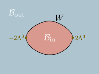
     Figure 1: The space $\mathcal{B}$ in the example of Section 8, divided into two chambers by a wall.

     Since $\mathcal{B}_{\mathrm{in}}$ is simply connected we may trivialize $\Gamma$ over $\mathcal{B}_{\mathrm{in}}$ by primitive cycles $\gamma_{1}$, $\gamma_{2}$ which collapse at the two points of $D$. We choose them so that $\langle\gamma_{1},\gamma_{2}\rangle=1$. The set $\{\gamma_{1},\gamma_{2}\}$ does not extend to a global trivialization of $\Gamma$, since it is not invariant under monodromy. However, the set $\{\gamma_{1},\gamma_{2},\gamma_{1}+\gamma_{2},-\gamma_{1},-\gamma_{2},-\gamma_{1}-\gamma_{2}\}$ is invariant under the monodromy around infinity. Therefore the following definition of $\Omega$ makes global sense:

     $$\text{For }u\in\mathcal{B}_{\mathrm{in}},\,\Omega(\gamma;u) =\begin{cases}1\text{ for }\gamma\in\{\gamma_{1},-\gamma_{1},\gamma_{2},-\gamma_{2}\},\\ 0\text{ otherwise.}\end{cases}$$ (8.4)

     $$\text{For }u\in\mathcal{B}_{\mathrm{out}},\,\Omega(\gamma;u) =\begin{cases}1\text{ for }\gamma\in\{\gamma_{1},-\gamma_{1},\gamma_{2},-\gamma_{2},\gamma_{1}+\gamma_{2},-\gamma_{1}-\gamma_{2}\},\\ 0\text{ otherwise.}\end{cases}$$ (8.5)

   All of our conditions on the data are more or less trivial to check. The most interesting one is the wall-crossing formula (Condition 7). Here the question is: choosing $u_{{\mathrm{in}},{\mathrm{out}}}$ to be two nearby points on opposite sides of $W$, and choosing $V$ to be a narrow sector which contains the rays $\ell_{\gamma_{1}}(u)$ and $\ell_{\gamma_{2}}(u)$ both for $u=u_{\mathrm{in}}$ and for $u=u_{\mathrm{out}}$, do we have

   $$A_{V}(u_{\mathrm{in}})=\mathcal{K}_{\gamma_{1}}\mathcal{K}_{\gamma_{2}}\stackrel{{\scriptstyle?}}{{=}}\mathcal{K}_{\gamma_{2}}\mathcal{K}_{\gamma_{1}+\gamma_{2}}\mathcal{K}_{\gamma_{1}}=A_{V}(u_{\mathrm{out}}).$$ (8.6)

   This identity is indeed true: it is the “pentagon identity” given in [2]. This identity can easily be checked by hand. We remark in passing that (as also noted in [2]) this identity is also closely related to the five-term identity of the dilogarithm function and its quantum counterpart (see e.g. [16, 17].)

   This example has the virtue that for every $u$ only finitely many $\Omega(\gamma;u)$ are nonvanishing. This may lead to some technical simplifications (although we emphasize that there should be no essential difference between this case and the case where there are infinitely many nonvanishing $\Omega(\gamma;u)$, so long as the $\Omega(\gamma;u)$ grow slowly enough with $\gamma$).

   As we commented in the previous section, we expect that the metric $g$ on $\mathcal{M}^{\prime}$ in fact extends to a complete metric on a space $\mathcal{M}$, obtained from $\mathcal{M}^{\prime}$ by adding nodal torus fibers over the two points of $D$, and that the metric around either of these nodal fibers looks like the Ooguri-Vafa metric.

   We believe that this complete metric actually has another name: it is the metric on a certain moduli space of rank-2 Higgs bundles on $\mathbb{C}\mathbb{P}^{1}$ with an irregular singularity at $\infty$. This point of view is discussed at some length in [7]. Also, for any $\zeta\in\mathbb{C}^{\times}$, the complex manifold $(\mathcal{M},J(\zeta))$ is isomorphic to a partial compactification $\mathcal{M}_{0,5}^{\mathrm{cyc}}$ of $\mathcal{M}_{0,5}$, consisting of 5-tuples of points $(z_{1},\dots,z_{5})$ on $\mathbb{C}\mathbb{P}^{1}$ where $z_{i}\neq z_{i+1}$ (with $i$ taken mod $5$). Our description of this space is then closely related to the discussion in [18].

   9 Hitchin systems

   Finally I briefly describe a more geometric family of examples, considered in [7].

   Fix a compact complex smooth curve $\bar{C}$. Fix $n>0$ marked points $z_{i}\in\bar{C}$, and let $C=\bar{C}\setminus\{z_{1},\dots,z_{n}\}$. Also fix parameters $m_{i}\in\mathbb{C}$ and $m_{i}^{(3)}\in\mathbb{R}/2\pi\mathbb{Z}$ associated to the marked points. Assume the $m_{i}$ and $m_{i}^{(3)}$ generic (in particular, the $m_{i}$ should be linearly independent over $\mathbb{Q}$.)

   • $\mathcal{B}$ is the space of meromorphic quadratic differentials $\phi_{2}$ on $\bar{C}$ with double poles at each $z_{i}$, of residue $m_{i}^{2}$. (So $\mathcal{B}$ is a complex affine space.) To stay consistent with our previous notation we will use either $u$ or $\phi_{2}$ to denote a point of $\mathcal{B}$.

   • $D\subset\mathcal{B}$ is the locus of $\phi_{2}$ which have at least one non-simple zero. So $\mathcal{B}^{\prime}$ is the locus of $\phi_{2}$ having only simple zeroes.

   • Let $T^{*}C$ be the holomorphic cotangent bundle to $C$. For any fixed $u\in\mathcal{B}$, consider the noncompact complex curve

     $$\Sigma_{u}=\{(z\in C,\lambda\in T^{*}_{z}C):\lambda^{2}=\phi_{2}(z)\}\subset T^{*}C.$$ (9.1)

     For $u\in\mathcal{B}^{\prime}$, $\Sigma_{u}$ is smooth. The obvious projection $\pi:\Sigma_{u}\to C$ is a double covering, branched over the zeroes of $\phi_{2}$. $\Sigma_{u}$ has a natural compactification $\bar{\Sigma}_{u}$ with a projection $\bar{\pi}:\bar{\Sigma}_{u}\to\bar{C}$.

     $\Sigma_{u}$ is equipped with the involution $\lambda\mapsto-\lambda$. Define $\Gamma_{u}$ to be the subgroup of $H_{1}(\Sigma_{u},\mathbb{Z})$ odd under this involution. $\Gamma_{u}$ is the fiber of a local system $\Gamma$ over $\mathcal{B}^{\prime}$. It is equipped with the intersection pairing $\langle,\rangle$. $\Gamma_{\mathrm{f}}\subset\Gamma$ is the radical of the pairing $\langle,\rangle$, which has rank $n$. This radical does not undergo any monodromy as we vary $u$, so we can think of $\Gamma_{\mathrm{f}}$ as a single fixed lattice rather than a local system. Finally, $\Gamma_{\mathrm{g}}=\Gamma/\Gamma_{\mathrm{f}}$.

   • By slight abuse of notation let $\lambda$ denote the Liouville (tautological) 1-form on $T^{*}C$.

     Then for $\gamma\in\Gamma_{u}$, define

     $$Z(\gamma)=\frac{1}{\pi}\oint_{\gamma}\lambda.$$ (9.2)

   • The 1-form $\lambda$ restricted to $\Sigma_{u}$ extends meromorphically to $\bar{\Sigma}_{u}$, with simple poles at the two preimages of $z_{i}$; let $z_{i}^{\pm}\in\bar{\Sigma}_{u}$ denote the preimage at which $\lambda$ has residue $\pm m_{i}$. The lattice $\Gamma_{\mathrm{f}}$ has one generator $\gamma_{i,{\mathrm{f}}}$ for each puncture $z_{i}$, given by the sum of a counterclockwise loop around $z^{+}_{i}$ and a clockwise loop around $z^{-}_{i}$. We define $\theta_{\mathrm{f}}$ by

     $$\theta_{\mathrm{f}}(\gamma_{i,{\mathrm{f}}})=m_{i}^{(3)}.$$ (9.3)

   • The invariants $\Omega(\gamma;u)$ are defined in terms of the quadratic differential $\phi_{2}$, as follows.

     For any $\vartheta\in\mathbb{R}/2\pi\mathbb{Z}$, define a $\vartheta$-trajectory of $\phi_{2}$ to be a real curve $c\subset C$ such that, for any real tangent vector $v$ to $c$, $\phi_{2}(v\otimes v)\in e^{2{\mathrm{i}}\vartheta}\mathbb{R}_{+}$; call a $\vartheta$-trajectory maximal if it is not properly contained in any other $\vartheta$-trajectory. The maximal $\vartheta$-trajectories make up a singular foliation of $C$, with three-pronged singularities at the zeroes of $\phi_{2}$.

     Define the mass of a maximal $\vartheta$-trajectory $c$ to be $\int_{c}\lvert\sqrt{\phi_{2}}\rvert$. A generic maximal $\vartheta$-trajectory has infinite mass; we are interested in the exceptional trajectories which have finite mass. Let a finite $\vartheta$-trajectory be a maximal $\vartheta$-trajectory with finite mass, and a finite trajectory be a pair $(c,\vartheta)$ where $c$ is a finite $\vartheta$-trajectory. Finite trajectories come in two types:

     • Saddle connections: these are finite trajectories $c$ which “run from one zero of $\phi_{2}$ to another,” i.e., their boundary $\bar{c}\setminus c$ consists of two points (which are then necessarily zeroes of $\phi_{2}$).

     • Closed loops: these are finite trajectories $c$ with the topology of $S^{1}$. When such a trajectory occurs it sits in a 1-parameter family of such trajectories, sweeping out an open annulus on $C$.

     Given a finite trajectory $(c,\vartheta)$, define its lift $\ell(c,\vartheta)$ to be the closure of $\pi^{-1}(c)$ on $\Sigma$. $\ell(c,\vartheta)$ has no boundary; it is a single loop if $(c,\vartheta)$ is a saddle connection (it is enlightening to draw a picture to see why), and the disjoint union of two loops if $(c,\vartheta)$ is a closed loop. The 1-form $e^{-i\vartheta}\lambda$ is real and nonvanishing on $\ell(c,\vartheta)$; hence it induces an orientation on $\ell(c,\vartheta)$. Note that if $(c,\vartheta)$ is a finite trajectory then $(c,\vartheta+\pi)$ is as well, and $\ell(c,\vartheta)$ differs from $\ell(c,\vartheta+\pi)$ only by orientation reversal. By construction, $\ell(c,\vartheta)$ is invariant under the combination of the deck transformation $\lambda\mapsto-\lambda$ and orientation reversal.

     For any $\gamma\in\Gamma_{u}$, let $SC(\gamma;u)$ be the set of all saddle connections $(c,\vartheta)$ with $[\ell(c,\vartheta)]=\gamma$, and let $CL(\gamma;u)$ be the set of all isotopy classes of closed loops $(c,\vartheta)$ with $[\ell(c,\vartheta)]=\gamma$. Now finally we can define

     $$\Omega(\gamma;u)=\#SC(\gamma;u)\,\,-2\#CL(\gamma;u).$$ (9.4)

     (The strange-looking coefficients $+1$ and $-2$ here are really necessary — otherwise the wall-crossing formula (Condition 7) would not be satisfied!)

   These data satisfy all of our Conditions 1-7. The most difficult to see are the last two. Condition 6 follows from known results on quadratic differentials [19, 20] which say $\Omega(\gamma;u)$ grows at most quadratically as a function of the coefficients of $\gamma$. The wall-crossing formula (Condition 7) follows from a sort of inversion of the logic we have followed up to this point: namely, below we will give a direct description of the complex spaces $(\mathcal{M},J(\zeta))$ and the functions $\mathcal{X}_{\gamma}(x,\zeta)$ thereon which solve the Riemann-Hilbert problem and are continuous except at the BPS rays. The existence of such functions $\mathcal{X}_{\gamma}(x,\zeta)$ then implies the wall-crossing formula (following the discussion of Section 4.4).

   In [7] we argued that the hyperkähler space $\mathcal{M}$ in this example is a space of solutions of Hitchin equations on $\bar{C}$, with gauge group $PSU(2)$, and with ramification at the marked points $z_{i}$ (with semisimple residues). This is a much-studied space, considered in particular in [21, 22, 23, 24]. In particular, it is known that the complex spaces $(\mathcal{M},J(\zeta))$ are moduli spaces of $PSL(2,\mathbb{C})$ connections on $C$, with fixed eigenvalues of monodromy around $z_{i}$, given by $\mu_{\pm}=\exp(\pm 2\pi{\mathrm{i}}(\zeta^{-1}m_{i}-m_{i}^{(3)}-\zeta\bar{m}_{i}))$.

   The $\mathcal{X}_{\gamma}(x,\zeta)$ in this example are essentially functions considered earlier by Fock-Goncharov in [25], themselves complexifications of the “shear coordinates” familiar in Teichmüller theory. The main issue in identifying the Fock-Goncharov coordinates with our $\mathcal{X}_{\gamma}(x,\zeta)$ is to prove that the Fock-Goncharov coordinates have the correct asymptotic behavior as $\zeta\to 0,\infty$. This is accomplished by applying the WKB approximation to a family of flat connections on $C$ of the form $\nabla(\zeta)=\varphi/\zeta+D+\bar{\varphi}\zeta$.

   There is a generalization of this story to encompass quadratic differentials with poles of order greater than $2$, also considered in [7]. This generalization in particular includes the “pentagon” example of Section 8; it corresponds to considering quadratic differentials $\varphi_{2}=(z^{3}-3\Lambda^{2}z+u)\mathrm{d}z^{2}$ on $\mathbb{C}\mathbb{P}^{1}$, with order-$7$ poles at $z=\infty$.

   Finally, we have extended many aspects of this story to the case of Hitchin equations with higher rank gauge group $PSU(K)$ [26]. In this case the coordinate functions $\mathcal{X}_{\gamma}$ involve more general coordinate systems than those which were described explicitly by Fock-Goncharov in [25]; conjecturally the $\mathcal{X}_{\gamma}$ exhaust the set of cluster coordinate systems.

   10 DT invariants

   Finally let us briefly consider another viewpoint on this story, which is really where it began. The physical perspective on our construction makes clear that it should be closely related to the theory of generalized Donaldson-Thomas invariants (henceforth just “DT invariants.”) In this section I briefly sketch that relation and a few examples.

   10.1 The dictionary

   In the theory of DT invariants, one begins with a triangulated category $\mathcal{D}$ and constructs the space $\operatorname{Stab}(\mathcal{D})$ of Bridgeland stability conditions on $\mathcal{D}$ [27]. Under some further conditions on $\mathcal{D}$, one then expects to be able to construct DT invariants depending on a point of $\operatorname{Stab}(\mathcal{D})$ [3, 2], whose dependence on the point of $\operatorname{Stab}(\mathcal{D})$ is governed by the wall-crossing formula. In what follows I assume some familiarity with this story and formulate the expected dictionary between the hyperkähler data in our construction and the theory of DT invariants. Many aspects of this dictionary are also described in Section 2.7 of [2].

   We need a few technical preliminaries to “harmonize” the two sides first:

   • On the hyperkähler data side: suppose given an example of our Data 1-6 obeying our Conditions 1-7. Fix a basepoint $u_{0}\in\mathcal{B}^{\prime}$. Let $\tilde{}\mathcal{B}^{\prime}$ denote the universal cover of $\mathcal{B}^{\prime}$. Over this cover we may globally trivialize the local system $\Gamma$, thus identifying all of its fibers with $\Gamma_{u_{0}}$. The fiberwise homomorphism $Z:\Gamma\to\mathbb{C}$ can thus be thought of as a family of homomorphisms from the fixed lattice $\Gamma_{u_{0}}$ to $\mathbb{C}$, depending on a point $\tilde{u}\in\tilde{\mathcal{B}^{\prime}}$,

     $$Z(\tilde{u}):\Gamma_{u_{0}}\to\mathbb{C}.$$ (10.1)

   • On the DT theory side: suppose given an appropriate category $\mathcal{D}$. $\operatorname{Stab}(\mathcal{D})$ is a complex Poisson manifold, carrying a natural “forgetful” map to $\operatorname{Hom}(K(\mathcal{D}),\mathbb{C})$ which is a local Poisson isomorphism [27]. We will consider a single connected component $\operatorname{Stab}^{0}(\mathcal{D})\subset\operatorname{Stab}(\mathcal{D})$.

   We then have the following expected dictionary:

   DT theory	hyperkähler data
   $K(\mathcal{D})$	$\Gamma_{u_{0}}$
   Euler pairing	$\langle\cdot,\cdot\rangle$
   stability functions $Z:K(\mathcal{D})\to\mathbb{C}$	$Z(\tilde{u}):\Gamma_{u_{0}}\to\mathbb{C}$
   DT invariants of $\mathcal{D}$	$c(\gamma)\in\mathbb{Q}$ from (4.9)
   a quotient of a Lagrangian $L\subset\operatorname{Stab}^{0}(\mathcal{D})$	$\mathcal{B}^{\prime}$
   ???	$\mathcal{B}$
   ???	$\theta_{\mathrm{f}}$

   
   

   This dictionary has one especially awkward feature: starting from the category $\mathcal{D}$ it is not at all clear how to choose the complex Lagrangian submanifold $L$. Because of this problem, at the moment we do not really have a recipe which begins with $\mathcal{D}$ alone and constructs a corresponding hyperkähler space. In particular examples which we do understand, $L$ always has some nice geometric meaning (see the next section). It would be very interesting to understand how to get $L$ in a purely categorical way.

   10.2 Examples

   For many examples of our construction of hyperkähler metrics (probably in all the examples that come from an underlying supersymmetric quantum field theory, which includes all of the examples discussed so far in this note), we expect that there is some triangulated category $\mathcal{D}$, fitting into the above dictionary. Let us now describe a few examples:

   • Let $\mathcal{D}$ be the category of finite-dimensional modules over the Ginzburg dg algebra of the $A_{2}$ quiver. In recent work of Sutherland [28], one connected component $\operatorname{Stab}^{0}(\mathcal{D})\subset\operatorname{Stab}(\mathcal{D})$ is identified with the universal cover of the total space of a particular $\mathbb{C}^{\times}$ bundle over the moduli space $\mathcal{M}_{1,1}$ of elliptic curves. This result fits well into the above dictionary: indeed we claim that the hyperkähler data corresponding to the category $\mathcal{D}$ is that of the “pentagon” example of Section 8 above. The elliptic curves appearing in Sutherland’s picture are the curves $\Sigma_{u}$ of Section 8.

   • Recent work of Bridgeland and Smith [29] is also relevant to this dictionary.

     Begin with a real compact 2-manifold $C$, with $n>1$ marked points. From the combinatorics of ideal triangulations of the curve $C$, one can build an associated quiver $Q(C)$, using a superpotential function first written down by Labardini-Fragoso [30]. Let $\mathcal{D}(C)$ be the derived category of finite-dimensional modules over the Ginzburg dg algebra of $Q(C)$. Bridgeland and Smith show (roughly — for the precise statement see [29]) that there is a component $\operatorname{Stab}^{0}(\mathcal{D}(C))\subset\operatorname{Stab}(\mathcal{D}(C))$, such that a point of $\operatorname{Stab}^{0}(\mathcal{D}(C))$ corresponds to a choice of complex structure on $C$ and a meromorphic quadratic differential thereon, with double poles at the marked points. Among other things, this provides a family of nontrivial examples of categories $\mathcal{D}$ where one has a geometric interpretation for at least a component of $\operatorname{Stab}(\mathcal{D})$.

     This result fits in well with the dictionary proposed above: it is consistent with the idea that the categories $\mathcal{D}(C)$ correspond to the hyperkähler data described in Section 9. Moreover, revisiting Section 9 we see that the mysterious Lagrangian subspace $L\subset\operatorname{Stab}(\mathcal{D}(C))$ appearing in the dictionary has a nice meaning here: it corresponds to fixing a particular complex structure on $C$ and a choice of residues at the marked points on $C$.

     Bridgeland and Smith also consider a generalization corresponding to allowing meromorphic quadratic differentials with higher-order poles. This generalization in particular gives another proof of Sutherland’s results from [28] (by considering quadratic differentials on $\mathbb{C}\mathbb{P}^{1}$ with a single pole of order $7$).

   • More ambitiously, at least on physical grounds we expect that given a complete non-compact Calabi-Yau threefold $X$, both sides of this dictionary should exist. Roughly speaking, $\mathcal{D}=\mathcal{D}(X)$ should be an appropriate version of the Fukaya category of $X$; $\mathcal{B}$ should be the moduli space of complex structures in $X$; $\Gamma$ should be $H_{3}(X,\mathbb{Z})$; $Z$ should be the period map; $c(\gamma)$ should be DT invariants counting special Lagrangian 3-cycles in $X$. The Lagrangian submanifold $L$ is the period domain of $X$; the fact that it is Lagrangian is essentially Griffiths transversality. Finally, the hyperkähler space $\mathcal{M}$ built by our construction is some version of the family of intermediate Jacobians of $X$ (I say “some version” because we are dealing with non-compact $X$).

     The examples studied by Bridgeland and Smith, i.e. the examples of Section 9 above, also fall into this class. The Calabi-Yau threefold $X(C)$ in this case is a conic bundle over the curve $C$, appropriately modified at the marked points; the Fukaya category $\mathcal{D}(X(C))$ is equivalent to the category $\mathcal{D}(C)$ mentioned above. This equivalence will also be explained in upcoming work of Bridgeland and Smith.

     (Incidentally, following through our various claims about the hyperkähler space $\mathcal{M}$ in these examples, we see that on the one hand $\mathcal{M}$ should be a version of the family of intermediate Jacobians of $X(C)$, while on the other hand $\mathcal{M}$ should be the $PSU(2)$ Hitchin system on $C$, with ramification at the marked points. So our claims would imply that these two integrable systems the same. This equivalence is not really novel: a version of it without the marked points was described in [32], a fact which gives us some additional confidence in our whole picture.)

     For general $X$, it is not clear a priori that the DT invariants will grow slowly enough to satisfy our Condition 6. Nevertheless, on physical grounds we would expect the hyperkähler manifold $\mathcal{M}$ to exist for general $X$. Thus we expect that either the DT invariants do in fact grow slowly enough for us to prove that the Riemann-Hilbert problem has a solution, or they grow more quickly but have some hidden extra structure that allows the Riemann-Hilbert problem to have a solution anyway.

   • Finally let me describe a non-example. It is natural to ask: what if we let $\mathcal{D}$ be the Fukaya category of a compact Calabi-Yau threefold $X$ — will there be corresponding hyperkähler data then? It seems that the answer is “yes” — we can define the data by the same recipe as we use for non-compact $X$ — but these data would not satisfy precisely our Conditions 1-7. In particular, Condition 4 (positive definiteness) will certainly be violated. However, this violation is of a rather controlled sort; there is just one negative direction. So, were this the only difficulty, the expected consequence would be that the space $\mathcal{M}$ we obtain is not hyperkähler but pseudo-hyperkähler, with one negative direction. ($\mathcal{M}$ in this case is the family of intermediate Jacobians of $X$, fibered over the moduli space of polarized complex structures on $X$. These intermediate Jacobians are quotients of $H^{3,0}\oplus H^{2,1}(X)$, and the negative direction is coming from $H^{3,0}(X)$; it is related to the fact that when equipped with its “Griffiths” complex structure, the intermediate Jacobian is not principally polarized.) However, there is also a second, more serious difficulty: the invariants $\Omega(\gamma)$ counting special Lagrangian 3-cycles in $X$ are expected to grow very quickly as functions of $\gamma$ (roughly $\Omega(\gamma)\sim\exp c\lVert\gamma\rVert^{2}$), badly violating our Condition 6. As a result it is far from clear whether our construction of hyperkähler metrics should be directly applicable to this situation.

     This difficulty is in some sense anticipated in the physics literature. Indeed, physics does not predict directly that there is an hyperkähler manifold associated to a compact Calabi-Yau threefold $X$. Rather it predicts the existence of a quaternionic-Kähler manifold. As in the hyperkähler case, it should be possible to construct the desired quaternionic-Kähler structure by beginning with a simple “semi-flat” metric $g^{\mathrm{sf}}$ and modifying it by quantum corrections. The semi-flat metric in this case was first described by Ferrara and Sabharwal in [33], and was recently discussed by Hitchin in [34]. The description of the quantum corrections has been studied intensely in physics, with various interesting partial results. In particular, some of the quantum corrections are expected to be precise analogues of the ones we have described in the hyperkähler case, indeed related by a “quaternionic-Kähler/hyperkähler correspondence” [35, 36]. However, one also expects new quantum corrections in the quaternionic-Kähler case which do not have an hyperkähler analogue. As far as I know, there are no examples yet of $X$ where all quantum corrections have been fully described.

References

- [1] D. Gaiotto, G. W. Moore, and A. Neitzke, “Four-dimensional wall-crossing via three-dimensional field theory,” 0807.4723.
- [2] M. Kontsevich and Y. Soibelman, “Stability structures, motivic Donaldson-Thomas invariants and cluster transformations,” 0811.2435.
- [3] D. Joyce and Y. Song, “A theory of generalized Donaldson-Thomas invariants,” 0810.5645.
- [4] M. Gross and P. M. H. Wilson, “Large complex structure limits of surfaces,” J. Differential Geom. 55 (2000), no. 3, 475–546.
- [5] M. Kontsevich and Y. Soibelman, “Homological mirror symmetry and torus fibrations,” in Symplectic geometry and mirror symmetry (Seoul, 2000), pp. 203–263. World Sci. Publ., River Edge, NJ, 2001.
- [6] A. Strominger, S.-T. Yau, and E. Zaslow, “Mirror symmetry is T-duality,” Nucl. Phys. B479 (1996) 243–259, hep-th/9606040.
- [7] D. Gaiotto, G. W. Moore, and A. Neitzke, “Wall-crossing, Hitchin Systems, and the WKB Approximation,” 0907.3987.
- [8] S. Cecotti, S. Ferrara, and L. Girardello, “Geometry of type II superstrings and the moduli of superconformal field theories,” Int. J. Mod. Phys. A4 (1989) 2475.
- [9] D. S. Freed, “Special Kähler manifolds,” Commun. Math. Phys. 203 (1999) 31–52, hep-th/9712042.
- [10] B. R. Greene, A. D. Shapere, C. Vafa, and S.-T. Yau, “Stringy cosmic strings and noncompact Calabi-Yau manifolds,” Nucl. Phys. B337 (1990) 1.
- [11] B. Dubrovin, “Geometry and integrability of topological-antitopological fusion,” Commun. Math. Phys. 152 (1993), no. 3, 539–564, hep-th/9206037.
- [12] S. Cecotti and C. Vafa, “On classification of supersymmetric theories,” Commun. Math. Phys. 158 (1993) 569–644, hep-th/9211097.
- [13] N. J. Hitchin, A. Karlhede, U. Lindstrom, and M. Roček, “Hyperkähler metrics and supersymmetry,” Commun. Math. Phys. 108 (1987) 535.
- [14] N. Hitchin, “Hyper-Kähler manifolds,” Astérisque (1992), no. 206, Exp. No. 748, 3, 137–166. Séminaire Bourbaki, Vol. 1991/92.
- [15] H. Ooguri and C. Vafa, “Summing up D-instantons,” Phys. Rev. Lett. 77 (1996) 3296–3298, hep-th/9608079.
- [16] L. D. Faddeev and R. M. Kashaev, “Quantum dilogarithm,” Mod. Phys. Lett. A9 (1994) 427–434, hep-th/9310070.
- [17] D. Zagier, “The dilogarithm function,” in Frontiers in number theory, physics, and geometry. II, pp. 3–65. Springer, Berlin, 2007.
- [18] A. B. Goncharov, “Pentagon relation for the quantum dilogarithm and quantized ,” 0706.4054.
- [19] H. Masur, “The growth rate of trajectories of a quadratic differential,” Ergodic Theory Dynam. Systems 10 (1990), no. 1, 151–176.
- [20] A. Eskin and H. Masur, “Asymptotic formulas on flat surfaces,” Ergodic Theory Dynam. Systems 21 (2001), no. 2, 443–478.
- [21] N. J. Hitchin, “The self-duality equations on a Riemann surface,” Proc. London Math. Soc. (3) 55 (1987), no. 1, 59–126.
- [22] K. Corlette, “Flat -bundles with canonical metrics,” J. Differential Geom. 28 (1988), no. 3, 361–382.
- [23] S. K. Donaldson, “Twisted harmonic maps and the self-duality equations,” Proc. London Math. Soc. (3) 55 (1987), no. 1, 127–131.
- [24] C. Simpson, “Harmonic bundles on noncompact curves,” J. Amer. Math. Soc. 3 (1990) 713–770.
- [25] V. Fock and A. Goncharov, “Moduli spaces of local systems and higher Teichmüller theory,” Publ. Math. Inst. Hautes Études Sci. (2006), no. 103, 1–211, math/0311149.
- [26] D. Gaiotto, G. W. Moore, and A. Neitzke, “Spectral networks,” 1204.4824.
- [27] T. Bridgeland, “Stability conditions on triangulated categories,” Annals Math. 166-2 (2002) 317–345, math.AG/0212237.
- [28] T. Sutherland, “The modular curve as the space of stability conditions of a CY3 algebra,” 1111.4184.
- [29] T. Bridgeland and I. Smith, “Quadratic differentials as stability conditions,” 1302.7030.
- [30] D. Labardini-Fragoso, “Quivers with potentials associated to triangulated surfaces,” 0803.1328.
- [31] M. Alim, S. Cecotti, C. Cordova, S. Espahbodi, A. Rastogi, and C. Vafa, “BPS Quivers and Spectra of Complete Quantum Field Theories,” 1109.4941.
- [32] D.-E. Diaconescu, R. Donagi, and T. Pantev, “Intermediate jacobians and ade hitchin systems,” hep-th/0607159.
- [33] S. Ferrara and S. Sabharwal, “Quaternionic manifolds for type II superstring vacua of Calabi-Yau spaces,” Nucl. Phys. B332 (1990) 317.
- [34] N. Hitchin, “Quaternionic Kähler moduli spaces,” in Riemannian topology and geometric structures on manifolds, vol. 271 of Progr. Math., pp. 49–61. Birkhäuser Boston, Boston, MA, 2009.
- [35] S. Alexandrov, D. Persson, and B. Pioline, “Wall-crossing, Rogers dilogarithm, and the QK/HK correspondence,” 1110.0466.
- [36] A. Haydys, “HyperKähler and quaternionic Kähler manifolds with -symmetries,” J. Geom. Phys. 58 (2008), no. 3, 293–306, 0706.4473.
-
Condition 6: