Nitsche’s method for two and three dimensional NURBS patch coupling

Abstract

A Nitche’s method is presented to couple non-conforming two and three dimensional NURBS (Non Uniform Rational B-splines) patches in the context of isogeometric analysis (IGA). We present results for elastic stress analyses under the static condition of two and three dimensional NURBS geometries. The contribution fills the gap in the literature and enlarges the applicability of NURBS-based isogeometric analysis.

1 Introduction

The predominant technology that is used by CAD to represent complex geometries is the Non-Uniform Rational B-spline (NURBS). This allows certain geometries to be represented exactly that are only approximated by polynomial functions, including conic and circular sections. There is a vast array of literature focused on NURBS (e.g. [1], [2]) and as a result of several decades of research, many efficient computer algorithms exist for their fast evaluation and refinement. The key concept outlined by Hughes et al. [3] was to employ NURBS not only as a geometry discretisation technology, but also as a discretisation tool for analysis, attributing such methods to the field of ‘Isogeometric Analysis’ (IGA). Since this seminal paper, a monograph dedicated entirely to IGA has been published [4] and applications can now be found in several fields including structural mechanics, solid mechanics, fluid mechanics and contact mechanics. It should be emphasized that the idea of using CAD technologies in finite elements dates back at least to [5, 6] where B-splines were used as shape functions in FEM. In addition, similar methods which adopt subdivision surfaces have been used to model shells [7].

Structural mechanics is a field where IGA has demonstrated compelling benefits over conventional approaches [8, 9, 10, 11, 12, 13, 14]. The smoothness of the NURBS basis functions allows for a straightforward construction of plate/shell elements. Particularly for thin shells, rotation-free formulations can be easily constructed [9, 15]. Furthermore, isogeometric plate/shell elements exhibit much less pronounced shear-locking compared to standard FE plate/shell elements.

In contact formulations using conventional geometry discretisations, the presence of faceted surfaces can lead to jumps and oscillations in traction responses unless very fine meshes are used. The benefits of using NURBS over such an approach are evident, since smooth contact surface are obtained, leading to more physically accurate contact stresses. Recent work in this area includes [16, 17, 18, 19, 20].

IGA has also shown advantages over traditional approaches in the context of optimisation problems [21, 22, 23, 24] where the tight coupling with CAD models offers an extremely attractive approach for industrial applications. Another attractive class of methods include those that require only a boundary discretisation, creating a truly direct coupling with CAD. Isogeometric boundary element methods for elastostatic analysis were presented in [25, 26], demonstrating that mesh generation can be completely circumvented by using CAD discretisations for analysis.

The smoothness of NURBS basis functions is attractive for analysis of fluids [27, 28, 29] and for fluid-structure interaction problems [30, 31]. In addition, due to the ease of constructing high order continuous basis functions, IGA has been used with great success in solving PDEs that incorporate fourth order (or higher) derivatives of the field variable such as the Hill-Cahnard equation [32], explicit gradient damage models [33] and gradient elasticity [34]. The high order NURBS basis has also found potential applications in the Kohn-Sham equation for electronic structure modeling of semiconducting materials [35].

NURBS provide advantageous properties for structural vibration problems [36, 37, 38, 39] where $k$-refinement (unique to IGA) has been shown to provide more robust and accurate frequency spectra than typical higher-order FE $p$-methods. Particularly, the optical branches of frequency spectra, which have been identified as contributors to Gibbs phenomena in wave propagation problems (and the cause of rapid degradation of higher modes in the $p$-version of FEM), are eliminated. However when lumped mass matrices were used, the accuracy is limited to second order for any basis order. High order isogeometric lumped mass matrices are not yet available. The mathematical properties of IGA were studied in detail by Evans et al.[40].

IGA has been applied to cohesive fracture [41], outlining a framework for modeling debonding along material interfaces using NURBS and propagating cohesive cracks using T-splines. The method relies upon the ability to specify the continuity of NURBS and T-splines through a process known as knot insertion. As a variation of the eXtended Finite Element Method (XFEM) [42], IGA was applied to Linear Elastic Fracture Mechanics (LEFM) using the partition of unity method (PUM) to capture two dimensional strong discontinuities and crack tip singularities efficiently [43, 44]. The method is usually referred to as XIGA (eXtended IGA). In [45] an explicit isogeometric enrichment technique was proposed for modeling material interfaces and cracks exactly. Note that this method is contrary to PUM-based enrichment methods which define cracks implicitly. A phase field model for dynamic fracture was presented in [46] using adaptive T-spline refinement to provide an effective method for simulating fracture in three dimensions. In [47] high order B-splines were adopted to efficiently model delamination of composite specimens and in [48], an isogeometric framework for two and three dimensional delamination analysis of composite laminates was presented where the authors showed that using IGA can significantly reduce the usually time consuming pre-processing step in generating FE meshes (solid elements and cohesive interface elements) for delamination computations. A continuum description of fracture using explicit gradient damage models was also studied using NURBS [33].

In computer aided geometric design, objects of complex topologies are usually represented as multiple-patch NURBS. We refer to Fig. 1 for such a multi-patch NURBS solid. Since it is virtually impossible to have a conforming parametrisation at the patch interface, an important research topic within the IGA context is the implementation of multi-patch methods with high inter-patch continuity properties. In this paper, a Nitsche’s method is presented to couple non-conforming two and three dimensional NURBS patches in a weak sense. An exact multipoint constraint method was reported in [4] to glue multiple NURBS patches with the restriction that, in the coarsest mesh, they have the same parametrisation. Another solution to multi-patch IGA which has gathered momentum from both the computational geometry and analysis communities is the use of T-splines [49]. T-splines correct the deficiencies of NURBS by creating a single patch, watertight geometry which can be locally refined and coarsened. Utilisation of T-splines in an IGA framework has been illustrated in [50, 51, 52]. However T-splines are not yet a standard in CAD and therefore our contribution will certainly enlarge the application areas of NURBS based IGA. Moreover, the formulation presented in this contribution lays the foundation for the solid-structure coupling method to be presented in a forthcoming paper [53].

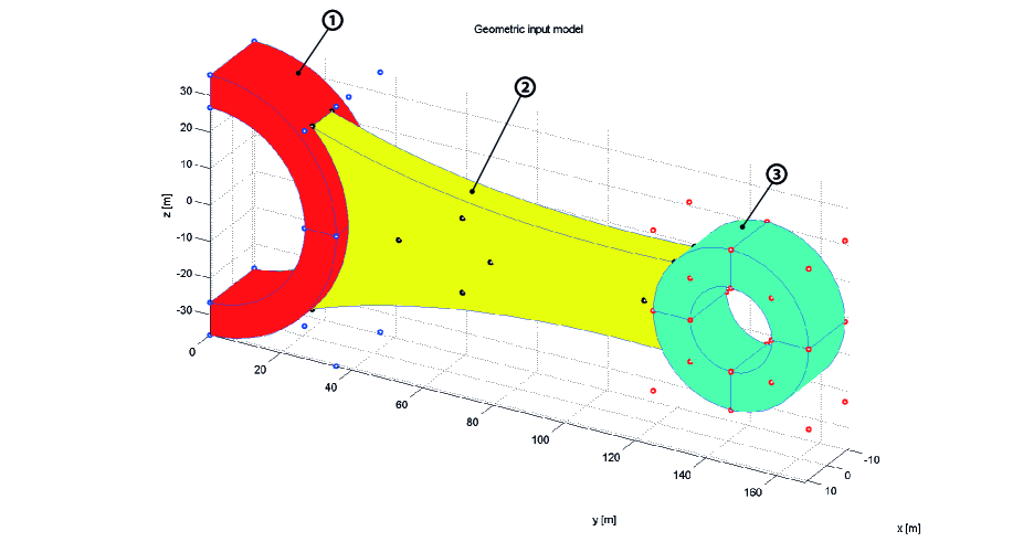
Figure 1: A multi-patch NURBS solid.

Nitsche’s method [54] was originally proposed to weakly enforce Dirichlet boundary conditions as an alternative to equivalent pointwise constraints. The idea behind a Nitsche based approach is to replace the Lagrange multipliers arising in a dual formulation through their physical representation, namely the normal flux at the interface. Nitsche also added an extra penalty like term to restore the coercivity of the bilinear form. The method can be seen to lie in between the Lagrange multiplier method and the penalty method. The method has seen a resurgence in recent years and was applied for interface problems [55, 56], for connecting overlapping meshes [57, 58, 59, 60], for imposing Dirichlet boundary conditions in meshfree methods [61], in immersed boundary methods [62, 63, 64], in fluid mechanics [65], in the Finite Cell Method [66] and for contact mechanics [67]. It has also been applied for stabilising constraints in enriched finite elements [68].

The remainder of the paper is organised as follows. The problem description, governing equations and weak formulation are presented in Section 2. Section 3 discusses the discretisation followed by implementation aspects given in Section 4. Several two and three dimensional examples are given in Section 5.

We denote $d_{p}$ and $d_{s}$ as the number of parametric directions and spatial directions respectively. Both tensor and matrix notations are used. In tensor notation, tensors of order one or greater are written in boldface. Lower case bold-face letters are used for first-order tensor whereas upper case bold-face letters indicate high-order tensors. The major exception to this rule are the physical second order stress tensor and the strain tensor which are written in lower case. In matrix notation, the same symbols as for tensors are used to denote the matrices but the connective operator symbols are skipped.

2 Problem description, governing equations and weak form

2.1 Governing equations

We define the domain $\Omega\subset\mathbb{R}^{d_{s}}$ with boundary $\Gamma\equiv\partial\Omega$. For sake of simplicity, we assume there is only one internal boundary denoted by $\Gamma_{*}$ that divides the domain into two non-overlapping domains $\Omega^{m},m=1,2$ such that $\Omega=\Omega^{1}\cup\Omega^{2}$. In the context of multi-patch NURBS IGA, each domain represents a NURBS patch. Excluding $\Gamma_{*}$, the rest of $\Gamma$ can be divided into Dirichlet and Neumann parts on each domain, $\Gamma_{u}^{m}$ and $\Gamma_{t}^{m}$ respectively. A superscript, $m$, is used to denote a quantity that is valid over region $\Omega^{m}$, with $m=1,2$.

With the primary unknown displacement field $\mathbf{u}^{m}$, the governing equations of linear elastostatic problems are

$$-\nabla\;\boldsymbol{\sigma}^{m} =\mathbf{b}^{m} \quad\text{on}\quad\Omega^{m}$$ (1a)

$$\mathbf{u}^{m} =\bar{\mathbf{u}}^{m} \quad\text{on}\quad\Gamma_{u}^{m}$$ (1b)

$$\boldsymbol{\sigma}^{m}\cdot\mathbf{n}^{m} =\bar{\mathbf{t}}^{m} \quad\text{on}\quad\Gamma_{t}^{m}$$ (1c)

$$\mathbf{u}^{1} =\mathbf{u}^{2} \quad\text{on}\quad\Gamma_{*}$$ (1d)

$$\boldsymbol{\sigma}^{1}\cdot\mathbf{n}^{1} =-\boldsymbol{\sigma}^{2}\cdot\mathbf{n}^{2} \quad\text{on}\quad\Gamma_{*}$$ (1e)

where $\boldsymbol{\sigma}^{m}$ denotes the stress field; the last two equations express the continuity of displacements and tractions across $\Gamma_{*}$. The prescribed displacement and traction are denoted by $\bar{\mathbf{u}}^{m}$ and $\bar{\mathbf{t}}^{m}$, respectively. The outward unit normals to $\Omega^{1}$ and $\Omega^{2}$ are $\mathbf{n}^{1}$ and $\mathbf{n}^{2}$, respectively.

Under the small strain condition, the infinitesimal strain tensor reads $\boldsymbol{\epsilon}^{m}=0.5(\nabla\mathbf{u}^{m}+\nabla^{\mathrm{T}}\mathbf{u}^{m})$. Constitutive equations are given by

$$\boldsymbol{\sigma}^{m}=\mathbf{C}^{m}:\boldsymbol{\epsilon}^{m},\quad m=1,2$$ (2)

where the constitutive tensors are denoted by $\mathbf{C}^{1}$ and $\mathbf{C}^{2}$. For linear isotropic elastic materials, the constitutive tensor is written as

$$C_{ijkl}=\lambda\delta_{ik}\delta_{kl}+\mu(\delta_{ik}\delta_{jl}+\delta_{il}\delta_{jk})$$ (3)

where $\lambda=\frac{E\nu}{(1+\nu)(1-2\nu)}$ and $\mu=\frac{E}{2(1+\nu)}$ are the Lamé constants; $E$ and $\nu$ are the Young’s modulus and Poisson’s ratio, respectively and $\delta_{ij}$ is the Kronecker delta tensor.

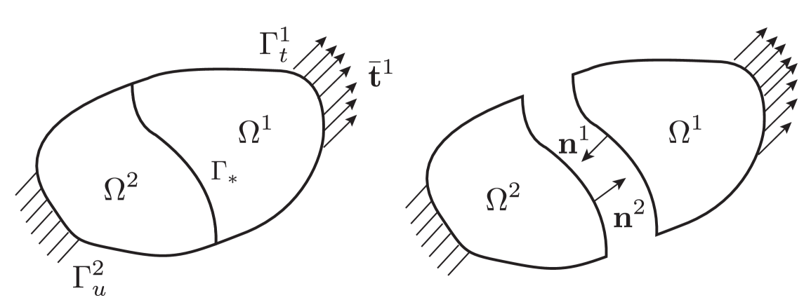
Figure 2: Computational domain with an internal interface.

2.2 Weak form

We start by defining the spaces, $\boldsymbol{S}^{m}$ and $\mathbf{V}^{m}$ over domain $\Omega^{m}$ that will contain the solution and trial functions respectively:

$$\begin{split}\boldsymbol{S}^{m}&=\{\mathbf{u}^{m}(\mathbf{x})|\mathbf{u}^{m}(\mathbf{x})\in\boldsymbol{H}^{1}(\Omega^{m}),\mathbf{u}^{m}=\bar{\mathbf{u}}^{m}\;\;\text{on $\Gamma_{u}^{m}$}\}\\ \boldsymbol{V}^{m}&=\{\mathbf{w}^{m}(\mathbf{x})|\mathbf{w}^{m}(\mathbf{x})\in\boldsymbol{H}^{1}(\Omega^{m}),\mathbf{w}^{m}={\mathbf{0}}\;\;\text{on $\Gamma_{u}^{m}$}\}\end{split}$$ (4)

The standard application of Nitsche’s method for the coupling is: Find $(\mathbf{u}^{1},\mathbf{u}^{2})\in\boldsymbol{S}^{1}\times\boldsymbol{S}^{2}$ such that

$$\sum_{m=1}^{2}\int_{\Omega^{m}}\boldsymbol{\epsilon}(\mathbf{w}^{m}):\boldsymbol{\sigma}^{m}\mathrm{d}\Omega-\int_{\Gamma^{*}}\left([\![{\mathbf{w}}]\!]\otimes\mathbf{n}^{1}\right):\{\boldsymbol{\sigma}\}\mathrm{d}\Gamma-\int_{\Gamma^{*}}\left([\![{\mathbf{u}}]\!]\otimes\mathbf{n}^{1}\right):\{\boldsymbol{\sigma}(\mathbf{w})\}\mathrm{d}\Gamma\\ +\int_{\Gamma^{*}}\alpha[\![{\mathbf{w}}]\!]\cdot[\![{\mathbf{u}}]\!]\mathrm{d}\Gamma=\sum_{m=1}^{2}\int_{\Omega^{m}}\mathbf{w}^{m}\cdot\mathbf{b}^{m}\mathrm{d}\Omega+\sum_{m=1}^{2}\int_{\Gamma_{t}^{m}}\mathbf{w}^{m}\cdot\bar{\mathbf{t}}^{m}\mathrm{d}\Gamma$$ (5)

for all $(\mathbf{w}^{1},\mathbf{w}^{2})\in\boldsymbol{V}^{1}\times\boldsymbol{V}^{2}$. Derivation of this weak form is standard and can be found in, for example, [60]. Note that we have assumed that essential boundary conditions are enforced point-wise if possible or by other methods than Nitsche’s method for we want to focus on the patch coupling.

In Equation (5), the jump and average operators, on the interface $\Gamma^{*}$, $[\![{\cdot}]\!]$ and $\{\cdot\}$ are defined as

$$[\![{\mathbf{u}}]\!]=\mathbf{u}^{1}-\mathbf{u}^{2},\quad\{\boldsymbol{\sigma}\}=\frac{1}{2}(\boldsymbol{\sigma}^{1}+\boldsymbol{\sigma}^{2})$$ (6)

For completeness, note that the average operator for the stress field can be written generally as [59]

$$\{\boldsymbol{\sigma}\}=\gamma\boldsymbol{\sigma}^{1}+(1-\gamma)\boldsymbol{\sigma}^{2}$$ (7)

where $0\leq\gamma\leq 1$. The usual average operator is reproduced if $\gamma=0.5$ is used. Equation (7) is often utilized to join a soft model and a stiff one [60]. Taking $\gamma=1$ (or $\gamma=0$) results in the one-sided mortaring method. In this paper, the standard average operator is used unless otherwise stated.

Except the second and third terms in the left hand side, Equation (5) is the same as the penalty method. As in the penalty method, $\alpha$ is a free parameter for Nitsche’s method. However, rather than being a penalty parameter, it should be viewed as a stabilization parameter in the context of this method. It has been shown [69] that a minimum $\alpha$ exists that will guarantee the positive definiteness of the bilinear form associated with Nitsche’s method, thus, the stability of the method.

For discretisation we rewrite Equation (5) in a matrix form as follows: Find $(\mathbf{u}^{1},\mathbf{u}^{2})\in\boldsymbol{S}^{1}\times\boldsymbol{S}^{2}$ such that

$$\sum_{m=1}^{2}\int_{\Omega^{m}}(\boldsymbol{\epsilon}(\mathbf{w}^{m}))^{\mathrm{T}}\boldsymbol{\sigma}^{m}\mathrm{d}\Omega-\int_{\Gamma_{*}}[\![{\mathbf{w}}]\!]^{\mathrm{T}}\mathbf{n}\{\boldsymbol{\sigma}\}\mathrm{d}\Gamma-\int_{\Gamma_{*}}\{\boldsymbol{\sigma}(\mathbf{w})\}^{\mathrm{T}}\mathbf{n}^{\mathrm{T}}[\![{\mathbf{u}}]\!]\mathrm{d}\Gamma\\ +\int_{\Gamma_{*}}\alpha[\![{\mathbf{w}}]\!]^{\mathrm{T}}[\![{\mathbf{u}}]\!]\mathrm{d}\Gamma=\sum_{m=1}^{2}\int_{\Gamma_{t}^{m}}(\mathbf{w}^{m})^{\mathrm{T}}\bar{\mathbf{t}}^{m}\mathrm{d}\Gamma+\sum_{m=1}^{2}\int_{\Omega^{m}}(\mathbf{w}^{m})^{\mathrm{T}}\mathbf{b}^{m}\mathrm{d}\Omega$$ (8)

for all $(\mathbf{w}^{1},\mathbf{w}^{2})\in\boldsymbol{V}^{1}\times\boldsymbol{V}^{2}$. Superscript T denotes the transpose operator. Second order tensors ($\sigma_{ij}$ and $\epsilon_{ij}$) are written using the Voigt notation as column vectors; $\boldsymbol{\sigma}=[\sigma_{xx},\sigma_{yy},\sigma_{zz},\sigma_{xy},\sigma_{yz},\sigma_{xz}]^{\mathrm{T}}$, $\boldsymbol{\epsilon}=[\epsilon_{xx},\epsilon_{yy},\epsilon_{zz},2\epsilon_{xy},2\epsilon_{yz},2\epsilon_{xz}]^{\mathrm{T}}$, and $\mathbf{n}$ (note that we removed the subscript 1 for subsequent derivations) is a matrix that reads

$$\mathbf{n}_{2D}=\begin{bmatrix}n_{x}&0&n_{y}\\ 0&n_{y}&n_{x}\end{bmatrix},\quad\mathbf{n}_{3D}=\begin{bmatrix}n_{x}&0&0&n_{y}&0&n_{z}\\ 0&n_{y}&0&n_{x}&n_{z}&0\\ 0&0&n_{z}&0&n_{y}&n_{x}\end{bmatrix}$$ (9)

for two dimensions and three dimensions, respectively.

3 Discretisation

3.1 NURBS

In this section, NURBS are briefly reviewed. We refer to the standard textbook [1] for details. A knot vector is a sequence in ascending order of parameter values, written $\Xi=\{\xi_{1},\xi_{2},\ldots,\xi_{n+p+1}\}$ where $\xi_{i}$ is the ith knot, $n$ is the number of basis functions and $p$ is the order of the B-spline basis. Open knots in which the first and last knots appear $p+1$ times are standard in the CAD literature and thus used in this manuscript i.e., $\Xi=\{\underbrace{\xi_{1},\ldots,\xi_{1}}_{\text{$p+1$ times}},\xi_{2},\ldots,\underbrace{\xi_{m},\ldots\xi_{m}}_{\text{$p+1$ times}}\}$.

Given a knot vector $\Xi$, the B-spline basis functions are defined recursively starting with the zeroth order basis function ($p=0$) given by

$$N_{i,0}(\xi)=\begin{cases}1&\textrm{if $\xi_{i}\leq\xi<\xi_{i+1}$}\\ 0&\textrm{otherwise}\end{cases}$$ (10)

and for a polynomial order $p\geq 1$

$$N_{i,p}(\xi)=\frac{\xi-\xi_{i}}{\xi_{i+p}-\xi_{i}}N_{i,p-1}(\xi)+\frac{\xi_{i+p+1}-\xi}{\xi_{i+p+1}-\xi_{i+1}}N_{i+1,p-1}(\xi)$$ (11)

This is referred to as the Cox-de Boor recursion formula. Note that when evaluating these functions, ratios of the form $0/0$ are defined as zero.

Some salient properties of B-spline basis functions are (1) they constitute a partition of unity, (2) each basis function is nonnegative over the entire domain, (3) they are linearly independent, (4) the support of a B-spline function of order $p$ is $p+1$ knot spans i.e., $N_{i,p}$ is non-zero over $[\xi_{i},\xi_{i+p+1}]$, (5) basis functions of order $p$ have $p-m_{i}$ continuous derivatives across knot $\xi_{i}$ where $m_{i}$ is the multiplicity of knot $\xi_{i}$ and (6) B-spline basis are generally only approximants (except at the ends of the parametric space interval, $[\xi_{1},\xi_{n+p+1}]$) and not interpolants.

Fig. 3 illustrates a corresponding set of basis functions for an open, non-uniform knot vector. Of particular note is the interpolatory nature of the basis function at each end of the interval created through an open knot vector, and the reduced continuity at $\xi=4$ due to the presence of the location of a repeated knot where $C^{0}$ continuity is attained. Elsewhere, the functions are $C^{1}$ continuous ($C^{p-1}$).

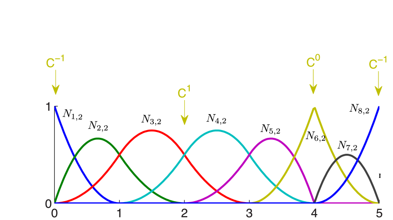
Figure 3: Quadratic B-spline basis functions defined for the open, non-uniform knot vector $\Xi=\{0,0,0,1,2,3,4,4,5,5,5\}$. Note the flexibility in the construction of basis functions with varying degrees of regularity.

NURBS basis functions are defined as

$$R_{i,p}(\xi)=\frac{N_{i,p}(\xi)w_{i}}{W(\xi)}=\frac{N_{i,p}(\xi)w_{i}}{\sum_{j=1}^{n}N_{j,p}(\xi)w_{j}}$$ (12)

where $N_{i,p}(\xi)$ denotes the $i$th B-spline basis function of order $p$ and $w_{i}$ are a set of $n$ positive weights. Selecting appropriate values for the $w_{i}$ permits the description of many different types of curves including polynomials and circular arcs. For the special case in which $w_{i}=c,i=1,2,\ldots,n$ the NURBS basis reduces to the B-spline basis. Note that for simple geometries, the weights can be defined analytically see e.g., [1]. For complex geometries, they are obtained from CAD packages such as Rhino [70].

Let $\Xi^{1}=\{\xi_{1},\xi_{2},\ldots,\xi_{n+p+1}\}$, $\Xi^{2}=\{\eta_{1},\eta_{2},\ldots,\eta_{m+q+1}\}$, and $\Xi^{3}=\{\zeta_{1},\zeta_{2},\ldots,\zeta_{l+r+1}\}$ are the knot vectors and a control net $\mathbf{P}_{i,j,k}\in\mathds{R}^{d_{s}}$. A tensor-product NURBS solid is defined as

$$\mathbf{V}(\xi,\eta,\zeta)=\sum_{i=1}^{n}\sum_{j=1}^{m}\sum_{k=1}^{l}\mathbf{P}_{i,j,k}R_{i,j,k}^{p,q,r}(\xi,\eta,\zeta)$$ (13)

where the trivariate NURBS basis functions $R_{i,j,k}^{p,q,r}$ are given by

$$R_{i,j,k}^{p,q,r}(\xi,\eta,\zeta)=\frac{N_{i}(\xi)M_{j}(\eta)P_{k}(\zeta)w_{i,j,k}}{\sum_{\hat{i}=1}^{n}\sum_{\hat{j}=1}^{m}\sum_{\hat{k}=1}^{l}N_{\hat{i}}(\xi)M_{\hat{j}}(\eta)P_{\hat{k}}(\zeta)w_{\hat{i},\hat{j},\hat{k}}}.$$ (14)

By defining a global index $A$ through

$$A=(n\times m)(k-1)+n(j-1)+i$$ (15)

a simplified form of Equation (13) can be written as

$$\mathbf{V}(\boldsymbol{\xi})=\sum_{A=1}^{n\times m\times l}\mathbf{P}_{A}R_{A}^{p,q,r}(\boldsymbol{\xi})$$ (16)

3.2 Isogeometric analysis

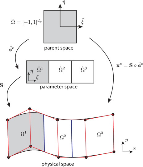
Figure 4: Diagrammatic interpretation of mappings from parent space ($\tilde{\Omega}$) through parametric space ($\hat{\Omega}$) to physical space ($\Omega$). The parent space is where numerical quadrature rules are defined.

Isogeometric analysis also makes use of an isoparametric formulation, but a key difference over its Lagrangian counterpart is the use of basis functions generated by CAD to discretise both the geometry and unknown fields. In IGA, regions bounded by knot lines with non-zero parametric area lead to a natural definition of element domains. The use of NURBS basis functions for discretisation introduces the concept of parametric space which is absent in conventional FE implementations. The consequence of this additional space is that an additional mapping must be performed to operate in parent element coordinates. As shown in Fig. 4, two mappings are considered for IGA with NURBS: a mapping $\tilde{\phi}^{e}:\tilde{\Omega}\to\hat{\Omega}^{e}$ and $\mathbf{S}:\hat{\Omega}\to\Omega$. The mapping $\mathbf{x}^{e}:\tilde{\Omega}\to\Omega^{e}$ is given by the composition $\mathbf{S}\circ\tilde{\phi}^{e}$.

For a given element $e$, the geometry is expressed as

$$\mathbf{x}^{e}(\tilde{\boldsymbol{\xi}})=\sum_{a=1}^{n_{en}}\mathbf{P}_{a}^{e}R_{a}^{e}(\tilde{\boldsymbol{\xi}})$$ (17)

where $a$ is a local basis function index, $n_{en}=(p+1)^{d_{p}}$ is the number of non-zero basis functions over element $e$ and $\mathbf{P}_{a}^{e}$,$R_{a}^{e}$ are the control point and NURBS basis function associated with index $a$ respectively. We employ the commonly used notation of an element connectivity mapping [71] which translates a local basis function index to a global index through

$$A=\textrm{IEN}(a,e)$$ (18)

Global and local control points are therefore related through $\mathbf{P}_{A}\equiv\mathbf{P}_{\textrm{IEN}(a,e)}\equiv\mathbf{P}_{a}^{e}$ with similar expressions for $R_{a}^{e}$.

Taking the case $d_{p}=d_{s}=2$, an element defined by $\hat{\Omega}^{e}=[\xi_{i},\xi_{i+1}]\otimes[\eta_{i},\eta_{i+1}]$ is mapped from parent space to parametric space through

$$\tilde{\phi}^{e}(\tilde{\boldsymbol{\xi}})=\left\{\begin{matrix}\frac{1}{2}[(\xi_{i+1}-\xi_{i})\tilde{\xi}+(\xi_{i+1}+\xi_{i})]\\ \frac{1}{2}[(\eta_{j+1}-\eta_{j})\tilde{\eta}+(\eta_{j+1}+\eta_{j})]\end{matrix}\right\}$$ (19)

A field $\mathbf{u}(\mathbf{x})$ which governs our relevant PDE can also be discretised in a similar manner to Equation (17) as

$$\mathbf{u}^{e}(\tilde{\boldsymbol{\xi}})=\sum_{a=1}^{n_{en}}\mathbf{d}_{a}^{e}R_{a}^{e}(\tilde{\boldsymbol{\xi}})$$ (20)

where $\mathbf{d}^{e}_{a}$ represents a control (nodal) variable. In contrast to conventional discretisations, these coefficients are not in general interpolatory at nodes. This is similar to the case of meshless methods built on non-interpolatory shape functions such as the moving least squares (MLS) [72, 73, 74]. Using the Bubnov-Galerkin method, an analog expansion as Equation (20) is adopted for the weight function and upon substituting them into a weak form, a standard system of linear equations is obtained from which $\mathbf{d}$–the nodal variables are obtained.

3.3 Discrete equations

The two domains $\Omega^{m}$ are discretised independently using finite elements. At the interface $\Gamma_{*}$ there is a mismatch between the two meshes, cf. Fig. 5. The approximation of the displacement field is given by

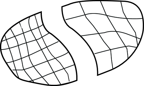
Figure 5: Independent discretisations of the domains.

$$\mathbf{u}^{m}=N_{A}^{m}\mathbf{a}_{A}^{m}$$ (21)

where $N^{m}_{A}$ denotes the finite element shape functions associated to domain $\Omega^{m}$ (which can be any Lagrange shape functions or the B-spline and NURBS basis functions presented in Section 3.1) and $\mathbf{a}_{A}^{m}=[a_{xA}^{m}\;a_{yA}^{m}\;a_{zA}^{m}]^{\mathrm{T}}$ represents the nodal displacements of domain $\Omega^{m}$.

The stresses, strains and displacements are given by

$$\boldsymbol{\sigma}^{m}=\mathbf{C}^{m}\mathbf{B}^{m}\mathbf{a}^{m},\quad\boldsymbol{\epsilon}^{m}=\mathbf{B}^{m}\mathbf{a}^{m},\quad\mathbf{u}^{m}=\mathbf{N}^{m}\mathbf{a}^{m}$$ (22)

where $\mathbf{B}$ is the standard strain-displacement matrix and $\mathbf{N}$ represents the standard shape function matrix. For two dimensional element $e$, they are given by

$$\mathbf{B}_{e}^{m}=\begin{bmatrix}N_{1,x}^{m}&0&N_{2,x}^{m}&0&\ldots\\ 0&N_{1,y}^{m}&0&N_{2,y}^{m}&\ldots\\ N_{1,y}^{m}&N_{1,x}^{m}&N_{2,y}^{m}&N_{2,x}^{m}&\ldots\end{bmatrix},\quad\mathbf{N}_{e}^{m}=\begin{bmatrix}N_{1}^{m}&0&N_{2}^{m}&0&\ldots\\ 0&N_{1}^{m}&0&N_{2}^{m}&\ldots\end{bmatrix}$$ (23)

Expressions for three dimensional elements can be found in many FEM textbooks e.g., [71]. The notation $N_{I,x}$ denotes the derivative of shape function $N_{I}$ with respect to $x$. This notation for partial derivatives will be used in subsequent sections.

The jump operator and the average operator are given by

$$\begin{split}[\![{\mathbf{u}}]\!]&=\mathbf{N}^{1}\mathbf{a}^{1}-\mathbf{N}^{2}\mathbf{a}^{2}\\ \{\boldsymbol{\sigma}\}&=\frac{1}{2}\left(\mathbf{C}^{1}\mathbf{B}^{1}\mathbf{a}^{1}+\mathbf{C}^{2}\mathbf{B}^{2}\mathbf{a}^{2}\right)\end{split}$$ (24)

and analog expansions are used for $[\![{\mathbf{w}}]\!]$ and $\{\boldsymbol{\sigma}(\mathbf{w})\}$

$$\begin{split}[\![{\mathbf{w}}]\!]&=\mathbf{N}^{1}\delta\mathbf{a}^{1}-\mathbf{N}^{2}\delta\mathbf{a}^{2}\\ \{\boldsymbol{\sigma}(\mathbf{w})\}&=\frac{1}{2}\left(\mathbf{C}^{1}\mathbf{B}^{1}\delta\mathbf{a}^{1}+\mathbf{C}^{2}\mathbf{B}^{2}\delta\mathbf{a}^{2}\right)\end{split}$$ (25)

Upon substituting Equations (22),(24) and (25) into Equation (8) and invoking the arbitrariness of $\delta\mathbf{a}^{m}$, we obtain the discrete equation that can be written as

$$\left[\mathbf{K}^{b}+\mathbf{K}^{n}+(\mathbf{K}^{n})^{\mathrm{T}}+\mathbf{K}^{s}\right]\mathbf{a}=\mathbf{f}_{\text{ext}}$$ (26)

in which $\mathbf{K}^{b}$ denotes the bulk stiffness matrix; $\mathbf{K}^{n}$ and $\mathbf{K}^{s}$ are the interfacial stiffness matrices or the coupling matrices. The external force vector is denoted by $\mathbf{f}_{\text{ext}}$ and its expression is standard and thus presented here.

The bulk stiffness matrix is given by

$$\mathbf{K}^{b}=\sum_{m}^{2}\int_{\Omega^{m}}(\mathbf{B}^{m})^{\mathrm{T}}\mathbf{C}^{m}\mathbf{B}^{m}\mathrm{d}\Omega$$ (27)

and the coupling matrices are given by

$$\mathbf{K}^{n}=\begin{bmatrix}-\displaystyle\int_{\Gamma_{*}}\mathbf{N}^{1\text{T}}\mathbf{n}\frac{1}{2}\mathbf{C}^{1}\mathbf{B}^{1}\mathrm{d}\Gamma&-\displaystyle\int_{\Gamma_{*}}\mathbf{N}^{1\text{T}}\mathbf{n}\frac{1}{2}\mathbf{C}^{2}\mathbf{B}^{2}\mathrm{d}\Gamma\\ \displaystyle\int_{\Gamma_{*}}\mathbf{N}^{2\text{T}}\mathbf{n}\frac{1}{2}\mathbf{C}^{1}\mathbf{B}^{1}\mathrm{d}\Gamma&\displaystyle\int_{\Gamma_{*}}\mathbf{N}^{2\text{T}}\mathbf{n}\frac{1}{2}\mathbf{C}^{2}\mathbf{B}^{2}\mathrm{d}\Gamma\end{bmatrix}$$ (28)

and by

$$\mathbf{K}^{s}=\begin{bmatrix}\displaystyle\int_{\Gamma_{*}}\alpha\mathbf{N}^{1\text{T}}\mathbf{N}^{1}\mathrm{d}\Gamma&-\displaystyle\int_{\Gamma_{*}}\alpha\mathbf{N}^{1\text{T}}\mathbf{N}^{2}\mathrm{d}\Gamma\\ -\displaystyle\int_{\Gamma_{*}}\alpha\mathbf{N}^{2\text{T}}\mathbf{N}^{1}\mathrm{d}\Gamma&\displaystyle\int_{\Gamma_{*}}\alpha\mathbf{N}^{2\text{T}}\mathbf{N}^{2}\mathrm{d}\Gamma\end{bmatrix}$$ (29)

If the average operator defined in Equation (7) is used, we have

$$\mathbf{K}^{n}=\begin{bmatrix}-\gamma\displaystyle\int_{\Gamma_{*}}\mathbf{N}^{1\text{T}}\mathbf{n}\mathbf{C}^{1}\mathbf{B}^{1}\mathrm{d}\Gamma&-(1-\gamma)\displaystyle\int_{\Gamma_{*}}\mathbf{N}^{1\text{T}}\mathbf{n}\mathbf{C}^{2}\mathbf{B}^{2}\mathrm{d}\Gamma\\ \gamma\displaystyle\int_{\Gamma_{*}}\mathbf{N}^{2\text{T}}\mathbf{n}\mathbf{C}^{1}\mathbf{B}^{1}\mathrm{d}\Gamma&(1-\gamma)\displaystyle\int_{\Gamma_{*}}\mathbf{N}^{2\text{T}}\mathbf{n}\mathbf{C}^{2}\mathbf{B}^{2}\mathrm{d}\Gamma\end{bmatrix}$$ (30)

4 Implementation

For the computation of the bulk stiffness matrices is standard, in this section we focus on the implementation of the coupling matrices for both two and three dimensional problems. For sake of presentation, Lagrange finite elements are discussed firstly and generalisation to NURBS elements is given subsequently with minor modifications.

4.1 Two dimensions

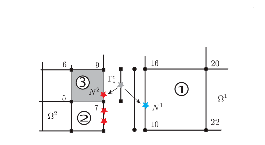
Figure 6: Independent discretisations of the domains: hierarchical meshes. The interface $\Gamma_{*}$ is discretised using the element edges of $\Omega^{2}$ that intersect $\Gamma_{*}$. For the grey element, the Gauss point is denoted by the red star which is mapped to the GP in element 1 (green star).

4.1.1 Hierarchical meshes

First, we consider hierarchical meshes as shown in Fig. 6. In this case, the interface integrals can be straightforwardly calculated as explained in what follows. Let assume that a fine mesh is adopted for $\Omega^{2}$ and a coarse mesh for $\Omega^{1}$, cf. Fig. 6. We use the fine elements on $\Gamma_{*}$ to evaluate the interfacial integral

$$\int_{\Gamma_{*}}f(N^{1},N^{2})d\Gamma=\bigcup_{e=1}^{nbe}\int_{\Gamma_{*}^{e}}f(N^{1},N^{2})d\Gamma$$ (31)

where $\Gamma_{*}^{e}=\Gamma_{*}\cap\Omega_{e}^{2,b}$ and $\{\Omega_{e}^{2,b}\}_{1}^{nbe}$ denotes elements in $\Omega^{2}$ that intersect with $\Gamma_{*}$. What makes hierarchical meshes attractive is that for a fine element on $\Gamma_{*}$ one knows the element in the coarse mesh that locates the other side of the interface.

For the elemental interface integral, a Gauss quadrature rule for line elements is adopted. For example, two GPs are used for bilinear elements. Let the GPs denoted by $\{\xi_{i}\}_{i=1}^{ngp}$. These GPs have to be mapped to two parent elements– one associated with $\Omega_{e}^{2,b}$ and one associated with $\Omega_{e}^{1,b}$. That is given $\xi_{i}$, one has to solve for $\boldsymbol{\xi}_{i}^{2}$ and $\boldsymbol{\xi}_{i}^{1}$ ($\boldsymbol{\xi}_{i}^{2}=(\xi_{i}^{2},\eta_{i}^{2})$)

$$\begin{split}\mathbf{x}_{i}&=\mathbf{M}(\xi_{i})\mathbf{x}_{l}\\ \mathbf{x}_{i}&=\mathbf{N}^{2}(\boldsymbol{\xi}_{i}^{2})\mathbf{x}_{e}^{2}\rightarrow\boldsymbol{\xi}_{i}^{2}\\ \mathbf{x}_{i}&=\mathbf{N}^{1}(\boldsymbol{\xi}_{i}^{1})\mathbf{x}_{e}^{1}\rightarrow\boldsymbol{\xi}_{i}^{1}\end{split}$$ (32)

where the first equation is used to compute the global coordinates of the GP ($\mathbf{x}_{i}=(x_{i},y_{i})$) and the second and third equations are used to compute the natural coordinates of the GP in the parent element associated with $\Omega_{e}^{k,b}$. Usually a Newton-Raphson method is used for this. In the above, $\mathbf{M}$ denotes the row vector of shape functions of a two-noded line element; $\mathbf{x}_{l}$ are the nodal coordinates of two boundary nodes of $\Gamma_{*}^{e}$ (for the example given in Fig. 6, they are nodes 7 and 9); $\mathbf{x}_{e}^{k}$ ($k=1,2$) denotes the nodal coordinates of $\Omega_{e}^{k,b}$. $\mathbf{N}^{k}$ denote the row vector of shape functions of element $\Omega_{e}^{k,b}$. For the example given in Fig. 6, $\mathbf{x}_{e}^{2}$ stores the coordinates of nodes 5,7,9 and 6. And, $\mathbf{x}_{e}^{1}$ stores the coordinates of nodes 10,22,20 and 16.

It is now ready to evaluate the interfacial integral as

$$\int_{\Gamma_{*}^{e}}f(N^{1},N^{2})\mathrm{d}\Gamma=\sum_{i=1}^{ngp}f(N^{1}(\boldsymbol{\xi}_{i}^{1}),N^{2}(\boldsymbol{\xi}_{i}^{2}))w_{i}$$ (33)

where $w_{i}$ equals the weight multiplied with the Jacobian of the transformation from the line parent element $[-1,1]$ to $\Gamma_{*}^{e}$.

Finally the coupling terms are assembled to the global stiffness matrix in a standard manner. For example $\mathbf{K}^{n,11}$ is assembled using the connectivity of $\Omega_{e}^{1,b}$ and $\mathbf{K}^{n,22}$ is assembled using the connectivity of $\Omega_{e}^{2,b}$.

4.1.2 Non-matching structured meshes

Non-matching structured meshes are plotted in Fig. 7. In those cases, the evaluation of the interfacial integrals are more complicated. We use the trace mesh of $\Omega^{1}$ on the coupling interface $\Gamma_{*}$ to perform the numerical integration. We use two data structures to store the Gauss points namely (for the concrete example shown in Fig. 7) $gp1=\{(\boldsymbol{\xi}^{1}_{i},w_{i},e^{1}_{i})\}_{i=1}^{4}$ and $gp2=\{(\boldsymbol{\xi}^{2}_{i},e^{2}_{i})\}_{i=1}^{4}$ where $e^{m}_{i}$ indicates the index of element of $\Omega^{m}$ that contains GP $\boldsymbol{\xi}^{m}_{i}$. After having these GPs, the assembly of the coupling matrices follows the procedure outlined in Box 1.

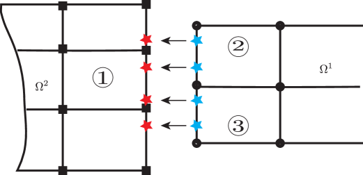
Figure 7: Independent discretisations of the domains: non-matching structured meshes.

Box 1 Assembly of coupling matrices

1. Loop over Gauss points (GPs), $i$

   1. Get $\boldsymbol{\xi}^{1}_{i}$, $w_{i}$ and $e^{1}_{i}$ from $gp1$

   2. Get $\boldsymbol{\xi}^{2}_{i}$ and $e^{2}_{i}$ from $gp2$

   3. Compute shape functions $\mathbf{N}^{1}(\boldsymbol{\xi}^{1}_{i})$

   4. Compute shape functions $\mathbf{N}^{2}(\boldsymbol{\xi}^{2}_{i})$

   5. Compute $\mathbf{K}^{s,12}=-\alpha\mathbf{N}^{1\text{T}}\mathbf{N}^{2}w_{i}$

   6. Assemble $\mathbf{K}^{s,12}$ to the global stiffness matrix using the connectivity array of $e^{1}_{i}$ (rows) and $e^{2}_{i}$ (columns).

2. End loop over GPs

4.2 Three dimensional formulations

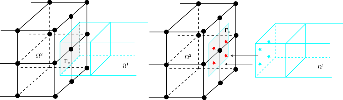
Figure 8: Coupling of two three dimensional continuum models. For evaluating the coupling terms, we use the trace mesh of $\Omega^{1}$ on the coupling interface $\Gamma_{*}$. In this figure, there is only one element of the trace mesh for sake of illustration.

This section presents the implementation for 3D, we refer to Fig. 8. The computation of GPs required for the coupling matrices is given in Box 2. After having obtained $gp1$ and $gp2$ data structures, the assembly of the coupling matrices follows Box 1.

Box 2 Determination of $gp1$ and $gp2$

1. For each element $e^{1}$ of the trace mesh, do

   1. Distribute GPs on the face, $\{(\xi_{i},\eta_{i},w_{i})\}_{i=1}^{ngp}$

   2. Loop over the GPs, $i$

      1. Transform GP $i$ to physical space using

         $$\mathbf{x}_{i}=\mathbf{M}(\xi_{i},\eta_{i})\mathbf{x}_{l}$$ (34)

      2. Compute tangent vectors, normal vector and the weight

         $$\mathbf{a}_{1}=\mathbf{M}_{,\xi}\mathbf{x}_{l},\quad\mathbf{a}_{2}=\mathbf{M}_{,\eta}\mathbf{x}_{l},\quad\mathbf{n}=\frac{\mathbf{a}_{1}\times\mathbf{a}_{2}}{\left|\left|\mathbf{a}_{1}\times\mathbf{a}_{2}\right|\right|},\quad\bar{w}_{i}=w_{i}\left|\left|\mathbf{a}_{1}\times\mathbf{a}_{2}\right|\right|$$ (35)

      3. Transform GP $i$ from physical space to parent space of $\Omega^{1}$ using

         $$\mathbf{x}_{i}=\mathbf{N}^{1}(\xi_{i}^{1},\eta_{i}^{1},\zeta_{i}^{1})\mathbf{x}_{e}^{1}\rightarrow(\xi_{i}^{1},\eta_{i}^{1},\zeta_{i}^{1})$$ (36)

      4. Find index of element in $\Omega^{2}$ that contains $\mathbf{x}_{i}$, named it $e^{2}$

      5. Transform GP $i$ from physical space to parent space of $\Omega^{2}$ using

         $$\mathbf{x}_{i}=\mathbf{N}^{2}(\xi_{i}^{2},\eta_{i}^{2},\zeta_{i}^{2})\mathbf{x}_{e}^{2}\rightarrow(\xi_{i}^{2},\eta_{i}^{2},\zeta_{i}^{2})$$ (37)

         where $\mathbf{x}_{e}^{2}$ are the nodal coordinates of element $e^{2}$.

   3. End loop over GPs

2. End for

4.3 Extension to NURBS elements

Since NURBS basis functions are defined on the parameter space not on the parent space, there is a slight modification to the implementation. The GPs are now give by $\{(\tilde{\xi}_{i},\tilde{\eta}_{i},\tilde{w}_{i})\}_{i=1}^{ngp}$. They are firstly transformed to the parameter space using the mapping defined in Equation (19): $\{(\xi_{i},\eta_{i},w_{i})\}_{i=1}^{ngp}$ where $w_{i}=\tilde{w}_{i}J$ with $J$ is the Jacobian of the parent-to-parameter mapping. After that one works with the parameter space, for example the inverse mapping Equation (36) determines a point in the parameter space.

Steps (iv) and (v) in the algorithm given in Box 2 demand modifications because one can exploit the fact that the NURBS mapping, Equation (16), is global. Hence, one writes Equation (37) as follows

$$\mathbf{x}_{i}=\mathbf{N}^{2}(\xi_{i}^{2},\eta_{i}^{2},\zeta_{i}^{2})\mathbf{x}^{2}\rightarrow(\xi_{i}^{2},\eta_{i}^{2},\zeta_{i}^{2})$$ (38)

where $\mathbf{x}^{2}$ are the control point of patch 2. Note that in Equation (36), $\mathbf{x}^{1}_{e}$ denotes the control points of only the element under consideration. Using the output $(\xi_{i}^{2},\eta_{i}^{2},\zeta_{i}^{2})$ and the standard $FindSpan$ algorithm, cf. [1], one can determine which element $\mathbf{x}_{i}$ belongs to i.e., $e^{2}$.

Remark 4.1.

Note also that if Bézier extraction is used to implement NURBS-based IGA, see e.g., [75], then this section can be ignored since with Bézier extraction the basis are the Bernstein basis, which are defined in the parent space as well, multiplied with some sparse matrices. Moreover, Bézier extraction will facilitate the incorporation of the non-conforming multi-patch NURBS IGA into existing FE codes including commercially available FE packages.

5 Numerical examples

In this section three numerical examples of increasing complexity are presented to assess the performance of the proposed method. They are listed as follows

1. Timoshenko beam (2D/2D coupling)

2. Cantilever beam (3D/3D coupling)

3. Connecting rod (complex 3D/3D coupling)

The first two examples are simple problems to verify the implementation and we provide convergence analysis for the first example. Unless otherwise stated, we use MIGFEM–an open source Matlab IGA code which is available at https://sourceforge.net/projects/cmcodes/ for our computations and the visualisation was performed in Paraview [76].

5.1 Timoshenko beam

Consider a beam of dimensions $L\times D$ (unit thickness), subjected to a parabolic traction at the free end as shown in Fig. 9. A plane stress state is assumed. The parabolic traction is given by

$$t_{y}(y)=-\frac{P}{2I}\biggl{(}\frac{D^{2}}{4}-y^{2}\biggr{)}$$ (39)

where $I=D^{3}/12$ is the moment of inertia. The exact displacement field of this problem is, see e.g., [77]

$$\begin{split}u_{x}(x,y)&=\frac{Py}{6EI}\biggl{[}(6L-3x)x+(2+\nu)\biggl{(}y^{2}-\frac{D^{2}}{4}\biggr{)}\biggr{]}\\ u_{y}(x,y)&=-\frac{P}{6EI}\biggl{[}3\nu y^{2}(L-x)+(4+5\nu)\frac{D^{2}x}{4}+(3L-x)x^{2}\biggr{]}\\ \end{split}$$ (40)

and the exact stresses are

$$\sigma_{xx}(x,y)=\frac{P(L-x)y}{I};\quad\sigma_{yy}(x,y)=0,\quad\sigma_{xy}(x,y)=-\frac{P}{2I}\biggl{(}\frac{D^{2}}{4}-y^{2}\biggr{)}$$ (41)

In the computations, material properties are taken as $E=3.0\times 10^{7}$, $\nu=0.3$ and the beam dimensions are $D=6$ and $L=48$. The shear force is $P=1000$. In order to model the clamping condition, the displacement defined by Equation (40) is prescribed as essential boundary conditions at $x=0,-D/2\leq y\leq D/2$. This problem is solved with bilinear Lagrange elements and high order B-splines elements. The former helps to verify the implementation in addition to the ease of enforcement of Dirichlet boundary conditions (BCs). For the latter, care must be taken in enforcing the Dirichlet BCs given in Equation (40) since the B-splines are not interpolatory. The beam is divided into two domains by a vertical line at $x=L/2$ i.e., $\Gamma^{*}=\{x=L/2,-D/2\leq y\leq D/2\}$.

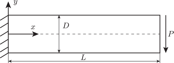
Figure 9: Timoshenko beam: problem description.

Lagrange elements Firstly, a conforming mesh (however there are double nodes at $\Gamma^{*}$) is considered and each domain is discretised by a mesh of $20\times 4$ elements as given in Fig. 10a. Then, a non-conforming mesh where the left domain is discretised by $20\times 8$ elements and the right domain is meshed by $20\times 4$ is considered, cf. Fig. 10b. A value of $1\times 10^{8}$ was used for $\alpha$. The vertical displacements along the midline of the beam ($u_{y}(0\leq x\leq L,y=0$) are plotted in Fig. 11 together with the exact solution. A good agreement can be observed. The stresses are plotted in Fig. 12.

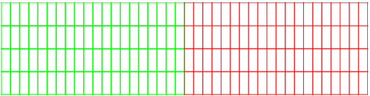
(a) Conforming mesh

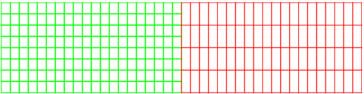
(b) Non conforming mesh

Figure 10: Timoshenko beam: conforming and non-conforming meshes. Note that even with the conforming mesh, there are double nodes at the coupling interface $x=L/2,-D/2\leq y\leq D/2$.

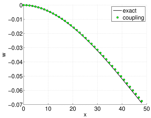
(a) Conforming mesh

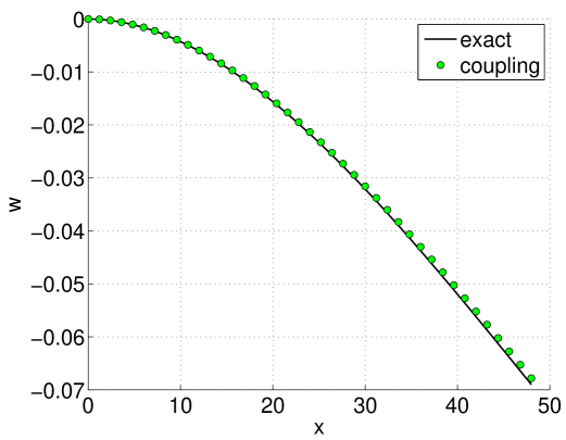
(b) Non-conforming mesh

Figure 11: Timoshenko beam: comparison of $u_{y}(0\leq x\leq L,y=0)$ with the exact solution.

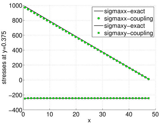
(a) Stresses along the beam length

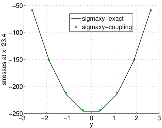
(b) Stresses over the beam height

Figure 12: Timoshenko beam: stresses obtained with a conforming mesh ($20\times 8$ for each domain).

B-splines elements Next, we study the performance of the B-splines elements of which one mesh is given in Fig. 13. Dirichlet BCs are enforced using the least square projection method see e.g., [78]. Note that Nitche’s method can also be used to weakly enforce the Dirichlet BCs. However, we use Nitsche’s method only to couple the patch interfaces. As detailed in [71] for Lagrangian basis functions, a rule of $(p+1)\times(q+1)$ Gaussian quadrature can be applied for two-dimensional elements in which $p$ and $q$ denote the orders of the chosen basis functions in the $\xi$ and $\eta$ direction. The same procedure is also used for NURBS basis functions in the present work, although it should be emphasised that Gaussian quadrature is not optimal for IGA [79, 80]. The stresses are given in Fig. 14.

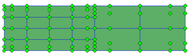
Figure 13: Timoshenko beam: B-spline bi-cubic ($p=q=3$) mesh with $4\times 4$ elements for the left domain and $2\times 2$ elements for the right one. The filled circles denote the control points.

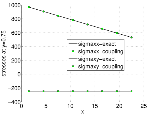
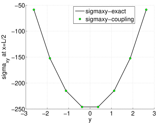
Figure 14: Timoshenko beam: stresses with B-splines elements. The left domain is meshed by $8\times 8$ cubic elements and the right domain with $2\times 2$ cubic elements.

Finally we present results obtained with a non-hierarchical B-spline mesh as given in Fig. 15: a $8\times 6$ bi-cubic mesh is used for the left domain and a bi-cubic $4\times 3$ mesh is used for the right domain. A quadratic stress profile was obtained where the theoretical maximum value along the midline of the beam (250) can be observed.

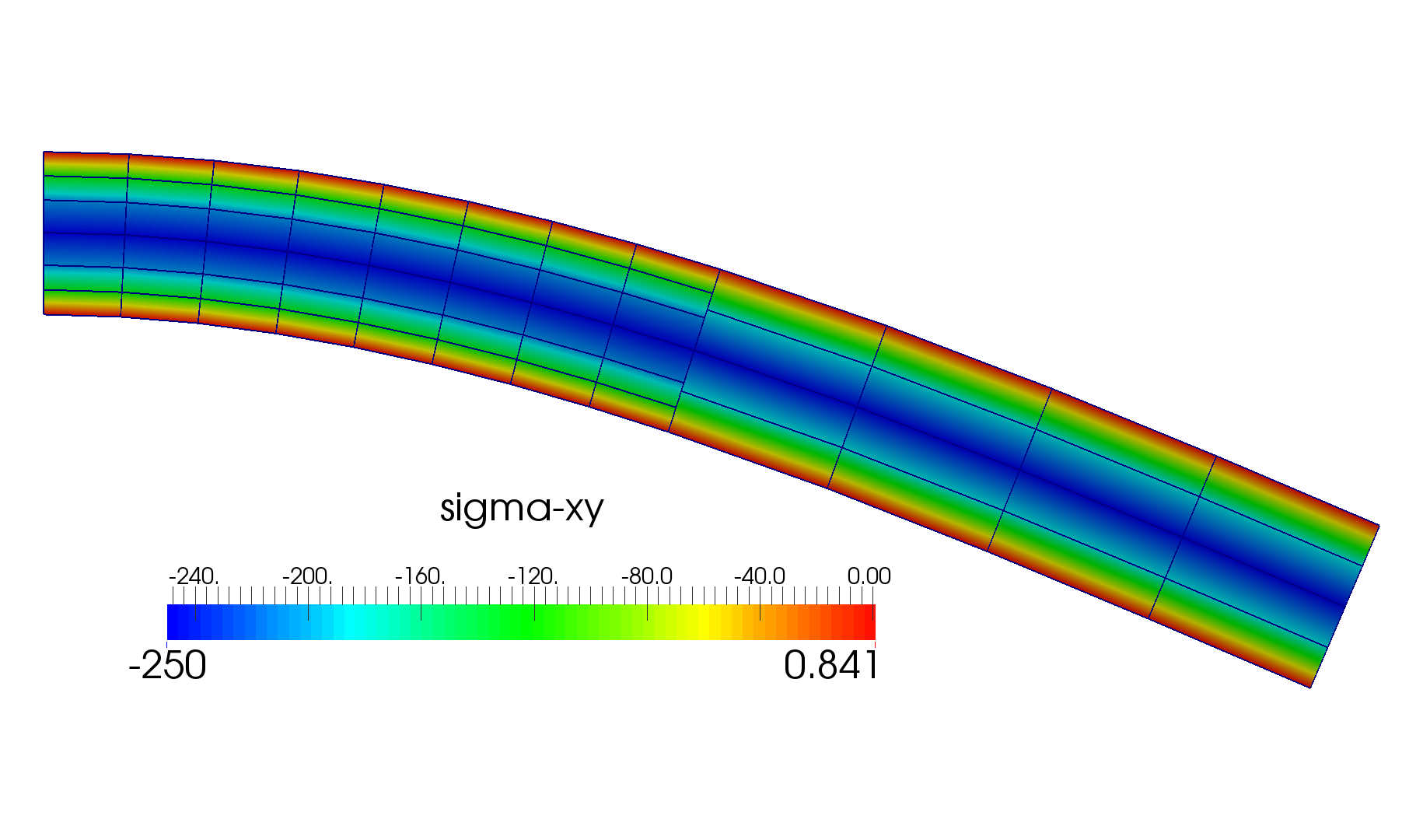
Figure 15: Timoshenko beam: non-hierarchical B-spline mesh ($8\times 6$ cubic elements for the left domain and $4\times 3$ cubic elements for the right domain).

Convergence study In order to assess the convergence of the method, displacement and energy norms are evaluated with the energy norm given by

$$e_{\text{energy}}=\left[\frac{1}{2}\int_{\Omega}\left(\boldsymbol{\varepsilon}_{\mathrm{num}}-\boldsymbol{\varepsilon}_{\mathrm{exact}}\right)\cdot\mathbf{D}\cdot\left(\boldsymbol{\varepsilon}_{\mathrm{num}}-\boldsymbol{\varepsilon}_{\mathrm{exact}}\right)\mathrm{d}\Omega\right]^{\frac{1}{2}},$$ (42)

and the displacement norm defined as

$$e_{\text{displacement}}=\left\{{\displaystyle\int_{\Omega}\left[\left({\bf u}_{\text{num}}-{\bf u}_{\text{exact}}\right)\cdot\left({\bf u}_{\text{num}}-{\bf u}_{\text{exact}}\right)\right]\mathrm{d}\Omega}\right\}^{1/2},$$ (43)

where $\boldsymbol{\varepsilon}_{\mathrm{num}}$, and $\boldsymbol{\varepsilon}_{\mathrm{exact}}$ are the numerical strain vector and exact strain vector, respectively. The same notation applies to the displacement vector ${\bf u}_{\text{num}}$ and ${\bf u}_{\text{exact}}$. In the post-processing step, the above norms are calculated using the same Gauss-Legendre quadrature that has been adopted for the stiffness matrix computation.

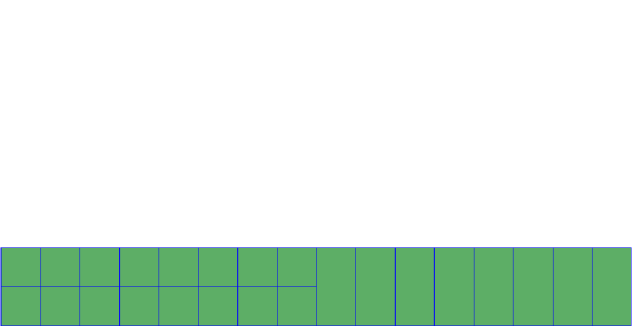
Figure 16: Convergence study of the Timoshenko beam: initial mesh from which refined meshes are obtained by dividing each knot span into two equal halves.

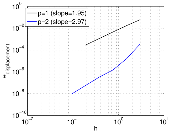
(a) displacement norm

(b) energy norm

Figure 17: Timoshenko beam: convergence plots.

The initial mesh from which refined meshes were obtained is given in Fig. 16. It can be shown that for linear elasticity $\alpha$ depends on the element size $h_{e}$ and the material parameters, see for example [81, 65]

$$\alpha=\frac{\lambda+\mu}{2}\frac{\theta(p)}{h_{e}}$$ (44)

where $\theta(p)$ is a positive number that depends only on the polynomial order $p$ of the finite element approximation. For bilinear basis functions, we set $\theta(p=1)=12$ and for bi-quadratic basis functions, we set $\theta(p=2)=36$. These values were chosen so that the stiffness matrix is positive definite. Thus, for each mesh, Equation (44) was used to compute the stabilisation parameter. The convergence plots are given in Fig. 17 where optimal convergence rates for both displacement and energy norms were obtained. Note that minimum values of $\alpha$ can be computed based on a numerical analysis of the discrete forms and lead to the global [69] and local generalized eigenvalue approaches [64].

5.2 Plate with a center inclusion

Consider a plate with a center inclusion as given in Fig. 18. The matrix properties are denoted by $E_{m}$ and $\nu_{m}$ and the inclusion properties are denoted by $E_{i}$ and $\nu_{i}$. A traction along the vertical direction is applied on the top edge while nodes along the bottom edge are constrained. This problem is solved with (1) embedded Nitsche’s method and (2) XFEM which are methods that do not require a mesh conforming to the inclusion. The XFEM mesh is given in Fig. 19a where $30\times 60$ four-noded quadrilateral (Q4) elements are adopted. The material interface is modeled via enrichment functions (the $abs$ enrichment function) proposed in [82]. Meshes in the Nitsche’s method, cf. Fig. 19b, consist of a background mesh for the plate ($32\times 64$ Q4 elements) and another mesh for the inclusion which is embedded in the background mesh ($16\times 16$ bi-quadratic NURBS elements).

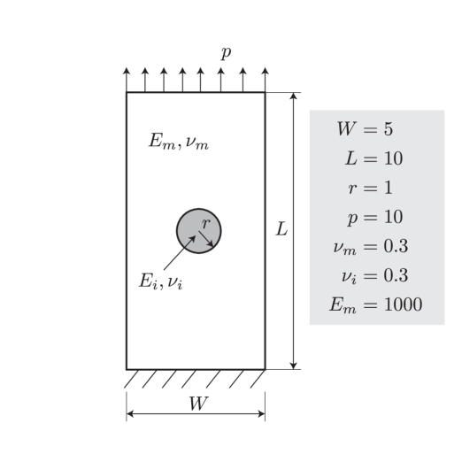
Figure 18: A plate with a center inclusion.

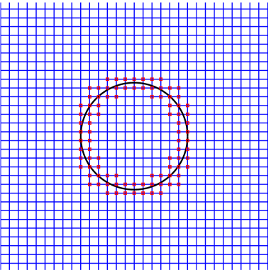
(a) XFEM

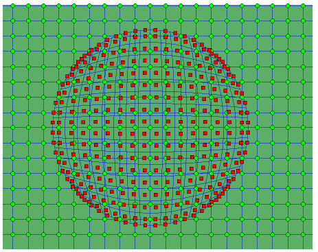
(b) Nitsche

Figure 19: Plate with a center inclusion: (a) XFEM mesh with enriched nodes and (b) Nitsche’s method with embedded mesh.

For details on the Nitsche based embedded mesh method, we refer to e.g., [60]. Here, we apply this method in the context of IGA by using NURBS elements. The implementation is briefly explained as follows. The assembly of inclusion elements is standard and the assembly of background elements is similar to XFEM for voids–void elements (completely covered by inclusion elements) do not contribute to the total stiffness matrix, cut elements (elements cut by the inclusion) require special integration scheme in which the part falls within the inclusion domain is not integrated. This can be achieved using the standard sub-triangulation technique in the context of XFEM [42] or the hierarchical element subdivision employed in the Finite Cell Method [66] or the technique used in the NEFEM (NURBS Enhanced FEM) [83]. Here, for simplicity, we used the hierarchical element subdivision method. We refer to Fig. 20. The inclusion Young’s modulus is $E_{i}=1$. Due to the contrast in Young’s moduli, the average operator given in Equation (7) was used with $\gamma=E_{m}/(E_{m}+E_{i})$ as proposed in [60]. The stabilisation parameter is chosen empirically $\alpha=1e6$. Fig. 21 shows the contour plot of $u_{y}$ solutions obtained with both methods. A good agreement of Nitsche solution compared with XFEM solution can be observed.

Figure 20: A plate with a center inclusion: Nitsche based embedded mesh method. The red filled squares denote Gauss points to evaluate the coupling matrices. Cyan squares denote void elements and red squares represent cut elements.

Figure 21: A plate with a center inclusion: contour plot of $u_{y}$ solutions–xfem (left) and Nitsche (right).

5.3 3D-3D coupling

In order to test the implementation for 3D problems, we consider the 3D cantilever beam shown in Fig. 22. The data are: Young’s modulus $E=1000$, Poisson’s ratio $\nu=0.3$, $L=10$, $W=H=1$ and the imposed displacement in the $z$-direction is $1$. The non-conforming B-splines discretisation is given in Fig. 23 where the beam is divided into two equal parts. A value of … was used for the stabilisation parameter $\alpha$. In Fig. 24 the contour plot of $\sigma_{xx}$ is given and a comparison was made with a standard Galerkin discretisation of $32\times 4\times 4$ tri-cubic B-splines elements and a good agreement was obtained.

Figure 22: A 3D cantilever beam subjected to an imposed vertical displacement.

Figure 23: A 3D cantilever beam subjected to an imposed vertical displacement: $16\times 4\times 4$ tri-cubic B-splines elements for the left domain and $16\times 1\times 2$ tri-cubic B-splines elements for the right domain.

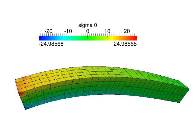
(a) Nitsche

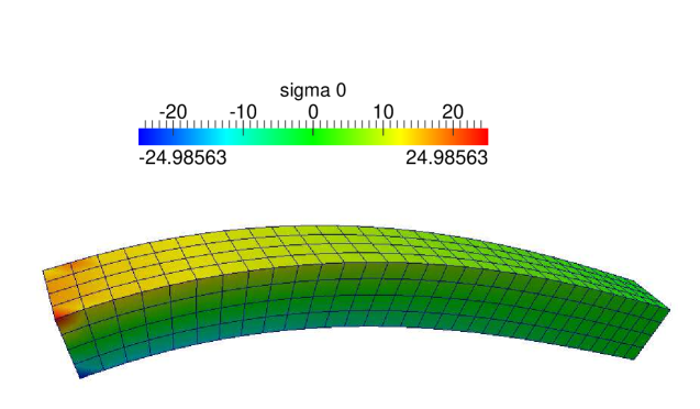
(b) Galerkin

Figure 24: Timoshenko beam.

5.4 Connecting rod

The method is now applied to a more complicated geometry, taking into account more than one interface coupling, curved interfaces and interfaces with different dimension. This geometry is a simplified representation of a connecting rod, which is a component of an internal combustion engine, and represents a classic linear case in the stress-strain static analysis. The geometric input model is composed by three NURBS patches (see Fig. 1) with two coupling interfaces. The dimensions are consistent with an actual component and the material properties are Young’s modulus $E=2\times 10^{5}$ MPa, Poisson’s ratio $\nu=0.3$ which come from a standard steel material. Boundary conditions are represented in Fig. 25: ideal fixed boundary condition on the two vertical surfaces of the (big-end) and a vertical total force $F=1000$ N load applied to the internal ring of the small-end, according to the effect of the pin-piston sub-assembly that transmits a bending moment to the connecting-rod stem. For the simulation the model is refined with tri-cubic functions and $32\times 4\times 8$ elements for patch 1, $24\times 12\times 4$ elements for patch 2 and $64\times 4\times 8$ elements for patch 3, resulting in a total number of 4224 elements and 11305 control points. For both coupling interfaces the smaller faces are the regions where the surface integration is performed and a stabilization parameter $\alpha=1\times 10^{8}$ was chosen empirically. The results are shown in Fig. 26, where displacement and stress fields are plotted. The displacement distribution is the typical progressive cubic polynomial form of the analytical Saint-Venant model. The pattern distribution of the Von Mises equivalent failure criterion is used for the comparison of the simulation results in IGA approach with respect to Siemens-NX (traditional FE model, discretized with second order tetrahedra, 6182 elements and 11332 nodes Fig. 27). Typical combined compressive and bending stress/action of the connecting-rod stem is representable with Von Mises stresses closed to zero in the mean plane; superior fibres has the maximum value of traction symmetrically equivalent to the compression of inferior fibres, due to the strictly positive equivalent measure of Von Mises yield criterion. In both analyses interesting three-dimensional effects are detected: maximum stress values correspond to the free fibres of the stem in superior and inferior surfaces that interact with the big-end; the interaction between the stem and both the big-end and small-end produces an increasing stress value in the azure region in proximity of the neutral axis that is very well described in both analysis, thus demonstrating the IGA model effectiveness of the links between patches; the boundary conditions are typically hyperstatic and only the inner part of the big-end transmits traction/compression reactions (green regions); due to this particular load case, parts of the big-end (blue regions) are superfluous in both analyses and could be deleted, reducing the mass of the component; the internal stress distribution in the inner ring of the small-end shows again very good agreement of the combined compressive and bending stress/action behaviour that reaches the pin region.

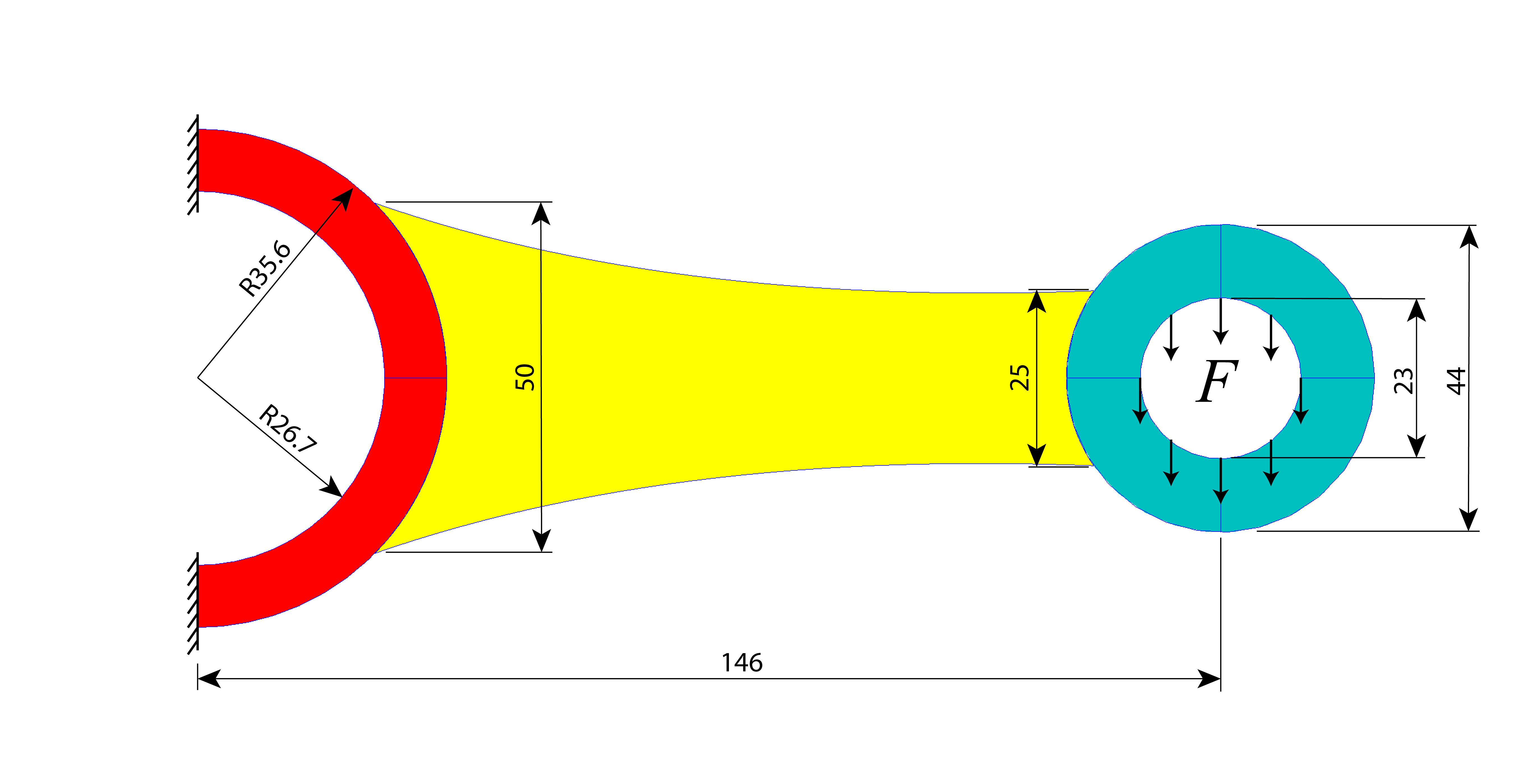
Figure 25: Connecting-rod: geometry and boundary conditions. The dimensions are in mm.

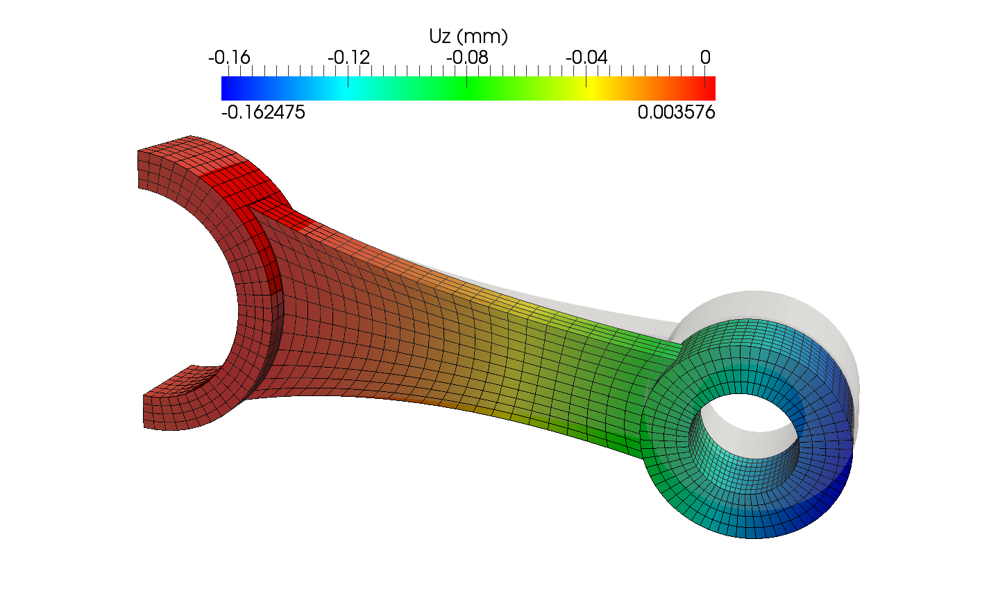
(a) z-displacement field

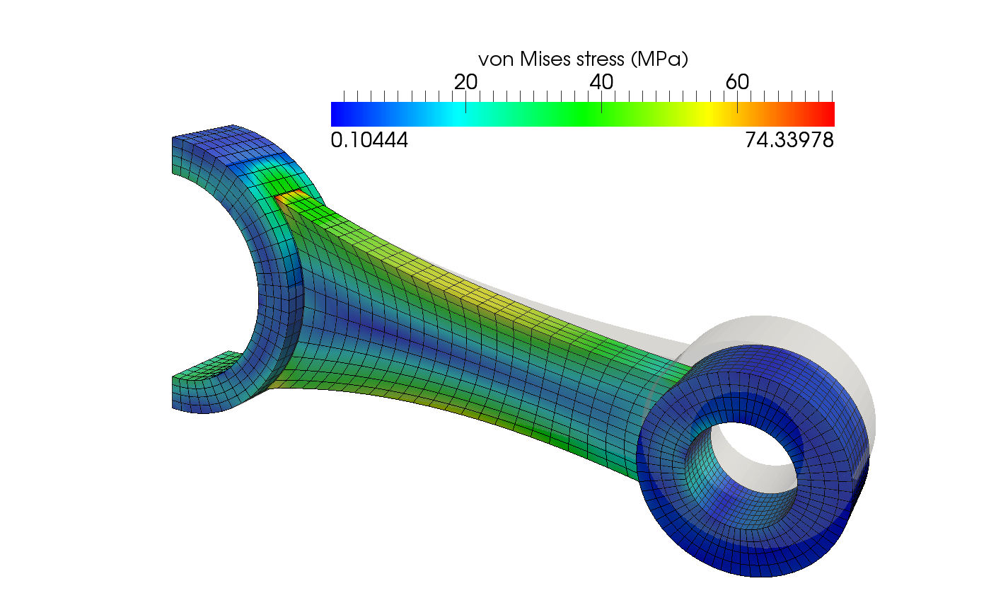
(b) Stress field

Figure 26: Results of the connecting rod.

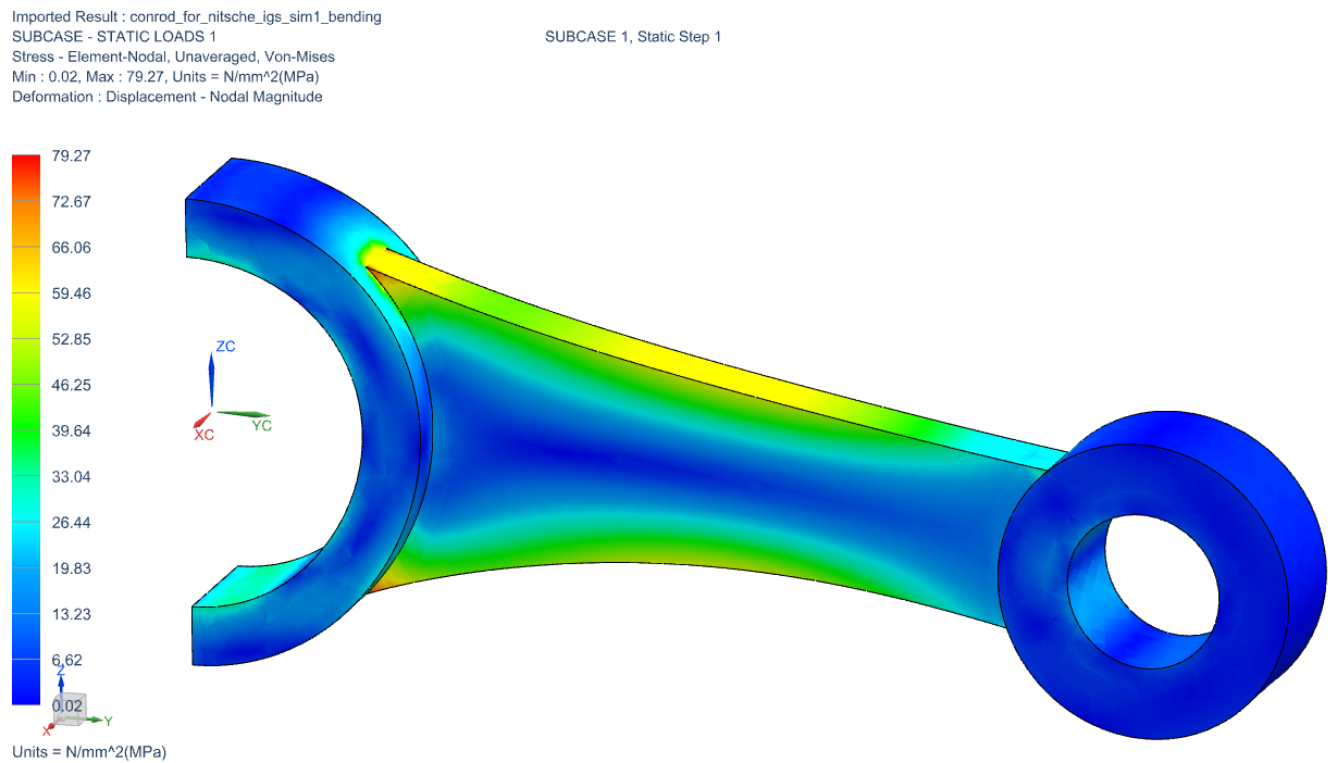
Figure 27: Stress plot from the commercial code NX-NASTRAN.

6 Conclusions

We presented a Nitsche’s method to couple non-conforming NURBS patches. Detailed implementation was provided and numerical examples demonstrated the good performance of the method. The proposed method certainly enlarges the applicability of NURBS based isogeometric analysis.

The contribution was limited to linear elastostatic problems and extension of the method to (1) dynamics problems and (2) nonlinear material problems is under investigation before one could claim whether Nitsche coupling would be a viable method for multi-patch NURBS based isogeometric analysis.

As we were preparing the paper for submission, we became aware of contemporary work had been presented the previous week at the US National Congress for Computational Mechanics [84] in the context of the finite cell method.

References

- [1] L. A. Piegl and W. Tiller. The NURBS Book. Springer, 1996.
- [2] D. F. Rogers. An Introduction to NURBS with Historical Perspective. Academic Press, 2001.
- [3] T.J.R. Hughes, J.A. Cottrell, and Y. Bazilevs. Isogeometric analysis: CAD, finite elements, NURBS, exact geometry and mesh refinement. Computer Methods in Applied Mechanics and Engineering, 194(39-41):4135–4195, 2005.
- [4] J. A. Cottrell, T. J.R. Hughes, and Y. Bazilevs. Isogeometric Analysis: Toward Integration of CAD and FEA. Wiley, 2009.
- [5] P. Kagan, A. Fischer, and P. Z. Bar-Yoseph. New B-Spline Finite Element approach for geometrical design and mechanical analysis. International Journal for Numerical Methods in Engineering, 41(3):435–458, 1998.
- [6] P. Kagan and A. Fischer. Integrated mechanically based CAE system using B-Spline finite elements. Computer-Aided Design, 32(8–9):539 – 552, 2000.
- [7] F. Cirak, M. Ortiz, and P. Schröder. Subdivision surfaces: a new paradigm for thin-shell finite-element analysis. International Journal for Numerical Methods in Engineering, 47(12):2039–2072, 2000.
- [8] D.J. Benson, Y. Bazilevs, M.C. Hsu, and T.J.R. Hughes. Isogeometric shell analysis: The Reissner–Mindlin shell. Computer Methods in Applied Mechanics and Engineering, 199(5-8):276–289, 2010.
- [9] J. Kiendl, K.-U. Bletzinger, J. Linhard, and R. Wüchner. Isogeometric shell analysis with Kirchhoff-Love elements. Computer Methods in Applied Mechanics and Engineering, 198(49-52):3902–3914, 2009.
- [10] D.J. Benson, Y. Bazilevs, M.-C. Hsu, and T.J.R. Hughes. A large deformation, rotation-free, isogeometric shell. Computer Methods in Applied Mechanics and Engineering, 200(13-16):1367–1378, 2011.
- [11] L. Beirão da Veiga, A. Buffa, C. Lovadina, M. Martinelli, and G. Sangalli. An isogeometric method for the Reissner-Mindlin plate bending problem. Computer Methods in Applied Mechanics and Engineering, 209–212:45–53, 2012.
- [12] T. K. Uhm and S. K. Youn. T-spline finite element method for the analysis of shell structures. International Journal for Numerical Methods in Engineering, 80(4):507–536, 2009.
- [13] R. Echter, B. Oesterle, and M. Bischoff. A hierarchic family of isogeometric shell finite elements. Computer Methods in Applied Mechanics and Engineering, 254:170 – 180, 2013.
- [14] D.J. Benson, S. Hartmann, Y. Bazilevs, M.-C. Hsu, and T.J.R. Hughes. Blended isogeometric shells. Computer Methods in Applied Mechanics and Engineering, 255:133 – 146, 2013.
- [15] J. Kiendl, Y. Bazilevs, M.-C. Hsu, R. Wüchner, and K.-U. Bletzinger. The bending strip method for isogeometric analysis of Kirchhoff-Love shell structures comprised of multiple patches. Computer Methods in Applied Mechanics and Engineering, 199(37-40):2403–2416, 2010.
- [16] İ. Temizer, P. Wriggers, and T.J.R. Hughes. Contact treatment in isogeometric analysis with NURBS. Computer Methods in Applied Mechanics and Engineering, 200(9-12):1100–1112, 2011.
- [17] L. Jia. Isogeometric contact analysis: Geometric basis and formulation for frictionless contact. Computer Methods in Applied Mechanics and Engineering, 200(5-8):726–741, 2011.
- [18] İ. Temizer, P. Wriggers, and T.J.R. Hughes. Three-Dimensional Mortar-Based frictional contact treatment in isogeometric analysis with NURBS. Computer Methods in Applied Mechanics and Engineering, 209–212:115–128, 2012.
- [19] L. De Lorenzis, İ. Temizer, P. Wriggers, and G. Zavarise. A large deformation frictional contact formulation using NURBS-bases isogeometric analysis. International Journal for Numerical Methods in Engineering, 87(13):1278–1300, 2011.
- [20] M.E. Matzen, T. Cichosz, and M. Bischoff. A point to segment contact formulation for isogeometric, NURBS based finite elements. Computer Methods in Applied Mechanics and Engineering, 255:27 – 39, 2013.
- [21] W. A. Wall, M. A. Frenzel, and C. Cyron. Isogeometric structural shape optimization. Computer Methods in Applied Mechanics and Engineering, 197(33-40):2976–2988, 2008.
- [22] N. D. Manh, A. Evgrafov, A. R. Gersborg, and J. Gravesen. Isogeometric shape optimization of vibrating membranes. Computer Methods in Applied Mechanics and Engineering, 200(13-16):1343–1353, 2011.
- [23] X. Qian and O. Sigmund. Isogeometric shape optimization of photonic crystals via Coons patches. Computer Methods in Applied Mechanics and Engineering, 200(25-28):2237–2255, 2011.
- [24] X. Qian. Full analytical sensitivities in NURBS based isogeometric shape optimization. Computer Methods in Applied Mechanics and Engineering, 199(29-32):2059–2071, 2010.
- [25] R.N. Simpson, S.P.A. Bordas, J. Trevelyan, and T. Rabczuk. A two-dimensional isogeometric boundary element method for elastostatic analysis. Computer Methods in Applied Mechanics and Engineering, 209–212:87–100, 2012.
- [26] M.A. Scott, R.N. Simpson, J.A. Evans, S. Lipton, S.P.A. Bordas, T.J.R. Hughes, and T.W. Sederberg. Isogeometric boundary element analysis using unstructured T-splines. Computer Methods in Applied Mechanics and Engineering, 254:197 – 221, 2013.
- [27] H. Gomez, T.J.R. Hughes, X. Nogueira, and V. M. Calo. Isogeometric analysis of the isothermal Navier-Stokes-Korteweg equations. Computer Methods in Applied Mechanics and Engineering, 199(25-28):1828–1840, 2010.
- [28] P. N. Nielsen, A. R. Gersborg, J. Gravesen, and N. L. Pedersen. Discretizations in isogeometric analysis of Navier-Stokes flow. Computer Methods in Applied Mechanics and Engineering, 200(45-46):3242–3253, 2011.
- [29] Y. Bazilevs and I. Akkerman. Large eddy simulation of turbulent Taylor-Couette flow using isogeometric analysis and the residual-based variational multiscale method. Journal of Computational Physics, 229(9):3402–3414, 2010.
- [30] Y. Bazilevs, V. M. Calo, T. J. R. Hughes, and Y. Zhang. Isogeometric fluid-structure interaction: theory, algorithms, and computations. Computational Mechanics, 43:3–37, 2008.
- [31] Y. Bazilevs, J.R. Gohean, T.J.R. Hughes, R.D. Moser, and Y. Zhang. Patient-specific isogeometric fluid-structure interaction analysis of thoracic aortic blood flow due to implantation of the Jarvik 2000 left ventricular assist device. Computer Methods in Applied Mechanics and Engineering, 198(45-46):3534–3550, 2009.
- [32] H. Gómez, V. M. Calo, Y. Bazilevs, and T.J.R. Hughes. Isogeometric analysis of the Cahn-Hilliard phase-field model. Computer Methods in Applied Mechanics and Engineering, 197(49-50):4333–4352, 2008.
- [33] C. V. Verhoosel, M. A. Scott, T. J. R. Hughes, and R. de Borst. An isogeometric analysis approach to gradient damage models. International Journal for Numerical Methods in Engineering, 86(1):115–134, 2011.
- [34] P. Fischer, M. Klassen, J. Mergheim, P. Steinmann, and R. Müller. Isogeometric analysis of 2D gradient elasticity. Computational Mechanics, 47:325–334, 2010.
- [35] A. Masud and R. Kannan. B-splines and NURBS based finite element methods for Kohn-Sham equations. Computer Methods in Applied Mechanics and Engineering, 241-244:112 – 127, 2012.
- [36] J.A. Cottrell, A. Reali, Y. Bazilevs, and T.J.R. Hughes. Isogeometric analysis of structural vibrations. Computer Methods in Applied Mechanics and Engineering, 195(41-43):5257–5296, 2006.
- [37] T.J.R. Hughes, A. Reali, and G. Sangalli. Duality and unified analysis of discrete approximations in structural dynamics and wave propagation: Comparison of p-method finite elements with k-method NURBS. Computer Methods in Applied Mechanics and Engineering, 197(49–50):4104 – 4124, 2008.
- [38] C. H. Thai, H. Nguyen-Xuan, N. Nguyen-Thanh, T-H. Le, T. Nguyen-Thoi, and T. Rabczuk. Static, free vibration, and buckling analysis of laminated composite Reissner-Mindlin plates using NURBS-based isogeometric approach. International Journal for Numerical Methods in Engineering, 91(6), 2012.
- [39] D. Wang, W. Liu, and H. Zhang. Novel higher order mass matrices for isogeometric structural vibration analysis. Computer Methods in Applied Mechanics and Engineering, pages –, 2013.
- [40] J. A. Evans, Y. Bazilevs, I. Babuška, and T.J.R. Hughes. n-Widths, sup-infs, and optimality ratios for the k-version of the isogeometric finite element method. Computer Methods in Applied Mechanics and Engineering, 198(21-26):1726–1741, 2009.
- [41] C. V. Verhoosel, M. A. Scott, R. de Borst, and T. J. R. Hughes. An isogeometric approach to cohesive zone modeling. International Journal for Numerical Methods in Engineering, 87(1‐5):336–360, 2011.
- [42] N. Moës, J. Dolbow, and T. Belytschko. A finite element method for crack growth without remeshing. International Journal for Numerical Methods in Engineering, 46(1):131–150, 1999.
- [43] E. De Luycker, D. J. Benson, T. Belytschko, Y. Bazilevs, and M. C. Hsu. X-FEM in isogeometric analysis for linear fracture mechanics. International Journal for Numerical Methods in Engineering, 87(6):541–565, 2011.
- [44] S. S. Ghorashi, N. Valizadeh, and S. Mohammadi. Extended isogeometric analysis for simulation of stationary and propagating cracks. International Journal for Numerical Methods in Engineering, 2012. In Press.
- [45] A. Tambat and G. Subbarayan. Isogeometric enriched field approximations. Computer Methods in Applied Mechanics and Engineering, 245–246:1 – 21, 2012.
- [46] M. J. Borden, C. V. Verhoosel, M. A. Scott, T. J.R. Hughes, and C. M. Landis. A phase-field description of dynamic brittle fracture. Computer Methods in Applied Mechanics and Engineering, 217–220:77 – 95, 2012.
- [47] V. P. Nguyen and H. Nguyen-Xuan. High-order B-splines based finite elements for delamination analysis of laminated composites. Composite Structures, 102:261–275, 2013.
- [48] V. P. Nguyen, P. Kerfriden, and S. Bordas. Isogeometric cohesive elements for two and three dimensional composite delamination analysis. Composites Science and Technology, 2013. http://arxiv.org/abs/1305.2738.
- [49] T. W. Sederberg, J. Zheng, A. Bakenov, and A. Nasri. T-splines and T-NURCCs. ACM Transactions on Graphics, 22:477–484, 2003.
- [50] Y. Bazilevs, V.M. Calo, J.A. Cottrell, J.A. Evans, T.J.R. Hughes, S. Lipton, M.A. Scott, and T.W. Sederberg. Isogeometric analysis using T-splines. Computer Methods in Applied Mechanics and Engineering, 199(5-8):229–263, 2010.
- [51] M. R. Dörfel, B. Jüttler, and B. Simeon. Adaptive isogeometric analysis by local h-refinement with T-splines. Computer Methods in Applied Mechanics and Engineering, 199(5-8):264–275, 2010.
- [52] M. A. Scott, M. J. Borden, C. V. Verhoosel, T. W. Sederberg, and T. J. R. Hughes. Isogeometric finite element data structures based on Bézier extraction of T-splines. International Journal for Numerical Methods in Engineering, 88(2):126–156, 2011.
- [53] V. P. Nguyen, P. Kerfriden, S. Claus, and S.P.A. Bordas. A Nitsche’s method for mixed dimensional analysis: conforming and non-conforming solid-structure coupling. 2013. In preparation.
- [54] J. Nitsche. Über ein variationsprinzip zur lösung von dirichlet-problemen bei verwendung von teilräumen, die keinen randbedingungen unterworfen sind. Abhandlungen aus dem Mathematischen Seminar der Universität Hamburg, 36:9–15, 1971.
- [55] A. Hansbo and P. Hansbo. An unfitted finite element method, based on Nitsche’s method, for elliptic interface problems. Computer Methods in Applied Mechanics and Engineering, 191(47–48):5537 – 5552, 2002.
- [56] J. Dolbow and I. Harari. An efficient finite element method for embedded interface problems. International Journal for Numerical Methods in Engineering, 78:229–252, 2009.
- [57] R. Becker, P. Hansbo, and R. Stenberg. A finite element method for domain decomposition with non-matching grids. ESAIM: Mathematical Modelling and Numerical Analysis, 37:209–225, 2 2003.
- [58] A. Hansbo, P. Hansbo, and M. G. Larson. A finite element method on composite grids based on Nitsche’s method. ESAIM: Mathematical Modelling and Numerical Analysis, 37:495–514, 4 2003.
- [59] J. Sanders and M. A. Puso. An embedded mesh method for treating overlapping finite element meshes. International Journal for Numerical Methods in Engineering, 91:289–305, 2012.
- [60] J. D. Sanders, T. Laursen, and M.A. Puso. A Nitsche embedded mesh method. Computational Mechanics, 49(2):243–257, 2011.
- [61] S. Fernández-Méndez and A. Huerta. Imposing essential boundary conditions in mesh-free methods. Computer Methods in Applied Mechanics and Engineering, 193(12–14):1257 – 1275, 2004.
- [62] M. Ruess, D. Schillinger, Y. Bazilevs, V. Varduhn, and E. Rank. Weakly enforced essential boundary conditions for NURBS-embedded and trimmed NURBS geometries on the basis of the finite cell method. International Journal for Numerical Methods in Engineering, Accepted for publication, 2013.
- [63] J. Baiges, R. Codina, F. Henke, S. Shahmiri, and W. A. Wall. A symmetric method for weakly imposing Dirichlet boundary conditions in embedded finite element meshes. International Journal for Numerical Methods in Engineering, 90(5):636–658, 2012.
- [64] A. Embar, J. Dolbow, and I. Harari. Imposing Dirichlet boundary conditions with Nitsche’s method and spline-based finite elements. International Journal for Numerical Methods in Engineering, 83(7):877–898, 2010.
- [65] Y. Bazilevs and T.J.R. Hughes. Weak imposition of Dirichlet boundary conditions in fluid mechanics. Computers & Fluids, 36(1):12 – 26, 2007.
- [66] M. Ruess, D. Schillinger, Y. Bazilevs, V. Varduhn, and E. Rank. Weakly enforced essential boundary conditions for NURBS-embedded and trimmed NURBS geometries on the basis of the finite cell method. International Journal for Numerical Methods in Engineering, pages n/a–n/a, 2013.
- [67] P. Wriggers and G. Zavarise. A formulation for frictionless contact problems using a weak form introduced by Nitsche. Computational Mechanics, 41(3):407–420, 2008.
- [68] J. D. Sanders, J. E. Dolbow, and T. A. Laursen. On methods for stabilizing constraints over enriched interfaces in elasticity. International Journal for Numerical Methods in Engineering, 78:1009–1036, 2009.
- [69] M. Griebel and M. A. Schweitzer. A Particle-Partition of Unity Method - Part V: Boundary Conditions. In S. Hildebrandt and H. Karcher, editors, Geometric Analysis and Nonlinear Partial Differential Equations, pages 519–542. Springer Berlin, 2002.
- [70] Rhino. CAD modeling and design toolkit. www.rhino3d.com.
- [71] T.J.R. Hughes. The Finite Element Method: Linear Static and Dynamic Finite Element Analysis. Dover Publications, Mineola, NY, 2000.
- [72] B. Nayroles, G. Touzot, and P. Villon. Generalizing the finite element method: Diffuse approximation and diffuse elements. Computational Mechanics, 10(5):307–318, 1992.
- [73] T. Belytschko, Y. Y. Lu, and L. Gu. Element-free galerkin methods. International Journal for Numerical Methods in Engineering, 37(2):229–256, 1994.
- [74] V. P. Nguyen, T. Rabczuk, S. Bordas, and M. Duflot. Meshless methods: A review and computer implementation aspects. Mathematics and Computers in Simulation, 79(3):763–813, 2008.
- [75] M. J. Borden, M. A. Scott, J. A. Evans, and T. J. R. Hughes. Isogeometric finite element data structures based on Bézier extraction of NURBS. International Journal for Numerical Methods in Engineering, 87(1‐5):15–47, 2011.
- [76] A. Henderson. ParaView Guide, A Parallel Visualization Application, 2007. Kitware Inc.
- [77] Ugural A.C. and Fenster S.K. Advanced Strength and Applied Elasticity. Prentice-Hall: Englewood Cliffs, NJ, 3rd edition, 1995.
- [78] V. P. Nguyen, R. Simpson, S.P.A. Bordas, and T. Rabczuk. Isogeometric analysis: An overview and computer implementation aspects. Advances in Engineering Softwares, pages –, 2013. submitted.
- [79] T.J.R. Hughes, A. Reali, and G. Sangalli. Efficient quadrature for NURBS-based isogeometric analysis. Computer Methods in Applied Mechanics and Engineering, 199(5-8):301–313, 2010.
- [80] F. Auricchio, F. Calabro, T.J.R. Hughes, A. Reali, and G. Sangalli. A simple algorithm for obtaining nearly optimal quadrature rules for NURBS-based isogeometric analysis. Computer Methods in Applied Mechanics and Engineering, 249–252:15 – 27, 2012.
- [81] A. Fritz, S. Hüeber, and B.I. Wohlmuth. A comparison of mortar and Nitsche techniques for linear elasticity. CALCOLO, 41(3):115–137, 2004.
- [82] N. Sukumar, D. L. Chopp, N. Moës, and T. Belytschko. Modelling holes and inclusions by level sets in the extended finite element method. Computer Methods in Applied Mechanics and Engineering, 190:6183–6200, 2000.
- [83] R. Sevilla, S. Fernández-Méndez, and A. Huerta. NURBS-enhanced finite element method (NEFEM). International Journal for Numerical Methods in Engineering, 76(1):56–83, 2008.
- [84] M. Ruess, D. Schillinger, Y. Bazilevs, A. Ozcan, and E. Rank. Weakly enforced boundary and coupling conditions in isogeometric analysis. In Proceedings of 12th U.S. National Congress on Computational Mechanics, Raleigh, North Carolina, July 22-25 2013.