Cooling molecular vibrations with shaped laser pulses:
Optimal control theory exploiting the timescale separation
between coherent excitation and spontaneous emission

Abstract

Laser cooling of molecules employing broadband optical pumping involves a timescale separation between laser excitation and spontaneous emission. Here, we optimize the optical pumping step using shaped laser pulses. We derive two optimization functionals to drive population into those excited state levels that have the largest spontaneous emission rates to the target state. We show that, when using optimal control, laser cooling of molecules works even if the Franck-Condon map governing the transitions is preferential to heating rather than cooling. Our optimization functional is also applicable to the laser cooling of other degrees of freedom provided the cooling cycle consists of coherent excitation and dissipative deexcitation steps whose timescales are separated.

I Introduction

Laser cooling of atoms or molecules relies on the repeated excitation and spontaneous emission of light Cohen-Tannoudji and Guéry-Odelin (2011). When the atom or molecule reaches a dark state, i.e., a state that does not interact with the laser light, it escapes from the cooling cycle. If this occurs before the particle is sufficiently cooled, repumping is required. The presence of too many levels that act as dark states has prevented laser cooling to work for most molecular species. However, dark states can also be used to an advantage in laser cooling when they are populated only by the cooled particles. This is utilized for example in subrecoil cooling based on velocity selective coherent population trapping Aspect et al. (1988). Dark states also play a crucial role in the laser cooling of internal degrees of freedom Bartana et al. (1993, 1997, 2001). The presence of many internal levels requires a broadband optical excitation which can be realized by femtosecond laser pulses. Cooling occurs if the target level is populated by spontaneous emission but remains dark to the laser pulse Bartana et al. (1997, 2001). The dark state can be realized by destructive interference or simply by removing the frequency components corresponding to excitation of the target level. The latter has recently been realized experimentally, resulting in successful demonstration of laser cooling of vibrations Viteau et al. (2008, 2009); Sofikitis et al. (2009, 2010); Lignier et al. (2011); Horchani et al. (2012); Wakim et al. (2012). An extension to cooling rotations is feasible as well Lien et al. (2011); Manai et al. (2012, 2013).

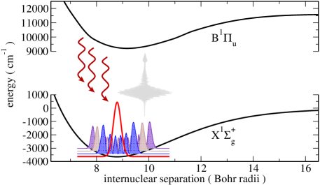
Figure 1: Potential energy curves of the Cs₂ electronic states employed for the vibrational cooling by optimized optical pumping and spontaneous emission. The vibrational ground state (red solid curve) is the target state of the optimization, vibrationally excited states (shown here $v=5,10,15$) make up the initial incoherent ensemble.

In the experiments of Refs. Viteau et al. (2008, 2009); Sofikitis et al. (2009, 2010); Lignier et al. (2011); Horchani et al. (2012); Manai et al. (2012, 2013), cooling the internal degrees of freedom by broadband optical pumping was preceded by standard laser cooling of atoms to temperatures of the order of 100$\,\mu$K and then photoassociating the atoms into weakly bound excited state molecules. Photoassociation Masnou-Seeuws and Pillet (2001); Jones et al. (2006) is followed by spontaneous emission, yielding molecules in the ground electronic state. Depending on the choice of excited state potential, a significant part of the molecules might end up in ground state levels with comparatively small vibrational quantum numbers Viteau et al. (2008); Lignier et al. (2011). These molecules can be laser cooled by broadband optical pumping as illustrated in Fig. 1: An incoherent ensemble of molecules in different vibrational levels of the electronic ground state is excited by a broadband laser pulse to an electronically excited state. The electronically excited molecules will decay by spontaneous emission back to the ground state. The branching ratio for the different ground state vibrational levels is determined by the Franck-Condon factors or, more precisely, transition matrix elements, between ground and excited state levels. Some decay will always lead to the ground vibrational level. Repeated broadband optical pumping then accumulates the molecules in the ground vibrational level Viteau et al. (2008).

The overall cooling rate is determined by the timescale of the dissipative step, i.e., the spontaneous emission lifetime Bartana et al. (1993, 1997, 2001). It cannot be modified by the coherent interaction of the molecules with the laser pulse. However, the pulses can be shaped such as to populate those excited state levels which preferentially decay into the target level. Here we show that this minimizes the number of required optical pumping cycles. Moreover, we demonstrate that optimal pulse shapes allow for cooling even in cases where the Franck-Condon map is preferential to heating rather than cooling. This is the case when the excited state levels show similar Einstein coefficients for many ground state vibrational levels. Rather than accumulating the molecules in a single target level, spontaneous emission then distributes the population incoherently over many levels, effectively heating the molecules up.

We employ optimal control theory to calculate the pulse shapes. Instead of treating the full dissipative dynamics of the excitation/spontaneous emission cycle, we take advantage of the timescale separation between the coherent interaction of the molecules with the laser pulse, on the order of 10 ps, and the spontaneous decay with excited state lifetimes of the order of 10 ns. Seeking a pulse that populates those excited state levels with the largest Einstein coefficients with the target ground state level allows us to treat the decay implicitly. We formulate two optimization functionals that are independent of the specific initial state. Thus we obtain an optimized pulse shape that remains unchanged over the complete cooling process consisting of many repeated excitation/spontaneous emission cycles. The two optimization functionals realize different cooling mechanisms: One is based on optical pumping from all thermally populated ground state levels symmetrically, whereas the other one forces the thermally populated ground state levels into an ’assembly line’. Only the first level in the line is transferred to the excited state while population from all other levels is reshuffled, one after the other into the first level, via Raman transitions. This suppresses heating actively and allows us to answer the question of what is the fundamental requirement of the molecular structure to allow for cooling.

Our paper is organized as follows. Section II introduces our model for the interaction of the molecules with the laser pulse and the spontaneous emission. We derive the optimization functionals for cooling in Sec. III and present our numerical results in Sec. IV, comparing vibrational laser cooling for Cs₂ and LiCs molecules. We conclude in Sec. V.

II Model

We consider Cs₂ and LiCs molecules in their electronic ground state after photoassociation and subsequent spontaneous emission. The excited state for optical pumping is chosen to be the $B^{1}\Pi_{u}$ state as in the experiment for Cs₂ molecules of Refs. Viteau et al. (2008, 2009); Sofikitis et al. (2009, 2010). This state is comparatively isolated such that population leakage to other electronic states due to e.g. spin-orbit interaction is minimal. The Hamiltonian describing the interaction of the molecules with shaped femtosecond laser pulses in the rotating-wave approximation reads

$$\boldsymbol{\mathsf{\hat{H}}}=\begin{pmatrix}\boldsymbol{\mathsf{\hat{T}}}+V_{X^{1}\Sigma^{+}}(\boldsymbol{\mathsf{\hat{R}}})&\frac{1}{2}\epsilon^{*}(t)\,\boldsymbol{\mathsf{\hat{\mu}}}\\ \frac{1}{2}\epsilon(t)\,\boldsymbol{\mathsf{\hat{\mu}}}&\boldsymbol{\mathsf{\hat{T}}}+V_{B^{1}\Pi}(\boldsymbol{\mathsf{\hat{R}}})-\omega_{L}\end{pmatrix}\,,$$ (1)

where $\boldsymbol{\mathsf{\hat{T}}}$ denotes the vibrational kinetic energy. $V_{g}=V_{X^{1}\Sigma^{+}}(\boldsymbol{\mathsf{\hat{R}}})$ and $V_{e}=V_{B^{1}\Pi}(\boldsymbol{\mathsf{\hat{R}}})$ are the potential energy curves as a function of interatomic separation, $\boldsymbol{\mathsf{\hat{R}}}$, of the electronic ground and excited state (note that for Cs₂ the $X$ state is of gerade symmetry and the $B$ state of ungerade symmetry). $\boldsymbol{\mathsf{\hat{\mu}}}$ is the transition dipole moment, approximated here to be independent of $\boldsymbol{\mathsf{\hat{R}}}$. The laser pulse is characterized by its carrier frequency, $\omega_{L}$, and complex shape, $\epsilon(t)=|\epsilon(t)|e^{i\phi(t)}$, with the time-dependent phase $\phi(t)$ referenced to the phase of the carrier frequency. The potential energy curves are found in Refs. Amiot and Dulieu (2002) and Staanum et al. (2007) for the electronic ground state and in Refs. Diemer et al. (1989) and Grochola et al. (2009) for the electronically excited state of Cs₂ and LiCs, respectively.

The decay of the excited state molecules back to the electronic ground state is described by the spontaneous emission rates,

$$\gamma_{v^{\prime}J^{\prime}}^{d}=\sum_{v^{\prime\prime}J^{\prime\prime}}A_{v^{\prime}J^{\prime},v^{\prime\prime}J^{\prime\prime}}\,.$$ (2)

The Einstein coefficients $A_{v^{\prime}J^{\prime},v^{\prime\prime}J^{\prime\prime}}$ are determined by the Franck-Condon factors,

$$A_{v^{\prime}J^{\prime},v^{\prime\prime}J^{\prime\prime}}=\frac{4\alpha^{3}}{3e^{4}\hbar^{2}}H_{J^{\prime}}(E_{v^{\prime}J^{\prime}}-E_{v^{\prime\prime}J^{\prime\prime}})^{3}\Big{|}\langle\varphi^{B}_{v^{\prime}J^{\prime}}|\boldsymbol{\mathsf{\hat{\mu}}}|\varphi^{X}_{v^{\prime\prime}J^{\prime\prime}}\rangle\Big{|}^{2}\,,$$ (3)

where $H_{J^{\prime}}$ is the Hönl-London factor equal to $(J^{\prime}+1)/(2J^{\prime}+1)$ for $J^{\prime}=J^{\prime\prime}-1$ and equal to $J^{\prime}/(2J^{\prime}+1)$ for $J^{\prime}=J^{\prime\prime}+1$, $\alpha$ denotes the fine structure constant and $e$ the electron charge. $|\varphi^{X}_{v^{\prime\prime}J^{\prime\prime}}\rangle$ and $|\varphi^{B}_{v^{\prime}J^{\prime}}\rangle$ are the rovibrational eigenstates of the $X^{1}\Sigma^{+}$ electronic ground state and the $B^{1}\Pi$ excited state, respectively. We will neglect rotations in the following since the Einstein coefficients are essentially determined by the Franck-Condon factors, $\langle\varphi^{B}_{v^{\prime}J^{\prime}}|\boldsymbol{\mathsf{\hat{\mu}}}|\varphi^{X}_{v^{\prime\prime}J^{\prime\prime}}\rangle\approx\langle\varphi^{B}_{v^{\prime}0}|\boldsymbol{\mathsf{\hat{\mu}}}|\varphi^{X}_{v^{\prime\prime}0}\rangle$.

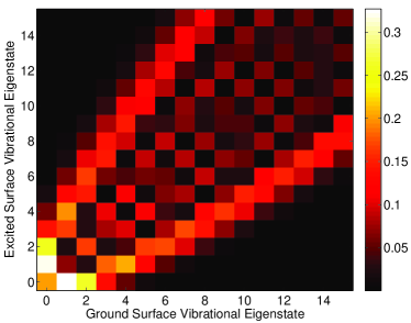
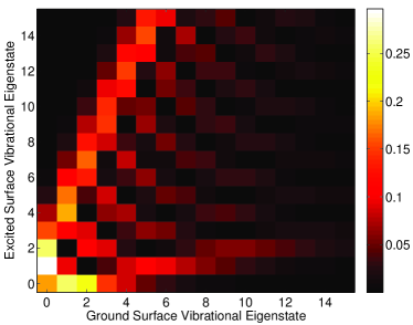
Figure 2: Franck-Condon map, $\langle\varphi^{B}_{v^{\prime}}|\boldsymbol{\mathsf{\hat{\mu}}}|\varphi^{X}_{v^{\prime\prime}}\rangle$, as a function of ground and excited state levels, $v^{\prime\prime}$ and $v^{\prime}$, respectively, for Cs₂ (left) and LiCs (right). Optical pumping at the right edge of the compact parabola for Cs₂ ensures cooling. This is in contrast to LiCs where absence of a compact boundary of the large transition matrix elements implies spontaneous emission towards levels with larger $v^{\prime\prime}$, i.e., heating.

Figure 2 displays the Franck-Condon map that governs the spontaneous emission for Cs₂ and LiCs. A compact parabola of large transition matrix elements is observed for Cs₂, cf. left-hand side of Fig. 2. Excitation at the right edge of this parabola can simply be ensured by removing part of the broadband spectrum Viteau et al. (2008). Spontaneous emission then will occur to levels with $v^{\prime\prime}\leq v_{initial}$, and repeated cycles of broadband excitation and spontaneous emission results in vibrational cooling Viteau et al. (2008). The situation changes completely for LiCs, cf. right-hand side of Fig. 2. There is no compact boundary separating large from small transition matrix elements, and a given excited state level has many non-zero transition matrix elements of similar magnitude. Spontaneous emission will thus spread the population, and even worse, will do so preferentially toward levels with $v^{\prime\prime}\geq v_{initial}$, leading to heating rather than cooling.

III Optimization functional for vibrational cooling of molecules

We will employ Krotov’s method Konnov and Krotov (1999); Sklarz and Tannor (2002); Palao and Kosloff (2003); Reich et al. (2012) to optimize vibrational cooling of molecules. The total optimization functional is then split into a final-time target $J_{T}$ and an intermediate-time cost $J_{t}$,

$$J=J_{T}+\int_{0}^{T}J_{t}\,dt\,,$$ (4)

and will be minimized. We choose the intermediate-time cost to minimize the change in pulse fluence Palao and Kosloff (2003),

$$J_{t}=\frac{\lambda}{S(t)}\left[\epsilon(t)-\epsilon_{ref}(t)\right]^{2}\,,$$ (5)

where $\lambda$ is a free parameter, $S(t)$ a shape function enforcing the pulses to be switched on and off smoothly and $\epsilon_{ref}(t)$ a reference field, taken to be the pulse from the previous iteration. The final time $T$ is also a free parameter.

We construct $J_{T}$ such as to avoid solution of the Liouville von Neumann equation for the density matrix during optimization. This is possible due to a separation of the timescales for spontaneous decay, of the order of 10 ns, and the coherent interaction of the molecules with laser light, of the order of 10 ps. Moreover, it allows for determining the laser field that is the best possible compromise, no matter what is the initial state. In other words, the same pulse can be used over and over again, accumulating molecules in the target state. We discuss two possible choices for the final-time functional.

III.1 Functional for exciting all vibrationally excited ground state levels symmetrically

The main idea of this functional is to excite all vibrationally excited ground state levels symmetrically into those excited state levels which preferentially decay toward the target state $|\varphi^{g}_{0}\rangle$ while minimizing potential heating. Symmetric excitation ensures that all ground state levels in the thermal ensemble are treated homogeneously. The initial state for each laser pulse is given by an unknown incoherent distribution over ground state vibrational levels, $|\psi_{i}(0)\rangle=|\varphi^{g}_{i}\rangle$, $i=1,\ldots,n_{max}$. Each of these levels is excited by the pulse and subject to the ensuing dynamics, giving rise to wavepackets $|\psi_{i}(t)\rangle$ which decay by spontaneous emission to ground state vibrational levels. The spontaneous decay of the excited state component of the $i$th wavepacket $|\psi_{i}(t)\rangle$ to the target level $|\varphi_{0}^{g}\rangle$ is determined by the temporally averaged overlap,

$$\sigma_{i}=\frac{1}{T_{e}}\int_{T}^{T+T_{e}}\left|\Braket{\psi_{i}(t)}{\boldsymbol{\mathsf{\hat{P}}}_{e}\,\boldsymbol{\hat{\mu}}}{\varphi_{0}^{g}}\right|^{2}dt\,,$$ (6)

where $T_{e}$ denotes the excited state lifetime and $\boldsymbol{\mathsf{\hat{P}}}_{e}$ is the projector onto the excited electronic state. Shifting the time axis by $-T$, inserting the completeness relation for vibrational levels on the excited state and denoting the Franck-Condon factors $\langle\varphi^{e}_{n}|\boldsymbol{\hat{\mu}}|\varphi^{g}_{m}\rangle$ by $\eta_{nm}$, Eq. (6) becomes

$$\sigma_{i}=\frac{1}{T_{e}}\int_{0}^{T_{e}}\sum_{n,m}e^{i(E^{e}_{n}-E^{e}_{m})t}\eta_{n0}\eta^{*}_{m0}\langle\psi_{i}(T)|\varphi^{e}_{n}\rangle\langle\varphi^{e}_{m}|\psi_{i}(T)\rangle dt\,,$$

where $E^{e}_{n}$ is the eigenenergy corresponding to $|\varphi^{e}_{n}\rangle$. The integral is readily evaluated, yielding

$$\sigma_{i}=\sum_{n\neq m}\frac{1}{iT_{e}(E^{e}_{n}-E^{e}_{m})}\left(e^{i(E^{e}_{n}-E^{e}_{m})t}-1\right)\eta_{n0}\eta^{*}_{m0}\langle\psi_{i}(T)|\varphi^{e}_{n}\rangle\langle\varphi^{e}_{m}|\psi_{i}(T)\rangle+\sum_{n}|\eta_{n0}|^{2}\left|\langle\psi_{i}(T)|\varphi^{e}_{n}\rangle\right|^{2}\,.$$

Due to the timescale separation, $1/(T_{e}(E^{e}_{n}-E^{e}_{m}))$ is at most of the order $10^{-4}$, and the temporally averaged overlap is well approximated by the second term alone,

$$\sigma_{i}=\sum_{n}|\eta_{n0}|^{2}\left|\langle\psi_{i}(T)|\varphi^{e}_{n}\rangle\right|^{2}\,.$$ (7)

The timescale separation also allows for neglecting the accidental creation of coherences in the ground state density matrix after each cooling cycle. While the initial ensemble most likely is a completely incoherent mixture, the state obtained on the ground electronic surface after one cooling cycle may contain coherences. Accidentally, this could lead to accumulation of molecules in an undesired dark state, i.e., a certain coherent superposition of vibrational eigenstates. However, the free evolution of the molecule introduces rapidly oscillating prefactors for each eigenstate. These oscillations are much more rapid than the time necessary for decay to the ground surface. Therefore, the system will be in a superposition of eigenstates with a fixed modulus but random phase before the next pulse arrives. If necessary, this can be strictly enforced by introducing a small, randomized waiting period between cycles. Since a dark state requires a fixed phase relation, accumulation in the dark state is effectively ruled out.

Ignoring coherences, the initial ensemble for each pulse is described only in terms of the vibrational populations, and maximizing the excitation of each vibrational level corresponds to minimizing

$$J_{yield}=1-\sum_{n=1}^{n_{max}}\sigma_{n}\,.$$ (8)

Symmetric excitation of all levels is ensured by balancing the yield with respect to an arbitrarily chosen level out of the initial ensemble, $1\leq n^{*}\leq n_{max}$,

$$J_{sym}=\sum_{n=1(n\neq n^{*})}^{n_{max}}\left(\sigma_{n}-\sigma_{n^{*}}\right)^{2}\,.$$ (9)

$J_{sym}$ is required because otherwise the yield could be maximized by very efficiently exciting only some levels in the initial ensemble. This would result in incomplete cooling. In addition to efficiently exciting all vibrationally excited ground state levels, the target state must be kept dark. This is achieved by enforcing the steady-state condition,

$$J_{ss}=1-\left|\langle\varphi^{g}_{0}|\boldsymbol{\mathsf{\hat{U}}}(T,0;\epsilon)|\varphi^{g}_{0}\rangle\right|^{2}\,.$$ (10)

A further complication arises from the fact that molecules could dissociate during the cooling process. This is a source of loss and needs to be strictly prevented. The most efficient way of enforcing this requirement is to avoid leakage out of the initial ensemble of ground state vibrational levels,

$$J_{leak}=\sum_{m^{\prime}=n_{max}+1}\sum_{m=0}^{n_{max}}\left|\langle\varphi^{g}_{m^{\prime}}|\boldsymbol{\mathsf{\hat{U}}}(T,0;\epsilon)|\varphi^{g}_{m}\rangle\right|^{2}+\sum_{m^{\prime}=n_{max}+1}\sum_{l}\sum_{m=0}^{n_{max}}|\eta_{lm^{\prime}}|^{2}\left|\langle\varphi^{e}_{l}|\boldsymbol{\mathsf{\hat{U}}}(T,0;\epsilon)|\varphi^{g}_{m}\rangle\right|^{2}\,.$$ (11)

The first term in Eq. (11) suppresses population transfer, via Raman transitions, from the initial ground state ensemble into higher excited ground state levels, whereas the second term suppresses population of excited state levels that have large Franck-Condon factors with ground state levels outside of the initial ensemble. $J_{leak}$ does not only counter dissociation of the molecules but also undesired heating.

The complete final-time functional is given by the multi-objective target of keeping the target state dark, efficiently exciting all other vibrational levels in the initial ensemble and avoiding leakage out of the initial ensemble,

$$J_{T}^{sym}=\lambda_{ss}J_{ss}+\lambda_{leak}J_{leak}+\lambda_{yield}J_{yield}+\lambda_{sym}J_{sym}\,,$$ (12)

where the $\lambda_{j}>0$ allow to weight the separate contributions differently. The functional (12) will yield optimized pulses that cool when used in repeated excitation/deexcitation cycles, unless the molecule under consideration has a Franck-Condon map that strongly favors heating rather than cooling such that simultaneously fulfilling all targets imposed by the functional becomes very difficult. This raises the question of what is the minimum requirement on the transition matrix elements to obtain cooling. It has led us to define a second optimization functional.

III.2 Functional for assembly-line cooling

The main idea of this functional is to optimize population transfer to the electronically excited state only for a single ground state level $n^{*}$. The excited state levels that are reached from $n^{*}$ need to have Franck-Condon factors that are favorable to cooling (in the extreme case, a single excited state level with favorable Franck-Condon factor is sufficient). The population of all other vibrationally excited ground state levels is simply reshuffled via Raman transitions, populating preferentially $n^{*}$. For example, if the cooling target is the ground state and we choose $n^{*}=1$, all higher levels are reshuffled into the next lower level, forming an ’assembly line’ which ends in $n=n^{*}$.

The corresponding functional contains the steady state and leakage terms just as Eq. (12). The excitation term now targets only $n^{*}$, taken to be $n^{*}=1$,

$$\tilde{J}_{yield}=1-\sigma_{1}\,,$$ (13)

and population reshuffling towards lower vibrational levels is enforced by the assembly-line term,

$$J_{ass}=1-\frac{1}{n_{max}-1}\sum_{n=2}^{n_{max}}\left|\langle\varphi^{g}_{n-1}|\boldsymbol{\mathsf{\hat{U}}}(T,0;\epsilon)|\varphi^{g}_{n}\rangle\right|^{2}\,.$$ (14)

Similarly to Eq. (12), the complete final-time functional for assembly line cooling is given by summing all contributions,

$$J^{ass}_{T}=\lambda_{ss}J_{ss}+\lambda_{leak}J_{leak}+\lambda_{yield}\tilde{J}_{yield}+\lambda_{ass}J_{ass}$$ (15)

with weights $\lambda_{j}>0$. In Eq. (12), heating is countered only via the leakage term, whereas Eq. (15) avoids it actively.

III.3 Krotov’s method for vibrational cooling

The optimization functionals, Eq. (12) and Eq. (15), represent the starting point for deriving the coupled control equations that must be solved iteratively to obtain the optimized pulse. Following Krotov’s method Reich et al. (2012), we obtain a set of three equations with prescribed discretization for each iteration step $i$:

• Forward propagation of each state in the initial thermal ensemble according to

  $$i\hbar\frac{\partial}{\partial t}|\psi^{(i+1)}_{n}(t)\rangle=\boldsymbol{\mathsf{\hat{H}}}[\epsilon^{(i+1)}]|\psi^{(i+1)}_{n}(t)\rangle\,,\quad|\psi^{(i+1)}_{n}(t=0)\rangle=|\varphi^{g}_{n}\rangle\,,\quad n=1,\ldots,n_{max}\,,$$ (16)

  with $\boldsymbol{\mathsf{\hat{H}}}$ given by Eq. (1).

• Backward propagation of the adjoint states,

  $$i\hbar\frac{\partial}{\partial t}|\chi^{(i)}_{n}(t)\rangle=\boldsymbol{\mathsf{\hat{H}}}[\epsilon^{(i)}]|\chi^{(i)}_{n}(t)\rangle\,,\quad|\chi^{(i)}_{n}(t=T)\rangle=\nabla_{\langle\psi_{n}|}J^{sym/ass}_{T}\big{|}_{\{|\psi^{(i)}(T)\rangle\}}\quad n=1,\ldots,n_{max}\,,$$ (17)

  with the ’initial’ condition at time $t=T$ given by the derivatives of the final-time functional, Eq. (12) or Eq. (15), with respect to $\langle\psi_{n}|$, evaluated using the final-time forward propagated states, $|\psi^{(i)}_{n}(T)\rangle$.

• Update of the control by

  $$\epsilon^{(i+1)}(t)=\epsilon^{(i)}(t)+\frac{S(t)}{\lambda}\mathfrak{Im}\left\{\sum_{n=1}^{n_{max}}\langle\chi_{n}^{(i)}(t)|\boldsymbol{\hat{\mu}}|\psi_{n}^{(i+1)}(t)\rangle+\frac{1}{2}\sigma(t)\sum_{n=1}^{n_{max}}\langle\psi_{n}^{(i+1)}(t)-\psi_{n}^{(i)}(t)|\boldsymbol{\hat{\mu}}|\psi_{n}^{(i+1)}(t)\rangle\right\}$$ (18)

  with $|\psi_{n}^{(i+1)}(t)\rangle$, $|\psi_{n}^{(i)}(t)\rangle$ and $|\chi_{n}^{(i)}(t)\rangle$ solutions of Eqs. (16) and (17), respectively. $J_{T}^{sym}$ is a polynomial of fourth order in the states, whereas $J_{T}^{ass}$ is quadratic in the states. This means that $J_{T}^{sym}$ requires the non-linear version of Krotov’s method, and $\sigma(t)$ is given by $\sigma(t)=-(2A+\epsilon_{A})$ Reich et al. (2012). For $J_{T}^{ass}$, the linear version is sufficient, i.e., $\sigma(t)=0$. $A$ can be estimated analytically by evaluating a supremum over the second order derivatives of $J_{T}^{sym}$, and $\epsilon_{A}$ is a non-negative number. The analytical estimate of $A$ usually is much larger than the actual value of $A$ required to ensure monotonicity of the algorithm. Since a large value of $A$ slows down convergence, it is much better to approximate $A$ numerically, using Eq. (25) of Ref. Reich et al. (2012).

It turned out, however, that the non-convexity of $J^{sym}_{T}$ is small in practice, and both the linear and the non-linear version of Krotov’s method behave very similarly. This can be rationalized by the fact that only one term in $J_{T}^{sym}$, $J_{sym}$, is non-convex and its impact on the convergence is small compared to that of the other terms in $J_{T}^{sym}$. The results presented below were all obtained for $\sigma(t)=0$ in Eq. (18).

Instead of the square modulus in the overlaps of Eqs. (7), (10), (11) and (14), it is also possible to use the real part of the overlap Palao and Kosloff (2003). This sets a global phase which is not neccessary but shows a better initial convergence for bad guess pulses. The latter is due to the specific form of the ’initial’ costates, $|\chi_{n}^{(i)}(T)\rangle$, which remain constant for real part functionals while depending linearly on the final-time forward propagated states, $|\psi_{n}^{(i)}(T)\rangle$, for the square modulus functional. Hence real part functionals cannot take values close to zero leading to very small gradients as is the case for square modulus functionals. This is important in particular for the assembly-line term, for which formulating a good guess pulse is difficult, and our results presented below were obtained with the real part instead of the square modulus in Eq. (14).

IV Optimization results

We choose our guess pulses such as to avoid small gradients at the beginning of the optimization. In all examples, they are taken to be Gaussian transform-limited pulses of moderate intensity with central frequency and spectral width chosen to excite a number of transitions that are relevant for the cooling process. The latter are easily read off the Franck-Condon matrices in Fig. 2. The choice of the $\lambda_{j}$ is determined by the relative importance of the individual terms in the optimization functionals. A large value for the steady-state and leakage terms are impedient since a low value of these functionals will prevent a high repeatability of the excitation/deexcitation steps, effectively reducing the attainable yield. In contrast, a slightly lower yield for an individualy step can easily be amended by few additional cycles. Consequently, as a rule of thumb, $\lambda_{ss}$ and $\lambda_{leak}$ should be chosen larger than $\lambda_{yield}$ and $\lambda_{sym}$ or $\lambda_{ass}$, respectively. This is more important for the symmetrised cooling since in the assembly line case the leakage is much easier to prevent by virtue of the mechanism. Hence it proved in our calculation sufficient to choose all $\lambda$ equal to one for the assembly line functional while it proved useful to choose $\lambda_{leak}=\lambda_{sym}=1$, $\lambda_{ss}=2$ and $\lambda_{yield}=0.4$ for the symmetrised functional.

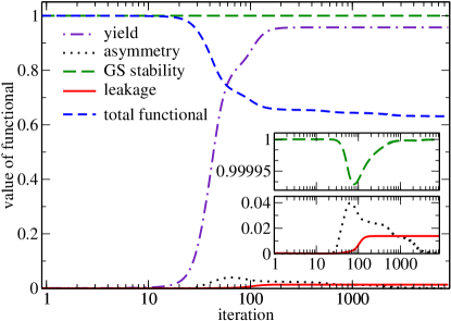
Figure 3: Optimizing the vibrational cooling of Cs₂ molecules using symmetrized excitation: Value of the total functional, Eq. (12), and its components vs iterations of the optimization algorithm ($n_{max}=10$).

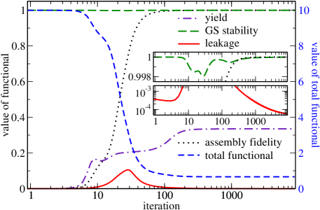
Figure 4: Optimizing the vibrational cooling of Cs₂ molecules using assembly-line cooling: Value of the total functional, Eq. (15), and its components vs iterations of the optimization algorithm ($n_{max}=10$).

We first study vibrational cooling of Cs₂ molecules, taking $n_{max}=10$. Due to the favorable Franck-Condon map, optimization is not required in this case but helps to reduce the number of cooling cycles. The behavior of the single contributions to the optimization functional as well as its total value are plotted in Fig. 3 for $J_{T}^{sym}$ and in Fig. 4 for $J_{T}^{ass}$. In both cases, monotonous convergence is observed for the total functional as expected, cf. blue dashed lines in Figs. 3 and 4. The dark-state condition for the target state is perfectly obeyed for symmetrized excitation throughout the optimization (green long-dashed line in the inset of Fig. 3) but presents a slightly more difficult constraint to fulfill for assembly-line cooling (green long-dashed line in the inset of Fig. 4, note that the stability of the ground state is given by $1-J_{ss}$). A final value of $1-J_{ss}=9\cdot 10^{-6}$ ensures also for assembly-line cooling accumulation in the target state for 10000 cooling cycles. This is much more than required as we show below. For optimization using $J_{T}^{sym}$, the excitation yield, given by $1-J_{yield}$, measures excitation of all levels in the initial ensemble, and reaches a value above 0.9, cf. purple dot-dashed line in Fig. 3. This together with the fact that the final value of $J_{sym}$ (black dotted line in Fig. 3) is $10^{-6}$ implies that a pulse that excites all levels in the initial ensemble with similar efficiency can indeed be found. For optimization using $J_{T}^{ass}$, the excitation yield, $1-\tilde{J}_{yield}$, takes a smaller final value (purple dot-dashed line in Fig. 4). This reflects the fact that $1-\tilde{J}_{yield}$ measures only excitation out of $v^{\prime\prime}=1$ and its maximum is given by 0.335, whereas the population reshuffling of the other levels is captured by $1-J_{ass}$ (black dotted line in Fig. 4). The latter takes a final value close to one, suggesting that the pulse reshuffles all higher excited ground state levels in the desired way. This indicates efficient excitation at the end of the assembly line as desired. Thus both optimization functionals, Eq. (12) and Eq. (15), yield pulses which effectively excite all higher vibrational levels while keeping the target state dark. A striking difference between optimization with $J_{T}^{sym}$ and $J_{T}^{ass}$ is found only in the ability of the optimized pulses to suppress leakage out of the initial ensemble (red solid lines in Fig. 3 and 4). While $J_{leak}$ takes a final value of about 0.014 for symmetrized excitation, it can be made smaller than $10^{-4}$ for assembly line cooling. In the latter case, $J_{leak}$ could be further decreased by continued optimization, cf. the slope of the red line in Fig. 4. This is in contrast to Fig. 3 where $J_{leak}$ remains essentially unchanged after about 200 iterations, suggesting that a hard limit has been reached. Leakage from the cooling subspace thus starts to pose a problem for symmetrized excitation when a few hundred cooling cycles are required. The different performance of the two optimization functionals is not surprising since $J_{T}^{ass}$ is constructed to actively suppress leakage from the initial ensemble (and the ensuing vibrational heating) by allowing spontaneous emission only from the most favorable instead of all accessible levels. The extent to which leakage can be suppressed when employing $J_{T}^{ass}$ is nonetheless very gratifying.

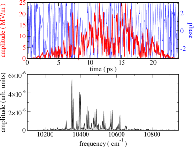
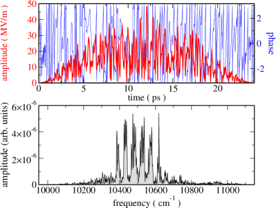
Figure 5: Optimized pulses (top) and their spectra (bottom) for the vibrational cooling of Cs₂ molecules using symmetrized excitation (left) and assembly-line cooling (right).

The optimized pulses and their spectra for vibrational cooling of Cs₂ are shown in Fig. 5, comparing symmetrized excitation (left-hand side) and assembly-line cooling (right-hand side). The spectral width of the optimized pulses covers about 500 cm^-1 corresponding to transform-limited pulses of 30 fs. This is well within the standard capabilities of current femtosecond technology. A similar conclusion can be made with respect to the integrated pulse energies: We find $1\,\mu$J for the pulse obtained with $J_{T}^{sym}$ in the left-hand side of Fig. 5 and $4\,\mu$J for that obtained with $J_{T}^{ass}$ in the right-hand side of Fig. 5.

We now turn to the example of LiCs molecules for which the Franck-Condon map is not favorable to cooling. Broadband optical pumping with unshaped pulses will thus lead to heating rather than cooling, cf. Fig. 2. We demonstrate in the following that shaping the pulses does, however, yield vibrational cooling. Note that by employing the $B^{1}\Pi$-state, we have chosen the most favorable out of all potential energy curves correlating to the lowest excited state asymptote (Li 2s + Cs 6p). For example, the $A^{1}\Sigma^{+}$ state is expected to be even less suited for cooling. While the $A^{1}\Sigma^{+}$-state potential is more deeply bound and could thus be somewhat better in terms of the Franck-Condon map, it is strongly perturbed by the spin-orbit interaction. The resulting coupling to triplet states implies a loss from the cooling cycle that, due to the timescale separation of excitation and spontaneous emission, cannot be prevented by shaping the pulse.

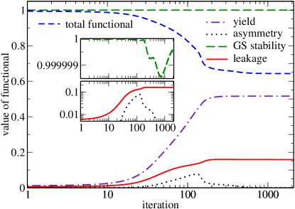
Figure 6: Optimizing the vibrational cooling of LiCs molecules using symmetrized excitation: Value of the total functional, Eq. (12), and its components vs iterations of the optimization algorithm ($n_{max}=5$).

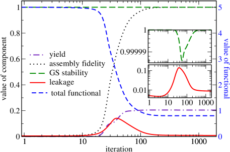
Figure 7: Optimizing the vibrational cooling of LiCs molecules using assembly-line cooling: Value of the total functional, Eq. (15), and its components vs iterations of the optimization algorithm ($n_{max}=5$).

Since the $B^{1}\Pi$-state of LiCs is comparatively shallow Grochola et al. (2009), leakage out of the initial ensemble and dissociation of the molecules is a more severe problem than for Cs₂. We therefore first discuss $n_{max}=5$ and show later that assembly-line cooling allows also for larger $n_{max}$. The behavior of the optimization functionals and their single contributions is displayed in Fig. 6 for $J_{T}^{sym}$ and in Fig. 7 for $J_{T}^{ass}$. The overall behavior of the functionals and their components is very similar to that observed for Cs₂ in Figs. 3 and 4. In particular, both algorithms converge monotonically (dashed blue lines in Figs. 6 and 7), the dark-state condition can be very well fulfilled (green long dashed lines), and the excitation is efficient (purple dot-dashed and black dotted lines). The behavior with respect to leakage changes, however, dramatically when going from Cs$2$ to LiCs (red lines in Figs. 6 and 7): $J_{leak}$ takes final values of 0.16 for symmetrized excitation and 0.009 for assembly-line cooling. This reflects the Franck-Condon map being so much more favorable to heating rather than cooling, cf. Fig. 2 (right), that even with shaped pulses it is difficult to ensure cooling. In particular, the result for symmetrized excitation is insufficient since $J_{leak}=0.16$ implies that losses from the cooling cycle will occur already after few excitation/deexcitation steps. For $n_{max}=5$, $J_{leak}$ reaches a plateau for symmetrized excitation and assembly-line cooling alike. This is easily rationalized by inspection of the Franck-Condon map in Fig. 2 (right). In particular, the excited state levels which are reached from $v^{\prime\prime}=5$, such as $v^{\prime}=2$, show a large leakage toward higher ground state vibrational levels. We have therefore also investigated $n_{max}=10$ for assembly-line cooling. Most of the levels into which e.g. $v^{\prime}=2$ decays and which represent leakage for $n_{max}=5$ are then part of the ensemble. Indeed, we find $J_{leak}=0.002$ after 1000 iterations for $n_{max}=10$ (data not shown). Moreover, $J_{leak}$ continues to decrease after 1000 iterations, albeit not as steeply as in Fig. 4 for Cs₂, allowing to push the value of $J_{leak}$ below $10^{-3}$.

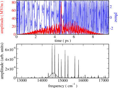
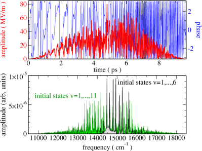
Figure 8: Optimized pulses (top) and their spectra (bottom) for the vibrational cooling of LiCs molecules using symmetrized excitation (left, $n_{max}=5$) and assembly-line cooling (right, $n_{max}=5$ in the top panel, $n_{max}=5$ and 10 in the bottom panel).

Figure 8 shows the optimized pulses (top) and their spectra (bottom) for LiCs with $n_{max}=5$ and symmetrized excitation (left) and assembly-line cooling (right). The bottom left panel of Fig. 8 displays furthermore the spectrum of the optimized assembly-line pulse obtained for $n_{max}=10$. The spectral width obtained for $n_{max}=5$ covers less than 3000 cm^-1, corresponding to the bandwidth of a transform-limited pulse of a few femtoseconds. The integrated pulse energy amounts to $3.4\,\mu$J. For $n_{max}=10$, significantly more transitions need to be driven, cf. Fig. 2. It is thus not surprising that both the spectral width of the optimized pulse and its integrated energy are larger than for $n_{max}=5$. The latter amounts to $16\,\mu$J. Such a pulse is more difficult to realize experimentally than those found for Cs₂. The spectral width could be reduced by employing spectral constraints Reich et al. (2013); Palao et al. (2013). The main point of our current investigation is, however, to demonstrate that optimized pulses lead to vibrational cooling even for molecules with unfavorable Franck-Condon map. This is evident from Fig. 7 and further substantiated by simulating the cooling process using the optimized pulses.

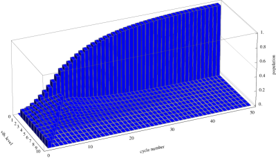
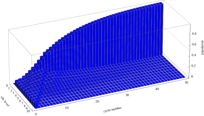
Figure 9: Demonstration of assembly-line cooling for Cs₂ (left) and LiCs (right) molecules: Population of ground state vibrational levels vs number of ecxitation/spontaneous emission cycles. The initial distribution is assumed to be an equipartition in the ground state vibrational levels $v^{\prime\prime}=1,\ldots,v^{\prime\prime}=10$.

	cooling	no. of cycles for 90%	max. target state yield	no. of cycles for max. yield
Cs2 ($n_{max}=10$)	$J_{T}^{sym}$	23	0.992	125
Cs2 ($n_{max}=10$)	$J_{T}^{ass}$	26	0.9993	100
LiCs ($n_{max}=5$)	$J_{T}^{sym}$	not achieved	0.80	97
LiCs ($n_{max}=5$)	$J_{T}^{ass}$	26	0.96	137
LiCs ($n_{max}=10$)	$J_{T}^{ass}$	30	0.99	84

Table 1: Accumulation of molecules in the target $v^{\prime\prime}=0$ level.

To this end, we assume the initial incoherent ensemble to be given by equal population in levels $v^{\prime\prime}=1,\ldots,10$ of the electronic ground state for both Cs₂ and LiCs. We calculate the wavepacket dynamics under the optimized pulse, and determine the ensemble that represents the initial state for the next pulse, identical to the previous one, by redistributing the population according to the Einstein coefficients, Eq. (3). The depletion of the excited vibrational levels and accumulation of population in $v^{\prime\prime}=0$ is imposingly demonstrated in Fig. 9 and Table 1. A ground state population of 90% is obtained after just a few tens of excitation/spontaneous emission cycles for both Cs₂ and LiCs. This is in contrast to spectrally cut pulses without any further shaping which require several thousand cycles for Cs₂ and would fail altogether for LiCs. Moreover, a high degree of purity, $\mathcal{P}>0.98$, is obtained for our optimized pulses with only of the order of 100 excitation/spontaneous emission cycles for both molecules.

V Summary and conclusions

We have adapted optimal control theory for cooling internal degrees of freedom to account for the timescale separation between coherent excitation and spontaneous emission. Our approach is based on a basis set expansion of the initial density matrix into vibrational eigenstates. This has allowed us to carry optimization of vibrational cooling from toy models Bartana et al. (1993, 1997, 2001) to a first principles description of alkali dimer molecules that are currently studied in cooling experiments Viteau et al. (2008, 2009); Sofikitis et al. (2009, 2010); Lignier et al. (2011); Horchani et al. (2012); Wakim et al. (2012). Compared to the earlier theoretical predictions where a single long pulse implemented the complete cooling process Bartana et al. (1993, 1997, 2001), our approach allows for finding femtosecond pulses that can be repeatedly applied, just as is done in the experiments. Shaping the pulses using optimal control allows to significantly reduce the number of excitation/spontaneous emission cycles and reach a high purity of the ground state molecules. More importantly, it also enables vibrational cooling for molecules where the Franck-Condon map favors heating rather than cooling.

The derivation of our optimization functionals was based on two different intuitions. First, simultaneous, symmetric excitation of all ground state levels in the thermal ensemble to the excited state was expected to yield most efficient cooling. It turned out, however, that this approach has only a limited capability of suppressing leakage out of the initial ensemble to higher lying levels. In particular for molecules with unfavorable Franck-Condon map, this algorithm cannot avoid vibrational heating and, in extreme cases, dissociation. We have therefore devised an optimization functional corresponding to ’assembly-line’ cooling where only one ground state level is transferred to the excited state while the population of all other vibrationally excited ground state levels is reshuffled via Raman transitions. This approach yields pulses that enforce vibrational cooling even for molecules with transition matrix elements favoring heating rather than cooling. The spectral widths and integrated energies of our optimized pulses are well within the capabilities of current femtosecond technology. We have demonstrated successful implementation of cooling by calculating the population redistribution over a number of excitation/spontaneous emission steps, proving accumulation of ground state molecules.

Our study demonstrates the power of optimal control theory for reaching a control target that might not be accessible by simple, analytical pulse shapes. However, it also illustrates that optimal control theory is not a black-box tool but requires physical insight, in particular when constructing the optimization functional. This is crucial when one wants to address fundamental limits for control. In our case, this corresponds to the question of the minimum requirement on the molecular structure that is necessary to allow for cooling. The answer to this question determines the controllability of the problem, irrespective of the actual experimental resources such as pulse bandwidth or power. We find that all that is required is a single excited state level with moderate spontaneous decay probability to the target state and a limited number of significant transition matrix elements for the other ground state vibrational levels.

Laser cooling makes use of the simplest quantum reservoir, the vacuum of electric field modes, and has led to the concept of quantum reservoir engineering Poyatos et al. (1996). Analogously, our optimization approach for laser cooling can be generalized to quantum reservoir engineering. Since the creation of coherences cannot be neglected in the general case, this requires a basis set expansion in Liouville space rather than Hilbert space. Such a generalization of our optimal control approach to quantum reservoir engineering is currently in progress.