Compressive Sampling for Remote Control Systems

Abstract.

In remote control, efficient compression or representation of control signals is essential to send them through rate-limited channels. For this purpose, we propose an approach of sparse control signal representation using the compressive sampling technique. The problem of obtaining sparse representation is formulated by cardinality-constrained $\ell^{2}$ optimization of the control performance, which is reducible to $\ell^{1}\text{-}\ell^{2}$ optimization. The low rate random sampling employed in the proposed method based on the compressive sampling, in addition to the fact that the $\ell^{1}\text{-}\ell^{2}$ optimization can be effectively solved by a fast iteration method, enables us to generate the sparse control signal with reduced computational complexity, which is preferable in remote control systems where computation delays seriously degrade the performance. We give a theoretical result for control performance analysis based on the notion of restricted isometry property (RIP). An example is shown to illustrate the effectiveness of the proposed approach via numerical experiments.

1. Introduction

Remote control systems are those in which the controlled objects are located away from the control signal generators. They are widely used at the present day, from video games [1] to spacecraft [2], see [3] for other examples. In remote control systems, control signals are to be transmitted through rate-limited channels such as wireless channels [4] or the Internet [5]. In such systems, efficient signal compression or representation is essential to send control signals through communication channels. For this purpose, we propose an approach of sparse control signal representation using the compressive sampling technique [6, 7, 8] for remote control systems.

Compressive sampling, also known as compressed sensing, is a technique for acquiring and reconstructing signals in the sparse-land [9]. Signal acquisition and reconstruction is one of the fundamental issues in signal processing. In many applications, signals are analog (or continuous-time) before they are acquired and converted to digital (or discrete-time) signals. The problem is how to acquire and convert analog signals to digital ones without much information distortion, such as aliasing. A well-known and widely-used solution to this problem is Shannon’s sampling theorem [10, 11]. This theorem gives an acquisition and reconstruction method for perfect reconstruction; if the sampling rate is faster than twice the Nyquist rate, the maximum frequency contained in the original analog signal, then the original signal can be perfectly reconstructed via sinc series. On the other hand, in the sparse-land, signals are sparse or compressible under a certain signal representation (e.g., Fourier or wavelet). This sparsity assumption on signals is known to be valid for many real signals, e.g., see examples in [12]. Compressive sampling is based on this fact, by which one can reconstruct the original signal with very high fidelity from far fewer samples than what the conventional sampling theorem requires. Hence signal acquisition and compression can be performed in much more efficient manner, than the conventional scheme such as the image compression JPEG [13], where one acquires the full signal, then transforms it into the frequency domain, and finally discards most of them to obtain a compressed signal.

The purpose of this paper is to propose to use compressive sampling for remote control systems. Our contributions in this paper are as follows:

• We propose a new feed-forward-based remote control system with compressive sampling.

• The proposed system can efficiently compress the control signals with sparse representation.

• The design problem is formulated by $\ell^{1}\text{-}\ell^{2}$ optimization which can be efficiently solved.

The theory of compressive sampling has been applied to not only signal processing but also statistics [14], information theory [15], machine learning [16], and so on. For theory and application of compressive sampling, see books [17, 18, 12]. However, to the best of our knowledge, so far only a few studies have applied compressive sampling to control: [19] proposes to use compressive sensing in feedback control systems for perfect state reconstruction and [20] proposes sparse representation of transmitted control packets for feedback control. For remote control systems, [21] also proposes to use $\ell^{1}\text{-}\ell^{2}$ optimization as in this paper, but the compressive sampling technique (Fourier expansion and random sampling) is not used. As we mentioned above, it is desirable that signals in remote control systems are effectively acquired and compactly compressed. Therefore, we propose to adopt compressive sampling technique to remote control systems.

Compressive sampling in this paper can be considered as a kind of lossy compression. In many lossy data compression problems, the objective is to find efficient approximate representations of the original data [22], and the distortion is measured by the signal reconstruction error. On the other hand, in this paper, we consider a different aspect of the distortion, that is, we measure the efficiency of the lossy compression with control performance. In other words, our method aims at optimizing the control performance, e.g., minimizing the tracking error, while usual compressive sampling minimizes the $\ell^{2}$ norm of the reconstruction error, with a sparsity constraint. This is a natural notion in control; we do not care about how small the compression error of the control signal is but how good the control performance is. Thus we call the proposed approach control-oriented compressive sampling.

In remote control systems, control delays due to heavy computation seriously degrade the performance. In compressive sampling, signal acquisition is realized by a random non-uniform sampler [7] or a random demodulator [23], which takes almost no computational time. In contrast, obtaining sparse representation of a signal is achieved by solving $\ell^{1}\text{-}\ell^{2}$ optimization [24], also known as LASSO [25] or basis pursuit de-noising [26]. The solution to the $\ell^{1}\text{-}\ell^{2}$ optimization cannot be represented in an analytical form as in $\ell^{2}$ optimization, and hence we resort to iteration method to achieve the optimal solution. There have been recently a number of researches on this type of optimization, and there are several efficient algorithms for the solution [27, 28, 24]. Moreover, the low rate random sampling leads to reduced computational complexity of optimization. That is, we can use such computationally efficient algorithms with the low rate sampling in remote control to reduce control delays.

The paper is organized as follows: In Section 2, we define our control problem. In Section 3, we formulate and solve the problem via conventional sampling theorem. In Section 4, we propose a new control method based on compressive sampling. Section 5 gives a theoretical result for performance analysis of the proposed control. We show a numerical example in Section 6 to illustrate the effectiveness of the proposed method. Finally, we make a conclusion in Section 7.

Notation

In this paper, we use the following notation. ${\mathbb{Z}}$, ${\mathbb{R}}$ and ${\mathbb{C}}$ denote the sets of integral, real and complex numbers, respectively. ${\mathbb{R}}^{n}$ and ${\mathbb{R}}^{m\times n}$ (${\mathbb{C}}^{n}$ and ${\mathbb{C}}^{m\times n}$) denote the sets of $n$-dimensional real (complex) vectors and $m\times n$ matrices, respectively. We use ${\mathrm{j}}$ for the imaginary unit in ${\mathbb{C}}$. For a complex number $z\in{\mathbb{C}}$, $\bar{z}$ and ${\mathrm{Re}}~{}z$ represent the conjugate and the real part of $z$, respectively. For a matrix (a vector) $M$, $M^{\top}$ and $M^{\ast}$ represent the transpose and the Hermitian conjugate of $M$, respectively. For a vector ${\boldsymbol{v}}=[v_{1},\ldots,v_{n}]^{\top}\in{\mathbb{C}}^{n}$, we define $\ell^{0}$ “norm” $\|{\boldsymbol{v}}\|_{0}$ of ${\boldsymbol{v}}$ as the number of the nonzero elements in ${\boldsymbol{v}}$, and also define $\ell^{1}$ , $\ell^{2}$, and $\ell^{\infty}$ norms as

$$\|{\boldsymbol{v}}\|_{1}:=\sum_{i=1}^{n}|v_{i}|,~{}~{}\|{\boldsymbol{v}}\|_{2}:=\sqrt{{\boldsymbol{v}}^{\ast}{\boldsymbol{v}}},~{}~{}\|{\boldsymbol{v}}\|_{\infty}:=\max_{i=1,\ldots,n}|v_{i}|,$$

respectively. For a finite set $I=\{I_{1},\ldots,I_{K}\}\subset{\mathbb{Z}}$, we define $|I|:=K$. We denote by $L^{2}[0,T]$ the Lebesgue space consisting of all square integrable functions on $[0,T]\subset{\mathbb{R}}$, endowed with the inner product

$$\langle x,y\rangle:=\int_{0}^{T}x(t)\overline{y(t)}~{}{\mathrm{d}}t,\quad x,y\in L^{2}[0,T],$$

and the $L^{2}$ norm $\|x\|:=\sqrt{\langle x,x\rangle}$.

2. Control Problem

In this paper, we consider a control problem of a linear system $P$ on a finite time interval (or horizon) $[0,T]$, $T>0$, given by

$$P:\left\{\begin{split}\dot{{\boldsymbol{x}}}(t)&=A{\boldsymbol{x}}(t)+{\boldsymbol{b}}u(t),\\ y(t)&={\boldsymbol{c}}^{\top}{\boldsymbol{x}}(t),\quad{\boldsymbol{x}}(0)={\boldsymbol{x}}_{0}\in{\mathbb{R}}^{\nu},\quad t\in[0,T],\end{split}\right.$$ (1)

where $A\in{\mathbb{R}}^{\nu\times\nu}$, ${\boldsymbol{b}},{\boldsymbol{c}}\in{\mathbb{R}}^{\nu\times 1}$. In this equation, ${\boldsymbol{x}}(t)\in{\mathbb{R}}^{\nu}$ is the state, $u(t)\in{\mathbb{R}}$ is the input, and $y(t)\in{\mathbb{R}}$ is the output of the system $P$. The initial state ${\boldsymbol{x}}_{0}\in{\mathbb{R}}^{\nu}$ is assumed to be given. We also assume that the system is stable, that is, the eigenvalues of $A$ are in ${\mathbb{C}}_{-}=\{\lambda\in{\mathbb{C}}:{\mathrm{Re}}~{}\lambda<0\}$. Then the system $P$ can be considered as a bounded operator in $L^{2}[0,T]$ for any $T>0$. We use the notation $y=Pu$ for representing the input/output relation of the linear system $P$.

Figure 1. Linear system $P$ to be controlled. The control signal $u$ is transmitted through a communication channel. The initial state ${\boldsymbol{x}}_{0}$ is assumed to be measured.

Fig. 1 shows the block diagram of the system $P$ with the input $u$, the output $y=Pu$, and the initial state ${\boldsymbol{x}}_{0}$.

In order to show the significance of the proposed approach, we consider tracking problem in this paper as an example of the control problem. In the tracking problem, the controller attempts to reduce the tracking error between a given reference $r$ and the output $y=Pu$ over $[0,T]$. In other words, we design a control signal $\{u(t)\}_{t\in[0,T]}$ for a reference signal $\{r(t)\}_{t\in[0,T]}$ such that $r\approx Pu$ over $[0,T]$. More precisely, the control object is described as follows: Find a control signal $\{u(t)\}_{t\in[0,T]}$ such that

1. the tracking error $E(u):=\lVert Pu-r\rVert^{2}$ is small,

2. the “size” ${\bf{\Omega}}(u)$ of the control signal $u$ is not too large,

3. and the maximum frequency contained in $u$ is bounded by a fixed frequency.

The first objective is for tracking performance; if $E(u)$ is smaller, the performance is said to be better. Theoretically, $E(u)$ can be made arbitrarily small if the size ${\bf{\Omega}}(u)$ is not restricted.

Example 1.

Let $\hat{P}(s)$ denote the Laplace transform of the impulse response of the linear system $P$. Suppose $\hat{P}(s)$ is given by

$$\hat{P}(s)=\frac{s-\alpha}{s+\alpha},$$

where $\alpha>0$, and the reference $r$ is given in the Laplace transform by $\hat{r}(s)=1/s$. Then if we choose $u$ with its Laplace transform

$$\hat{u}(s)=\hat{P}(s)^{-1}\hat{r}(s)=\frac{s+\alpha}{s(s-\alpha)},$$

then the performance in terms of the tracking error will be perfect, that is, $E(u)=0$ over $[0,T]$. However, the inverse Laplace transform of $\hat{u}(s)$ is given by $u(t)=2\exp(\alpha t)-1$, $t\in[0,\infty)$, and hence $u(t)$ has the property $\lim_{t\rightarrow\infty}u(t)=\infty$ since $\alpha>0$. That is, if $T$ becomes large, then $|u(T)|$ increases exponentially. $\Box$

This example is not a special case; we can generally say that a small tracking error leads to a large control signal if $\hat{P}(s)$ has an unstable zero, that is, there exists $z\in{\mathbb{C}}_{+}=\{z\in{\mathbb{C}}:{\mathrm{Re}}~{}z\geq 0\}$ such that $\hat{P}(z)=0$. For example, suppose that the size of $u$ is measured by ${\bf{\Omega}}(u)=\lVert u\rVert^{2}$, the energy of the control signal $u$. As mentioned above, a smaller tracking error $E(u)$ leads to a larger energy ${\bf{\Omega}}(u)=\lVert u\rVert^{2}$. It follows that we have to transmit the information of a signal with a very large energy through a communication channel. In many cases, a larger energy results in a larger amplitude of a signal, and hence the variance becomes larger if the mean of $u(t)$ is $0$. This implies that the entropy of the signal increases and so does the amount of information. Moreover, large ${\bf{\Omega}}(u)$ leads to high sensitivity to noise in measurement of the initial value ${\boldsymbol{x}}_{0}$ or uncertainty in the model parameters $A$, ${\boldsymbol{b}}$, and ${\boldsymbol{c}}$. We therefore add a constraint on ${\bf{\Omega}}(u)$ as the second control objective. The size ${\bf{\Omega}}(u)$ is not restricted to the energy; one can take another function as will be defined in Section 4.

The third objective is also needed in real control systems. The control signal $u$ is applied to the controlled object through an actuator (e.g., a motor), which cannot act at a speed faster than a fixed frequency. To describe this constraint mathematically, we define a subspace of $L^{2}[0,T]$ by

$$V_{M}:=\mathrm{span}\{\psi_{m}:m=-M,\ldots,M\}\subset L^{2}[0,T],$$

where $M$ is a given positive integer and

$$\psi_{m}:=\frac{1}{\sqrt{T}}\exp({{\mathrm{j}}\omega_{m}t}),\quad\omega_{m}:=\frac{2\pi m}{T}.$$

$V_{M}$ is the set of $T$-periodic band-limited signals up to the frequency $\omega_{M}=2\pi M/T$ [rad/sec]. We restrict the control signal $u$ and the reference $r$ to this subspace.

The control problem considered in this paper is summarized as follows:

Problem 1 (Tracking control problem).

Given a reference signal $r\in V_{M}$, find a control signal $u\in V_{M}$ which minimizes

$$J(u)=\lVert Pu-r\rVert^{2}+\mu{\bf{\Omega}}(u)$$ (2)

where $\mu$ is a positive parameter which controls the tradeoff between $\lVert Pu-r\rVert^{2}$ and ${\bf{\Omega}}(u)$.

If the regularization term ${\bf{\Omega}}(u)$ in (2) is defined as ${\bf{\Omega}}(u)\equiv 0$, the optimization problem becomes the least-square optimization. The solution is ideal in the sense that this gives the least squared error, as the controller given in Example 1. As mentioned above, this ideal control may have very large energy or amplitude, and the energy-saving constraint ${\bf{\Omega}}(u)=\lVert u\rVert^{2}$ is conventionally used (see Section 3). On the other hand, we propose to use another constraint, sparsity-promoting constraint, ${\bf{\Omega}}(u)=\mathrm{card}(u)$, where $\mathrm{card}(u)$ is the cardinality (or sparsity) of the signal $u$, which is mathematically defined in Section 4. We sum up these regularization terms in Table  1.

Table 1. Regularization term

${\bf{\Omega}}(u)$	Purpose
$0$	Least squared error (ideal)
$\lVert u\rVert^{2}$	Energy-saving (conventional)
$\mathrm{card}(u)$	Sparsity-promoting (proposed)

3. Conventional Approach via Sampling Theorem

A conventional solution to the problem is obtained by the sampling theorem [10, 11]. First, since the signals $r$ and $u$ are band-limited up to the frequency $\omega_{M}$, we may safely sample the signals $r$ and $y=Pu$ at a rate faster than the Nyquist rate $2\omega_{M}$, based on the sampling theorem. Then, we define the sampled error functional

$$E_{{\mathrm{d}}}(u)=h\sum_{n=1}^{N}|y(t_{n})-r(t_{n})|^{2}=h\sum_{n=1}^{N}|(Pu)(t_{n})-r(t_{n})|^{2},$$

where $N:=2M+1$ is the number of sampled data, $h:=T/(N-1)$ the sampling period, and $t_{n}:=(n-1)h$ the $n$-th sampling instant. Then we assume $u\in V_{M}$, that is, $u$ is represented by

$$u=\sum_{m=-M}^{M}\theta_{m}\psi_{m},$$ (3)

where $\theta_{m}\in{\mathbb{C}}$, $m=-M,\ldots,M$. The following lemma gives the expression of the output $y$ in terms of the coefficients $\theta_{m}$.

Lemma 1.

For the control $u$ given in (3), the output $y$ of the plant $P$ defined in (1) is given by

$$y(\tau)={\boldsymbol{c}}^{\top}\exp(\tau A){\boldsymbol{x}}_{0}+\sum_{m=-M}^{M}\theta_{m}\langle\kappa(\tau,\cdot),\psi_{m}\rangle,~{}\tau\in[0,T],$$ (4)

where $\kappa(\tau,t)$ is defined by

$$\kappa(\tau,t):=\begin{cases}{\boldsymbol{c}}^{\top}\exp\left[{(\tau-t)A}\right]{\boldsymbol{b}},\quad&\text{if }0\leq t<\tau\leq T,\\ 0,\quad&\text{otherwise.}\end{cases}$$

Proof: The proof is given in A. $\Box$

This lemma gives the sampled output $y(t_{n})$, $n=1,2,\ldots,N$, by

$$y(t_{n})={\boldsymbol{c}}^{\top}\exp(t_{n}A){\boldsymbol{x}}_{0}+\sum_{m=-M}^{M}\theta_{m}\langle\phi_{n},\psi_{m}\rangle,$$ (5)

where $\phi_{n}=\kappa(t_{n},\cdot)$, $n=1,2,\ldots,N$. Note that the function $\phi_{n}$ is known as the control theoretic spline [29]. By this, the sampled error functional $E_{\mathrm{d}}(u)$ is described in terms of ${\boldsymbol{\theta}}:=[\theta_{-M},\ldots,\theta_{M}]^{\top}\in{\mathbb{C}}^{N}$:

$$E_{\mathrm{d}}\left(\sum_{m=-M}^{M}\theta_{m}\psi_{m}\right)=h\left\|G{\boldsymbol{\theta}}-H{\boldsymbol{x}}_{0}-{\boldsymbol{r}}\right\|_{2}^{2},$$

where

$$G:=\begin{bmatrix}\langle\phi_{1},\psi_{-M}\rangle&\ldots&\langle\phi_{1},\psi_{M}\rangle\\ \langle\phi_{2},\psi_{-M}\rangle&\ldots&\langle\phi_{2},\psi_{M}\rangle\\ \vdots&\ddots&\vdots\\ \langle\phi_{N},\psi_{-M}\rangle&\ldots&\langle\phi_{N},\psi_{M}\rangle\end{bmatrix}\in{\mathbb{C}}^{N\times N},$$ (6)

$${\boldsymbol{r}}:=\begin{bmatrix}r(t_{1})\\ r(t_{2})\\ \vdots\\ r(t_{N})\end{bmatrix}\in{\mathbb{R}}^{N},\quad H:=\begin{bmatrix}{\boldsymbol{c}}^{\top}\exp\left({t_{1}A}\right)\\ {\boldsymbol{c}}^{\top}\exp\left({t_{2}A}\right)\\ \vdots\\ {\boldsymbol{c}}^{\top}\exp\left({t_{N}A}\right)\end{bmatrix}\in{\mathbb{R}}^{N\times\nu}.$$

The regularization term ${\bf{\Omega}}(u)$ is in this case naturally taken by

$${\bf{\Omega}}(u)=\lVert u\rVert^{2}=\|{\boldsymbol{\theta}}\|_{2}^{2},$$

where the second equality is due to Parseval’s identity [30]

Finally, the problem is described as follows:

Problem 2 ($\ell^{2}$ optimization).

Find a vector ${\boldsymbol{\theta}}\in{\mathbb{C}}^{N}$ which minimizes the following cost functional:

$$J_{2}({\boldsymbol{\theta}}):=\|G{\boldsymbol{\theta}}-{\boldsymbol{\beta}}\|_{2}^{2}+\mu_{2}\|{\boldsymbol{\theta}}\|_{2}^{2},$$ (7)

where ${\boldsymbol{\beta}}:={\boldsymbol{r}}-H{\boldsymbol{x}}_{0}$ and $\mu_{2}:=\mu/h$.

The solution of the above problem is given by [31]

$${\boldsymbol{\theta}}_{2}^{\star}=(\mu_{2}I+G^{\top}G)^{-1}G^{\top}{\boldsymbol{\beta}}.$$ (8)

Thus, in conventional approach, all the elements of ${\boldsymbol{\theta}}_{2}^{\star}$ (or $N$ samples of the corresponding control signal $u$) will be sent through a rate-limited communication channel.

Figure 2. Remote control system

Fig. 2 shows the remote control system considered here. In this figure, a continuous-time signal is drawn by a continuous arrow and a transmitted vector by a dotted arrow. The function ${\mathbf{E}}$ maps the reference $\{r(t)\}_{t\in[0,T]}$ and the initial state ${\boldsymbol{x}}_{0}$ of the system $P$ to the optimal vector ${\boldsymbol{\theta}}={\boldsymbol{\theta}}_{2}^{\star}$ using (8), and the computed ${\boldsymbol{\theta}}$ is encoded and transmitted through the channel. Then the signal ${\boldsymbol{\theta}}$ is received at ${\mathbf{\Psi}}$ which converts ${\boldsymbol{\theta}}$ to the control signal $\{u(t)\}_{t\in[0,T]}$ via the Fourier expansion as in (3). Finally, the control signal $u$ is added to the system $P$.

4. Proposed Approach via Compressive Sampling

We here propose sparse representation of transmitted vector ${\boldsymbol{\theta}}$ in Fig. 2 for data compression via compressive sampling.

4.1. Proposed formulation using sparse representation

As we have seen in Section 2, there is a trade-off between the performance and size of the control signal, and in the conventional approach, the balance is taken by employing $\ell^{2}$ norm as the definition of the size. In order to further reduce the size (or the amount of information) of the control signal $u$, while keeping a certain degree of the distortion $\lVert Pu-r\rVert^{2}$, we impose a stronger but acceptable assumption on signals, that is, sparsity.

We first assume that the reference $r\in V_{M}$ is sparse with respect to the basis $\{\psi_{m}\}$, that is, a few of the Fourier coefficients of $r$ are nonzero while the others are zero. This is represented by

$$r=\sum_{m\in I}r_{m}\psi_{m},\quad I\subset\{-M,\ldots,M\},\quad|I|=S_{\!r},$$

where $S_{\!r}\ll N=2M+1$. The sparsity assumption on the reference signal is realistic in actual control systems. For example, the step reference $\hat{r}(s)=1/s$ in Example 1, or a sinusoidal reference with one frequency or a sum of several sinusoids, which are typical reference signals, are all sparse in the Fourier expansion. In general, it is difficult to find a proper basis with which reference signals are sparse. However, we fix the Fourier basis and assume the reference signals are sparse in the Fourier domain. Under this assumption, checking the sparsity $S_{\!r}$ of a given reference signal $r$ can be performed by the following steps:

1. sample the reference $r(t)$ with sampling frequency $2\omega_{M}$,

2. compute the Fourier coefficients via FFT from the sampled data,

3. truncate small coefficients,

4. count the number of the nonzero coefficients.

If the number is small enough relative to the size $N=2M+1$, we can say the signal is sparse. We have assumed that the reference $r$ is in the signal subspace $V_{M}$, that is the reference is $T$-periodic and band-limited up to the frequency $\omega_{M}$, the above procedure should work well. Under the above assumption, we then consider the control signal $u$ defined in (3). In general, the optimal control signal $u$ may not be sparse even if the reference $r$ is sparse (see Example 1). Nevertheless, we propose to assume the control signal $u$ to be sparse by designing $u$ to be sparse. The validity of the approach could be justified as follows:

1. The coefficient vector ${\boldsymbol{\theta}}=[\theta_{-M},\ldots,\theta_{M}]^{\top}$ of the control signal is transmitted through a rate-limited communication channel (see Fig. 2). A sparse vector is then more desirable than the full vector ${\boldsymbol{\theta}}_{2}^{\star}$ in (8) from a view point of data compression.

2. We will adopt the $\ell^{1}$ norm minimization for ${\boldsymbol{\theta}}$ as a sparsity-promoting criterion in Section 4. Then a small $\ell^{1}$ norm of ${\boldsymbol{\theta}}$ leads to a small $L^{1}$ norm of $u$ since

   $$\int_{0}^{T}|u(t)|{\mathrm{d}}t\leq\sum_{m=-M}^{M}|\theta_{m}|\int_{0}^{T}|\psi_{m}(t)|{\mathrm{d}}t=T\|{\boldsymbol{\theta}}\|_{1}.$$

   Thus, the size of $u$ measured by $L^{1}$ norm can be made small. It follows that it can gain robustness against noise and model uncertainty.

3. If the control input $u$ is sparse, then the output $y=Pu$ is also sparse at steady state. In fact, by the theory of linear systems [30], the steady state response $y_{\text{ss}}$ of $P$ for the input $u$ given in (3) becomes

   $$y_{\text{ss}}=\sum_{m=-M}^{m}\hat{P}({\mathrm{j}}\omega_{m})\theta_{m}\psi_{m},$$

   where $\hat{P}(s)$ is the Laplace transform of the impulse response of $P$. Therefore, if $\{\theta_{m}\}$ is sparse, so is $\{\hat{P}({\mathrm{j}}\omega_{m})\theta_{m}\}$. This fact endorses the sparsity constraint on the control signal $u$ when the reference $r$ is sparse.

Now we formulate our problem. We denote by $\mathrm{card}(u)$ the number of the nonzero Fourier coefficients with respect to the basis $\{\psi_{m}\}$. If $u$ is represented as in (3), then $\mathrm{card}(u)=\|{\boldsymbol{\theta}}\|_{0}$. For promoting sparsity of the control signal $u$, we set the regularization term ${\bf{\Omega}}(u)=\mathrm{card}(u)$. In summary, our problem is formulated as follows:

Problem 3 (Sparsity-promoting optimization).

Given a reference signal $r\in V_{M}$ with $\mathrm{card}(r)=S\ll N$, find a control signal $u\in V_{M}$ which minimizes

$$J_{0}(u):=\lVert Pu-r\rVert^{2}+\mu~{}\mathrm{card}(u).$$

4.2. Random sampling and $\ell^{1}\text{-}\ell^{2}$ optimization

The control signal $u$ can be obtained by using the sampled error functional $J_{0}(u)$ with the Nyquist rate sampling as in Section 3, and by solving the optimization problem. However, based on the idea of compressive sampling [6, 7, 8], we can obtain the sparse control signal with much reduced computational complexity. Specifically, we adopt low rate random sampling of signals instead of the uniform Nyquist rate sampling.

Let $U$ be a random “decimation” matrix of the form

$$U=\begin{bmatrix}{\boldsymbol{e}}_{i(1)}\\ {\boldsymbol{e}}_{i(2)}\\ \vdots\\ {\boldsymbol{e}}_{i(K)}\end{bmatrix}\in\{0,1\}^{K\times N},$$

where $i(1)<i(2)<\cdots<i(K)$ are the random variables of the uniform distribution on $\{1,2,\ldots,N\}$, and

$${\boldsymbol{e}}_{i}:=[0,\ldots,0,\stackrel{{\scriptstyle i}}{{\stackrel{{\scriptstyle\vee}}{{1}}}},0,\ldots,0],\quad i=1,2,\ldots,N.$$

Figure 3. Random sampling

This is a model of low rate random sampling of a signal on $[0,T]$ as shown in Fig. 3, where the sampling instants are given by

$$t_{i(k)}=i(k)\cdot h=i(k)\cdot\frac{T}{N-1},\quad k=1,2,\ldots,K<N.$$

Remark 1.

The choice of the number $K$ is a fundamental problem in compressive sampling. Suppose that the sparsity of the vector ${\boldsymbol{\theta}}$ is $\|{\boldsymbol{\theta}}\|_{0}=S_{\!\theta}$. Then, for large $N$, one can choose $K$ as $K\geq CS_{\!\theta}(\log N)^{4}$, where $C$ is some constant [32]. It is believed that the bound may be reduced to $CS_{\!\theta}(\log N)$, but there is no theoretical proof [6].

By using the matrix $U$, random sampling of $y(t)$ on $[0,T]$ is given by:

$${\boldsymbol{y}}=UG{\boldsymbol{\theta}}+UH{\boldsymbol{x}}_{0}.$$

Then the cost functional is given by

$$J_{0}({\boldsymbol{\theta}})=\|\Phi{\boldsymbol{\theta}}-{\boldsymbol{\alpha}}\|_{2}^{2}+\mu\|{\boldsymbol{\theta}}\|_{0},$$

where $\Phi:=UG$ and ${\boldsymbol{\alpha}}=U({\boldsymbol{r}}-H{\boldsymbol{x}}_{0})$.

It should be noted that, thanks to the low rate random sampling matrix $U$, the computational complexity of $J_{0}({\boldsymbol{\theta}})$ is reduced compared as the case with the Nyquist rate uniform sampling. However, minimization of $J_{0}$ may still be hard to solve, because the optimization problem is a combinatorial one. It is common to employ convex relaxation by replacing the $\ell^{0}$ norm with the $\ell^{1}$ norm, thus we have

$$J_{1}({\boldsymbol{\theta}})=\|\Phi{\boldsymbol{\theta}}-{\boldsymbol{\alpha}}\|_{2}^{2}+\mu_{1}\|{\boldsymbol{\theta}}\|_{1}.$$ (9)

The cost functional $J_{1}({\boldsymbol{\theta}})$ in (9) is convex in ${\boldsymbol{\theta}}$ and hence the optimal value ${\boldsymbol{\theta}}_{1}^{\star}$ uniquely exists. However, an analytical expression as in (8) for this optimal vector is unknown except when the matrix $\Phi$ is unitary. To obtain the optimal vector ${\boldsymbol{\theta}}_{1}^{\star}$, one can use an iteration method. Recently, several fast algorithms to obtain the optimal $\ell^{1}\text{-}\ell^{2}$ solution has been proposed, which is called iterative shrinkage [28, 24]. In this paper, we use the algorithm called FISTA (Fast Iterative Shrinkage-Thresholding Algorithm) [28]. The algorithm converges to the optimal solution minimizing the $\ell^{1}\text{-}\ell^{2}$ cost functional (9) for any initial guess of ${\boldsymbol{\theta}}_{1}^{\star}$ with a worst-case convergence rate $O(1/j^{2})$ [27, 28]. The algorithm is very simple and fast; it can be effectively implemented in digital devices, which leads to a real-time computation of a sparse vector ${\boldsymbol{\theta}}_{1}^{\star}$. For this algorithm, see C.

In summary, the proposed remote control system with the structure in Fig. 2 employs the process ${\mathbf{E}}$ which maps $\{r(t)\}_{t\in[0,T]}$ and ${\boldsymbol{x}}_{0}$ to the $\ell^{1}\text{-}\ell^{2}$ optimal vector ${\boldsymbol{\theta}}_{1}^{\star}$ using FISTA. Since the vector ${\boldsymbol{\theta}}_{1}^{\star}$ is sparse, one can encode the vector in a small size. The transmitted signal ${\boldsymbol{\theta}}_{1}^{\star}$ is received at ${\mathbf{\Psi}}$ and the control signal $\{u(t)\}_{t\in[0,T]}$ is obtained by (3). Again since ${\boldsymbol{\theta}}_{1}^{\star}$ is sparse, this procedure can be efficiently done.

We have considered 3 cost functionals; $J_{2}({\boldsymbol{\theta}})$ in Section 3, and $J_{0}({\boldsymbol{\theta}})$ and $J_{1}({\boldsymbol{\theta}})$ in this section. We sum up these cost functionals in Table. 2.

Table 2. Cost functional

Cost	Purpose	Optimization
$J_{2}({\boldsymbol{\theta}})$	Energy-saving (conventional)	Closed form solution
$J_{0}({\boldsymbol{\theta}})$	Sparsity-promoting (ideal)	NP-hard
$J_{1}({\boldsymbol{\theta}})$	Sparsity-promoting (proposed)	Iteration

5. Performance Analysis

In this section, we consider the performance analysis of the proposed remote control systems.

Let $y^{\star}$ the ideal output of the plant $P$ under the control vector ${\boldsymbol{\theta}}^{\star}$ which minimizes $\lVert Pu-r\rVert^{2}$, that is, ${\bf{\Omega}}(u)=0$ (See Table 2). Let also $y^{\star}_{1}$ be the output with the proposed $\ell^{1}\text{-}\ell^{2}$-optimal vector ${\boldsymbol{\theta}}_{1}^{\star}$. Clearly, the tracking performance by the $\ell^{1}\text{-}\ell^{2}$ optimal vector ${\boldsymbol{\theta}}_{1}^{\star}$ is not better than that of the ideal ${\boldsymbol{\theta}}^{\star}$, that is,

$$\lVert y^{\star}-r\rVert\leq\lVert y^{\star}_{1}-r\rVert.$$

The problem here is to guarantee the boundedness of the tracking error $\lVert y^{\star}_{1}-r\rVert$ of the proposed $\ell^{1}\text{-}\ell^{2}$ control, and to estimate the difference between the two errors, $\lVert y^{\star}-r\rVert$ and $\lVert y^{\star}_{1}-r\rVert$, when the errors are bounded.

Suppose that the ideal control vector ${\boldsymbol{\theta}}^{\star}$ is approximately $S$-sparse, that is, there exist a positive integer $S$ and a sufficiently small $\epsilon_{1}$ such that

$$\|{\boldsymbol{\theta}}^{\star}-{\boldsymbol{\theta}}^{\star}_{[S]}\|_{1}\leq\epsilon_{1},$$

where ${\boldsymbol{\theta}}^{\star}_{[S]}$ is the vector ${\boldsymbol{\theta}}$ with all but the largest $S$ components set to $0$. Then, we introduce the notion of restricted isometry property (RIP) [6].

Definition 1.

For each integer $l=1,2,\ldots$, define the isometry constant $\delta_{l}$ of a matrix $\Phi$ as the smallest number such that

$$(1-\delta_{l})\|{\boldsymbol{\theta}}\|_{2}^{2}\leq\|\Phi{\boldsymbol{\theta}}\|_{2}^{2}\leq(1+\delta_{l})\|{\boldsymbol{\theta}}\|_{2}^{2}$$

holds for all vectors ${\boldsymbol{\theta}}$ such that $\|{\boldsymbol{\theta}}\|_{0}=l$.

By using the notion of RIP, we have the following lemma:

Lemma 2.

Assume that the isometry constant of the matrix $\Phi$ satisfies $\delta_{2S}<\sqrt{2}-1$. Then, with sufficiently small $\mu_{1}>0$ in the cost functional $J_{1}({\boldsymbol{\theta}})$ defined in (9), we have the following estimate:

$$\|{\boldsymbol{\theta}}^{\star}_{1}-{\boldsymbol{\theta}}^{\star}\|_{2}\leq C_{1}\frac{\epsilon_{1}}{\sqrt{S}}+C_{2}\epsilon_{2},$$ (10)

where

$$\begin{split}C_{1}&:=2\cdot\frac{1+(\sqrt{2}-1)\delta_{2S}}{1-(\sqrt{2}+1)\delta_{2S}},~{}~{}C_{2}:=\frac{4\sqrt{1+\delta_{2S}}}{1-(\sqrt{2}+1)\delta_{2S}},\\ \epsilon_{2}&:=\|\Phi{\boldsymbol{\theta}}^{\star}_{1}-{\boldsymbol{\alpha}}\|_{2}.\end{split}$$

Proof: The proof is given in D. $\Box$

By this lemma, we obtain the following bound for tracking error by the $\ell^{1}\text{-}\ell^{2}$ optimal control.

Theorem 1.

Assume $\delta_{2S}<\sqrt{2}-1$. Then we have

$$\lVert y^{\star}_{1}-r\rVert\leq\lVert y^{\star}-r\rVert+\left(C_{0}\frac{\epsilon_{1}}{\sqrt{S}}+C_{1}\epsilon_{2}\right)\eta,$$

where

$$\eta:=\sqrt{\sum_{m=-M}^{M}\int_{0}^{T}|\langle\kappa(\tau,\cdot),\psi_{m}\rangle|^{2}{\mathrm{d}}\tau}.$$

Proof: By Lemma 1, for $\tau\in[0,T]$, we have

$$y^{\star}_{1}(\tau)-y^{\star}_{1}(\tau)=\sum_{m=-M}^{M}\left(\theta_{1,m}^{\star}-\theta_{m}^{\star}\right)\langle\kappa(\tau,\cdot),\psi_{m}\rangle,$$

where $\theta_{1,m}^{\star}$ and $\theta_{m}^{\star}$ are respectively the $m$-th components of ${\boldsymbol{\theta}}^{\star}_{1}$ and ${\boldsymbol{\theta}}^{\star}$. Then, the Cauchy-Schwartz inequality [33] gives

$$|y^{\star}_{1}(\tau)-y^{\star}(\tau)|^{2}\leq\|{\boldsymbol{\theta}}_{1}^{\star}-{\boldsymbol{\theta}}^{\star}\|_{2}^{2}\sum_{m=-M}^{M}|\langle\kappa(\tau,\cdot),\psi_{m}\rangle|^{2}.$$

It follows that

$$\begin{split}\lVert y^{\star}_{1}-y^{\star}\rVert&=\sqrt{\int_{0}^{T}|y^{\star}_{1}(\tau)-y^{\star}(\tau)|^{2}{\mathrm{d}}\tau}\\ &\leq\sqrt{\int_{0}^{T}\|{\boldsymbol{\theta}}_{1}^{\star}-{\boldsymbol{\theta}}^{\star}\|_{2}^{2}\sum_{m=-M}^{M}|\langle\kappa(\tau,\cdot),\psi_{m}\rangle|^{2}{\mathrm{d}}\tau}\\ &=\|{\boldsymbol{\theta}}_{1}^{\star}-{\boldsymbol{\theta}}^{\star}\|_{2}\cdot\eta\\ &\leq\left(C_{0}\frac{\epsilon_{1}}{\sqrt{S}}+C_{1}\epsilon_{2}\right)\eta.\end{split}$$

The last inequality is due to Lemma 2. Finally, we have

$$\begin{split}\lVert y^{\star}_{1}-r\rVert&=\lVert y^{\star}_{1}-y^{\star}+y^{\star}-r\rVert\\ &\leq\lVert y^{\star}-r\rVert+\lVert y^{\star}_{1}-y^{\star}\rVert\\ &\leq\lVert y^{\star}-r\rVert+\left(C_{0}\frac{\epsilon_{1}}{\sqrt{S}}+C_{1}\epsilon_{2}\right)\eta.\end{split}$$

$\Box$

By this theorem, we conclude that the tracking error of the proposed $\ell^{1}\text{-}\ell^{2}$ optimal control is bounded if $\lVert y^{\star}-r\rVert$, the ideal control error, is bounded. We also argue that the difference between the two performances, the ideal $\lVert y^{\star}-r\rVert$ and the proposed $\lVert y^{\star}_{1}-r\rVert$, is not so large if $\epsilon_{1}$ and $\epsilon_{2}$ are sufficiently small.

6. Numerical Results

We here give numerical examples to show the effectiveness of the proposed method. The matrices of the system $P$ defined in (1) to be controlled are given by

$$A=\begin{bmatrix}0&1\\ -\alpha&-\alpha-1\end{bmatrix},~{}~{}{\boldsymbol{b}}=\begin{bmatrix}0\\ 1\end{bmatrix},~{}~{}{\boldsymbol{c}}=\begin{bmatrix}-\alpha\\ 1\end{bmatrix},$$

with $\alpha=0.5$. Note that the Laplace transform $\hat{P}(s)$ is

$$\hat{P}(s)=\frac{s-\alpha}{(s+\alpha)(s+1)}.$$

and this system has an unstable zero at $s=\alpha=0.5$ as mentioned in Example 1. We assume the initial state ${\boldsymbol{x}}_{0}=[0,0]^{\top}$. The period $T$ is $2\pi$. The number of basis $\{\psi_{m}\}$ is $N=2M+1=201$ ($M=100$). The reference signal $r(t)$ is given by

$$r(t)=\sin(20t)+\cos(50t),$$

and the sparsity (cardinality) of this reference is $S_{\!r}=4$. For compressive sampling, we take $K=201/3=67$ random samples among $N=201$ sampled data, that is the compression ratio is $1/3$.

We compute the $\ell^{2}$ optimal Fourier coefficient vector ${\boldsymbol{\theta}}_{2}^{\star}$ minimizing (7), given by (8), as a conventional design. We also compute the $\ell^{1}\text{-}\ell^{2}$ optimal vector ${\boldsymbol{\theta}}_{1}^{\star}$ minimizing (9) as the proposed method. The regularization parameters $\mu_{1}$ and $\mu_{2}$ respectively for $\ell^{1}\text{-}\ell^{2}$ and $\ell^{2}$ optimization are set to $\mu_{1}=\mu_{2}=10^{-4}$. Fig. 4 shows the elements of the vector ${\boldsymbol{\theta}}_{2}^{\star}$. We can see that 4 elements are much larger than the other. This vector however is not sparse, that is, $\|{\boldsymbol{\theta}}_{2}^{\star}\|_{0}=201$ (full). On the other hand, Fig. 5 shows the $\ell^{1}\text{-}\ell^{2}$ optimal ${\boldsymbol{\theta}}_{1}^{\star}$ which is very sparse. In fact, the sparsity is $\|{\boldsymbol{\theta}}_{1}^{\star}\|_{0}=44$, about $21.9\%$ of the full vector ${\boldsymbol{\theta}}_{2}^{\star}$.

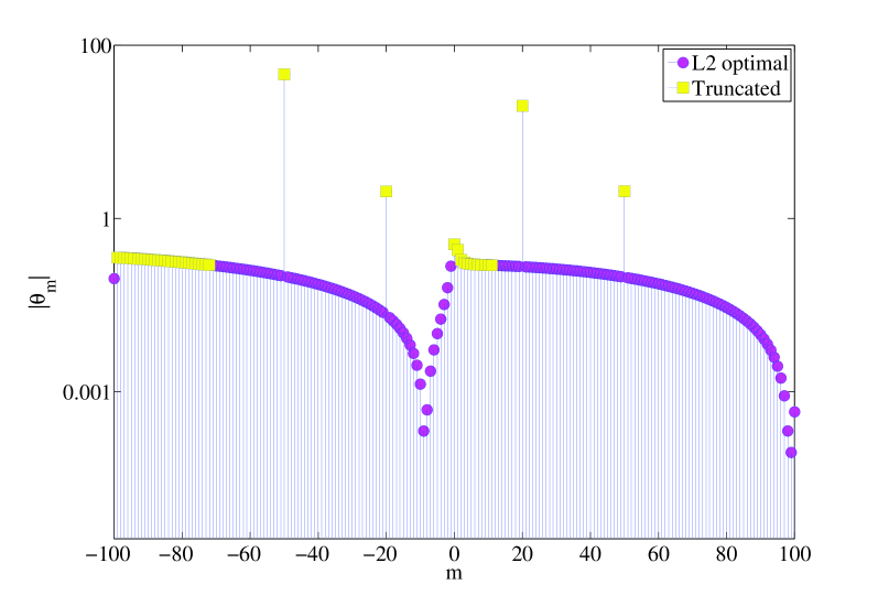
Figure 4. The absolute values of the elements of the Fourier coefficient vector ${\boldsymbol{\theta}}_{2}^{\star}$ in the $\ell^{2}$ optimal control signal $u\in V_{M}$. The squared markers show the $44$ largest coefficients which are used for a truncated vector.

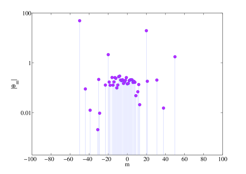
Figure 5. The absolute values of the elements of the Fourier coefficient vector ${\boldsymbol{\theta}}_{1}^{\star}$ in the $\ell^{1}\text{-}\ell^{2}$ optimal control signal $u\in V_{M}$. The $0$-valued elements are omitted. The sparsity is $\|{\boldsymbol{\theta}}_{1}^{\star}\|_{0}=44$.

Fig. 6 shows the output $y(t)$ of the system $P$ by the $\ell^{2}$ optimal control. The response is optimal in the sense that the control uses the whole sampled data on the sampling instants $t_{1},\ldots,t_{101}$. On the other hand, Fig. 7 shows the output $y(t)$ by the proposed $\ell^{1}\text{-}\ell^{2}$ optimal control.

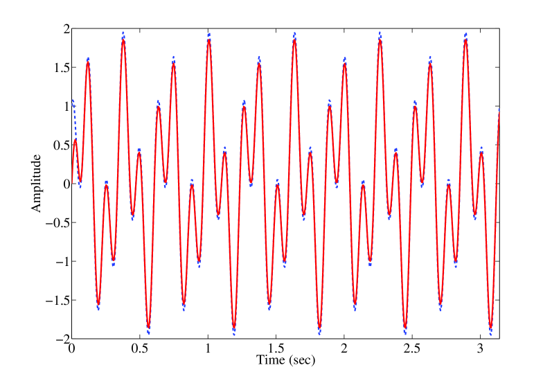
Figure 6. The reference $r(t)$ (dots) and the output $y(t)$ (solid), $t\in[0,\pi]$, by the $\ell^{2}$-optimal control

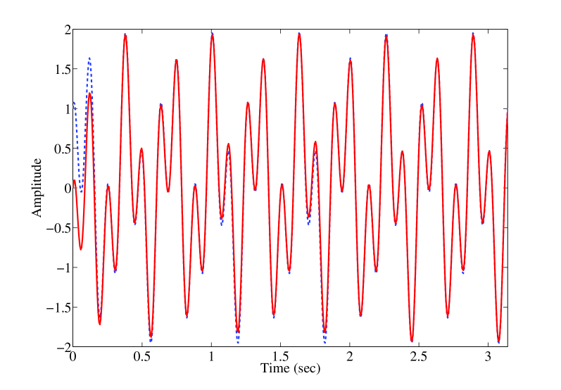
Figure 7. The reference $r(t)$ (dots) and the output $y(t)$ (solid), $t\in[0,\pi]$, by the $\ell^{1}\text{-}\ell^{2}$ optimal control

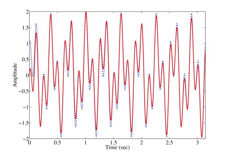
Figure 8. The reference $r(t)$ (dots) and the output $y(t)$ (solid), $t\in[0,\pi]$, by the truncated $\ell^{2}$ optimal control.

We also show the output $y(t)$ by using the $44$ largest coefficients in the $\ell^{2}$ optimal vector ${\boldsymbol{\theta}}_{2}^{\star}$ (see Fig. 4). Note that this truncated vector has the same cardinality as the $\ell^{1}\text{-}\ell^{2}$ optimal vector ${\boldsymbol{\theta}}_{1}^{\star}$. Although the proposed control signal ${\boldsymbol{\theta}}_{1}^{\star}$ was computed by only $K=67$ randomly sampled data, the output tracks the reference with quite a good performance as the $\ell^{2}$ optimal control, and better than the truncation.

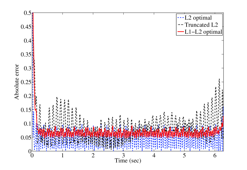
Figure 9. The tracking error $|r(t)-y(t)|$ by the $\ell^{1}\text{-}\ell^{2}$ optimal control (averaged, solid), the $\ell^{2}$ optimal control(dash), and the truncated $\ell^{2}$ optimal control (averaged, dash-dot) whose cardinality is the same as the $\ell^{1}\text{-}\ell^{2}$ optimal control.

To see the difference more precisely, we run $1000$ simulations with random sampling and compute the average of the absolute value of the tracking error $|r(t)-y(t)|$. Fig. 9 shows the result. We can see that the control performance by the proposed method is almost comparable with that by the $\ell^{2}$ method, and much better than that by the truncated $\ell^{2}$ optimal vector. Note that the average of the cardinality $\|{\boldsymbol{\theta}}_{1}^{\star}\|_{0}$ is about $57.8$, which is about $28.8\%$ of that of ${\boldsymbol{\theta}}_{2}^{\star}$.

Then we simulate for another reference signal, the step function defined by

$$r(t)=1,~{}t\in[0,2\pi].$$

The sparsity of this reference is $S_{\!r}=1$. We here assume that $K=N$ and run 1000 simulations with a random initial state ${\boldsymbol{x}}_{0}\sim{\mathcal{N}}({\boldsymbol{0}},I)$. The other parameters are the same as above. Fig. 10 shows the average of the absolute errors by the $\ell^{2}$ optimal control and the $\ell^{1}\text{-}\ell^{2}$ optimal one.

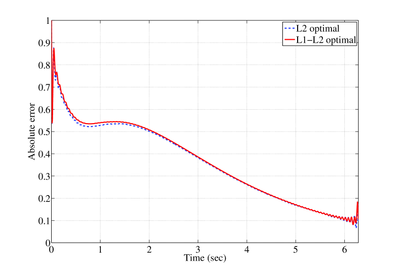
Figure 10. The average of the absolute error $|y(t)-r(t)|$ of the $\ell^{2}$ optimal control (dash) and the proposed $\ell^{1}\text{-}\ell^{2}$ optimal control (solid). The performance is comparable but the proposed control vector is much sparser.

The performance is comparable but the proposed control vector ${\boldsymbol{\theta}}_{1}^{\star}$ has the average sparsity $\|{\boldsymbol{\theta}}_{1}^{\star}\|_{0}=152.512$, which is about $76\%$ of the full vector ${\boldsymbol{\theta}}_{2}^{\star}$. That is, the proposed method can produce much sparser control vectors without much deterioration of control performance.

In conclusion, the proposed method has successfully achieved an admissible level of control performance with highly compressive sampling and sparse control signal representation.

7. Conclusion

In this paper, we have proposed a new method for remote control systems based on the compressive sampling technique. We have shown that, by assuming the sparse reference signal, the Fourier coefficients of the optimal tracking control signal can be much sparser with far fewer data than what conventional design requires. The computational cost is relatively low due to the combined use of the low rate random sampling and an efficient optimization algorithm. A theoretical result has been given for control performance analysis based on the notion of RIP. Examples have been shown that the proposed method provides a very sparse control signal without much deterioration of control performance. The sparsity of the control vector depends also on the signal subspace $V_{M}$. We leave open the problem how to select this space for a given plant $P$ and a set of reference signals.

Appendix A Proof of Lemma 1

For an input $u\in V_{M}$, the output $y(\tau)$, $\tau\in[0,T]$ is given by

$$\begin{split}y(\tau)&={\boldsymbol{c}}^{\top}\exp(\tau A){\boldsymbol{x}}_{0}+\int_{0}^{\tau}{\boldsymbol{c}}^{\top}\exp\left[(\tau-t)A\right]{\boldsymbol{b}}u(t){\mathrm{d}}t\\ &={\boldsymbol{c}}^{\top}\exp(\tau A){\boldsymbol{x}}_{0}\\ &\qquad+\sum_{m=-M}^{M}\theta_{m}\int_{0}^{\tau}{\boldsymbol{c}}^{\top}\exp\left[{(\tau-t)A}\right]{\boldsymbol{b}}\psi_{m}(t){\mathrm{d}}t\\ &={\boldsymbol{c}}^{\top}\exp(\tau A){\boldsymbol{x}}_{0}+\sum_{m=-M}^{M}\theta_{m}\int_{0}^{T}\kappa(\tau,t)\psi_{m}(t){\mathrm{d}}t\\ &={\boldsymbol{c}}^{\top}\exp(\tau A){\boldsymbol{x}}_{0}+\sum_{m=-M}^{M}\theta_{m}\langle\kappa(\tau,\cdot),\psi_{m}\rangle.\end{split}$$

Appendix B Computing inner product

To compute the matrix $G$ in (6), we have to compute the inner product $\langle\phi_{n},\psi_{m}\rangle$. This value can be easily computed by matrix exponentials [34]:

$$\begin{split}\langle\phi_{n},\psi_{m}\rangle&=\int_{0}^{T}\phi_{n}(t)\overline{\psi_{m}(t)}~{}{\mathrm{d}}t\\ &=\int_{0}^{t_{n}}{\boldsymbol{c}}^{\top}\exp\left[{(t_{n}-t)A}\right]{\boldsymbol{b}}\exp(-j\omega_{m}t){\mathrm{d}}t\\ &=[{\boldsymbol{c}}^{\top},0]\exp\left(t_{n}\begin{bmatrix}A&{\boldsymbol{b}}\\ 0&-{\mathrm{j}}\omega_{m}\end{bmatrix}\right)\begin{bmatrix}{\boldsymbol{0}}_{\nu}\\ 1\end{bmatrix},\end{split}$$

where ${\boldsymbol{0}}_{\nu}$ is the zero vector in ${\mathbb{C}}^{\nu}$.

Appendix C FISTA

We here give the algorithm of FISTA (Fast Iterative Shrinkage-Thresholding Algorithm) by [28].

Give an initial value ${\boldsymbol{\theta}}[0]\in{\mathbb{C}}^{N}$, and let $\beta[1]=1$, ${\boldsymbol{\theta}}^{\prime}[1]={\boldsymbol{\theta}}[0]$. Fix a constant $c$ such that $c>\|\Phi\|^{2}:=\lambda_{\max}(\Phi^{\top}\Phi)$. Execute the following iteration:

$$\begin{split}{\boldsymbol{\theta}}[j]&=\mathcal{S}_{2\mu_{1}/c}\left(\frac{1}{c}\Phi^{\top}({\boldsymbol{\alpha}}-\Phi{\boldsymbol{\theta}}^{\prime}[j])+{\boldsymbol{\theta}}^{\prime}[j]\right),\\ \beta[j+1]&=\frac{1+\sqrt{1+4\beta[j]^{2}}}{2},\\ {\boldsymbol{\theta}}^{\prime}[j+1]&={\boldsymbol{\theta}}[j]+\frac{\beta[j]-1}{\beta[j+1]}({\boldsymbol{\theta}}[j]-{\boldsymbol{\theta}}[j-1]),\\ j&=1,2,\ldots,\end{split}$$

where the function $\mathcal{S}_{2\mu_{1}/c}$ is defined for ${\boldsymbol{\theta}}=[\theta_{1},\ldots,\theta_{N}]^{\top}$ by

$$\mathcal{S}_{2\mu_{1}/c}({\boldsymbol{\theta}}):=\begin{bmatrix}\mathrm{sgn}(\theta_{1})(|\theta_{1}|-2\mu_{1}/c)_{+}\\ \vdots\\ \mathrm{sgn}(\theta_{N})(|\theta_{N}|-2\mu_{1}/c)_{+}\end{bmatrix},$$

where $\mathrm{sgn}(z):=\exp({\mathrm{j}}\angle z)$ for $z\in{\mathbb{C}}$, and $(x)_{+}:=\max\{x,0\}$ for $x\in{\mathbb{R}}$.

Appendix D Proof of Lemma 2

Let ${\boldsymbol{\theta}}_{1}^{\star}(\mu_{1})$ be the minimizer of the $\ell^{1}\text{-}\ell^{2}$ cost function $J_{1}({\boldsymbol{\theta}})$ with the regularization parameter $\mu_{1}>0$. We denote $\tilde{{\boldsymbol{\theta}}}^{\star}_{1}(\mu_{1})$ the reduced dimensional vector built upon the nonzero components of ${\boldsymbol{\theta}}_{1}^{\star}(\mu_{1})$. Similarly, $\tilde{\Phi}$ denotes the associated columns in the matrix $\Phi$. By the discussion in [35, Section IV], for sufficiently small $\mu_{1}$ such that $\mu_{1}\in(0,\mu_{0})$, the nonempty interval in which $\mathrm{sgn}(\tilde{{\boldsymbol{\theta}}}^{\star}_{1}(\mu_{1}))=\mathrm{sgn}(\tilde{\Phi}^{+}{\boldsymbol{\alpha}})$, the $\ell^{1}\text{-}\ell^{2}$ optimal ${\boldsymbol{\theta}}^{\star}_{1}(\mu_{1})$ is also the solution of

$$\min_{\boldsymbol{\theta}}\|{\boldsymbol{\theta}}\|_{1}~{}\text{subject to}~{}\|\Phi{\boldsymbol{\theta}}-{\boldsymbol{\alpha}}\|_{2}\leq\epsilon_{2},$$

where $\epsilon_{2}=\|\Phi{\boldsymbol{\theta}}^{\star}_{1}(\mu_{1})-{\boldsymbol{\alpha}}\|_{2}$. Then by the assumption $\delta_{2S}<\sqrt{2}-1$, we have [36]

$$\begin{split}\|{\boldsymbol{\theta}}^{\star}_{1}-{\boldsymbol{\theta}}^{\star}\|_{2}&\leq C_{0}\frac{\|{\boldsymbol{\theta}}^{\star}-{\boldsymbol{\theta}}^{\star}_{[S]}\|_{1}}{\sqrt{S}}+C_{1}\epsilon_{2}\\ &\leq C_{0}\frac{\epsilon_{1}}{\sqrt{S}}+C_{1}\epsilon_{2}.\end{split}$$

References

- [1] J.C. Lee, “Hacking the Nintendo Wii remote,” IEEE Pervasive Computing, vol.7, pp.39–45, Jul. - Sep. 2008.
- [2] T. Kubota, T. Hashimoto, J. Kawaguchi, M. Uo, and K. Shirakawa, “Guidance and navigation of Hayabusa spacecraft for asteroid exploration and sample return mission,” Proc. SICE-ICASE International Joint Conference, pp.2793–2796, Oct. 2006.
- [3] C. Sayers, Remote Control Robotics, Springer, 1999.
- [4] A.F.T. Winfield and O.E. Holland, “The application of wireless local area network technology to the control of mobile robots,” Microprocessors and Microsystems, vol.23, pp.597–607, Mar. 2000.
- [5] R.C. Luo and T.M. Chen, “Development of a multibehavior-based mobile robot for remote supervisory control through the Internet,” IEEE/ASME Trans. Mechatron., vol.5, no.4, Dec. 2000.
- [6] E.J. Candes, “Compressive sampling,” Proc. International Congress of Mathematicians, vol.3, pp.1433–1452, Aug. 2006.
- [7] E.J. Candes and M.B. Wakin, “An introduction to compressive sampling,” IEEE Signal Processing Magazine, vol.25, no.2, pp.21–30, Mar. 2008.
- [8] D.L. Donoho, “Compressed sensing,” IEEE Trans. Information Theory, vol.52, no.4, pp.1289–1306, Apr. 2006.
- [9] A.M. Bruckstein, D.L. Donoho, and M. Elad, “From sparse solutions of systems of equations to sparse modeling of signals and images,” SIAM Rev., vol.51, no.1, pp.34–81, 2009.
- [10] C.E. Shannon, “Communication in the presence of noise,” Proc. IRE, vol.37, no.1, pp.10–21, Jan. 1949.
- [11] M. Unser, “Sampling — 50 years after Shannon,” Proceedings of the IEEE, vol.88, no.4, pp.569–587, Apr. 2000.
- [12] J.L. Starck, F. Murtagh, and J.M. Fadili, Sparse Image and Signal Processing, Cambridge University Press, 2010.
- [13] G.K. Wallace, “The JPEG still picture compression standard,” Comm. ACM, vol.34, no.4, pp.30–44, Apr. 1991.
- [14] E. Candes and T. Tao, “The Dantzig selector: statistical estimation when is much larger than ,” The Annals of Statistics, vol.35, no.6, pp.2313–2351, 2007.
- [15] S. Sarvotham, D. Baron, and R.G. Baraniuk, “Measurements vs. bits: Compressed sensing meets information theory,” Allerton Conference on Communication, Control and Computing, Sep. 2006.
- [16] R. Calderbank, S. Jafarpour, and R. Schapire, “Compressed learning: Universal sparse dimensionality reduction and learning in the measurement domain,” tech. rep., 2009.
- [17] S. Mallat, A Wavelet Tour of Signal Processing, Elsevier, 2009.
- [18] M. Elad, Sparse and Redundant Representations, Springer, 2010.
- [19] S. Bhattacharya and T. Başar, “Sparsity based feedback design: a new paradigm in opportunistic sensing,” Proc. of American Control Conference, pp.3704–3709, Jul. 2011.
- [20] M. Nagahara and D.E. Quevedo, “Sparse representations for packetized predictive networked control,” IFAC 18th World Congress, pp.84–89, Aug. 2011.
- [21] M. Nagahara, D.E. Quevedo, J. Østergaard, T. Matsuda, and K. Hayashi, “Sparse command generator for remote control,” 9th IEEE International Conf. Control and Automation, Dec. 2011. (to be presented).
- [22] I. Kontoyiannis, “Pointwise redundancy in lossy data compression and universal lossy data compression,” IEEE Trans. Inf. Theory, vol.46, no.1, pp.136 –152, Jan. 2000.
- [23] J. Tropp, J. Laska, M. Duarte, J. Romberg, and R. Baraniuk, “Beyond Nyquist: Efficient sampling of sparse bandlimited signals,” IEEE Trans. Information Theory, vol.56, no.1, pp.520–544, Jan. 2010.
- [24] M. Zibulevsky and M. Elad, “L1-L2 optimization in signal and image processing,” IEEE Signal Processing Magazine, vol.27, pp.76–88, May 2010.
- [25] R. Tibshirani, “Regression shrinkage and selection via the LASSO,” J. R. Statist. Soc. Ser. B, vol.58, no.1, pp.267–288, 1996.
- [26] S.S. Chen, D.L. Donoho, and M.A. Saunders, “Atomic decomposition by basis pursuit,” SIAM J. Sci. Comput., vol.20, no.1, pp.33–61, 1998.
- [27] I. Daubechies, M. Defrise, and C. De-Mol, “An iterative thresholding algorithm for linear inverse problems with a sparsity constraint,” Comm. Pure Appl. Math., vol.57, no.11, pp.1413–1457, Aug. 2004.
- [28] A. Beck and M. Teboulle, “A fast iterative shrinkage-thresholding algorithm for linear inverse problems,” SIAM J. Imaging Sciences, vol.2, no.1, pp.183–202, Jan. 2009.
- [29] S. Sun, M.B. Egerstedt, and C.F. Martin, “Control theoretic smoothing splines,” IEEE Trans. Automat. Contr., vol.45, no.12, pp.2271–2279, Dec. 2000.
- [30] H.P. Hsu, Fourier Analysis, Simon & Schuster, 1967.
- [31] B. Schölkopf and A.J. Smola, Learning with Kernels, The MIT Press, 2002.
- [32] M. Rudelson and R. Vershynin, “On sparse reconstruction from Fourier and Gaussian measurements,” Comm. Pure Appl. Math., vol.61, no.8, pp.1025–1045, Aug. 2008.
- [33] N. Young, An Introduction to Hilbert Space, Cambridge University Press, 1988.
- [34] C.F.V. Loan, “Computing integrals involving the matrix exponential,” IEEE Trans. on Automatic Control, vol.23, no.3, pp.395–404, Jun. 1978.
- [35] J.J. Fuchs, “On sparse representations in arbitrary redundant bases,” IEEE Trans. Information Theory, vol.50, no.6, pp.1341–11344, Jun. 2004.
- [36] E. Candes, J. Romberg, and T. Tao, “Stable signal recovery from incomplete and inaccurate measurements,” Comm. Pure Appl. Math., vol.59, no.8, pp.1207–1223, Aug. 2006.