An Algorithm on Multivariate Interpolation for Cartesian Grid Complex Boundary Problems

Abstract

We present a simple algorithm to select multivariate interpolation stencil with a Cartesian grid. We show its applicability by using this algorithm in the embedded boundary method for solving the elliptic interface problem.

1 Introduction

In order to solve Cartesian grid complex boundary problems, we frequently need to select stencil from the Cartesian grid points for multivariate interpolation to approximate some function or its derivatives. Generally, second degree polynomial would be accurate enough for many applications. In two dimension ($2D$), an arbitrary second degree polynomial has six unknown coefficients and it is comparatively easy to find a stencil with six Cartesian grid points which can uniquely determine the polynomial. However, it is not so easy to do so in three dimension (3D) for a second degree polynomial with ten unknown coefficients which requires ten grid points.

To approximate solution flux (or function derivative), Johansen et al [3] uses seven grid points to compute a second order flux in $2D$, and Schwartz et al [6] uses $19$ Cartesian grid points to compute a second order flux in $3D$. When we use these fluxes to approximate the elliptic problem, the matrix has large non-zero entry and thus requires more time to obtain convergence. Another difficulty is that there might not be enough grid points available to select from for complex boundary.

Guenther et al [2] gives a simple and clever way to select stencil for interpolation in higher dimension. Gasca et al [1] reviews the polynomial interpolation algorithms in several variables. With some modification of the idea in [2], we present a simple algorithm to select stencil for multivariate interpolation in $2D$ and $3D$.

In section 2, we give the algorithms to select the stencil and also the rationale why the stencil selected can be used to uniquely determine an arbitrary second degree polynomial. In section 3, we apply this algorithm in our embedded boundary method (EBM) [8] to solve an elliptic interface problem. Finally, we give the conclusion.

2 Methods

2.1 2D Interpolation

Our $2D$ stencil selection algorithm is a modification of the algorithm presented in [8]. For simplicity, we only select grid points which are at most two grid block away from the starting grid point $(i,j)$ as shown in Fig 1. As in Wang et al[8], we classify the candidate grid points into different group of neighbors.

• Zeroth layer neighbor: simply the grid point $(i,j)$ around which we want to select candidate grid points for interpolation.

• First layer neighbor: grid points with grid index $(\hat{i},\hat{j})$ satisfying

  $$max(\left|\hat{i}-i\right|,\left|\hat{j}-j\right|)=1.$$

Thus, the first layer grid points include $(i-1,j-1)$, $(i,j-1)$, $(i+1,j-1)$, $(i-1,j)$, $(i+1,j)$, $(i-1,j+1)$, $(i,j+1)$.

• Second layer neighbor: grid points with grid index $(\hat{i},\hat{j})$ satisfying

  $$max(\left|\hat{i}-i\right|,\left|\hat{j}-j\right|)=2.$$

For convenience, we separate the second layer neighbors into four overlapping sets as in Fig 1: west, east, south, and north neighbors.

• Consecutive grid points: consecutive grid points in a given layer.

To find 6 points for quadratic polynomial interpolation, Wang et al[8] uses the following algorithm: 1) select grid point $(i,j)$; 2) select two consecutive grid points from the first layer neighbors; 3) select three consecutive grid points from the second layer neighbors. However, it is later realized that one configuration (and its symmetric configurations) gives a singular matrix when it is used to determine the unknown coefficients for a quadratic polynomial as in Fig 2.

Our improved algorithm to select candidate cells for quadratic polynomial interpolation in $2D$ is the following:

1. always select grid point $(i,j$).

2. select two consecutive grid points from the first layer neighbors.

3. select one direction, say south, and select three grid points from the second layer south neighbors.

Note that the first two steps of the above algorithm guarantee that the three selected points are not on a straight line.

In the following, we prove that we can find a unique quadratic polynomial using the above algorithm.

Proof. For simplicity, we assume that we select south direction in the third step. An arbitrary $2D$ quadratic polynomial can be written as

$$f(x,y)=a_{0}+a_{10}x+a_{01}y+a_{20}x^{2}+a_{11}xy+a_{02}y^{2}$$

which can also be rewritten as

$$f(x,y)=a_{0}+a_{10}x+a_{20}x^{2}+y(a_{01}+a_{11}x+a_{02}y).$$ (1)

We put the origin of the $2D$ coordinate system at the grid point $(i,j-2)$. Thus the south neighbor grid points are on the $x$ coordinate. Now we need to determine the unknown coefficients in equation 1. Note that

$$f(x,0)=a_{0}+a_{10}x+a_{20}x^{2}.$$

There are three unknown coefficients. We can select three grid points from the second layer south neighbors. After $a_{0}$, $a_{10}$, and $a_{20}$ are determined, we have

$$f(x,y)-(a_{0}+a_{10}x+a_{20}x^{2})=y(a_{01}+a_{11}x+a_{02}y).$$

When $y\neq 0$, we have

$$\left.\frac{f(x,y)-(a_{0}+a_{10}x+a_{20}x^{2})}{y}\right|_{y\neq 0}=a_{01}+a_{11}x+a_{02}y.$$

The right hand side of the above equation is a first deegree linear polynomial with three unknown coefficients. It can be uniquely determined by using the three grid points selected by the first two steps of the algorithm since these three points are not on a straight line. Thus we have proved that the algorithm can uniquely determine a quadratic polynomial in $2D$. $\blacksquare$

Note that we can easily extend the above proof to modify our algorithm to find stencil for higher order polynomials. An arbitrary third degree polynomial can be written as

$$f(x,y) = a_{0}+a_{10}x+a_{01}y+a_{20}x^{2}+a_{11}xy+a_{02}y^{2}+$$

$$a_{30}x^{3}+a_{21}x^{2}y+a_{12}xy^{2}+a_{03}y^{3}$$

which can be rearranged as

$$f(x,y) = a_{0}+a_{10}x+a_{20}x^{2}+a_{30}x^{3}+$$

$$y(a_{01}+a_{11}x+a_{21}x^{2}+a_{02}y+a_{12}xy+a_{03}y^{2}).$$

Suppose that we have select the south direction to select candidate grid points on the third layer south neighbors. As before, we can set the origin of the coordinate system at the center of the third layer south neighbors. Selecting four cells from the third layer south neighbors, we can uniquely determine $a_{0}$, $a_{10}$, $a_{20}$, and $a_{30}$. Then we have

$$\left.\frac{f(x,y)-(a_{0}+a_{10}x+a_{20}x^{2}+a_{30}x^{3})}{y}\right|_{y\neq 0}=(a_{01}+a_{11}x+a_{21}x^{2}+a_{02}y+a_{12}xy+a_{03}y^{2})$$

where the right hand side is a quadratic polynomial and it can be determined using the algorithm we have presented above using the grid point $(i,j)$ and its first and second layer neighbors.

Figure 1: 2D Stencil

.

Figure 2: 2D Stencil with configuration leading to a singular matrix. The selected grid points are denoted using a circle at the cell center

2.2 3D Interpolation

For a grid point $(i,j,k$), it has 6 directions: west, east in the x coordinate direction; south, north in the y coordinate direction; and down, up in the z coordinate direction.

The algorithm for $2D$ can be easily extended to $3D$ as the following:

1. always select grid point $(i,j,k$).

2. select one direction, say east, and select three consecutive grid points which are not on a straight line from the first layer east neighbors.

3. select one direction, say down, and select six grid points from the second layer down neighbors.

Note that the first two steps of the above algorithm guarantee that the four selected grid points are not on a plane. Step 2 can be done using the first two steps of the $2D$ algorithm when we consider the first layer east neighbors as a $2D$ plane. Similarly, step 3 above can be done using the $2D$ algorithm when we consider the second layer down neighbors as a $2D$ plane.

Now we prove that the above algorithm can be used to select stencil to uniquely determine a quadratic polynomial uniquely in $3D$.

Proof. The proof is similar to the proof in $2D$. An arbitrary $3D$ quadratic polynomial can be written as

$$f(x,y,z) = a_{0}+a_{100}x+a_{010}y+a_{001}z+$$

$$a_{200}x^{2}+a_{110}xy+a_{101}xz+$$

$$a_{020}y^{2}+a_{011}yz+a_{002}z^{2}$$

which can also be rearranged as

$$f(x,y,z) = a_{0}+a_{10}x+a_{01}y+a_{20}x^{2}+a_{11}xy+a_{02}y^{2}+$$

$$z(a_{001}+a_{101}x+a_{011}y+a_{002}z)$$

Assuming that we select the down direction to select six grid points from the second layer neighbors. Set the origin at grid point $(i,j,k-2)$. When $z=0$, we have

$$f(x,y,0) = a_{0}+a_{10}x+a_{01}y+a_{20}x^{2}+a_{11}xy+a_{02}y^{2}$$

where the unknown coefficients can be determined using the $2D$ algorithm to select six grid points in the second layer down neighbors. After $a_{0}$, $a_{10}$, $a_{01}$, $a_{20}$, $a_{11}$, and $a_{02}$ have been determined, we have

$$\left.\frac{f(x,y,z)-a_{0}+a_{10}x+a_{01}y+a_{20}x^{2}+a_{11}xy+a_{02}y^{2}}{z}\right|_{z\neq 0}=a_{001}+a_{101}x+a_{011}y+a_{002}z$$

Now, we only need to determine the unknown coefficients from the right hand side of the above formula. Since it is a linear polynomial in three variables, we can easily know that the first two steps of the $3D$ algorithm can be used to select four grid points (which are not on the second layer down neighbor plane) which can be used to uniquely determine the four unknown coefficients. Thus we have proved that the algorithm can uniquely determine a quadratic polynomial in 3D. $\blacksquare$

Similarly as in $2D$, we can easily extend the algorithm to select the stencil for higher order polynomials in 3D or extend it to higher dimension.

3 Application

We now use the algorithm to solve an elliptic interface problem in the Cartesian coordinate. For more detail, refer to [8, 7, 5].

An elliptic interface problem is a special elliptic problem with an internal interface:

$$\nabla\centerdot\frac{\nabla p}{\rho}=f$$ (2)

where $\rho$ is a piecewise continuous function with jump across the internal interface and $f$ is a given function which is continuous inside each part of the domain. For the interior interface, we have the following two jump conditions:

$$[p]=J_{1}(\mathbf{x}),$$ (3)

$$[\frac{1}{\rho}\frac{\partial p}{\partial n}]=J_{2}(\mathbf{x}),$$ (4)

where $J_{1}$ and $J_{2}$ are given functions of the spatial variables [4]. The embedded boundary method [8, 7, 5] uses a Cartesian mesh and the mesh cells are classified into four types: external, internal, boundary, and partial cells depending on whether there is an interior interface or exterior interface cutting through the cells. The treatment of a boundary cell is similar to that of an partial cells but much simpler. For an partial cell (see Fig 3, cell $(i,j)$), it consists of two parts separated by a cell interface.

We store four unknowns at such a partial cell: two at the cell center and two at the cell interface center for the two different components. By using the elliptic equation 2 for the two partial parts of the cell and the two jump conditions, we could set up four algebraic equations. To discretize equation 4, for example, we have

$$\left.\frac{1}{\rho}\frac{\partial p}{\partial n}\right|_{intfc,a}-\left.\frac{1}{\rho}\frac{\partial p}{\partial n}\right|_{intfc,b}=J_{2}(x)$$

where $\left.\frac{1}{\rho}\frac{\partial p}{\partial n}\right|_{intfc,a}$ is the flux calculated by polynomial interpolation selecting cells belonging to component $a$ only. When we select cells for interpolation using the $3D$ algorithm presented in the previous section, it is best to try to find candidate cells in the normal direction.

Please refer to [8, 7, 5] for more detail.

We use the method of manufactured solutions to verify our EBM implementation for the elliptic interface problem in the Cartesian coordinate. The computational domain is $[0,3]\times[0,3]\times[0,3]$. The interface position is a sphere, given as

$$\sqrt{(x-1.5)^{2}+(y-1.5)^{2}+(z-1.5)^{2}}=1.$$

We use $\rho_{d}=1$ inside the sphere and $\rho_{o}=0.001$ out side. The exact solution is

$$p(x,y,z)=\begin{cases}(x^{2}+y^{2}+z^{2})^{\frac{3}{2}},&\sqrt{(x-1.5)^{2}+(y-1.5)^{2}+(z-1.5)^{2}}<1.\\ 0.001\times(x^{2}+y^{2}+z^{2})^{\frac{3}{2}}+(1-\frac{1}{10})\times\frac{1}{8},&other\end{cases}$$

We substitute the exact solution into the elliptic equation 2 to calculate the right hand side $f$. Table 1 shows the mesh convergence for the this problem. From the table, we can see that the method is second order accurate in the $L_{\infty}$ norm.

Table 1: Mesh Convergence Study for the Elliptic Interface Problem

Mesh Size	$L_{\infty}$ Error
10x10x10	0.19727211
20x20x20	0.05673376
40x40x40	0.01312201
80x80x80	0.00341078

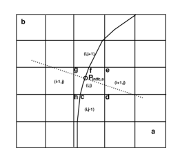
Figure 3: Stencil for the discretization of a partial cell

4 Conclusion

In this paper, we present a simple algorithm to select Cartesian grid stencil for the multivariate interpolation in $2D$ and $3D$. The correctness proof has been given using a constructive method. We show its applicability by using this algorithm in the embedded boundary method for solving the elliptic interface problem.

It should be noted that the algorithm given is not unique. It is easy to adopt the constructive method to create other algorithms for selecting interpolation stencil for different needs. For example, we do not need to restrict ourselves to select candidate grid points only in the first and second layer neighbors.

References

- [1] Mariano Gasca and Thomas Sauer. Polynomial interpolation in several variables. Advances in Computational Mathematics, 12:377–410, 2000.
- [2] R. B. Guenther and E. L. Roetman. Some observations on interpolation in higher dimensions. Mathematics of Computation, 24(111):517–522, 1970.
- [3] H. Johansen and P. Colella. A cartesian grid embedding boundary method for poisson’s equation on irregular domains. J. Comput. Phys., 147:60–85, 1998.
- [4] R.J. LeVeque and Z.L. Li. The immersed interface method for elliptic equations with discontinuous coefficients and singular sources. SIAM J. Numer. Anal., 31:1019–1044, 1994.
- [5] P. Schwartz, M. Barad, P. Colella, and T. Ligocki. A Cartesian grid embedded boundary method for the heat equation and Poisson’s equation in three dimensions. J. Comput. Phys., 211:531–550, 2006.
- [6] Peter Schwartz, Michael Barad, Phillip Colella, and Terry Ligocki. A cartesian grid embedded boundary method for the heat equation and poisson’s equation in three dimensions. J. Comput. Phys., 211:531–550, 2006.
- [7] S. Wang, J. Glimm, R. Samulyak, X. Jiao, and C. Diao. The embedded boundary method for two phase incompressible flow. 2013. arXiv:1304.5514.
- [8] Shuqiang Wang, Roman V Samulyak, and Tongfei Guo. An embedded boundary method for elliptic and parabolic problems with interfaces and application to multi-material systems with phase transitions. Acta Mathematica Scientia, 30B(2).