3D Volume Calculation For the Marching Cubes Algorithm in Cartesian Coordinates

Abstract

From a scalar field defined at the corner of a cube, an isosurface can be extracted using the Marching Cube algorithm. The isosurface separates the cell into two or more partial cells. A similar situation arises when an material interface in the Front Tracking method cuts through the computational cells. A popular method to calculate the volumes of the partial cells is to first partition the cells into tetrahedra and then sum together the volumes of the tetrahedra for the corresponding partial cells. In this paper, the divergence theorem is used to calculate the volumes of the partial cells generated by the Marching Cubes algorithm. This method is both more robust and efficient compared with the tetrahedralization approach.

1 Introduction

The Marching Cubes algorithm [6] was developed to reconstruct the interface using the volumetric data. The isosurface separates the cell into two or more partial cells. A similar situation arises when an material interface in the Front Tracking method cuts through the computational cells. Most of the publications are concerning on how to deal with interface reconstructions, while only few papers exists to show how to calculate the partial volumes enclosed by the interface. Current volume calculation methods [5, 4] often first tetrahedralize the partial volumes and then calculate the volume using the tetrahedra. This approach is difficult to write computer code to deal with all possible cases. An alternative method to the Marching Cubes algorithm is the generalized Marching Cubes method [2] which first partitions the cubic cell into tetrahedra, and then uses the generalized Marching Cubes method on the tetrahedra [2] to recover the interface, leading to few cases compared with the Marching Cubes algorithm. However, the disadvantage of using this approach to calculate the partial volumes is that we need crossing information on the cell face diagonals and the main cube diagonal which might be difficult to obtain. In this paper, we show how to calcalute the cell partial volumes by using the divergence theorm. This approach seems to be much more robust and computing efficient than the other approach. It is also very easy to be coded.

As applications of this algorithm, we can/have used it in our embedded boundary method (a finite volume method) coupled with the Front Tracking method for solving the elliptic/parabolic interface problem [12], two-phase incompressible flow [9], and magnetohydrodynamic flows [3].

2 Method

The general idea of using the divergence theorem to calculate the volume is very simple. The divergence theorem is

$$\int_{\Omega}\nabla\cdot\overrightarrow{f}dv=\oint_{\partial\Omega}\overrightarrow{n}\cdot\overrightarrow{f}ds.$$ (1)

If we can find a vector $\overrightarrow{f}$ such that

$$\nabla\cdot\overrightarrow{f}=a$$

where $a$ is a constant, then we have

$$\int_{\Omega}adv=\oint_{\partial\Omega}\overrightarrow{n}\cdot\overrightarrow{f}ds$$

or

$$Volume(\Omega)=\int_{\Omega}dv=\frac{\oint_{\partial\Omega}\overrightarrow{n}\cdot\overrightarrow{f}ds}{a}$$

2.1 Volume Calculations in Cartesian Coordinate

In a Cartesian coordinate, the divergence operator is defined as

$$\nabla\cdot\overrightarrow{f}=\frac{\partial f_{x}}{\partial x}+\frac{\partial f_{y}}{\partial y}+\frac{\partial f_{z}}{\partial z}$$

where $\overrightarrow{f}=(f_{x},f_{y},f_{z})^{T}$.

To calculate the volume of the domain $\Omega$, we can let $\overrightarrow{f}=(x,y,z)^{T}$ (which is not unique) and then we have

$$\int_{\Omega}\frac{\partial x}{\partial x}+\frac{\partial y}{\partial y}+\frac{\partial z}{\partial z}dv = \oint_{\partial\Omega}\overrightarrow{n}\cdot\overrightarrow{f}dS$$

$$\int_{\Omega}3dv = \oint_{\partial\Omega}\overrightarrow{n}\cdot\overrightarrow{f}dS$$

Therefore, we can calculate the volume using the surface integration

$$Volume(\Omega)=\int_{\Omega}dv=\frac{\int_{\partial\Omega}\overrightarrow{n}\cdot\overrightarrow{f}dS}{3}.$$ (2)

Thus, if the domain boundary $\partial\Omega$ consists of triangle meshs in the cartesian coordinate, we only need to use second order accuarate quadrature rule to obtain the exact volume.

2.2 Templates and Coding

In this paper, we use the $23$ unique cube configurations (or cases) in [7] as the $15$ cube configurations in the original Marching Cubes algorithm [6] has consistency issue [7].

Figure 1 shows the vertex, edge and face labeling scheme which is different from [7]. Note that we use a two letter word of pattern $v\bullet$ to denote the vertex labeling and a two letter word of pattern $e\bullet$ to denote the edge labeling. This kind of labeling makes it easy to write the code to calculate the volume of the cubes since we can define those two letter words as some constants and use them as the indices of the coordinate arrays. The six faces of the cube are labeled as $W$ for West (with vertex $v0,$$v3$, $v7$, $v4$), $E$ for East (with vertex $v1,$$v2$, $v6$, $v5$), $S$ for South (with vertex $v0,$ $v1$, $v5$, $v4$), $N$ for North (with vertex $v3,$$v2$, $v6$, $v7$), $D$ for Down (with vertex $v0,$$v1$, $v2$, $v3$), and $U$ for Upper (with vertex $v4,$$v5$, $v6$, $v7$). On each vertex, the componet is either $0$ or $1$. For component $1$ vertex, we draw a circle on the vertex.

To calculate the partial volumes for a cube with two different components, we calculate the volume for one of the components first, say $Volume_{1}$. Then we use the total volume of the cube to calculate the volume for the other component:

$$Volume_{0}=Volume_{total}-Volume_{1}$$

In order to calculate the volume using the surface integration in equation (2), we need to find a closed surface enclosing that component and the triangulation of the closed surface

For cubes with only two components, there are $2^{8}=256$ different unique configurations. Using rotation symmetry only, these $256$ cases can be rotated into $23$ unique cases [7] as shown in Figure 1-12.

For each case, we have shown in the corresponding figures the triangulation for the interface following [7] and the triangulations for the six faces. Each triangle of the triangulations consist of four letters: the first three letters are either the vertex index or the edge index, and the fourth letter denotes the position of the triangle: $I$ for triangle on the constructed interface, $W$ for the triangle on the West face, and similarly for the other letters.

For example, for case $01$ in Figure 2, the triangulations list consists of

{e0,e3,e8,I}, {v0,e8,e3,W}, {v0,e0,e8,S}, {v0,e3,e0,D}

For this case, there is only one triangle $\left\{e0,e3,e8,I\right\}$ on the interface, one triangle $\left\{v0,e8,e3,W\right\}$ on the West face, one triangle $\left\{v0,e0,e8,S\right\}$ on the South face, and one triangle $\left\{v0,e3,e0,D\right\}$ on the Down face. The four triangles make up the closed surface enclosing the domain corresponding to component $1$. Thus, to calculate the volume for component $1$ for case $01$, we only need to use the surface integration in equation 2. Note that, the surface consists of four triangles, thus the surface integration is a sum of the integrations on the four triangles, which can be calculated easily.

For another example, say case $03$ in Figure 3, the domain for component $1$ consists of two disconnected parts. In the triangulation list, we first list the triangulation for the first part, then the triangulations for the second part. In this way, we could easily calculate other values besides the total volume for each components, such as the number of the connected interfaces, the averaged interface normal, interface center, and interface area for each connected interface. If necessary, we can calculate separately the partial volumes for the disconnected part.

For case $01-16$, we list the triangulations for component $1$. For case $17-21$, we list the triangulations for component $0$ instead of component $1$ since there are less triangles due to cube faces triangulations. When we list the triangles for one connected domain, we first list the triangles on the interface, then triangles on the West, East, South, North, Down, and Upper faces.

After we have the triangulation list of the enclosing surface, the volume in equation 2 can be calculated using

$$Volume = \frac{\int_{\partial\Omega}\overrightarrow{n}\cdot\overrightarrow{f}ds}{3}$$

$$= \frac{1}{3}\sum_{T_{i}}\int_{T_{i}}\overrightarrow{n}\cdot\overrightarrow{f}ds$$

where $T_{i}$ is one of the triangle in the triangulation list. Thus, the surface integration has been divided into a sum of the integration on the triangles, which could be solved exactly using standard quadrature rule.

It is also easy to calculate the interface center, interface normal, interface area using the following formula:

$$\vec{X}_{intfcCenter} = \int_{intfc}xds$$

$$\vec{N}_{intfcNormal} = \int_{intfc}\vec{n}ds$$

$$A_{intfcArea} = \int_{intfc}ds$$

We simply use the triangulation of the interface only and then calculate these surface integrations by the sum of the triangle integration.

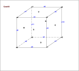
Figure 1: Case00

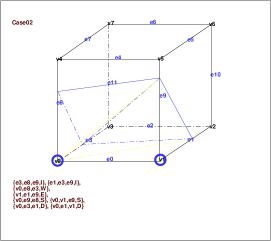
Figure 2: Case01 and Case02

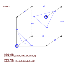
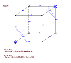
Figure 3: Case03 and Case04

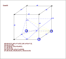
Figure 4: Case05 and Case06

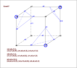
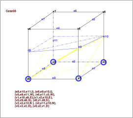
Figure 5: Case07 and Case08

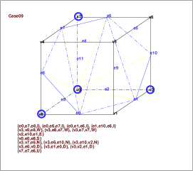
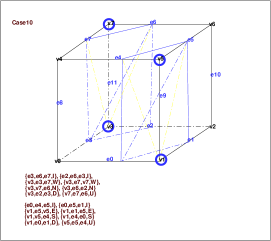
Figure 6: Case09 and Case10

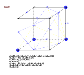
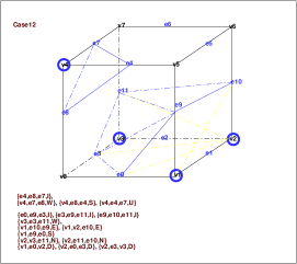
Figure 7: Case11 and Case12

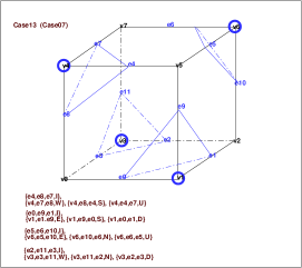
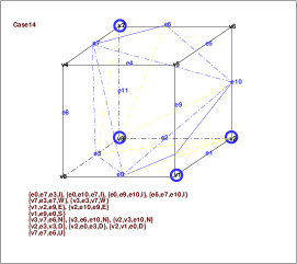
Figure 8: Case13 and Case14

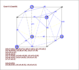
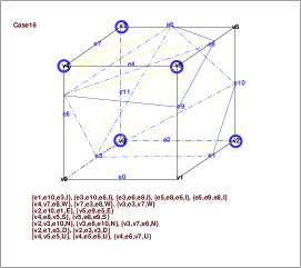
Figure 9: Case15 and Case16

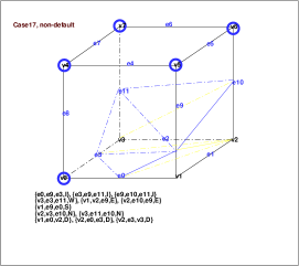
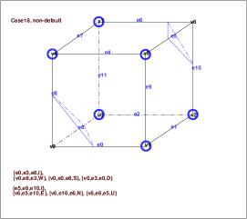
Figure 10: Case17 and Case18

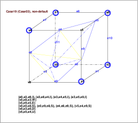
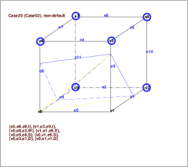
Figure 11: Case19 and Case20

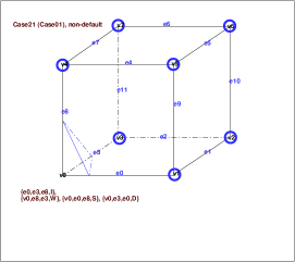
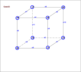
Figure 12: Case21 and Case22

3 Examples

For plane interfaces, numerical simulations show that our algorithm give exact results for the total volumes and surface areas. In the following, we use a sphere interface to do a mesh convergence study.

The computational domain is $[0,3]\times[0,3]\times[0,3]$. The interface position is a sphere, given as

$$\sqrt{(x-1.5)^{2}+(y-1.5)^{2}+(z-1.5)^{2}}=1.$$

Table 1 shows the mesh convergence study for the sphere volume and the surface area. From the table, we can see that the method is second order accurate.

Table 1: 3D Mesh Convergence Study with exact sphere volume $V=4.18879020479$ and sphere surface area $S=12.5663706144$

Mesh Size	Volume	Error	Area	Error
10x10x10	4.00416024	0.18462996479	12.27248842	0.2938821944
20x20x20	4.13823907	0.05055113479	12.48614607	0.0802245444
40x40x40	4.17534124	0.01344896479	12.54510172	0.0212688944
80x80x80	4.18536131	0.00342889479	12.56094478	0.0054258344

4 Conclusion

In this paper, we used the divergence theorem to calculate the partial cell volumes. Compared with the tetrahedralization approach, it is robust, efficient, and much easier for user to write computer code. It is also straight forward to use this method to deal with more complicated configurations [8].

The current method can be extended to Cylindrical coordinate, Spherical coordinate. These will be documented in detail in future papers [10, 11] since it is not easy to make them right.

Appendix Surface Triangles List

We list the triangulation lists for all $23$ cases which can be easily copied into C code. Note that the triangulation lists of Case $01-16$ are for component $1$ while the triangulation lists of Case $17-21$ are for component $0$.

• Case 00: N/A;

• Case 01: { {e0,e3,e8,I}, {v0,e8,e3,W}, {v0,e0,e8,S}, {v0,e3,e0,D} };

• Case 02: { {e3,e8,e9,I}, {e1,e3,e9,I}, {v0,e8,e3,W}, {v1,e1,e9,E}, {v0,e9,e8,S}, {v0,v1,e9,S}, {v0,e3,e1,D}, {v0,e1,v1,D} };

• Case 03: { {e0,e3,e8,I}, {v0,e8,e3,W}, {v0,e0,e8,S}, {v0,e3,e0,D}, {e4,e5,e9,I}, {v5,e9,e5,E}, {v5,e4,e9,S}, {v5,e5,e4,U} };

• Case 04: { {e0,e3,e8,I}, {v0,e8,e3,W}, {v0,e0,e8,S}, {v0,e3,e0,D}, {e5,e6,e10,I}, {v6,e5,e10,E}, {v6,e10,e6,N}, {v6,e6,e5,U} };

• Case 05: { {e0,e9,e3,I}, {e9,e11,e3,I}, {e9,e10,e11,I}, {v3,e3,e11,W}, {v1,v2,e9,E}, {v2,e10,e9,E}, {v1,e9,e0,S}, {v2,v3,e11,N}, {v2,e11,e10,N}, {v1,e0,v2,D}, {v2,e0,e3,D}, {v2,e3,v3,D} };

• Case 06: { {e3,e8,e1,I}, {e1,e8,e9,I}, {v0,e8,e3,W}, {v1,e1,e9,E}, {v0,e9,e8,S}, {v0,v1,e9,S}, {v0,e3,e1,D}, {v0,e1,v1,D}, {e5,e6,e10,I}, {v6,e5,e10,E}, {v6,e10,e6,N}, {v6,e6,e5,U} };

• Case 07: { {e4,e8,e7,I}, {v4,e7,e8,W}, {v4,e8,e4,S}, {v4,e4,e7,U}, {e0,e9,e1,I}, {v1,e1,e9,E}, {v1,e9,e0,S}, {v1,e0,e1,D}, {e5,e6,e10,I}, {v6,e5,e10,E}, {v6,e10,e6,N}, {v6,e6,e5,U} };

• Case 08: { {e8,e10,e11,I}, {e8,e9,e10,I}, {v0,e8,e11,W}, {v0,e11,v3,W}, {v1,e10,e9,E}, {v1,v2,e10,E}, {v0,e9,e8,S}, {v0,v1,e9,S}, {v2,v3,e10,N}, {v3,e11,e10,N}, {v0,v3,v2,D}, {v0,v2,v1,D} };

• Case 09: { {e0,e7,e8,I}, {e0,e6,e7,I}, {e0,e1,e6,I}, {e1,e10,e6,I}, {v3,v0,e8,W}, {v3,e8,e7,W}, {v3,e7,v7,W}, {v2,e10,e1,E}, {v0,e0,e8,S}, {v3,v7,e6,N}, {v3,e6,e10,N}, {v3,e10,v2,N}, {v3,e0,v0,D}, {v3,e1,e0,D}, {v3,v2,e1,D}, {v7,e7,e6,U} };

• Case 10: { {e3,e6,e7,I}, {e2,e6,e3,I}, {v3,e3,e7,W}, {v3,e7,v7,W}, {v3,v7,e6,N}, {v3,e6,e2,N}, {v3,e2,e3,D}, {v7,e7,e6,U}, {e0,e4,e5,I}, {e0,e5,e1,I}, {v1,e5,v5,E}, {v1,e1,e5,E}, {v1,v5,e4,S}, {v1,e4,e0,S}, {v1,e0,e1,D}, {v5,e5,e4,U} };

• Case 11: { {e0,e11,e8,I}, {e0,e5,e11,I}, {e0,e1,e5,I}, {e5,e6,e11,I}, {v0,e8,e11,W}, {v0,e11,v3,W}, {v2,e5,e1,E}, {v2,v6,e5,E}, {v0,e0,e8,S}, {v2,v3,e11,N}, {v2,e11,e6,N}, {v2,e6,v6,N}, {v3,e0,v0,D}, {v3,e1,e0,D}, {v3,v2,e1,D}, {v6,e6,e5,U} };

• Case 12: { {e4,e8,e7,I}, {v4,e7,e8,W}, {v4,e8,e4,S}, {v4,e4,e7,U}, {e0,e9,e3,I}, {e3,e9,e11,I}, {e9,e10,e11,I}, {v3,e3,e11,W}, {v1,e10,e9,E}, {v1,v2,e10,E}, {v1,e9,e0,S}, {v2,v3,e11,N}, {v2,e11,e10,N}, {v1,e0,v2,D}, {v2,e0,e3,D}, {v2,e3,v3,D} };

• Case 13: { {e4,e8,e7,I}, {v4,e7,e8,W}, {v4,e8,e4,S}, {v4,e4,e7,U}, {e0,e9,e1,I}, {v1,e1,e9,E}, {v1,e9,e0,S}, {v1,e0,e1,D}, {e5,e6,e10,I}, {v6,e5,e10,E}, {v6,e10,e6,N}, {v6,e6,e5,U}, {e2,e11,e3,I}, {v3,e3,e11,W}, {v3,e11,e2,N}, {v3,e2,e3,D} };

• Case 14: { {e0,e7,e3,I}, {e0,e10,e7,I}, {e0,e9,e10,I}, {e6,e7,e10,I}, {v7,e3,e7,W}, {v3,e3,e7,W}, {v1,v2,e9,E}, {v2,e10,e9,E}, {v1,e9,e0,S}, {v3,v7,e6,N}, {v3,e6,e10,N}, {v2,v3,e10,N}, {v2,e3,v3,D}, {v2,e0,e3,D}, {v2,v1,e0,D}, {v7,e7,e6,U} };

• Case 15: { {e0,e7,e8,I}, {e0,e6,e7,I}, {e0,e1,e6,I}, {e1,e10,e6,I}, {v3,v0,e8,W}, {v3,e8,e7,W}, {v3,e7,v7,W}, {v2,e10,e1,E}, {v0,e0,e8,S}, {v3,v7,e6,N}, {v3,e6,e10,N}, {v3,e10,v2,N}, {v3,e0,v0,D}, {v3,e1,e0,D}, {v3,v2,e1,D}, {v7,e7,e6,U}, {e4,e5,e9,I}, {v5,e9,e5,E}, {v5,e4,e9,S}, {v5,e5,e4,U} };

• Case 16: { {e1,e10,e3,I}, {e3,e10,e6,I}, {e3,e6,e8,I}, {e5,e8,e6,I}, {e5,e9,e8,I}, {v4,v7,e8,W}, {v7,e3,e8,W}, {v3,e3,v7,W}, {v2,e10,e1,E}, {v5,e9,e5,E}, {v4,e8,v5,S}, {v5,e8,e9,S}, {v2,v3,e10,N}, {v3,e6,e10,N}, {v3,v7,e6,N}, {v2,e1,e3,D}, {v2,e3,v3,D}, {v4,v5,e5,U}, {v4,e5,e6,U}, {v4,e6,v7,U} };

• Case 17: { {e0,e9,e3,I}, {e3,e9,e11,I}, {e9,e10,e11,I}, {v3,e3,e11,W}, {v1,v2,e9,E}, {v2,e10,e9,E}, {v1,e9,e0,S}, {v2,v3,e10,N}, {v3,e11,e10,N}, {v1,e0,v2,D}, {v2,e0,e3,D}, {v2,e3,v3,D} };

• Case 18: { {e0,e3,e8,I}, {v0,e8,e3,W}, {v0,e0,e8,S}, {v0,e3,e0,D}, {e5,e6,e10,I}, {v6,e5,e10,E}, {v6,e10,e6,N}, {v6,e6,e5,U} };

• Case 19: { {e0,e3,e9,I}, {e3,e8,e4,I}, {e3,e4,e5,I}, {e3,e5,e9,I}, {v0,e8,e3,W}, {v5,e9,e5,E}, {v0,e0,e8,S}, {e0,e9,e8,S}, {e4,e8,e9,S}, {v5,e4,e9,S}, {v0,e3,e0,D}, {v5,e5,e4,U} };

• Case 20: { {e3,e8,e9,I}, {e1,e3,e9,I}, {v0,e8,e3,W}, {v1,e1,e9,E}, {v0,e9,e8,S}, {v0,v1,e9,S}, {v0,e3,e1,D}, {v0,e1,v1,D} };

• Case 21: { {e0,e3,e8,I}, {v0,e8,e3,W}, {v0,e0,e8,S}, {v0,e3,e0,D} };

• Case 22: N/A.

Appendix Rotation List

For completeness, we list the 24 unique rotation of a cube [1] in the following:

• {0,1,2,3,4,5,6,7}, // self

• {4,5,1,0,7,6,2,3}, // opposite face: x 90

• {7,6,5,4,3,2,1,0}, // opposite face: x 180

• {3,2,6,7,0,1,5,4}, // opposite face: x 270

• {4,0,3,7,5,1,2,6}, // opposite face: y 90

• {5,4,7,6,1,0,3,2}, // opposite face: y 180

• {1,5,6,2,0,4,7,3}, // opposite face: y 270

• {3,0,1,2,7,4,5,6}, // opposite face: z 90

• {2,3,0,1,6,7,4,5}, // opposite face: z 180

• {1,2,3,0,5,6,7,4}, // opposite face: z 270

• {0,4,5,1,3,7,6,2}, // opposite vertices: v0-v6

• {0,3,7,4,1,2,6,5}, // opposite vertices: v0-v6

• {2,1,5,6,3,0,4,7}, // opposite vertices: v1-v7

• {5,1,0,4,6,2,3,7}, // opposite vertices: v1-v7

• {5,6,2,1,4,7,3,0}, // opposite vertices: v2-v4

• {7,3,2,6,4,0,1,5}, // opposite vertices: v2-v4

• {2,6,7,3,1,5,4,0}, // opposite vertices: v3-v5

• {7,4,0,3,6,5,1,2}, // opposite vertices: v3-v5

• {1,0,4,5,2,3,7,6}, // opposite lines: e0-e6

• {3,7,4,0,2,6,5,1}, // opposite lines: e3-e5

• {6,7,3,2,5,4,0,1}, // opposite lines: e2-e4

• {6,2,1,5,7,3,0,4}, // opposite lines: e1-e7

• {4,7,6,5,0,3,2,1}, // opposite lines: e8-e10

• {6,5,4,7,2,1,0,3} // opposite lines: e9-e11

References

- [1] Martin Baker. Maths - cube rotation.
- [2] Jules Bloomenthal (Editor). Introduction to Implicit Surfaces. The Morgan Kaufmann Series in Computer Graphics. Morgan Kaufmann, 1997.
- [3] T. Guo, S. Wang, and R. Samulyak. Sharp interface algorithm for large density ratio incompressible multiphase magnetohydrodynamic flows. In Proc. Comp. Science. Elsevier, 2013. accepted for publishing.
- [4] J. Hare, J. Grosh, and C. Schmitt. Volumetric measurements from an iso-surface algorithm. In Proc. SPIE, volume 3643, pages 206–210, 1999.
- [5] Dongyung Kim, Jean N. Pestieau, and James Glimm. Surfacevolume fractions and surface areas for 3-d grid cells cut by an interface. Technical Report preprint, Stony Brook AMS, 2007.
- [6] W. E. Lorensen and H. E. Cline. Marching cubes: A high resolution 3D surface construction algorithm. Computer Graphics, 21(4):163–169, 1987.
- [7] Timothy S. Newman and Hong Yi. A survery of the marching cubes algorithm. Computers & Graphics, 30:854–879, 2006.
- [8] Gregory M. Nielson. On marching cubes. IEEE Transactions on Visualization and Computer Graphics, 9(3), 2003.
- [9] S. Wang, J. Glimm, R. Samulyak, X. Jiao, and C. Diao. The embedded boundary method for two phase incompressible flow. 2013. arXiv:1304.5514.
- [10] Shuqiang Wang. An embedded boundary method for the elliptic interface problem in polar and cylindrical coordinate. in preparation, 2013.
- [11] Shuqiang Wang. An embedded boundary method for the elliptic interface problem in spherical coordinate. in preparation, 2013.
- [12] Shuqiang Wang, Roman V Samulyak, and Tongfei Guo. An embedded boundary method for elliptic and parabolic problems with interfaces and application to multi-material systems with phase transitions. Acta Mathematica Scientia, 30B(2).