Optimal Discretization of Analog Filters via Sampled-Data $H^{\infty}$ Control Theory

Abstract

In this article, we propose optimal discretization of analog filters (or controllers) based on the theory of sampled-data $H^{\infty}$ control. We formulate the discretization problem as minimization of the $H^{\infty}$ norm of the error system between a (delayed) target analog filter and a digital system including an ideal sampler, a zero-order hold, and a digital filter. The problem is reduced to discrete-time $H^{\infty}$ optimization via the fast sample/hold approximation method. We also extend the proposed method to multirate systems. Feedback controller discretization by the proposed method is discussed with respect to stability. Numerical examples show the effectiveness of the proposed method.

1 INTRODUCTION

Discretization of analog systems is a fundamental transformation in control and signal processing. Often an analog (or continuous-time) controller is designed based on standard methods such as PID control [1], and then it is implemented in digital devices after discretization. In signal processing, an analog filter is discretized to implement it on DSP (digital signal processor), an example of which is active noise control [3] where the analog model of the secondary path is discretized and used for an adaptive filter algorithm realized on DSP.

For discretization of analog filters, step-invariant transformation [2, Chap. 3] is conventionally and widely used. The term “step-invariant” comes from the fact that the discrete-time step response of the discretized filter is exactly the same as the sampled step response of the original filter. By this fact, step-invariant transformation is effective for sufficiently low-frequency signals. Another well-known discretization method is bilinear transformation, also known as Tustin’s method, which is based on the trapezoidal rule for approximating the definite integral. The following are advantages of bilinear transformation:

• stability and minimum-phase property are preserved,

• there is no error at DC (direct current) between the frequency responses of the original filter and the discretized one.

If a zero error is preferred at another frequency, one can use a prewarping technique for bilinear transformation; see [2, Sec. 3.5] for details.

Although these methods are widely used, there may lead considerable discretization errors for unexpected signals such as signals that contains high-frequency components. To solve this, we apply the sampled-data $H^{\infty}$-optimal filter design [5, 7, 12, 13] to the discretization problem. The proposed design procedure is summarized as follows:

1. give a signal generator model $F(s)$ as an analog filter for $L^{2}$ input signals,

2. set a digital system ${\mathcal{K}}$ that contains a sampler, a hold, and a digital filter (see Fig. 1),

3. construct an error system ${\mathcal{E}}$ between ${\mathcal{K}}$ and a (delayed) target analog filter $G(s)$ with signal model $F(s)$ (see Fig. 2),

4. find a digital filter in ${\mathcal{K}}$ that minimizes the $L^{2}$-induced norm (or $H^{\infty}$ norm) of the error system ${\mathcal{E}}$.

Since the error system is composed of both analog and digital systems, the optimization is an infinite dimensional one. To reduce this to a finite dimensional optimization, we introduce the fast sample/hold approximation method [4, 11]. By this method, the optimal digital filter can be effectively obtained by numerical computations.

The remainder of this article is organized as follows. In Section 2, we formulate our discretization problem as a sampled-data $H^{\infty}$ optimization. In Section 3, we review two conventional methods: step-invariant transformation and bilinear transformation. In Section 4, we give a design formula to compute $H^{\infty}$-optimal filters. In Section 5, we extend the design method to multirate systems. In Section 6, we discuss controller discretization. Section 7 presents design examples to illustrate the effectiveness of the proposed method. In Section 8, we offer concluding remarks.

Notation

Throughout this article, we use the following notation. We denote by $L^{2}[0,\infty)$ the Lebesgue space consisting of all square integrable real functions on $[0,\infty)$. $L^{2}[0,\infty)$ is sometimes abbreviated to $L^{2}$. The $L^{2}$ norm is denoted by $\|\cdot\|_{2}$. The symbol $t$ denotes the argument of time, $s$ the argument of Laplace transform, and $z$ the argument of $Z$ transform. These symbols are used to indicate whether a signal or a system is of continuous-time or discrete-time; for example, $y(t)$ is a continuous-time signal, $F(s)$ is a continuous-time system, $K(z)$ is a discrete-time system. The operator ${\mathrm{e}}^{-ls}$ with nonnegative integer $l$ denotes continuous-time delay (or shift) operator: $({\mathrm{e}}^{-ls}y)(t)=y(t-l)$. ${\mathcal{S}}_{h}$ and ${\mathcal{H}}_{h}$ denote the ideal sampler and the zero-order hold respectively with sampling period $h>0$. A transfer function with state-space matrices $A,B,C,D$ is denoted by

$$\left[\begin{array}[]{c|c}A&B\\ \hline\cr C&D\end{array}\right]:=\begin{cases}C(sI-A)^{-1}B+D,&\text{~{}(continuous-time)}\\ C(zI-A)^{-1}B+D,&\text{~{}(discrete-time)}\end{cases}$$

We denote the imaginary number $\sqrt{-1}$ by ${\mathrm{j}}$.

2 PROBLEM FORMULATION

In this section, we formulate the problem of optimal discretization.

Assume that a transfer function $G(s)$ of an analog filter is given. We suppose that $G(s)$ is a stable, real-rational, proper transfer function. Let $g(t)$ denote the impulse response (or the inverse Laplace transform) of $G(s)$. Our objective is to find a digital filter $K(z)$ in a digital system

$${\mathcal{K}}={\mathcal{H}}_{h}K{\mathcal{S}}_{h},$$

shown in Fig. 1 that mimics the input/output behavior of the analog filter $G(s)$.

Figure 1: Digital system ${\mathcal{K}}$ consisting of ideal sampler ${\mathcal{S}}_{h}$, digital filter $K(z)$, and zero-order hold ${\mathcal{H}}_{h}$ with sampling period $h$.

The digital system in Fig. 1 includes an ideal sampler ${\mathcal{S}}_{h}$ and a zero-order hold ${\mathcal{H}}_{h}$ synchronized with a fixed sampling period $h>0$. The ideal sampler ${\mathcal{S}}_{h}$ converts a continuous-time signal $u(t)$ to a discrete-time signal $v[n]$ as

$$v[n]=({\mathcal{S}}_{h}u)[n]=u(nh),\quad n=0,1,2,\dots.$$

The zero-order hold ${\mathcal{H}}_{h}$ produces a continuous-time signal $\hat{y}(t)$ from a discrete-time signal $\psi[n]$ as

$$\hat{y}(t)=\sum_{n=0}^{\infty}\psi[n]\phi(t-nh),\quad t\in[0,\infty),$$

where $\phi(t)$ is a box function defined by

$$\phi(t)=\begin{cases}1,&\text{~{}if~{}}t\in[0,h),\\ 0,&\text{~{}otherwise.}\end{cases}$$

The filter $K(z)$ is designed to produce a continuous-time signal $\hat{y}$ after the zero-order hold ${\mathcal{H}}_{h}$ that approximates the delayed output

$$y(t)=(g\ast u)(t-l)=\int_{0}^{t-l}g(\tau)u(t-l-\tau)d\tau$$

of an input $u$. A positive delay time $l$ may improve the approximation performance when $l$ is large enough as discussed in e.g., [7, 12]. We here assume $l$ is an integer multiple of $h$, that is, $l=mh$, where $m$ is a nonnegative integer. Then, to avoid a trivial solution (i.e., $K(z)=0$), we should assume some a priori information for the inputs. As used in [7, 12], we adopt the following signal subspace of $L^{2}[0,\infty)$ to which the inputs belong:

$$FL^{2}:=\left\{Fw:w\in L^{2}[0,\infty)\right\},$$

where $F$ is a linear system with a stable, real-rational, strictly proper transfer function $F(s)$. This transfer function, $F(s)$, defines the analog characteristic of the input signals in the frequency domain.

In summary, our discretization problem is formulated as follows:

Problem 1

Given target filter $G(s)$, analog characteristic $F(s)$, sampling period $h$, and delay step $m$, find a digital filter $K(z)$ that minimizes

$$\begin{split}J&=\sup_{w\in L^{2},\,\|w\|_{2}=1}\left\|\left({\mathrm{e}}^{-mhs}G-{\mathcal{H}}_{h}K{\mathcal{S}}_{h}\right)Fw\right\|_{2}\\ &=\left\|\left({\mathrm{e}}^{-mhs}G-{\mathcal{H}}_{h}K{\mathcal{S}}_{h}\right)F\right\|_{\infty}.\end{split}$$ (1)

The corresponding block diagram of the erros system

$${\mathcal{E}}:=\left({\mathrm{e}}^{-mhs}G-{\mathcal{H}}_{h}K{\mathcal{S}}_{h}\right)F$$ (2)

is shown in Fig. 2.

Figure 2: Error system ${\mathcal{E}}$.

3 STEP-INVARIANT AND BILINEAR METHODS

Before solving Problem 1, we here briefly review two conventional discretization methods, namely step-invariant transformation and bilinear transformation [2].

3.1 Step-invariant transformation

The step-invariant transformation $K_{\mathrm{d}}$ of a continuous-time system $G$ is defined by

$$K_{\mathrm{d}}:={\mathcal{S}}_{h}G{\mathcal{H}}_{h}.$$

When the continuous-time input $u$ applied to $G$ is the step function:

$$u(t)={\mathbf{1}}(t):=\begin{cases}1,&\text{~{}if~{}}t\geq 0,\\ 0,&\text{~{}if~{}}t<0,\end{cases}$$

then the output $y$ and the approximation $\hat{y}$ processed by the digital system shown in Fig. 1 with $K=K_{\mathrm{d}}$ are equal on the sampling instants, $t=0,h,2h,\dots$, that is,

$$y(nh)=\hat{y}(nh),\quad n=0,1,2,\dots.$$

In other words, we have

$$K_{\mathrm{d}}{\mathcal{S}}_{h}{\mathbf{1}}={\mathcal{S}}_{h}G{\mathbf{1}}.$$

The term “step-invariant” is derived from this property.

If $G(s)$ has a state-space representation

$$G(s)=\left[\begin{array}[]{c|c}A&B\\ \hline\cr C&D\end{array}\right]=C(sI-A)^{-1}B+D,$$ (3)

then the step-invariant transformation $K_{\mathrm{d}}(z)$ has the following state-space representation [2, Theorem 3.1.1]:

$$K_{\mathrm{d}}(z)=\left[\begin{array}[]{c|c}A_{\mathrm{d}}&B_{\mathrm{d}}\\ \hline\cr C&D\end{array}\right]=C(zI-A_{\mathrm{d}})^{-1}B_{\mathrm{d}}+D,$$ (4)

where

$$A_{\mathrm{d}}:={\mathrm{e}}^{Ah},\quad B_{\mathrm{d}}=\int_{0}^{h}{\mathrm{e}}^{At}B{\mathrm{d}}t.$$

We denote the above transformation by $\mathop{\bf c2d}\nolimits(G,h)$.

3.2 Bilinear transformation

Another well-known discretization method is bilinear transformation, also known as Tustin’s method. This is based on the trapezoidal rule for approximating the definite integral. The bilinear transformation $K_{\mathrm{bt}}(z)$ of a continuous-time transfer function $G(s)$ is given by

$$K_{\mathrm{bt}}(z)=G\left(\frac{2}{h}\frac{z-1}{z+1}\right).$$

The mapping from $s$ to $z$ is given by

$$s\mapsto z=\frac{1+(h/2)s}{1-(h/2)s},$$

and this maps the open left half plane into the open unit circle, and hence stability and minimum-phase property are preserved under bilinear transformation.

A state-space representation of bilinear transformation $K_{\mathrm{bt}}$ can be obtained as follows. Assume that $G$ has a state-space representation given in (3), then $K_{\mathrm{bt}}$ has the following state-space representation [2, Sec. 3.4]:

$$K_{\mathrm{bt}}(z)=\left[\begin{array}[]{c|c}A_{\mathrm{bt}}&B_{\mathrm{bt}}\\ \hline\cr C_{\mathrm{bt}}&D_{\mathrm{bt}}\end{array}\right]=C_{\mathrm{bt}}(zI-A_{\mathrm{bt}})^{-1}B_{\mathrm{bt}}+D_{\mathrm{bt}},$$

where

$$\begin{split}A_{\mathrm{bt}}&:=\left(I-\frac{h}{2}A\right)^{-1}\left(I+\frac{h}{2}A\right),\\ B_{\mathrm{bt}}&:=\frac{h}{2}\left(I-\frac{h}{2}A\right)^{-1}B,\\ C_{\mathrm{bt}}&:=C(I+A_{\mathrm{bt}}),\\ D_{\mathrm{bt}}&:=D+CB_{\mathrm{bt}}.\end{split}$$ (5)

The frequency response of the bilinear transformation $K_{\mathrm{bt}}$ at frequency $\omega$ (rad/sec) is given by

$$K_{\mathrm{bt}}\left({\mathrm{e}}^{{\mathrm{j}}\omega h}\right)=G\left(\frac{2}{h}\frac{{\mathrm{e}}^{{\mathrm{j}}\omega h}-1}{{\mathrm{e}}^{{\mathrm{j}}\omega h}+1}\right)=G\left({\mathrm{j}}\cdot\frac{h}{2}\tan\frac{\omega h}{2}\right).$$

It follows that at $\omega=0$ (rad/sec), the frequency responses $K_{\mathrm{bt}}({\mathrm{e}}^{{\mathrm{j}}\omega h})$ and $G({\mathrm{j}}\omega)$ coincide, and hence there is no error at DC (direct current). If a zero error is preferred instead at another frequency, say $\omega=\omega_{0}$ (rad/sec), frequency prewarping may be used for this purpose. The bilinear transformation with frequency prewarping is given by

$$\begin{split}K_{{\mathrm{bt}},\omega_{0}}(z)&=G\left(c(\omega_{0})\cdot\frac{z-1}{z+1}\right),\\ c(\omega_{0})&:=\omega_{0}\left(\tan\frac{\omega_{0}h}{2}\right)^{-1}.\end{split}$$ (6)

It is easily proved that $K_{{\mathrm{bt}},\omega_{0}}({\mathrm{e}}^{{\mathrm{j}}\omega_{0}h})=G({\mathrm{j}}\omega_{0})$, that is, there is no error at $\omega=\omega_{0}$ (rad/sec). A state-space representation of $K_{{\mathrm{bt}},\omega_{0}}$ can be obtained by using the same formula (5) with $1/c(\omega_{0})$ instead of $h/2$.

4 $H^{\infty}$-OPTIMAL DISCRETIZATION

In this section, we give a design formula to numerically compute the $H^{\infty}$-optimal filter of Problem 1 via fast sample/hold approximation [4, 2, 11, 9]. This method approximates a continuous-time signal of interest by a piecewise constant signal, which is obtained by a fast sampler followed by a fast hold with period $h/N$ for some positive integer $N$. The convergence of the approximation is shown in [11, 9].

Before proceeding, we define discrete-time lifting ${\mathbf{L}}_{N}$ and its inverse ${\mathbf{L}}_{N}^{-1}$ for a discrete-time signal as

$$\begin{split}{\mathbf{L}}_{N}&:=(\downarrow\!N)\left[\begin{array}[]{cccc}1&z&\cdots&z^{N-1}\end{array}\right]^{T},\\ {\mathbf{L}}_{N}^{-1}&:=\left[\begin{array}[]{cccc}1&z^{-1}&\cdots&z^{-N+1}\end{array}\right](\uparrow\!N),\end{split}$$ (7)

where $\downarrow\!N$ and $\uparrow\!N$ are respectively a downsampler and an upsampler [8] defined as

$$\begin{split}\uparrow\!N&:\bigl{\{}x[k]\bigr{\}}_{k=0}^{\infty}\mapsto\bigl{\{}x[0],\underbrace{0,\dots,0}_{N-1},x[1],0,\dots\bigr{\}},\\ \downarrow\!N&:\bigl{\{}x[k]\bigr{\}}_{k=0}^{\infty}\mapsto\bigl{\{}x[0],x[N],x[2N],\dots\bigr{\}}.\end{split}$$

The discrete-time lifting for a discrete-time system is then defined as

$$\begin{split}&\mathop{\bf lift}\nolimits\left(\left[\begin{array}[]{c|c}A&B\\ \hline\cr C&D\end{array}\right],N\right)\\ &\quad:={\mathbf{L}}_{N}\left[\begin{array}[]{c|c}A&B\\ \hline\cr C&D\end{array}\right]{\mathbf{L}}_{N}^{-1}\\ &\quad=\left[\begin{array}[]{c|cccc}A^{N}&A^{N-1}B&A^{N-2}B&\ldots&B\\ \hline\cr C&D&0&\ldots&0\\ CA&CB&D&\ddots&\vdots\\ \vdots&\vdots&\vdots&\ddots&0\\ CA^{N-1}&CA^{N-2}B&CA^{N-3}B&\ldots&D\end{array}\right].\end{split}$$

By using the discrete-time lifting, we obtain the fast sample/hold approximation $E_{N}$ of the sampled-data error system ${\mathcal{E}}$ given in (2) as

$$E_{N}(z)=\bigl{(}z^{-mN}G_{N}(z)-H_{N}K(z)S_{N}\bigr{)}F_{N}(z),$$ (8)

where

$$\begin{split}G_{N}(z)&=\mathop{\bf lift}\nolimits\bigl{(}\mathop{\bf c2d}\nolimits(G(s),h/N\bigr{)},N),\\ F_{N}(z)&=\mathop{\bf lift}\nolimits\bigl{(}\mathop{\bf c2d}\nolimits(F(s),h/N),N\bigr{)},\\ H_{N}&=[\underbrace{1,\dots,1}_{N}]^{\top},\quad S_{N}=[1,\underbrace{0,\dots,0}_{N-1}].\end{split}$$ (9)

The optimal discretization problem formulated in Problem 1 is then approximated by a standard discrete-time $H^{\infty}$ optimization problem: we find the optimal $K(z)$ that minimizes the discrete-time $H^{\infty}$ norm of $E_{N}(z)$, that is,

$$\min_{K}\|E_{N}\|_{\infty}=\min_{K}\left\|\bigl{(}z^{-mN}G_{N}-H_{N}KS_{N}\bigr{)}\right\|_{\infty}.$$

The minimizer can be effectively computed by a standard numerical computation software such as MATLAB.

Moreover, a convergence result is obtained as follows.

Theorem 1

For each fixed $K(z)$ and for each $\omega\in[0,2\pi/h)$, the frequency response satisfies

$$\|E_{N}({\mathrm{e}}^{{\mathrm{j}}\omega h})\|\rightarrow\|\widetilde{{\mathcal{E}}}({\mathrm{e}}^{{\mathrm{j}}\omega h})\|,~{}\text{~{}as~{}}N\rightarrow\infty,$$

where $\widetilde{{\mathcal{E}}}$ is the lifted system of ${\mathcal{E}}$. The convergence is uniform with respect to $\omega\in[0,2\pi/h)$ and with $K$ in a compact set of stable filters.

Proof. This is a direct consequence of results in [11, 9]. $\Box$

The theorem guarantees that for sufficiently large $N$ the error becomes small enough with a filter $K(z)$ obtained by the fast sample/hold approximation.

Remark 1

If an FIR (finite impulse response) filter is preferred for filter $K(z)$, it can be obtained via LMI (linear matrix inequality) optimization. See [10, 6] for details.

5 EXTENSION TO MULTIRATE SYSTEMS

In this section, we extend the result in the previous section to multirate systems. If one uses a fast hold device with period $h/L$ ($L$ is an integer greater than or equal to $2$) instead of ${\mathcal{H}}_{h}$, the performance may be further improved. This observation suggests us to use a multirate signal processing system

$${\mathcal{K}}_{\mathrm{mr}}:={\mathcal{H}}_{h/L}K(z)(\uparrow\!L){\mathcal{S}}_{h},$$

shown in Fig. 3.

Figure 3: Multirate system ${\mathcal{K}}_{\mathrm{mr}}$ consisting of ideal sampler ${\mathcal{S}}_{h}$, upsampler $\uparrow\!L$, digital filter $K(z)$, and fast hold ${\mathcal{H}}_{h/L}$.

The objective here is to find a digital filter $K(z)$ that minimizes the $H^{\infty}$ norm of the multirate error system ${\mathcal{E}}_{\mathrm{mr}}$ shown in Fig. 4 between the delayed target system $G(s){\mathrm{e}}^{-mhs}$ and the multirate system ${\mathcal{K}}_{\mathrm{mr}}$ with analog characteristic $F(s)$.

Figure 4: Multirate error system ${\mathcal{E}}_{\mathrm{mr}}$.

More precisely, we solve the following problem.

Problem 2

Given target filter $G(s)$, analog characteristic $F(s)$, sampling period $h$, delay step $m$, and upsampling ratio $L$, find a digital filter $K(z)$ that minimizes

$$\begin{split}J_{\mathrm{mr}}&=\sup_{w\in L^{2},\,\|w\|_{2}=1}\left\|\left({\mathrm{e}}^{-mhs}G-{\mathcal{H}}_{h/L}K(\uparrow\!L){\mathcal{S}}_{h}\right)Fw\right\|_{2}\\ &=\left\|\left({\mathrm{e}}^{-mhs}G-{\mathcal{H}}_{h/L}K(\uparrow\!L){\mathcal{S}}_{h}\right)F\right\|_{\infty}.\end{split}$$ (10)

See the corresponding block diagram of the error system ${\mathcal{E}}_{\mathrm{mr}}$ shown in Fig. 4.

We use the method of fast sample/hold approximation to compute the optimal filter $K(z)$. Assume that $N=Ll$ for some positive integer $p$, then the approximated discrete-time system for ${\mathcal{E}}_{\mathrm{mr}}$ is given by

$$E_{{\mathrm{mr}},N}(z)=\bigl{(}G_{N}(z)z^{-mN}-\widetilde{H}_{N}\widetilde{K}(z)S_{N}\bigr{)}F_{N}(z),$$ (11)

where $G_{N}(z)$, $F_{N}(z)$ and $S_{N}$ are given in (9), and

$$\begin{split}\widetilde{H}_{N}&=\mathop{\bf blkdiag}\nolimits\{\underbrace{{\mathbf{1}}_{p},{\mathbf{1}}_{p},\dots,{\mathbf{1}}_{p}}_{L}\},~{}{\mathbf{1}}_{p}=[\underbrace{1,\dots,1}_{p}]^{\top},\\ \widetilde{K}(z)&=\mathop{\bf lift}\nolimits\bigl{(}K(z),L\bigr{)}[1,\underbrace{0,\dots,0}_{L-1}]^{\top}.\end{split}$$

The optimal discretization problem with a multirate system formulated in Problem 2 is then approximated by a standard discrete-time $H^{\infty}$ optimization. The minimizer $\widetilde{K}(z)$ can be numerically computed by e.g. MATLAB. Then once the filter $\widetilde{K}(z)$ is obtained, the filter $K(z)$ in Fig. 3 is given by the following formula:

$$K(z)=\bigl{[}1,z^{-1},\dots,z^{-L+1}\bigr{]}\widetilde{K}(z^{L}).$$

We have the following convergence theorem:

Theorem 2

For each fixed $\widetilde{K}(z)$ and for each $\omega\in[0,2\pi/h)$, the frequency response satisfies

$$\|E_{{\mathrm{mr}},N}({\mathrm{e}}^{{\mathrm{j}}\omega h})\|\rightarrow\|\widetilde{{\mathcal{E}}}_{\mathrm{mr}}({\mathrm{e}}^{{\mathrm{j}}\omega h})\|,~{}\text{~{}as~{}}N\rightarrow\infty,$$

where $\widetilde{{\mathcal{E}}}_{\mathrm{mr}}$ is the lifted system of ${\mathcal{E}}_{\mathrm{mr}}$. The convergence is uniform with respect to $\omega\in[0,2\pi/h)$ and with $\widetilde{K}$ in a compact set of stable filters.

Proof. The proof is almost the same as in [12, Theorem 1].

$\Box$

See Section 7 for a simulation result, which shows that as upsampling ratio $L$ increases, the $H^{\infty}$ norm of the error system ${\mathcal{E}}$ decreases.

6 CONTROLLER DISCRETIZATION

We here consider feedback controller discretization. Let us consider the feedback system consisting of two linear time-invariant systems, $F(s)$ and $G(s)$, shown in Fig. 5.

Figure 5: Feedback control system.

We assume that $F(s)$ is a plant model that is a stable, real-rational, strictly proper transfer function, and $G(s)$ is a stable, real-rational, proper controller. We also assume that they satisfy

$$\|GF\|_{\infty}<1.$$

Then, by the small-gain theorem [14], the feedback system is stable. Then, to implement continuous-time controller $G(s)$ in a digital system, we discretize it by using the $H^{\infty}$-optimal discretization discussed above. Suppose that we obtain an $H^{\infty}$-optimal digital filter $K(z)$ with no delay ($m=0$). Then we have

$$\begin{split}\|{\mathcal{H}}_{h}K{\mathcal{S}}_{h}F\|_{\infty}&=\|(G-{\mathcal{H}}_{h}K{\mathcal{S}}_{h})F-GF\|_{\infty}\\ &\leq\|{\mathcal{E}}\|_{\infty}+\|GF\|_{\infty}.\end{split}$$

It follows that by the small-gain theorem, the sampled-data feedback control system shown in Fig. 6 is stable if $\|{\mathcal{E}}\|_{\infty}+\|GF\|_{\infty}<1$, or equivalently

$$\|{\mathcal{E}}\|_{\infty}<1-\|GF\|_{\infty}.$$ (12)

Figure 6: Sampled-data feedback control system.

In summary, if we can sufficiently decrease the $H^{\infty}$ norm of the sampled-data error system ${\mathcal{E}}$ via the $H^{\infty}$-optimal discretization to satisfy (12), then the stability of the feedback control system is preserved under discretization. The multirate system proposed in Section 5 can be also used for stability-preserving controller discretization.

7 NUMERICAL EXAMPLES

Here we present numerical examples to illustrate the effectiveness of the proposed method. The target analog filter is given as a $6$-th order elliptic filter with $3$ (dB) passband peak-to-peak ripple, $-50$ (dB) stopband attenuation, and 1 (rad/sec) cut-off frequency. The filter is computed with MATLAB command ellip(6,3,50,1,’s’) whose transfer function is given by

$$\begin{split}G(s)=&\frac{0.0031623(s^{2}+1.33)(s^{2}+1.899)}{(s^{2}+0.3705s+0.1681)(s^{2}+0.1596s+0.7062)}\\ &\quad\times\frac{(s^{2}+10.31)}{(s^{2}+0.03557s+0.9805)}.\end{split}$$

We use the following analog characteristic

$$F(s)=\frac{1}{(s+1)^{3}}.$$

We set sampling period $h=1$, delay step $m=4$, and the ratio for fast sample/hold approximation $N=12$. With these parameters, we design the $H^{\infty}$-optimal filter, denoted by $K_{\mathrm{sd}}(z)$ that minimizes the cost function $J$ in (1). We also design the step-invariant transformation $K_{\mathrm{d}}(z)$ given in (4) and the bilinear transformation $K_{{\mathrm{bt}},\omega_{0}}(z)$ with frequency prewarping at $\omega_{0}=1$ (rad/sec) given in (6). Fig. 7 shows the frequency response of these filters.

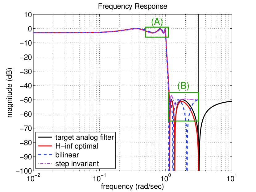
Figure 7: Frequency response of filters: target analog filter $G(s)$ (solid black), sampled-data $H^{\infty}$-optimal $K_{\mathrm{sd}}(z)$ (solid red), bilinear transformation $K_{{\mathrm{bt}},\omega_{0}}(z)$ with frequency prewarping at $\omega_{0}=1$ (rad/sec) (dashed blue), and step-invariant transformation (dash-dotted magenta).

Enlarged plots of the frequency response in passband and stopband are also shown in Fig. 8

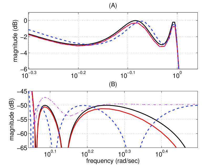
Figure 8: Enlarged plots of Fig. 7 in passband (top) and stopband (bottom).

These plots show that the proposed sampled-data $H^{\infty}$-optimal discretization $K_{\mathrm{sd}}(z)$ shows the best approximation among the filters. The step-invariant transformation $K_{\mathrm{d}}(z)$ is almost the same as $K_{\mathrm{sd}}(z)$ in passband, while its stopband response is quite different from that of the target filter $G(s)$. The bilinear transformation $K_{{\mathrm{bt}},\omega_{0}}(z)$ shows the best performance around the cut-off frequency $\omega_{0}=1$ (rad/sec) at the cost of deterioration of performance at the other frequencies. In summary, the sampled-data $H^{\infty}$ discretization outperforms conventional discretization methods in particular in high-frequency range.

Then we consider an advantage of multirate systems. We compare the sampled-data $H^{\infty}$-optimal multirate system with the single-rate one designed above. We set the upsampling ratio $L=4$. We simulate time response of reconstructing a rectangular input signal $u(t)$ shown in Fig. 9.

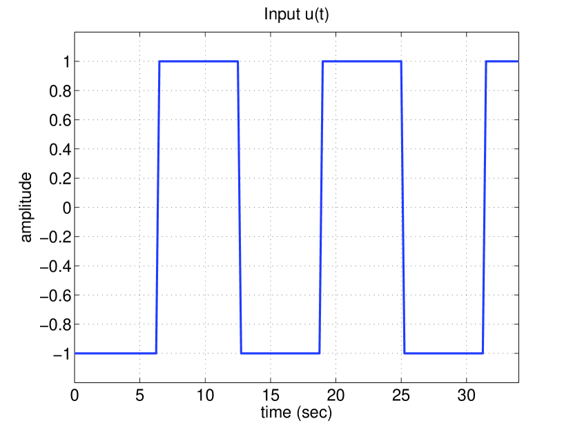
Figure 9: Input signal $u(t)$.

Fig. 10 shows the time response of the single-rate and multirate systems.

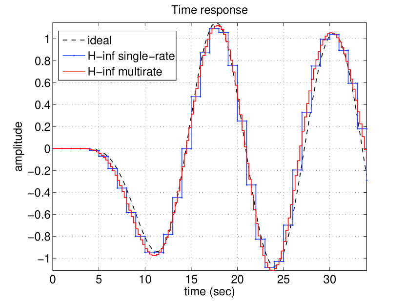
Figure 10: Time response: delayed ideal response $y=(Gu)(\cdot-mh)$ (dashed), response of $H^{\infty}$-optimal single-rate system (blue), and that of $H^{\infty}$-optimal multirate system (red).

The multirate system approximates the ideal response more precisely with a slow-rate samples $\{u(0),u(1),\dots\}$. This is an advantage of the multirate system. In fact, the approximation error becomes smaller when we use larger $L$. To show this, we take upsampling ratio as $L=1,2,4,8,16$, and compute the $H^{\infty}$ norm of the sampled-data error system ${\mathcal{E}}$. Fig. 11 shows the result.

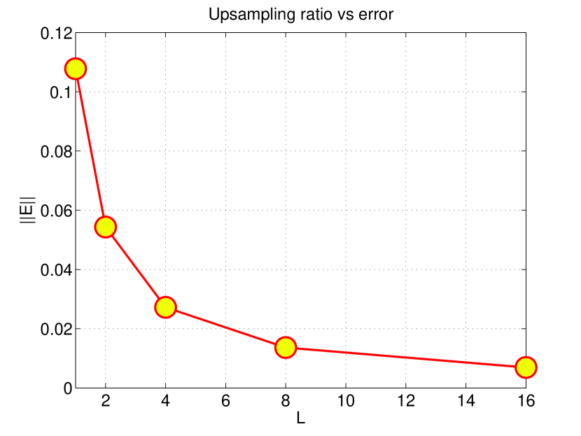
Figure 11: Upsampling ratio $L$ versus approximation error $\|{\mathcal{E}}\|_{\infty}$.

The figure shows the performance gets better when the upsampling ratio is increased.

8 CONCLUSIONS

In this article, we have proposed a discretization method for analog filters via sampled-data $H^{\infty}$ control theory. The design is formulated as a sampled-data $H^{\infty}$ optimization problem, which is approximately reduced to a standard discrete-time $H^{\infty}$ optimization. We have also proposed discretization with multirate systems, which may improve the approximation performance. We have also discussed feedback controller discretization with respect to stability. Design examples show the effectiveness of the proposed method compared with conventional bilinear transformation and step-invariant transformation.

References

- [1] K. J. Åström and T. Hägglund, “The future of PID control,” Control Engineering Practice, vol. 9, no. 11, pp. 1163–1175, 2001.
- [2] T. Chen and B. A. Francis, Optimal Sampled-data Control Systems. Springer, 1995.
- [3] S. Elliott and P. Nelson, “Active noise control,” IEEE Signal Processing Mag., vol. 10, no. 4, pp. 12–35, Oct. 1993.
- [4] J. P. Keller and B. D. O. Anderson, “A new approach to the discretization of continuous-time systems,” IEEE Trans. Automat. Contr., vol. 37, no. 2, pp. 214–223, 1992.
- [5] M. Nagahara, “YY filter — a paradigm of digital signal processing,” in Perspectives in Mathematical System Theory, Control, and Signal Processing. Springer, 2010, pp. 331–340.
- [6] M. Nagahara, “Min-max design of FIR digital filters by semidefinite programming,” in Applications of Digital Signal Processing. InTech, Nov. 2011, pp. 193–210.
- [7] M. Nagahara, M. Ogura, and Y. Yamamoto, “ design of periodically nonuniform interpolation and decimation for non-band-limited signals,” SICE Journal of Control, Measurement, and System Integration, vol. 4, no. 5, pp. 341–348, 2011.
- [8] P. P. Vaidyanathan, Multirate Systems and Filter Banks. Prentice Hall, 1993.
- [9] Y. Yamamoto, B. D. O. Anderson, and M. Nagahara, “Approximating sampled-data systems with applications to digital redesign,” in Proc. 41st IEEE CDC, 2002, pp. 3724–3729.
- [10] Y. Yamamoto, B. D. O. Anderson, M. Nagahara, and Y. Koyanagi, “Optimizing FIR approximation for discrete-time IIR filters,” IEEE Signal Processing Lett., vol. 10, no. 9, pp. 273–276, 2003.
- [11] Y. Yamamoto, A. G. Madievski, and B. D. O. Anderson, “Approximation of frequency response for sampled-data control systems,” Automatica, vol. 35, no. 4, pp. 729–734, 1999.
- [12] Y. Yamamoto, M. Nagahara, and P. P. Khargonekar, “Signal reconstruction via sampled-data control theory — Beyond the shannon paradigm,” IEEE Trans. Signal Processing, vol. 60, no. 2, pp. 613–625, 2012.
- [13] Y. Yamamoto, M. Nagahara, and P. P. Khargonekar, “A brief overview of signal reconstruction via sampled-data optimization,” Applied and Computational Mathematics, vol. 11, no. 1, pp. 3–18, 2012.
- [14] K. Zhou, J. C. Doyle, and K. Glover, Robust and Optimal Control. Prentice Hall, 1996.