$L^{1}$-Optimal Splines for Outlier Rejection

Abstract

In this article, we consider control theoretic splines with $L^{1}$ optimization for rejecting outliers in data. Control theoretic splines are either interpolating or smoothing splines, depending on a cost function with a constraint defined by linear differential equations. Control theoretic splines are effective for Gaussian noise in data since the estimation is based on $L^{2}$ optimization. However, in practice, there may be outliers in data, which may occur with vanishingly small probability under the Gaussian assumption of noise, to which $L^{2}$-optimized spline regression may be very sensitive. To achieve robustness against outliers, we propose to use $L^{1}$ optimality, which is also used in support vector regression. A numerical example shows the effectiveness of the proposed method.

Keywords: control theoretic splines, smoothing, $L^{1}$ optimization, outlier rejection, support vector regression, convex optimization

1 Introduction

Control theoretic spline is generalization of the smoothing spline proposed in Kimeldorf & Wahba (1971), Wahba (1990), using control theoretic ideas, by which the spline curve is determined by the output of a linear control system. Control theoretic splines give a richer class of smoothing curves relative to polynomial curves. They have been proved to be useful for trajectory planning in Egerstedt & Martin (2001), mobile robots in Takahashi & Martin (2004), contour modeling of images in Kano et al. (2008), probability distribution estimation in Charles et al. (2010), to name a few. For more applications and a rather complete theory of control theoretic splines, see Egerstedt & Martin (2010).

Control theoretic splines are effective for reducing Gaussian noise in data since the estimation is based on $L^{2}$ optimization. This means that the noise distribution is assumed to decay very rapidly as the amplitude increases ($\propto e^{-|x|^{2}/2}$). However, in practice, there may exist outliers in data, which may occur with vanishingly small probability under the assumption of the Gaussian distribution of noise. To such noise, $L^{2}$-optimized spline regression may be very sensitive.

Instead, we adopt $L^{1}$ optimality for regression to achieve robustness against outliers. That is, we assume Laplacian distribution for noise, which is distributed much more slowly ($\propto e^{-|x|}$) than Gaussian tails. This is related to support vector regression (SVR) (see e.g. Schölkopf & Smola (2002)), which can be reduced to convex optimization that can be efficiently solved by numerical optimization (see e.g. Boyd & Vandenberghe (2004)).

2 $L^{1}$-Optimal Splines

Consider the following linear system $P$:

$$P:\left\{\begin{split}\dot{{\boldsymbol{x}}}(t)&=A{\boldsymbol{x}}(t)+{\boldsymbol{b}}u(t),&\\ y(t)&={\boldsymbol{c}}^{\top}{\boldsymbol{x}}(t),&t\in[0,\infty).\end{split}\right.$$ (1)

where $A\in{\mathbb{R}}^{n\times n}$, ${\boldsymbol{b}},{\boldsymbol{c}}\in{\mathbb{R}}^{n}$, ${\boldsymbol{x}}(0)={\boldsymbol{0}}\in{\mathbb{R}}^{n}$. We assume $(A,{\boldsymbol{b}})$ is controllable and $({\boldsymbol{c}}^{\top},A)$ is observable. For this system, suppose that we are given data $\mathcal{D}:=\{(t_{1},y_{1}),(t_{2},y_{1}),\ldots(t_{N},y_{N})\}$, where $t_{1},\ldots,t_{N}$ are sampling instants which satisfy $0<t_{1}<t_{2}<\cdots<t_{N}=:T$. The objective here is to find the control input $u(t)$, $t\in[0,T]$ for the system (1) such that $y(t_{i})\approx y_{i}$ for $i=1,\ldots,N$. For this purpose, the following quadratic cost function has been introduced in Sun et al. (2000), Egerstedt & Martin (2010):

$$J_{\mathrm{q}}(u):=\lambda\int_{0}^{T}|u(t)|^{2}{\mathrm{d}}t+\sum_{i=1}^{N}w_{i}(y(t_{i})-y_{i})^{2},$$ (2)

where $\lambda>0$ is the regularization parameter that specifies the tradeoff between the smoothness of $u$ defined in the first term of (2) and the minimization of the empirical risk in the second term. Also, $w_{i}>0$ is a weight for $i$-th empirical risk. The optimal control $u=u_{\mathrm{q}}^{\ast}$ that minimizes $J_{\mathrm{q}}(u)$ is given by Sun et al. (2000), Egerstedt & Martin (2010) as

$$u_{\mathrm{q}}^{\ast}(t)=\sum_{i=1}^{N}\theta_{{\mathrm{q}}}^{\ast}[i]g_{i}(t),$$ (3)

where $g_{i}(t)$ is defined by

$$g_{i}(t):=\begin{cases}{\boldsymbol{c}}^{\top}e^{A(t_{i}-t)}{\boldsymbol{b}},&\quad\text{if}~{}~{}t_{i}>t,\\ 0,&\quad\text{if}~{}~{}t_{i}\leq t,\end{cases}$$ (4)

and the optimal coefficients $\theta_{\mathrm{q}}[1],\dots,\theta_{\mathrm{q}}[N]$ are given by given by

$${\boldsymbol{\theta}}_{\mathrm{q}}^{\ast}:=\bigl{[}\theta_{{\mathrm{q}}}^{\ast}[1],\ldots,\theta_{{\mathrm{q}}}^{\ast}[N]\bigr{]}^{\top}=(\lambda W^{-1}+G)^{-1}{\boldsymbol{y}},$$ (5)

where ${\boldsymbol{y}}:=[y_{1},\ldots,y_{N}]^{\top}$. The matrix $G$ in (5) is the Grammian defined by $G_{ij}=\langle g_{i},g_{j}\rangle$, $i,j=1,\ldots,N$.

In (2), the empirical risk (the second term) is measured by $L^{2}$ norm. This is based on the assumption that the noise added to the data is Gaussian. However, there may exist outliers in data, which may be ignored under the Gaussian assumption of noise. To such outliers, the regression may be very sensitive.

To overcome this, we introduce the following distribution function instead of Gaussian, called $\epsilon$-insensitive function (see Schölkopf & Smola (2002)):

$$p(\xi)=\frac{1}{2(1+\epsilon)}\exp(-|\xi|_{\epsilon}),$$ (6)

where $\epsilon>0$ is a fixed parameter and $|\xi|_{\epsilon}:=\max(|\xi|-\epsilon,0)$. The distribution is an ”insensitive” version of the Laplace distribution, which is given by setting $\epsilon=0$.

The distribution (6) has heavier tails than the Gaussian distribution, and hence leads to more robust regression against outliers. Assuming this distribution, we introduce the following cost function:

$$J:=\frac{1}{2}\|{\boldsymbol{\theta}}\|_{2}^{2}+C\sum_{i=1}^{N}\bigl{|}{\boldsymbol{\theta}}^{\top}{\boldsymbol{\varphi}}_{i}-y_{i}\bigr{|}_{\epsilon},$$ (7)

where $C>0$ is the regularization parameter and ${\boldsymbol{\varphi}}_{i}:=\left[G_{i1},G_{i2},\ldots,G_{iN}\right]^{\top}$.

The optimization above can be effectively solved by employing the method of support vector regression (see Schölkopf & Smola (2002)). That is, the optimization is reduced to the following convex optimization:

$$\begin{split}\text{minimize}~{}~{}&\frac{1}{2}\|{\boldsymbol{\theta}}\|_{2}^{2}+C\sum_{i=1}^{N}\left(\xi_{i}+\hat{\xi}_{i}\right)\\ \text{subject to}~{}~{}&y_{i}\leq{\boldsymbol{\theta}}^{\top}{\boldsymbol{\varphi}}_{i}+\epsilon+\xi_{i},~{}y_{i}\geq{\boldsymbol{\theta}}^{\top}{\boldsymbol{\varphi}}_{i}-\epsilon-\hat{\xi}_{i},~{}\xi_{i}\geq 0,~{}\hat{\xi}_{i}\geq 0.\end{split}$$

3 Example

We here show an example. Let us consider a linear system (1) with

$$A=\begin{bmatrix}0&1\\ 1&0\end{bmatrix},\quad{\boldsymbol{b}}=\begin{bmatrix}1\\ 0\end{bmatrix},\quad{\boldsymbol{c}}^{\top}=\begin{bmatrix}0&1\end{bmatrix}.$$

Note that this system has its transfer function as $P(s)=\frac{1}{(s+1)(s-1)}$. The sampling instants are taken by $t_{i}=0.1+(i-1)\times 0.25$, $i=1,2,\ldots,21$, and the data $y_{i}$ is generated by $y_{i}=\sin 2t_{i}+e_{i}$, where $e_{1},\ldots,e_{21}$ are noise and including an outlier at $t_{7}=1.6$ as shown in Fig. 1.

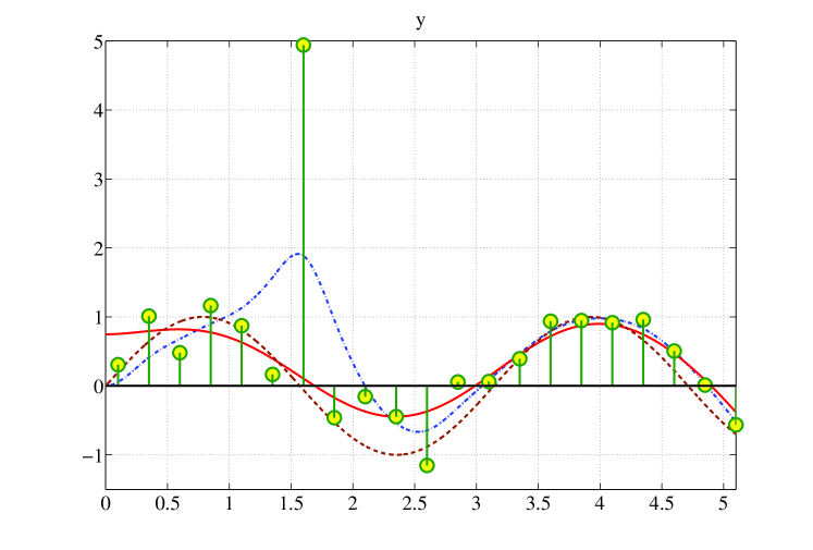
Figure 1: Original curve $y(t)=\sin 2t$ (dashed line), sampled data $\mathcal{D}$ (circles), reconstructed curves via $L^{1}$ optimization (solid line) and via $L^{2}$ optimization (dash-dotted line).

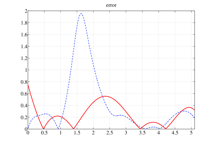
Figure 2: Regression error via $L^{1}$ optimization (solid line) and via $L^{2}$ optimization (dash-dotted line).

With these data, we compute two kinds of control; the proposed control $u^{\ast}$ with ${\boldsymbol{\theta}}={\boldsymbol{\theta}}^{\ast}$ minimizing $J$ in (7), and the conventional $L^{2}$-optimal control $u_{\mathrm{q}}^{\ast}$ minimizing $J_{\mathrm{q}}$ in (2). The regression result is shown in Fig. 1. Fig. 2 also shows the regression error. We can see that the conventional $L^{2}$-optimal regression shows high sensitivity to the outlier and around there the regression error becomes very large. On the other hand, the result by the proposed $L^{1}$ optimization shows much more robust regression.

4 Conclusion

In this article, we have proposed outlier rejection for control theoretic splines based on $L^{1}$ optimization. While conventional $L^{2}$-based splines are effective for Gaussian noise, they are very sensitive to outliers. To achieve robustness against them, we have propose to adopt $L^{1}$ optimality in the regression. A numerical example has shown the effectiveness of our method. Future works include to design constrained splines as discussed in Nagahara & Martin (2013), and to investigate the sparsity property of $L^{1}$-optimal splines as in Nagahara & Quevedo (2011), Nagahara, Matsuda & Hayashi (2012), Nagahara, Quevedo & Østergaard (2012).

References

- (1)
- Boyd & Vandenberghe (2004) Boyd, S. & Vandenberghe, L. (2004), Convex Optimization, Cambridge University Press.
- Charles et al. (2010) Charles, J. K., Sun, S. & Martin, C. F. (2010), Cumulative distribution estimation via control theoretic smoothing splines, in ‘Three Decades of Progress in Control Sciences’, Springer, pp. 83–92.
- Egerstedt & Martin (2010) Egerstedt, M. & Martin, C. (2010), Control Theoretic Splines, Princeton University Press.
- Egerstedt & Martin (2001) Egerstedt, M. & Martin, C. F. (2001), ‘Optimal trajectory planning and smoothing splines’, Automatica 37(7), 1057–1064.
- Kano et al. (2008) Kano, H., Egerstedt, M., Fujioka, H., Takahashi, S. & Martin, C. F. (2008), ‘Periodic smoothing splines’, Automatica 44(1), 185–192.
- Kimeldorf & Wahba (1971) Kimeldorf, G. & Wahba, G. (1971), ‘Some results on Tchebycheffian spline functions’, Journal Math. Anal. Appl. 33(1), 82–95.
- Nagahara & Martin (2013) Nagahara, M. & Martin, C. F. (2013), ‘Monotone smoothing splines using general linear systems’, Asian Journal of Control 5(2), 461–468.
- Nagahara, Matsuda & Hayashi (2012) Nagahara, M., Matsuda, T. & Hayashi, K. (2012), ‘Compressive sampling for remote control systems’, EICE Trans. on Fundamentals E95-A(4), 713–722.
- Nagahara & Quevedo (2011) Nagahara, M. & Quevedo, D. E. (2011), Sparse representations for packetized predictive networked control, in ‘Proc. of IFAC 18th World Congress’, pp. 84–89.
- Nagahara, Quevedo & Østergaard (2012) Nagahara, M., Quevedo, D. E. & Østergaard, J. (2012), Packetized predictive control for rate-limited networks via sparse representation, in ‘Proc. of 51th IEEE CDC’, pp. 1362–1367.
- Schölkopf & Smola (2002) Schölkopf, B. & Smola, A. J. (2002), Learning with Kernels, MIT Press.
- Sun et al. (2000) Sun, S., Egerstedt, M. B. & Martin, C. F. (2000), ‘Control theoretic smoothing splines’, IEEE Trans. on Automatic Control 45(12), 2271–2279.
- Takahashi & Martin (2004) Takahashi, S. & Martin, C. F. (2004), Optimal control theoretic splines and its application to mobile robot, in ‘Proc. of the 2004 IEEE CCA’, pp. 1729–1732.
- Wahba (1990) Wahba, G. (1990), Spline Models for Observational Data, SIAM.