Field Theory of the $d+t\to n+\alpha$ Reaction
Dominated by a ${}^{5}{\rm He}^{*}$ Unstable Particle

Abstract

An effective, non-relativistic field theory for low-energy $dt\leftrightarrow n\alpha$ reaction is presented. The theory assumes that the reaction is dominated by an intermediate ${}^{5}{\rm He}^{*}$ unstable spin $3/2^{+}$ resonance. It involves two parameters in the coupling of the $dt$ and $n\alpha$ particles to the unstable resonant state, and the resonance energy level — only three real parameters in all. All Coulomb corrections to this process are computed. The resultant field theory is exactly solvable and provides an excellent description of the $dt$ fusion process.

I Introduction and Summary

I.0.1 Motivation, Purpose

In this paper, we examine the reaction

$$d+t\leftrightarrow n+\alpha\,.$$ (1)

from an effective field theory point of view. We employ modern techniques of many-body, non-relativistic quantum field theory to describe this reaction, and also make use of the contemporary ideas of effective field theory. In the modern effective field theory approach, stable nuclei (which are treated as particles) and resonant nuclear states (which are treated as unstable particles) are described by individual fields. The fields that correspond to asymptotic states produce particles when they act on the vacuum (no-particle) state. But fields that correspond to resonances have no corresponding single-particle states. For the reaction that we consider in this paper, we shall assume that only a single intermediate resonant state, corresponding to a spin ${3/2}^{+}$ ${{}^{5}{\rm He}}^{*}$, is needed. Thus we shall have creation and annihilation fields for this unstable intermediate resonance as well as such fields for deuteron, triton, alpha, and neutron particles.

The effective field theory is a generalization of the pseudo-potential method introduced by Fermi Fermi in 1936 for low-energy neutron scattering on molecules. Fermi used a $\delta({\bf r})$ function potential taken in first Born approximation. The constant multiplying the $\delta$ function was chosen to give the correct scattering length on a nucleus. The use of a field to describe a composite nucleus was done as early as 1973 by Schwinger Julian when he described the deuteron and used this description to re-derive the effective range formula for the deuteron’s form factor and for its photo-disintegration cross section. The modern use of field theory methods in nuclear physics was advocated by Weinberg Steve in 1990.

The effective field theory may be viewed as the simplest mathematical method to implement a “black box” description of nuclear reactions at low energies. This is a theoretical description that uses the fewest number of parameters. If the process involves a resonant intermediate state, then an unstable field is needed in addition to the fields that describe the propagation of the initial and final particles. As the energy of the reacting particles is increased, additional parameters must be included that correspond to coupling constants for field interactions involving spatial gradients, which correspond to interactions that give higher momentum dependence in the reaction amplitudes. The number of parameters required increases rapidly with increasing energy.

Here we are concerned with reactions in the low-energy limit, but with a resonant intermediate state, the ${}^{5}{\rm He}^{*}$ state. This introduces three parameters: two constants $g_{dt}$ and $g_{n\alpha}$ for the coupling of the $dt$ and $n\alpha$ fields to the unstable ${}^{5}{\rm He}^{*}$ field, and the resonant energy of this unstable field.

A traditional method to compute coupled channel nuclear reactions is to use $R$-matrix theory. This theory entails nuclear channel radii as well as excited state energies and channel couplings. The subsequent companion paperBHP describes the one-level $R$-matrix theory for the two $dt$ and $n\alpha$ channels. This paper explains in detail how the zero channel radii limit of this $R$-matrix theory is precisely the result (I.0.2) below for the effective field theory with the coupling to the unstable ${}^{5}{\rm He}^{*}$ particle.

There are several motivations for this work. It provides a detailed example of how effective field theory methods work for a non-trivial example that involves a higher spin unstable field. Coulomb corrections appear not only in the initial state, but also in the unstable field’s self energy involving the $dt$ loop. Field theory methods of angular momentum coupling simplify the computation. The result provides a very accurate description of the $dt$ fusion reaction that involves only three real parameters. Our simple description may be employed in calculations of plasma screening effects that employ field theory methods and thus requires a field theory of the fusion process screen . (This was the initial motivation for our work on this theory.)

I.0.2 Results

Figure 1: Dimensionless version of the astrophysical factor $\overline{S}_{dt\to n\alpha}$ determined by the definition (11) for the $dt$ reaction compared with the experimental data as a function of the deuteron center-of-mass energy $E$. The solid (blue) curve is the best fit of the simple effective field theory result (I.0.2). It has a $\chi^{2}$ per degree of freedom of 0.784. The dashed (red) curve is based on the cross section of Bosch and Hale B&H92 . The multilevel, multichannel $R$-matrix analysis of the ${}^{5}{\rm He}$ system on which the Bosch and Hale cross sections are based includes data for $n\alpha$ and $dt$ elastic scattering, in addition to those for the associated inelastic reactions, at energies equivalent to a laboratory deuteron energy up to 11 MeV. It fits the 2665 experimental data points included using 117 free parameters with a $\chi^{2}$ per degree of freedom of 1.56. The (magenta) squares are the data of Arnold et al. Arn54 ; the (olive) diamonds are the data of Jarmie et al. Jar84 renormalized by a factor of 1.017; the (green) triangles are the relative data of Brown et al. Brn87 renormalized by a factor of 1.025. The necessity of these renormalizations of the experimental data is discussed in the text. The (blue) circles are the older data of Argo et al. Arg52 which we show for completeness but which we do not use in our fit.

Since the paper contains lengthy calculations, it is worthwhile to present the $dt$ fusion result here before plunging into all the details, including Coulomb corrections. A major effect of these is provided by the familiar Gamow barrier penetration factor for the initial charged deuteron and triton particles. It is the square of the Coulomb wave function evaluated a zero particle separation, $\psi^{(C)}_{{\bf p}_{dt}}(0)$,

$$\left|\psi^{(C)}_{{\bf p}_{dt}}(0)\right|^{2}=\frac{2\pi\eta\,}{\exp\{2\pi\eta\}-1}\,,$$ (2)

in which for the deuteron and triton, each with a single electron charge $e$, in ordinary cgs units (but with the $\hbar=1$ convention that we usually follow),

$$\eta=\frac{e^{2}}{v_{dt}}\,,$$ (3)

where $v_{dt}$ is the relative velocity of the deuteron and triton. We use $m_{ab}$ to denote the reduced mass of a pair of particles $a,b$. So the $dt$ momentum in the center-of-mass system is $p_{dt}=m_{dt}\,v_{dt}$, with the energy of this relative motion in the center-of-mass system given by

$$E=\frac{1}{2}m_{dt}\,v_{dt}^{2}=\frac{{\bf p}_{dt}^{2}}{2m_{dt}}\,.$$ (4)

With our convention for the zero point of the energy $W$ in the center-of-mass system,

$$\frac{{\bf p}_{dt}^{2}}{2m_{dt}}=W+\epsilon_{d}+\epsilon_{t}\,,$$ (5)

in which $\epsilon_{d}$ and $\epsilon_{t}$ are the deuteron and triton binding energies. Thus, at a $dt$ threshold where the $dt$ relative momentum vanishes, $W=-\epsilon_{d}-\epsilon_{t}<0$. In our approximation in which the particles interact only with an unstable intermediate field, in addition to this ‘external propagation barrier penetration’, the only other Coulomb corrections are to the $dt$ “bubble graphs” that appear in the unstable ${}^{5}{\rm He}^{*}$ propagator. The inclusion of all Coulomb effects is detailed in the work leading to Eq. (109), which reads:

$$\sigma_{dt\to n\alpha} = \frac{8}{9}4\pi m_{n\alpha}\frac{p_{n\alpha}^{5}}{v_{dt}}\frac{g^{2}_{dt}}{4\pi}\,\frac{g^{2}_{n\alpha}}{4\pi}\left|\psi^{(C)}_{{\bf p}_{dt}}(0)\right|^{2}\left|G_{*}^{(C)}(W)\right|^{2}.$$

Here $p_{n\alpha}$ is the relative momentum in the center-of-mass frame of the produced $n,\alpha$ particles. By energy conservation, it is given by

$$\frac{p_{n\alpha}^{2}}{2m_{n\alpha}}=\frac{p_{dt}^{2}}{2m_{dt}}+Q\,,$$ (7)

were $Q\simeq 17.59$ MeV is the energy release of the reaction. Since the $n\alpha$ pair is produced in a $D$ wave, the amplitude contains a factor of $p_{n\alpha}^{2}$ and the squared amplitude $p_{n\alpha}^{4}$. Phase space of the produced particles gives an additional factor of $p_{n\alpha}$, so that an overall factor of $p_{n\alpha}^{5}$ appears. The couplings of the initial $d,t$ fields and the final $n,\alpha$ fields to the unstable ${}^{5}{\rm He}^{*}$ field are denoted by $g_{dt}$ and $g_{n\alpha}$.

The unstable interacting Green’s function that appears in the fusion cross section is given by

$$\left|G_{*}^{(C)}(W)\right|^{-2}=\Bigg{[}\frac{p_{dt}^{2}}{2m_{dt}}-E_{*}-\frac{g_{dt}^{2}}{4\pi}\,\Delta(W)\Bigg{]}^{2}$$

$$+\Bigg{[}\frac{g_{dt}^{2}}{4\pi}\,2\,m_{dt}\,p_{dt}\,\left|\psi^{(C)}_{p_{dt}}(0)\right|^{2}+\frac{g_{n\alpha}^{2}}{4\pi}\,\frac{2}{3}\,m_{n\alpha}\,p_{n\alpha}^{5}\Bigg{]}^{2}.$$ (8)

This is the function given in Eq. (IV) whose derivation and description precedes Eq. (IV). The energy $E_{*}$ along with the coupling parameters $g_{dt}^{2}$ and $g_{n\alpha}^{2}$ are determined by fitting the $dt\to n\alpha$ fusion cross section.

The function $\Delta$ is a Coulomb-modified $dt$ loop function that is given by [see Eq. (123)]

$$\Delta(W) = \frac{4m_{dt}}{b_{0}}\,\left[{\rm Re}\,\psi(i\eta)-\ln\eta\right]\,,$$ (9)

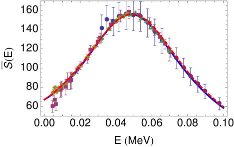
where $b_{0}=1/e^{2}\,m_{dt}=24.04\,{\rm fm}$ and $\psi(z)=\Gamma^{\prime}(z)/\Gamma(z)$ is the logarithmic derivative of the Gamma function. Although the peak in the fusion cross section, or the maximum of the modified astrophysical factor $\overline{S}_{dt\to n\alpha}$ shown in Fig. 1, are determined by $E_{*}$, the positions of these are not directly related to the value of $E_{*}$ since there are shifts brought about by the Coulomb self-energy correction $\Delta(W)$ and by the variation of the factors that involve $p_{dt}$ and $p_{n\alpha}$.

The astrophysical ‘$S$ factor’ is conventionally defined by

$$S=E\,e^{2\pi\eta}\,\sigma\,.$$ (10)

The multiplication by $E=mv^{2}/2$ removes the two factors of $1/v$ that naturally appear in the cross section: the $1/v$ arising from the division of the reaction rate by the incident flux, and the $1/v$ factor that appears in the overall $\eta$ factor in the squared Coulomb wave function (2). The factor $\exp\{2\pi\eta\}$ removes the major exponential factor (the factor which appears in the Gamow barrier penetration approximation) in the squared Coulomb wave function (2). We prefer, however, to use a slightly modified astrophysical ‘$\overline{S}$ factor’ that we define by

$$\overline{S}_{dt\to n\alpha} = \frac{p_{dt}^{2}}{\hbar^{2}}\,\left[e^{2\pi\eta}-1\right]\,\sigma_{dt\to n\alpha}$$ (11)

$$= \frac{2\,m_{dt}}{\hbar^{2}}E\,\left[e^{2\pi\eta}-1\right]\,\sigma_{dt\to n\alpha}\,.$$

Here we have multiplied by $p^{2}$ rather than by $E=p^{2}/2m$ because this makes $\overline{S}$ dimensionless. Moreover, we have multiplied by $[\exp\{2\pi\eta\}-1]$ rather than by only the Gamow barrier penetration factor $\exp\{2\pi\eta\}$ so as to remove the complete energy dependence of the squared Coulomb wave function.

In terms of this notation, our result becomes

$$\overline{S}_{dt\to n\alpha} =\frac{8}{9}\,4\pi\,m_{dt}\,m_{n\alpha}\,p_{n\alpha}^{5}\,\,\frac{g^{2}_{dt}}{4\pi}\,\frac{g^{2}_{n\alpha}}{4\pi}\,\,\frac{2\pi}{b_{0}}\,\,$$

$$\times\left|G_{*}^{(C)}(W)\right|^{2}\,.$$ (12)

A fit of this result to the data reduced to construct $\overline{S}_{dt\to n\alpha}$ is presented in Fig. 1. The fit to the $dt$ fusion cross section with our formula gives the parameter values

$$E_{*} =-154\,\pm 8\,\,{\rm keV}\,,$$

$$\frac{g_{dt}^{2}}{4\pi} =199\,\pm 8\,\,{\rm fm}^{3}\,{\rm MeV}^{2}\,,$$

$$\frac{g_{n\alpha}^{2}}{4\pi} =16.4\,\pm 1.0\,\,{\rm fm}^{7}\,{\rm MeV}^{2}\,.$$ (13)

The early cross-section measurements Arn54 ; Arg52 used to determine the parameters of the fit were reported with rather large uncertainties (typically $\sim 10$%), which combined relative and normalization (scale) uncertainties. However, in the more recent measurement of Jarmie et al. Jar84 , the relative errors were much smaller ($\sim 0.5$%), and were reported separately from the larger scale uncertainty of 1.26%. The subsequent measurement of Brown et al. Brn87 likewise had small relative errors, but no absolute normalization was determined in this experiment. For the purpose of reporting the data, Brown and et al. determined an approximate scale by matching in the region of overlap to the earlier absolute measurement of Jarmie et al..

When fitting these data in the comprehensive ⁵He $R$-matrix analysis that was used to produce the reaction cross sections of Bosch and Hale B&H92 , separate normalization parameters were allowed to vary for each data set, the one for the Jarmie data being constrained in the total $\chi^{2}$ by its 1.26% uncertainty, and the one for the Brown et al. data unconstrained, since it was purely a relative measurement. The values of the renormalization factors found from that analysis, 1.017 for Jarmie et al. Jar84 , and 1.025 for Brown et al. Brn87 , were applied to the experimental data sets (cross sections and uncertainties) prior to performing the more limited fitting of effective field theory result $\bar{S}_{dt\rightarrow n\alpha}$ [Eq. (I.0.2)] over the resonance described here.

Our result, which entails only three parameters, fits the data very well. To achieve this, it is necessary to start with a free-particle Lagrangian for the unstable ${}^{5}{\rm He}^{*}$ field with the “wrong” sign. This would not be acceptable if the theory were taken to be more fundamental with an extended region of validity rather than a effective theory whose applicability is only to the low-energy regime. It is easy to show that the simple theory with two initial spin zero particles which interact via an intermediate (“s-channel”) field (the simple scalar-particle analog of our theory) produces an effective range formula with a negative effective range parameter BHP . A positive effective range parameter is achieved in this theory if the intermediate field has a wrong-sign free-particle Lagrangian. Thus the restricted validity of this simple effective field theory should be acceptable just as is that of the effective range theory.

I.0.3 Outline

Section II.1 explains our conventions for the fields and their free-particle Lagrange functions. Section II.2 defines the interaction Lagrange functions for the coupling of the initial $dt$ and the final $n\alpha$ to the unstable ${}^{5}{\rm He}^{*}$ field and the appropriate spin-orbit combination of the $n\alpha$ fields that enter into their interaction.

Section III describes the dynamics of our theory in the absence of the Coulomb interactions. This is done in some detail because this underlying theory, which involves higher spin fields, has some complexity, and it clarifies the development to proceed with simpler stages. Section III.1 presents the calculation of the self-energy functions for the unstable ${}^{5}{\rm He}^{*}$ propagator using dimensional continuation to define their needed regularization and express the intermediate expressions in term of quantum-mechanical transformation functions that simplifies the subsequent computation of Coulomb corrections. Section III.2 describes our result for the $dt\to n\alpha$ fusion cross section in the absence of Coulomb interactions.

Section IV displays the Coulomb corrections to the fusion process. The $dt$ particles initially interact at a point, thereby bringing about a factor of the squared Coulomb wave function at the origin $|\psi^{(C)}(0)|^{2}$. The $dt$ piece of the resonant state propagator also has Coulomb corrections. Using the formalism developed in Sec. III.1, these corrections become expressed in a dispersion relation form that is a representation of the logarithmic derivative of the Gamma function $\psi(z)$.

After a brief summary of our work in the concluding Section V, unsuccessful approaches to avoid the introduction of the wrong-sign ${}^{5}{\rm He}^{*}$ free propagator are mentioned. We then note how extensions of the effective field theory method to multichannel descriptions of light nuclear reactions might be obtained without great effort.

Appendix A contains a short account of Galilean invariance that provides results needed in the text. Efficient quantum field theory methods that couple spins are explained in Appendix B. The theory of Coulomb corrections is discussed in Appendix C.

II Effective Field Theory: Ingredients

II.1 Fields, Kinematics

As discussed in the Introduction, each particle in our reaction system is described by creation and annihilation fields. The free-field part of the Lagrange function for each of these fields has the generic form

$${\cal L}^{(0)}_{\rm\scriptscriptstyle A}=\chi^{\dagger}_{\rm\scriptscriptstyle A}\,i\,\frac{\partial}{\partial t}\,\chi_{\rm\scriptscriptstyle A}-{\cal H}^{(0)}_{\rm\scriptscriptstyle A}\,,$$ (14)

with

$${\cal H}^{(0)}_{\rm\scriptscriptstyle A}=\chi^{\dagger}_{\rm\scriptscriptstyle A}\left[\frac{-\nabla^{2}}{2m_{\rm\scriptscriptstyle A}}-\epsilon_{\rm\scriptscriptstyle A}\right]\chi_{\rm\scriptscriptstyle A}\,.$$ (15)

As shown in Appendix A, Galilean invariance requires that the inertial mass $m_{\rm\scriptscriptstyle A}$ of a composite nucleus is the sum of the

Particle	Spin	Operators	Mass	Binding
Alpha	$0^{+}$	$\phi^{\dagger}_{\alpha}({\bf r},t),\ \phi_{\alpha}({\bf r},t)$	$m_{\alpha}=2m_{p}+2m_{n}$	$\epsilon_{\alpha}$
Deuteron	$1^{+}$	${\bm{\phi}}_{d}^{\dagger}({\bf r},t),\ \bm{\phi}_{d}({\bf r},t)$	$m_{d}=m_{p}+m_{n}$	$\epsilon_{d}$

Table 1: Bosonic fields and their properties.

Particle	Spin	Operators	Mass	Binding
Neutron	$\tfrac{1}{2}^{+}$	$\psi_{n}^{\dagger}({\bf r},t)$, $\psi_{n}({\bf r},t)$	$m_{n}$	$\epsilon_{n}\equiv 0$
Triton	$\tfrac{1}{2}^{+}$	$\psi_{t}^{\dagger}({\bf r},t)$, $\psi_{t}({\bf r},t)$	$m_{t}=m_{p}+2m_{n}$	$\epsilon_{t}$
5He∗	$\tfrac{3}{2}^{+}$	$\psi_{*}^{\dagger}({\bf r},t)$, $\psi_{*}({\bf r},t)$	$m_{*}=2m_{p}+3m_{n}$	$\epsilon_{*}$

Table 2: Fermionic fields and their properties.

masses of the neutrons and protons of which it is composed. We have written $\epsilon_{\rm\scriptscriptstyle A}>0$ for the binding energy of the composite particle ${\rm\scriptscriptstyle A}$. The total free particle Hamiltonian,

$$H^{(0)}={\sum}_{\rm\scriptscriptstyle A}\,\int(d^{3}{\bf r})\,{\cal H}^{(0)}_{\rm\scriptscriptstyle A}\,,$$ (16)

measures the energy of an asymptotic state where all the particles a separated by large distances.

In view of the structure of the total Hamiltonian (16) with the pieces (15), the total energy $E_{ab}$ of a pair $a\,,\,b$ of stable particles separated by large distances is

$$E_{ab}=\frac{{\bf p}_{a}^{2}}{2m_{a}}-\epsilon_{a}+\frac{{\bf p}_{b}^{2}}{2m_{b}}-\epsilon_{b}=\frac{{\bf P}_{ba}^{2}}{2M_{ab}}+\frac{{\bf p}_{ba}^{2}}{2m_{ab}}-\epsilon_{a}-\epsilon_{b}\,,$$ (17)

in which $M_{ab}$ and $m_{ab}$ are the total and reduced masses of the $a\,,\,b$ system; ${\bf P}_{ba}$ and ${\bf p}_{ba}$ are the total and relative momenta. The energy $W_{ab}$ in the center-of-mass system is the Galilean invariant

$$W_{ab}=E_{ab}-\frac{{\bf P}_{ba}^{2}}{2M_{ab}}=\frac{{\bf p}_{ba}^{2}}{2m_{ab}}-\epsilon_{a}-\epsilon_{b}\,.$$ (18)

Our description of the $d\,t\to n\,\alpha$ reaction will employ only the initial and final particles, the deuteron ($d$), neutron ($n$), and the triton ($t$) alpha ($\alpha$), and a single unstable ⁵He^∗ nucleus. The corresponding bosonic fields and their properties: spin-parity, masses, and binding energies, are listed in Table 1. Note that we conveniently describe the deuteron spin states as a vector representing “linear polarization”; the usual ${J_{z}}^{\prime}=m=\{\pm 1,0\}$ states are the $\{(x\pm iy)/\sqrt{2},z\}$, components of this vector. Properties of the fermionic fields are given in Table 2.

As explained in Appendix B, the condition that the unstable ${}^{5}{\rm He}^{*}$ field carry only spin $3/2$ (with no additional spin $1/2$ piece) can be conveyed in the requirement that this vector-spinor field obeys

$$\bm{\sigma}\cdot\bm{\psi}_{*}({\bf r},t)=0=\bm{\psi}_{*}^{\dagger}({\bf r},t)\cdot\bm{\sigma}\,,$$ (19)

in which $\bm{\sigma}$ are the Pauli spin matrices.

The unstable, resonant ${}^{5}{\rm He}^{*}$ state, has a ‘binding’ energy $\epsilon_{*}$ that is negative so that can decay into a deuteron plus a triton. The conservation of total energy $W$ in the center-of-mass system for the $dt$ fusion reaction gives

$$\frac{{\bf p}_{dt}^{2}}{2m_{dt}}-\epsilon_{d}-\epsilon_{t}=\frac{{\bf p}_{n\alpha}^{2}}{2m_{n\alpha}}-\epsilon_{n}-\epsilon_{\alpha}\,.$$ (20)

At threshold, ${\bf p}_{dt}=0$, and the produced $n,\alpha$ pair has a kinetic energy ${\bf p}^{2}_{n\alpha}/2m_{n\alpha}=Q$. Here $Q$ is the conventional notation for the energy liberated by the reaction. Since by our convention $\epsilon_{n}=0$,

$$Q=\epsilon_{\alpha}-\epsilon_{d}-\epsilon_{t}\simeq 17.59\,\,{\rm MeV}.$$ (21)

II.2 Unstable Particle Interactions

As discussed in the Introduction, the interaction Lagrange function describes the coupling of the reacting particles to an intermediate unstable field that describes a $3/2^{+}$ resonance ⁵He^∗ in the intermediate state:

$${\cal L}_{1} =g_{dt}\left[\bm{\psi}_{*}^{\dagger}\,\,\psi_{t}\cdot\bm{\phi}_{d}+{\bm{\phi}_{d}}^{\,\dagger}\cdot\psi^{\dagger}_{t}\,\bm{\psi}_{*}\right]$$

$$+g_{n\alpha}\left[\bm{\psi}_{*}^{\dagger}\cdot\bm{\Psi}_{\alpha n}+\bm{\Psi}^{\dagger}_{\alpha n}\cdot\bm{\psi}_{*}\right]$$ (22)

Here the $dt$ field pair contains spin $1/2$ as well as spin $3/2$. However, the coupling of this pair to the unstable particle field with spin $3/2$ projects out only the spin $3/2$ part of the $dt$ pair. The coupling of the unstable particle field to the $\alpha n$ pair is more complicated since as discussed in detail in Appendix B, it involves an internal D-wave angular momentum in this pair. This $l=2$ internal angular momentum combines with the spin $1/2$ in the neutron to produce the spin ${3/2}^{+}$ field $\bm{\Psi}_{\alpha\,n}$. As explained in Appendix B, this field is given by

$$\Psi^{l}_{\alpha\,n}({\bf r},t)=\phi_{\alpha}({\bf r},t)\,{\cal T}^{lm}_{\alpha n}\,\sigma^{m}\,\psi_{n}({\bf r},t)\,,$$ (23)

in which a sum over repeated vector or tensor indices is implied, and with

$${\cal T}^{lm}_{\alpha n}={\cal P}^{l}_{\alpha n}{\cal P}^{m}_{\alpha n}-\frac{1}{3}\,\delta^{lm}\,{\cal P}^{k}_{\alpha n}{\cal P}^{k}_{\alpha n}\,,$$ (24)

where

$${\cal P}^{k}_{\alpha n}=\frac{m_{n\alpha}}{m_{n}}\frac{1}{i}\stackrel{{\scriptstyle\rightarrow}}{{\nabla}}^{k}-\frac{m_{n\alpha}}{m_{\alpha}}\frac{1}{i}\stackrel{{\scriptstyle\leftarrow}}{{\nabla}}^{k}\,,$$ (25)

with $m_{n\alpha}$ the reduced mass of the alpha-neutron system. The arrow over a derivative indicates whether the derivative acts to the left or to the right. As we shall see, the differential operator ${\cal P}^{k}_{\alpha n}$ reduces to the relative momenta of the $n\alpha$ pair when the reaction amplitudes are computed.

III Effective Field Theory: Dynamics

The reaction amplitudes may be described by the interaction picture which involves free-field matrix elements of the time-ordered, unitary evolution operator

$$U=\left(\exp\left\{i\int dt\int(d^{3}{\bf r})\,{\cal L}_{1}\right\}\right)_{+}\,.$$ (26)

The propagators of non-relativistic fields are retarded functions in time: particles are created at an earlier time and then destroyed at a later time. Hence, on expanding the interaction picture time evolution operator (26), it is easy to see that the only contributions to a two-body reaction with an interaction of the form of Eq. (II.2) are as follows. Starting at an early time, the initial particle pair is destroyed and the unstable ⁵He^∗ particle is created. In the leading order expansion of the evolution operator, this unstable particle decays into the particles in the final state. In the next-to-leading order, the unstable particle propagates for some time and then decays into a particle pair. Each particle in this pair now propagates for another period of time until the pair is destroyed with the creation of another unstable particle. This chain of “bubbles” goes on until the final two-particle state is reached. The first terms in the expansion of the evolution operator give a single “bubble” surrounded by two unstable free-field propagators. The next set of expansion terms give two “bubbles” joined by three unstable free-field propagators. And so forth to result in an infinite set of graphs consisting of alternating lines and “bubbles”.

We consider in the next subsection, Sec. III.1, the unstable particle Green’s function neglecting the Coulomb interaction. This allows us to focus on the evaluation of the $n\alpha$ and $dt$ contributions to the self-energy, $\Sigma_{n\alpha}(W)$ and $\Sigma_{dt}(W)$. These are sufficiently complex computations, even with the neglect of the instantaneous Coulomb interactions, to warrant a dedicated discussion. Then, in following Sec. IV, we include corrections due to the instantaneous Coulomb interactions for these particles.

Figure 2: Diagrammatic structure of the interacting ⁵He^∗ Green’s function. The thick, directed line represents the interacting Green’s function with all its self-energy corrections. The double line stands for the wrong-sign free-particle propagator. The shaded region immediately to the right of the free propagator represents the $n\alpha$ and $dt$ self-energies contained in the $\Sigma(W)$ that appears in Eq. (30).

Figure 3: The self-energy diagrams of the ⁵He^∗, neglecting the instantaneous Coulomb interaction, corresponding to Eq. (30). Shaded boxes indicate the $g_{n\alpha}$ and $g_{dt}$ vertices appropriate to each graph. The first loop graph on the right-hand side describes the $n\alpha$ contribution Eq. (91); the second loop graph corresponds to the $dt$ contribution Eq. (90).

III.1 Unstable Particle Green’s Function

The unstable particle’s Green’s function may be expressed as

$$G_{*}^{lm}({\bf r}-{\bf r}^{\prime},t-t^{\prime}) =\int\frac{(d^{3}{\bf p})}{(2\pi)^{3}}\frac{dE}{2\pi}\,e^{i{\bf p}\cdot({\bf r}-{\bf r}^{\prime})-iE(t-t^{\prime})}$$

$$\times P_{3/2}^{lm}\,G_{*}(W)\,.$$ (27)

Here $P_{3/2}^{lm}$ is the projection matrix (166) into the spin $3/2$ subspace. It is a matrix in the $2\times 2$ spinor space and a second-rank tensor in the vector indices exhibited. Because of Galilean invariance, the scalar factor $G_{*}(W)$ is a function only of the energy in the center-of-mass frame

$$W=E-\frac{p^{2}}{2m_{*}}\,.$$ (28)

The unstable ${}^{5}{\rm He}^{*}$ inverse Green’s function scalar factor has the form

$$G_{*}^{-1}(W)=-(W+\epsilon_{*})-\Sigma(W+i\eta)\,,$$ (29)

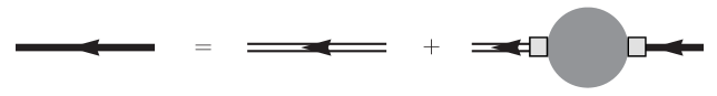
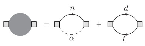
where, as discussed at some length in the Introduction and Summary above, the free-particle piece is taken corresponding to a wrong-sign Lagrangian. The structure of the corresponding Green’s function is described by an integral equation in space-time which reduces to an algebraic equation in momentum-frequency space as indicated by the diagram in Fig. 3. The self-energy $\Sigma(W)$ is the sum of a $dt$ part and an $n\alpha$ part:

$$\Sigma(W)=\Sigma_{dt}(W)+\Sigma_{n\alpha}(W)\,.$$ (30)

The self-energy functions, corresponding to $dt$ and $n\alpha$ loop graphs, is displayed in Fig. 3.

The $dt$ contribution involves the propagator or Green’s function for the spin-one deuteron which has the simple tensor structure $G_{d}^{kl}=\delta^{kl}\,G_{d}$, where $G_{d}$ is a scalar function, and the Green’s function for the triton which is a unit matrix in the $2\times 2$ spinor space times a scalar function $G_{t}$. The unit tensor $\delta^{kl}$ describing the deuteron spin and the unit matrix in the deuteron spin space both act as unity when acting upon the components of the unstable field Green’s function. Hence, the $dt$ loop can be written as the scalar function

$$\Sigma_{dt}(W)=i\,g_{dt}^{2}\,\int(d^{3}\bar{\bf r})\,dt\,e^{-i{\bf p}\cdot\bar{\bf r}+iE\,t}\,G_{d}(\bar{\bf r},t)\,G_{t}(\bar{\bf r},t)\,.$$ (31)

The scalar part of the Green’s functions have the generic form

$$G({\bf r}-{\bf r}^{\prime},t-t^{\prime})=-i\Big{\langle}0\Big{|}\left(\chi({\bf r},t)\chi^{\dagger}({\bf r}^{\prime},t^{\prime})\right)_{+}\Big{|}0\Big{\rangle}$$

$$=-i\theta(t-t^{\prime})\int\frac{(d^{3}{\bf p})}{(2\pi)^{3}}e^{i{\bf p}\cdot({\bf r}-{\bf r}^{\prime})}e^{iE(p)(t-t^{\prime})},$$ (32)

in which $\theta$ is the unit step function and

$$E(p)=\frac{{\bf p}^{2}}{2m}-\epsilon$$ (33)

is the energy which includes the binding energy $-\epsilon$ as well as the kinetic energy with a mass $m$ that is the sum of the nucleon masses that make up the nucleus described by the field $\chi$.

Such Green’s functions have the structure of a time-dependent, quantum-mechanical transformation function of a free particle. It will prove convenient to write them in this form, namely as

$$G({\bf r}-{\bf r}^{\prime},t-t^{\prime})=-i\langle{\bf r},t|{\bf r}^{\prime},t^{\prime}\rangle^{(0)}\,\theta(t-t^{\prime})\,.$$ (34)

Here we have included the superscript to indicate that we are evaluating the free-particle transformation function with no Coulomb interactions. Later in Sec. IV, when we turn to the Coulomb corrections, this superscript will indicate the evaluation of the transformation function in the presence of the Coulomb interaction with $(0)\to(C)$. It is useful to use this relation because it is then natural to pass to center-of-mass and relative coordinates and write

$$G_{b}({\bf r}_{b}-{\bf r}_{b}^{\prime},t-t^{\prime})\,G_{a}({\bf r}_{a}-{\bf r}_{a}^{\prime},t-t^{\prime})$$

$$=-\langle{\bf R},t|{\bf R}^{\prime},t^{\prime}\rangle^{(0)}_{ba\,\,\rm CM}\,\,\langle{\bf r},t|{\bf r}^{\prime},t^{\prime}\rangle^{(0)}_{ba\,\,\rm rel}\,\,\theta(t-t^{\prime})\,.$$ (35)

Here, as usual,

$${\bf R}=\frac{m_{a}{\bf r}_{a}+m_{b}{\bf r}_{b}}{m_{a}+m_{b}}\,,\qquad\qquad{\bf r}={\bf r}_{b}-{\bf r}_{a}$$ (36)

are the center-of-mass and relative coordinates. The free-particle dynamics in the transformation function of the relative motion $\langle{\bf r},t|{\bf r}^{\prime},0\rangle^{(0)}_{ba\,\,\rm rel}$ is described by the Hamiltonian

$$H_{ba\,\,\rm rel}=\frac{{\bf p}_{ba}^{2}}{2m_{ab}}-\epsilon_{b}-\epsilon_{a}$$ (37)

that contains the binding energies displayed in Eq. (33) so as to provide the correct reference energy. We shall find this decomposition helpful when we compute the Coulomb corrections to the reactions. To return to the evaluation of the self-energy function $\Sigma_{dt}$, we note that at the coincident points ${\bf r}_{d}={\bf r}_{t}=\bar{\bf r}$, ${\bf R}=\bar{\bf r}$, and we encounter

$$\int(d^{3}\bar{\bf r})\,e^{-i{\bf p}\cdot\bar{\bf r}}\langle\bar{\bf r},t|{\bf 0},0\rangle^{(0)}_{ba\,\,\rm CM}$$

$$=\exp\left\{-i\frac{{\bf p}^{2}}{2M_{ba}}\,t\right\}\,.$$ (38)

In the present case, $M_{ba}=m_{d}+m_{t}=2m_{p}+3m_{n}=m_{*}$. Hence the self-energy function involves a Fourier transform in time with a single energy variable $W=E-{\bf p}^{2}/2m_{*}$, as must be the case in virtue of the Galilean invariance of the theory, and we have

$$\Sigma_{dt}(W) =-ig_{dt}^{2}\int_{0}^{\infty}dt\,e^{iWt}\langle{\bf 0},t|{\bf 0},0\rangle^{(0)}_{dt\,\,\rm rel}\,.$$ (39)

To evaluate the loop function that appears in the self-energy $\Sigma_{n\alpha}(w)$, we note that it entails

$$\left\langle 0\left|\Psi^{k}_{\alpha\,n}(\bar{\bf r},t)\Psi^{l}_{\alpha\,n}(\bar{\bf r}^{\prime},t)\right|0\right\rangle$$

$$=\left\langle 0\left|\phi_{\alpha}(\bar{\bf r},t)\,{\cal T}^{km}_{\alpha n}\sigma^{m}\psi_{n}(\bar{\bf r},t)\psi_{n}^{\dagger}(\bar{\bf r}^{\prime},t)\sigma^{n}{\cal T}^{nl}_{\alpha n}\phi_{\alpha}^{\dagger}(\bar{\bf r}^{\prime},t)\right|0\right\rangle$$

$$=\langle\bar{\bf r},t|\bar{\bf r}^{\prime},t^{\prime}\rangle^{(0)}_{ba\rm CM}\sigma^{m}\sigma^{n}\left.\left[\nabla^{k}\nabla^{m}-\frac{1}{3}\delta^{km}\nabla^{2}\right]\right.$$

$$\times\left.\left[\nabla^{n}\nabla^{l}-\frac{1}{3}\delta^{nl}\nabla^{2}\right]\langle{\bf r},t|{\bf 0},0\rangle^{(0)}_{ba\rm rel}\right|_{{\bf r}={\bf 0}}.$$ (40)

Here we have made use of the translational invariance of the free-particle transformation function $\langle{\bf r},t|{\bf r}^{\prime},0\rangle^{(0)}_{ba\,\,\rm rel}=\langle{\bf r}-{\bf r}^{\prime},t|{\bf 0},0\rangle^{(0)}_{ba\,\,\rm rel}$ to write all the derivatives on the left as shown. Since the ${\bf r}\to{\bf 0}$ limit yields a rotationally invariant function whose tensor structure can only involve the unit tensor $\delta^{{}^{{\bf..}}}$, we have

$$\left[\nabla^{k}\nabla^{m}-\frac{1}{3}\delta^{km}\nabla^{2}\right]$$

$$\times\left[\nabla^{n}\nabla^{l}-\frac{1}{3}\delta^{nl}\nabla^{2}\right]\langle{\bf r},t|{\bf 0},0\rangle^{(0)}_{ba\rm rel}\Big{|}_{{\bf r}={\bf 0}}.$$

$$=\frac{1}{15}\left[\delta^{kn}\delta^{ml}+\delta^{kl}\delta^{mn}-\frac{2}{3}\delta^{km}\delta^{nl}\right]$$

$$\times\left(\nabla^{2}\right)^{2}\langle{\bf r},t|{\bf 0},0\rangle^{(0)}_{ba\rm rel}\Big{|}_{{\bf r}={\bf 0}},$$ (41)

as contractions with various $\delta^{{}^{{\bf..}}}$ establishes. Placing this result in Eq. (40), using the Pauli matrix composition law (154) and the form (166) of the spin $3/2$ projection matrix, we conclude that

$$\left\langle 0\left|\Psi^{k}_{\alpha\,n}(\bar{\bf r},t)\,\Psi^{l}_{\alpha\,n}({\bf 0},0)\right|0\right\rangle$$

$$=\langle\bar{\bf r},t|{\bf 0},0\rangle^{(0)}_{\alpha n\,\,\rm CM}\,\,\frac{1}{3}\,P^{kl}_{3/2}\,$$

$$\times\left(\nabla^{2}\right)^{2}\,\langle{\bf r},t|{\bf 0},0\rangle^{(0)}_{\alpha n\,\,\rm rel}\Big{|}_{{\bf r}={\bf 0}}\,.$$ (42)

The projection matrix $P^{kl}_{3/2}$ that appears here can be omitted. It either acts upon the ${}^{5}{\rm He}^{*}$ propagator that only contains spin $3/2^{+}$. Hence it can be replaced by unity, and just as in the previous evaluation of the $dt$ self-energy function, we have

$$\Sigma_{n\alpha}(W) =-ig_{n\alpha}^{2}\int_{0}^{\infty}dte^{iWt}$$

$$\times\left(\nabla^{2}\right)^{2}\langle{\bf r},t|{\bf 0},0\rangle^{(0)}_{\alpha n\rm rel}\Big{|}_{{\bf r}={\bf 0}}.$$ (43)

To complete the computation, we need to evaluate expressions that are divergent in three spatial dimensions. These divergences can be removed by ‘subtractions’ — by deleting the divergent pieces and replacing them by appropriate mass and wave function renormalizations. In our case, with the highly divergent $n\alpha$ piece, this subtraction method is a cumbersome method. Moreover, it is not a proper, well-defined mathematical procedure. The proper procedure is to first regulate the theory to make it well defined, and then perform whatever renormalizations that are needed. Any regularization scheme must make the theory unphysical in some sense because if it were not, one could have a well-defined, finite theory, and one should use this new theory rather than that which one started with. One regularization scheme is that of Pauli and Villars. It produces a regularized theory with sectors that have negative probabilities until the renormalizations are made and the regularization removed. Here we shall find it very convenient to use dimensional regularization where the three spatial dimensions are continued to an arbitrary $\nu$ dimensional space, and the limit $\nu\to 3$ is performed only after all computations have been performed.

In $\nu$ spatial dimensions

$$\left\{\begin{array}[]{c}1\\ \left(\nabla^{2}\right)^{2}\end{array}\right\}\left.\langle{\bf r},t|{\bf 0},0\rangle^{(0)}_{ba\,\rm rel}\right|_{{\bf r}={\bf 0}}$$ (46)

$$=e^{i(\epsilon_{b}+\epsilon_{a})\,t}\int\frac{(d^{\nu}{\bf p})}{(2\pi)^{\nu}}\left\{\begin{array}[]{c}1\\ \left({\bf p}^{2}\right)^{2}\end{array}\right\}\exp\left\{-it\,\frac{{\bf p}^{2}}{2m_{ba}}\right\}$$ (49)

$$=e^{i(\epsilon_{b}+\epsilon_{a})\,t}\frac{\Omega_{\nu-1}}{(2\pi)^{\nu}}\int_{0}^{\infty}p^{\nu-1}dp\left\{\begin{array}[]{c}1\\ p^{4}\end{array}\right\}\exp\left\{\!-it\frac{p^{2}}{2m_{ba}}\right\}\!,$$ (52)

(53)

where in the second line we have passed to hyper-spherical coordinates with $\Omega_{\nu-1}$ the area of a unit $\nu-1$ sphere embedded in a $\nu$-dimensional space. We change variables, writing explicitly $i=\exp\{\pi i/2\}$ so as to be able to carefully keep track of the phase, to get

$$\left\{\begin{array}[]{c}1\\ \left(\nabla^{2}\right)^{2}\end{array}\right\}\left.\langle{\bf r},t|{\bf 0},0\rangle^{(0)}_{ba\,\,\rm rel}\right|_{{\bf r}={\bf 0}}$$ (56)

$$\qquad\qquad=e^{i\,(\epsilon_{b}+\epsilon_{a})\,t}\,\,\frac{\Omega_{\nu-1}}{(2\pi)^{\nu}}\,\left(\frac{2m_{ba}}{t}\right)^{\nu/2}\,e^{-\nu\pi i/4}\,\frac{1}{2}\,\int_{0}^{\infty}u^{\nu/2}\,\frac{du}{u}\,\left\{\begin{array}[]{c}1\\ -\left(2m_{ba}/t\right)^{2}\,u^{2}\end{array}\right\}\,e^{-u}$$ (59)

$$\qquad\qquad=e^{i\,(\epsilon_{b}+\epsilon_{a})\,t}\,\,\frac{\Omega_{\nu-1}}{(2\pi)^{\nu}}\,\left(\frac{2m_{ba}}{t}\right)^{\nu/2}\,e^{-\nu\pi i/4}\,\frac{1}{2}\,\left\{\begin{array}[]{c}\Gamma\left(\frac{\nu}{2}\right)\\ -\left(2m_{ba}/t\right)^{2}\,\Gamma\left(\frac{\nu}{2}+2\right)\end{array}\right\}\,.$$ (62)

We may now complete the evaluation of the one-loop self-energy functions:

$$\left\{\begin{array}[]{c}\Sigma_{dt}(W)\\ \Sigma_{n\alpha}(W)\end{array}\right\} = -i\,\int_{0}^{\infty}\,dt\,e^{iW\,t}\,\left\{\begin{array}[]{c}1\\ \left(1/3\right)\,\left(\nabla^{2}\right)^{2}\end{array}\right\}\,\left\{\begin{array}[]{c}g_{dt}^{2}\,\left.\langle{\bf r},t|{\bf 0},0\rangle^{(0)}_{dt\,\,\rm rel}\right|_{{\bf r}={\bf 0}}\\ g_{n\alpha}^{2}\,\left.\langle{\bf r},t|{\bf 0},0\rangle^{(0)}_{n\alpha\,\,\rm rel}\right|_{{\bf r}={\bf 0}}\end{array}\right\}\,.$$ (69)

The $a,b$ center-of-mass channel momentum is defined by

$$\frac{p_{ba}^{2}}{2m_{ab}}=W+\epsilon_{a}+\epsilon_{b}\,,$$ (70)

and so we encounter integrals of the form

$$-i\int_{0}^{\infty}dt\,e^{iwt}\left\{\begin{array}[]{c}t^{-\nu/2}\\ t^{-((\nu/2)+2)}\end{array}\right\} = e^{-\pi i\nu/4}\,\int_{0}^{\infty}dv\,e^{-v}\left\{\begin{array}[]{c}w^{(\nu/2)-1}\,v^{-\nu/2}\\ -w^{(\nu/2)+1}\,v^{-((\nu/2)+2)}\end{array}\right\}$$ (75)

$$= e^{-\pi i\nu/4}\,\left\{\begin{array}[]{c}w^{(\nu/2)-1}\,\Gamma(1-(\nu/2))\\ -w^{(\nu/2)+1}\,\Gamma(-1-(\nu/2))\end{array}\right\}\,,$$ (78)

in which

$$w=\left\{\begin{array}[]{c}\frac{p_{dt}^{2}}{2m_{dt}}\\ \frac{p_{n\alpha}^{2}}{2m_{n\alpha}}\end{array}\right\}$$ (81)

for the two cases. Hence

$$\left\{\begin{array}[]{c}\Sigma_{dt}(W)\\ \Sigma_{n\alpha}(W)\end{array}\right\} = \frac{\Omega_{\nu-1}}{(2\pi)^{\nu}}\,\,e^{-\nu\pi i/2}\,\frac{1}{2}\,\left\{\begin{array}[]{c}g_{dt}^{2}\,p_{dt}^{\nu}\,\frac{2m_{dt}}{p_{dt}^{2}}\,\Gamma\left(\frac{\nu}{2}\right)\Gamma\left(1-\frac{\nu}{2}\right)\\ g_{n\alpha}^{2}\,\left(1/3\right)\,p_{n\alpha}^{\nu+4}\,\frac{2m_{n\alpha}}{p_{n\alpha}^{2}}\,\Gamma\left(\frac{\nu}{2}+2\right)\Gamma\left(1-\left(2+\frac{\nu}{2}\right)\right)\end{array}\right\}$$ (86)

$$= \frac{\Omega_{\nu-1}}{(2\pi)^{\nu}}\,\,e^{-\nu\pi i/2}\,\frac{1}{2}\,\left\{\begin{array}[]{c}g_{dt}^{2}\,p_{dt}^{\nu}\,\frac{2m_{dt}}{p_{dt}^{2}}\,\frac{\pi}{\sin\pi\left(\frac{\nu}{2}\right)}\\ g_{n\alpha}^{2}\,\left(1/3\right)\,p_{n\alpha}^{\nu+4}\,\frac{2m_{n\alpha}}{p_{n\alpha}^{2}}\,\frac{\pi}{\sin\pi\left(\frac{\nu}{2}+2\right)}\end{array}\right\}\,.$$ (89)

We now find that there is no impediment to taking the limit $\nu\to 3$. This is a great advantage of the application of the dimensional continuation method of regularization in our work — other methods would require the introduction of counter terms to cancel divergent quantities. We have captured the $\nu\to 3$ limit

$$\Sigma_{dt}(W) = -\frac{g_{dt}^{2}}{4\pi}\,\,2m_{dt}\,i\,p_{dt}\,,$$ (90)

and

$$\Sigma_{n\alpha}(W) = -\frac{1}{3}\,\frac{g_{n\alpha}^{2}}{4\pi}\,p_{n\alpha}^{4}\,2m_{n\alpha}\,i\,p_{n\alpha}\,.$$ (91)

With these self-energy functions, the unstable particle Green’s functions reads

$$G_{*}^{-1}(W) =-(W+\epsilon_{*})+i\frac{g_{dt}^{2}}{4\pi}2m_{dt}p_{dt}$$

$$+i\frac{g_{n\alpha}^{2}}{4\pi}\,\frac{2}{3}m_{n\alpha}\,i\,p_{n\alpha}^{5}\,.$$ (92)

III.2 $d\,t\to n\,\alpha$ Reaction Amplitude and Cross Section

Figure 4: Graphical representation of the transition amplitude for $dt\to n\alpha$, Eq. (94), excluding Coulomb corrections. The thick, directed line is the interacting ⁵He^∗ Green’s function illustrated in Figs. 3 and 3. Solid, directed lines are non-zero spin particles and the dashed line is the spin-zero $\alpha$-particle. Shaded boxes are $g_{n\alpha}$ and $g_{dt}$ vertices. Hash marks on the external lines indicate that they correspond to on-shell asymptotic particles, not propagators.

Expanding out the interaction picture time-ordered evolution operator (26) in powers of the interaction Lagrange function (II.2) and resumming the resulting bubble chains expresses the $dt\to n\alpha$ fusion amplitude as

$$T^{\quad l}_{n\alpha\,dt}({\bf p}_{n\alpha};{\bf p}_{dt}) ={\cal Q}^{\quad l}_{n\alpha\,dt}({\bf p}_{n\alpha})\tilde{T}_{n\alpha\,dt}(W),$$ (93)

with

$$\tilde{T}_{n\alpha\,dt}(W) =g_{n\alpha}\,G_{*}(W)\,g_{dt}\,,$$ (94)

which is expressed diagrammatically in Fig. 4. The kinematical structure of the reaction amplitudes has the following ingredients. The relative momentum ${\bf p}_{n\alpha}$ is constrained by the energy conservation equation

$$\frac{{\bf p}_{n\alpha}^{2}}{2m_{n\alpha}}=W+\epsilon_{n}+\epsilon_{\alpha}\,.$$ (95)

The tensor (24), together with $\sigma^{k}$, is sandwiched between the $n\,\alpha$ fields to form the composite field $\Psi^{\dagger\,l}_{\alpha\,n}({\bf r},t)$ that initiates the reaction via the expansion of the time-ordered interaction operator (26). The differential operations that appear in $\Psi^{\dagger\,l}_{\alpha\,n}({\bf r},t)$ become replaced by momenta in constructing the scattering amplitude, and these momenta combine to produce ${\bf p}_{n\alpha}$ — as they must to keep the theory Galilean invariant. The construction entails the angular momentum $l=2$ tensor

$${\cal T}^{mk}({\bf p})=p^{m}p^{k}-\frac{1}{3}\,{\bf p}^{2}\,\delta^{mk}$$ (96)

contracted with the projection matrix $P_{3/2}^{kl}$ of the unstable ${}^{5}{\rm He}^{*}$ propagator [leaving the scalar part $G_{*}(W)$ displayed in the scalar amplitude (94)] to produce the factor shown in Eq. (93):

$${\cal Q}^{\quad l}_{n\alpha\,dt}({\bf p}_{n\alpha})=\sigma^{m}\,{\cal T}^{mk}({\bf p}_{n\alpha})\,P_{3/2}^{kl}\,.$$ (97)

The total cross section involves the solid angle integration

$$\int\frac{d\Omega}{4\pi}\,{\cal Q}^{\quad k}_{n\alpha\,dt}({\bf p}_{n\alpha}){\cal Q}^{\quad l}_{n\alpha\,dt}({\bf p}_{n\alpha})$$

$$=\int\frac{d\Omega}{4\pi}P_{3/2}^{km}\,{\cal T}^{mn}({\bf p}_{n\alpha})\,\sigma^{n}\sigma^{r}\,{\cal T}^{rs}({\bf p}_{n\alpha})\,P_{3/2}^{sl}$$

$$=\frac{1}{15}\,\left({\bf p}_{n\alpha}^{2}\right)^{2}\,\left[\delta^{mr}\,\delta^{ns}+\delta^{ms}\,\delta^{nr}-\frac{2}{3}\delta^{mn}\,\delta^{rs}\right]$$

$$\times P_{3/2}^{km}\,\left[\delta^{nr}+i\epsilon^{nrq}\sigma^{q}\right]P_{3/2}^{sl}$$

$$=\frac{1}{3}\left({\bf p}_{n\alpha}^{2}\right)^{2}\,P_{3/2}^{kl}\,.$$ (98)

The calculation of the last line of Eq. (98) from that preceding it is facilitated by using a matrix notation and noting that the form $\vec{\sigma}\cdot\vec{\cal S}$ enters, of which $P_{3/2}$ is an eigenvector with eigenvalue $+1$.

Figure 5: Self-energy of the ⁵He^∗, including the instantaneous Coulomb interaction. The first two terms are identical to those in Fig. 3. The following, additional terms are corrections due to instantaneous Coulomb exchanges between the charged particles. The ellipsis denote that the instantaneous Coulomb exchanges are summed to all orders, as given by Eq. (121).

Thus the $dt\to n\alpha$ reaction total cross section in our approximation that has an unstable, $3/2^{+}$ resonant intermediate ${}^{5}{\rm He}$ state is given by

$$\sigma_{dt\to n\alpha} =\frac{1}{6}\frac{m_{n\alpha}}{(2\pi)^{2}}\frac{p_{n\alpha}}{v_{dt}}\int d\Omega\,{\rm tr}$$

$$\times{T^{\quad l}_{n\alpha dt}\left({\bf p}_{n\alpha};{\bf p}_{dt}\right)}^{\dagger}T^{\quad l}_{n\alpha dt}\left({\bf p}_{n\alpha};{\bf p}_{dt}\right),$$ (99)

where now ${\rm tr}$ denotes the trace over the spin $1/2$ parts. Using the result (98) with the trace formula ${\rm tr}\,P_{3/2}^{ll}=2(3/2)+1=4$ which simply counts the number of spin $3/2$ states, we obtain

$$\sigma_{dt\to n\alpha}=\frac{8}{9}\,4\pi\,m_{n\alpha}\,\frac{p^{5}_{n\alpha}}{v_{dt}}\,\frac{g^{2}_{dt}}{4\pi}\,\frac{g^{2}_{n\alpha}}{4\pi}\,\left|G_{*}(W)\right|^{2}\,.$$ (100)

The energy dependence of the cross section is best revealed if we use

$$W =\frac{p_{dt}^{2}}{2m_{dt}}-\epsilon_{d}-\epsilon_{t}$$

$$=\frac{p_{dt}^{2}}{2m_{dt}}+Q-\epsilon_{\alpha}$$

$$=\frac{p_{n\alpha}^{2}}{2m_{n\alpha}}-\epsilon_{\alpha},$$ (101)

where, we recall, $\epsilon_{n}\equiv 0$ sets the energy scale, and the energy release in the reaction $Q$ is given by the binding energy difference, $Q=\epsilon_{\alpha}-\epsilon_{d}-\epsilon_{t}$. Thus

$$p_{n\alpha} =\left[2m_{n\alpha}\left(\frac{p_{dt}^{2}}{2m_{dt}}+Q\right)\right]^{1/2}$$

$$=\left(2m_{n\alpha}\,Q\right)^{1/2}\left[1+\frac{p_{dt}^{2}}{2m_{dt}\,Q}\right]^{1/2}\,,$$ (102)

where we write the second equality to emphasize that, since in the energy region of interest $p_{dt}^{2}/2m_{dt}\ll Q\,,$ the momenta $p_{n\alpha}$ is nearly a constant determined by the energy release $Q$. Thus we write the squared unstable particle’s Green’s function as

$$\left|G_{*}(W)\right|^{-2}$$

$$=\Bigg{[}-\left(\frac{p_{dt}^{2}}{2m_{dt}}-E_{*}\right)-{\rm Re}\Sigma_{dt}(W)-{\rm Re}\Sigma_{n\alpha}(W)\Bigg{]}^{2}$$

$$+\Bigg{[}{\rm Im}\Sigma_{dt}(W)+{\rm Im}\Sigma_{n\alpha}(W)\Bigg{]}^{2}$$

$$=\Bigg{[}\frac{p_{dt}^{2}}{2m_{dt}}-E_{*}\Bigg{]}^{2}+\Bigg{[}\frac{g_{dt}^{2}}{2\pi}m_{dt}p_{dt}+\frac{g_{n\alpha}^{2}}{6\pi}m_{n\alpha}p_{n\alpha}^{5}\Bigg{]}^{2}.$$ (103)

in which we write the unrenormalized energy $\epsilon_{*}$ in terms of the initial $dt$ energy as

$$E_{*}=\epsilon_{d}+\epsilon_{t}-\epsilon_{*}\,.$$ (104)

The first equality in Eq. (103) is in a form that we shall shortly make use of when we take account of Coulomb corrections.

IV Coulomb Corrections

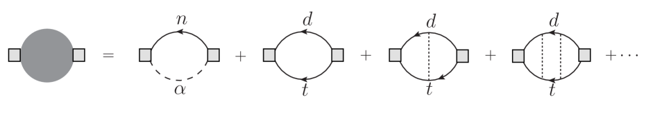
Including Coulomb corrections, the $dt\to n\alpha$ reaction is still described by the diagram in Fig. 4, but with two significant changes. The $dt$ entrance channel that connects these particles to the unstable, interacting ⁵He^∗ resonant Green’s function involves a point interaction. Hence, one effect of the Coulomb force between the $dt$ in the fusion process is to multiply the cross section by the square of the Coulomb wave function $\psi^{(C)}_{{\bf p}_{dt}}(0)$ at the origin. Thus the initial shaded box at the right in Fig. 4 must now contain $\psi^{(C)}_{{\bf p}_{dt}}(0)$ multiplying the coupling constant $g_{dt}$. The other effect of the Coulomb interactions is to modify the $dt$ loop graphs in the ${}^{5}{\rm He}^{*}$ resonant Green’s function by including arbitrary numbers of instantaneous Coulomb interactions as depicted in Fig. 5. These heuristic remarks are substantiated in Appendix C. Here we shall simply state and discuss the results of these Coulomb corrections.

The cross section involves the square of the amplitude and thus the square of the Coulomb wave function at the origin,

$$\left|\psi^{(C)}_{{\bf p}_{dt}}(0)\right|^{2}=\frac{2\pi\eta\,\exp\{-2\pi\eta\}}{1-\exp\{-2\pi\eta\}}\,.$$ (105)

This is essentially the familiar Gamow barrier penetration factor. For our deuteron-triton system, each with a single electron charge $e$, in ordinary cgs units,

$$\eta=\frac{e^{2}}{v_{dt}}=\frac{e^{2}m_{dt}}{p_{dt}}\,.$$ (106)

It is sometimes convenient to write

$$\eta=\frac{1}{b_{0}\,p_{dt}}\,,$$ (107)

with, in our units in which $\hbar=1$, $b_{0}$ is the Bohr radius for the $dt$ system,

$$b_{0}=\frac{1}{e^{2}m_{dt}}=24.04\,{\rm fm}=0.1218\,\frac{c}{\rm MeV}\,,$$ (108)

where $1\,{\rm fm}=10^{-13}\,{\rm cm}\,,$ and we have made use of $\hbar c=197.33\,{\rm MeV\,\,fm}$ in writing the last equality. In our theory, the Coulomb corrections to the intermediate state nuclear interactions appear only in the unstable field propagator. Thus, including all the Coulomb effects, the previous fusion cross section (100) becomes

$$\sigma_{dt\to n\alpha} =\frac{8}{9}\,4\pi\,m_{n\alpha}\,\frac{p_{n\alpha}^{5}}{v_{dt}}\,\frac{g^{2}_{dt}}{4\pi}\,\frac{g^{2}_{n\alpha}}{4\pi}\,$$

$$\times\left|\psi^{(C)}_{{\bf p}_{dt}}(0)\right|^{2}\,\left|G_{*}^{(C)}(W)\right|^{2}\,.$$ (109)

Here we use an additional superscript on the unstable particle’s interacting Green’s function $G_{*}^{(C)}(W)$ to note that it now includes the effect of the Coulomb interaction. The only effect of this interaction is on the previous $dt$ loop function (39) that contains charged particles, with

$$\Sigma_{dt}(W) \to\Sigma^{(C)}_{dt}(W)$$

$$=-i\,g_{dt}^{2}\,\int_{0}^{\infty}\,dt\,e^{iW\,t}\,\langle{\bf 0},t|{\bf 0},0\rangle^{(C)}_{dt\,\,\rm rel}\,,$$ (110)

corresponding to the infinite series of diagrams indicated in Fig. 5 containing the $dt$ intermediate state. Introducing a complete set of incoming wave intermediate eigenstates gives

$$\langle{\bf 0},t|{\bf 0},0\rangle^{(C)}_{dt\,\,\rm rel} =\int\frac{(d^{3}{\bf p}^{\prime})}{(2\pi)^{3}}\,\langle{\bf 0},t|{\bf p}^{\prime}\,{\rm in}\rangle^{(C)}_{dt\,\,\rm rel}\langle{\bf p}^{\prime}\,{\rm in}|{\bf 0},0\rangle^{(C)}_{dt\,\,\rm rel}$$

$$=e^{i(\epsilon_{d}+\epsilon_{t})t}\,\int\frac{(d^{3}{\bf p}^{\prime})}{(2\pi)^{3}}\,\exp\left\{-i\frac{{p^{\prime}}^{2}}{2m_{dt}}\,t\right\}\,$$

$$\times\left|\psi_{p^{\prime}}^{(C)}(0)\right|^{2}\,,$$ (111)

in which $m_{dt}$ is the reduced mass of the $dt$ system and $\psi_{p^{\prime}}^{(C)}(0)$ is the Coulomb wave function (105). Using the $dt$ relative momentum $p_{dt}$ so that the energy in the center of mass is given by

$$W+\epsilon_{d}+\epsilon_{t}=\frac{p_{dt}^{2}}{2m_{dt}}\,,$$ (112)

performing the time integration in Eq. (110) with the decomposition (111), and also performing the angular part of the momentum integral produces

$$\overline{\Sigma^{(C)}}_{dt}(W) =g_{dt}^{2}\,\frac{m_{dt}}{\pi^{2}}\,\int_{0}^{\infty}dp^{\prime}\,\left|\psi^{(C)}_{p^{\prime}}(0)\right|^{2}$$

$$\times\frac{{p^{\prime}}^{2}}{p_{dt}^{2}-{p^{\prime}}^{2}+i0^{+}}\,.$$ (113)

At large momenta, the Coulomb wave function approaches the free-particle limit, $p^{\prime}\to\infty\,:\,\psi^{(C)}_{p^{\prime}}(0)\to 1$. Hence the integral here does not converge at large momenta. We have noted this divergence by temporarily placing an overline on the function. Previously, we dealt with this convergence problem by employing the dimensional continuation method which simply removes this divergence in three dimensions. Here, however, we have an integrand involving the square of the Coulomb wave function and the application of the dimensional continuation method is more complex. There is no real problem here because the divergence produces an additional constant that is simply removed by an additive renormalization of the energy $\epsilon_{*}$, a renormalization which we shall assume has been implicitly performed. Thus we simply subtract the asymptotic limit and replace

$$\frac{{p^{\prime}}^{2}}{p_{dt}^{2}-{p^{\prime}}^{2}+i0^{+}} \to\frac{{p^{\prime}}^{2}}{p_{dt}^{2}-{p^{\prime}}^{2}+i0^{+}}+1$$

$$=\frac{p_{dt}^{2}}{p_{dt}^{2}-{p^{\prime}}^{2}+i0^{+}}\,,$$ (114)

remove the overline from the self-energy function, and write

$$\Sigma^{(C)}_{dt}(W) =g_{dt}^{2}\frac{m_{dt}p_{dt}^{2}}{\pi^{2}}\int_{0}^{\infty}dp^{\prime}\,\frac{\left|\psi^{(C)}_{p^{\prime}}(0)\right|^{2}}{p_{dt}^{2}-{p^{\prime}}^{2}+i0^{+}}.$$ (115)

This shows explicitly that the Coulomb-corrected self-energy function $\Sigma^{(C)}_{dt}(W)$ is the boundary value of a function that is analytic in the upper half complex $p_{dt}^{2}/2m_{dt}$ plane. This is because it is the Fourier transform of a retarded, causal response function. We conclude that the real part of $\Sigma^{(C)}_{dt}(W)$ must accompany its imaginary part to keep the proper, complete analytic function. For physical, real energies we may use

$${\rm Im}\,\frac{1}{p_{dt}^{2}-{p^{\prime}}^{2}+i0^{+}} =-\pi\delta(p_{dt}^{2}-{p^{\prime}}^{2})$$

$$=-\frac{\pi}{2p_{dt}}\,\delta(p_{dt}-p^{\prime})$$ (116)

to compute the imaginary part,

$${\rm Im}\,\Sigma^{(C)}_{dt}(W) = -g_{dt}^{2}\,\frac{m_{dt}\,p_{dt}}{2\pi}\,\left|\psi^{(C)}_{p_{dt}}(0)\right|^{2}\,.$$ (117)

To have an explicit representation of the real part, we use

$$\left|\psi^{(C)}_{p^{\prime}}(0)\right|^{2}=\frac{2\pi\eta^{\prime}}{\exp\{2\pi\eta^{\prime}\}-1}\,,$$ (118)

and change the integration variable to $t=\eta^{\prime}=1/(p^{\prime}\,b_{0})\,,$ obtaining

$$\Sigma^{(C)}_{dt}(W) =g_{dt}^{2}\frac{2m_{dt}}{\pi b_{0}}\int_{0}^{\infty}dt\,t\frac{1}{t^{2}-\eta^{2}+i0^{+}}$$

$$\times\frac{1}{\exp\{2\pi t\}-1},$$ (119)

in which $\eta=1/(p_{dt}\,b_{0})\,.$ This new form of the self-energy function is simply related to the $\psi$ function — the logarithmic derivative of the $\Gamma$ function — because of the integral representation

$$\psi(z) =\ln z-\frac{1}{2z}-2\int_{0}^{\infty}dt\,t\,\frac{1}{t^{2}+z^{2}}$$

$$\times\frac{1}{\exp\{2\pi\,t\}-1},$$ (120)

where it is assumed that ${\rm Re}z>0$. Hence

$$\Sigma^{(C)}_{dt}(W)=-g_{dt}^{2}\frac{m_{dt}}{\pi b_{0}}\left[\psi(i\eta)-\ln\eta-\frac{\pi}{2}i-\frac{i}{2\eta}\right],$$ (121)

which gives the real part

$${\rm Re}\,\Sigma^{(C)}(W)=-\frac{g_{dt}^{2}}{4\pi}\,\Delta(W)\,,$$ (122)

where

$$\Delta(W)=\frac{4m_{dt}}{b_{0}}\left[{\rm Re}\,\psi(i\eta)-\,\ln\,\eta\right]\,,$$ (123)

We pause to record some formulae that can prove to be useful checks on numerical computations. It follows from the standard series development of the $\psi$ function that

$${\rm Re}\,\psi(i\eta)=-\gamma+\sum_{k=1}^{\infty}\frac{1}{k}\frac{\eta^{2}}{k^{2}+\eta^{2}}\,,$$ (124)

which gives the small $\eta$ behavior

$${\rm Re}\,\psi(i\eta) =-\gamma+\zeta(3)\,\eta^{2}+\dots$$

$$\simeq-0.5772157+1.20206\,\eta^{2}\,.$$ (125)

Moreover,

$${\rm Re}\,\psi(i\eta)=-\gamma+\frac{\eta^{2}}{1+\eta^{2}}+\frac{1}{2}\frac{\eta^{2}}{4+\eta^{2}}+R(\eta)\,,$$ (126)

where we have the bound

$$\left|R(\eta)\right|\leq B(\eta) =\eta^{2}\,\sum_{k=3}^{\infty}\frac{1}{k^{3}}=\eta^{2}\,\left[\zeta(3)-1-\frac{1}{8}\right]$$

$$=\eta^{2}\left[0.07706\right]\,.$$ (127)

The large $\eta$ limit gives

$${\rm Re}\,\psi(i\eta)-\ln\eta=\frac{1}{12\,\eta^{2}}-\frac{1}{120}\,\frac{1}{\eta^{4}}+\dots\,.$$ (128)

The inverse unstable field Green’s function now reads

$$G_{*}^{(C)\,-1}(W)=-(W+\epsilon_{*})-\Sigma^{(C)}_{dt}(W)-\Sigma_{n\alpha}(W)\,,$$ (129)

with $\Sigma^{(C)}_{dt}(W)$ the function that we have just computed, while

$$\Sigma_{n\alpha}(W) = -i\,\frac{2}{3}\,\frac{g_{n\alpha}^{2}}{4\pi}\,m_{n\alpha}p_{n\alpha}^{5}$$ (130)

is as before.

The absolute square of the unstable field Green’s function that is needed for the fusion cross section (109) is produced by the trivial notational change $\Sigma_{dt}\to\Sigma^{(C)}_{dt}$ in the formula (103), producing

$$\left|G_{*}^{(C)}(W)\right|^{-2}$$

$$=\Bigg{[}\frac{p_{dt}^{2}}{2m_{dt}}-E_{*}-\frac{g_{dt}^{2}}{4\pi}\Delta(W)\Bigg{]}^{2}$$

$$+\Bigg{[}\frac{g_{dt}^{2}}{2\pi}m_{dt}p_{dt}\left|\psi^{(C)}_{p_{dt}}(0)\right|^{2}+\frac{g_{n\alpha}^{2}}{6\pi}m_{n\alpha}p_{n\alpha}^{5}\Bigg{]}^{2}$$ (131)

in which we again write the unrenormalized energy of the unstable particle in terms of the initial $dt$ energy as

$$E_{*}=\epsilon_{d}+\epsilon_{t}-\epsilon_{*}\,.$$ (132)

V Conclusion and Discussion

We have demonstrated that an excellent description of the $dt\to n\alpha$ reaction in the resonance region is obtained with an effective quantum field theory that entails only the interaction of the initial and final particles $dt$ and $n\alpha$ with an unstable ⁵He^∗ $3/2^{+}$ unstable field. The fit, with a $\chi^{2}$ per degree-of-freedom less than unity, is achieved with just three parameters: the energy of the ⁵He^∗ resonance $E_{*}$, and the two coupling parameters $g_{dt}$ and $g_{n\alpha}$. We have calculated the Coulomb corrections exactly in Sec. IV and taken into account their effect on both the incoming $dt$ particles and on the strong interactions which transmute these particles into the final $n\alpha$ particles.

It is worthwhile noting that, early on, we found that the $dt\to n\alpha$ resonance could not be fit by using an intermediate $3/2^{+}$ unstable field which had the right sign free-particle Lagrangian. The fit was so poor that a $\chi^{2}$ value to describe it is not meaningful. Roughly, if the parameters were adjusted to fit the maximum of the cross section resonance, then the data around half maximum were about 30% above the fit. This result led us to add an additional contact interaction that coupled the initial and final particles in a $3/2^{+}$ state. We chose this form of the contact interaction so that it would enter into the self-energy function of the $3/2^{+}$ field’s Green’s function and hence would be a candidate to alter the resonance shape produced by the theory. As described in Eq. (23), the final $n\alpha$ particles are produced in a $3/2^{+}$ state by the field combination $\bm{\Psi}_{\alpha\,n}$ and hence the contact interaction was chosen to have the form

$$\lambda\left[\bm{\Psi}^{\dagger}_{\alpha\,n}\cdot\bm{\phi}_{d}\,\,\psi_{t}+\psi^{\dagger}_{t}\,\,\bm{\phi}^{\dagger}_{d}\cdot\bm{\Psi}_{\alpha\,n}\right]\,.$$ (133)

As should be expected, the introduction of the additional free parameter $\lambda$ improved the fit. However, the improvement was not significant. With the parameters again chosen to have the resonance maximum fitted, the data around half maximum were now about 20% above the fit. Therefore, we reverted to the simple, previous single interaction with an intermediate unstable field, and changed the sign of its free-particle propagation to achieve the excellent description of the $dt$ fusion reaction that is presented in this paper. The quality of this fit, about 1% deviation for most of the data points, was a dramatic improvement over the other work just discussed.

The relationship between the effective field theory applied here and the $R$-matrix approach is presented in the following paper BHP . It establishes an identity between the effective field theory approach and that of the $R$ matrix, in the limit that the $R$-matrix channel radii go to zero. In this limit, the $R$-matrix parameterization provides an excellent fit of the data when generalized to allow for “unphysical” negative values of the reduced widths. These unphysical couplings are directly related to the wrong-sign free-particle Lagrange function used in the present work. This is a promising indication that carrying out a multichannel, many-resonance effective field theory description of light nuclear reaction data is possible by suitably generalizing current $R$-matrix methods and codes that are already in use.

Appendix A Galilean Invariance

The consequences of translational and rotational invariance are obvious. The consequences of Galilean invariance — the invariance of the theory under ‘boosts’ to a moving coordinate frame — are less obvious, although perhaps they are clear once they have been derived. Here we sketch out the derivation of some of these consequences.

We denote the generator of boosts to moving frames by ${\bf G}$. It has the construction

$${\bf G}={\bf P}\,t-M\,{\bf R}(t)\,,$$ (134)

where, for a general set $\{\chi_{a},\chi^{\dagger}_{a}\}$ of non-relativistic fields,

$${\bf P}={\sum}_{a}\int(d^{3}{\bf r})\,\chi_{a}^{\dagger}({\bf r},t)\,\frac{1}{i}\nabla\,\chi_{a}({\bf r},t)$$ (135)

is the total momentum operator of the system, and

$$M\,{\bf R}(t)={\sum}_{a}\int(d^{3}{\bf r})\,\chi_{a}^{\dagger}({\bf r},t)\,m_{a}\,{\bf r}\,\chi_{a}({\bf r},t)$$ (136)

defines a the center-of-mass operator ${\bf R}$, with $m_{a}$ the kinematical mass of the particle, bound state, or resonance created and annihilated by the $a$-th field and $M={\sum}_{a}\,m_{a}$ is the total mass of all these (perhaps quasi-) particles. The kinematical mass $m_{a}$ is the mass that appears in the kinetic energy part of the Hamiltonian density $\chi^{\dagger}_{a}(-\nabla^{2}/2m_{a})\chi_{a}$ for the $a$-th field.

The continued iteration of the infinitesimal Galilean boosts yields the unitary transformation

$$U({\bf v})=\exp\left\{i\,{\bf G}\cdot{\bf v}\right\}=\exp\left\{i\left[{\bf P}\,t-M\,{\bf R}(t)\right]\cdot{\bf v}\right\}$$ (137)

to a frame moving with the finite velocity ${\bf v}$. Standard methods now show that the response of a field $\chi_{a}$ to a finite Galilean boost is given by

$$\chi_{a}({\bf r},t) \to U^{-1}({\bf v})\chi_{a}({\bf r},t)U({\bf v})$$

$$=\exp\left\{-im_{a}\left[{\bf r}\cdot{\bf v}+\frac{1}{2}{\bf v}^{2}t\right]\right\}$$

$$\times\chi_{a}({\bf r}+{\bf v}t,t).$$ (138)

We shall make use of three implications of this transformation.

Nucleons can be put into bound or resonant states. Hence the effective field theory can contain interactions of the schematic form

$$H_{int}\sim\int(d^{3}{\bf r})\,\chi_{b_{n}}^{\dagger}\cdots\chi_{b_{1}}^{\dagger}\,\chi_{a_{m}}\cdots\chi_{a_{1}}\,.$$ (139)

In view of the response of the individual fields given by Eq. (138), Galilean invariance requires that

$$m_{b_{n}}+\dots+m_{b_{1}}=m_{a_{m}}+\dots+m_{a_{1}}\,.$$ (140)

Thus, for example, the inertial mass of the deuteron is the sum of the neutron and proton masses, $m_{d}=m_{n}+m_{p}$, the triton mass is $m_{t}=2m_{n}+m_{p}$, and the alpha mass is $m_{\alpha}=2m_{n}+2m_{p}$.

The second consequence of Galilean invariance that we mention is that a generic free-particle Lagrangian must be of the form

$$L_{\rm\scriptscriptstyle A} =\int(d^{3}{\bf r})\chi_{\rm\scriptscriptstyle A}^{\dagger}({\bf r},t)$$

$$\times\left[i\frac{\partial}{\partial t}-\frac{1}{2m_{\rm\scriptscriptstyle A}}\,\left(\frac{1}{i}\nabla\right)^{2}-\epsilon_{\rm\scriptscriptstyle A}\right]\chi_{\rm\scriptscriptstyle A}({\bf r},t)\,.$$ (141)

Galilean invariance requires that the relative signs of the time and spatial derivatives must appear as they are shown here.

The final application that we need involves field derivatives. To obtain Galilean invariant interactions, we need field combinations with derivatives that undergo a simple phase change under Galilean transformations. This does not happen with a single derivative of a single field. However, with a pair of fields $\chi_{a}$, $\chi_{b}$, we can define a derivative operation

$${\cal P}^{k}_{ba}=\frac{m_{ab}}{m_{a}}\frac{1}{i}\stackrel{{\scriptstyle\rightarrow}}{{\nabla}}^{k}-\frac{m_{ab}}{m_{b}}\frac{1}{i}\stackrel{{\scriptstyle\leftarrow}}{{\nabla}}^{k}\,,$$ (142)

in which $\rightarrow$ calls for the derivative to act to the right, and $\leftarrow$ calls for the derivative to act to the left. Here

$$m_{ab}=\frac{m_{a}\,m_{b}}{M_{ab}}\,,$$ (143)

is the reduced mass of the $a,b$ pair with

$$M_{ab}=m_{a}+m_{b}$$ (144)

the total mass. It is now easy to see that

$$U^{-1}({\bf v})\chi_{b}({\bf r},t){\cal P}^{k}_{ba}\chi_{a}({\bf r},t)U({\bf v})=$$

$$e^{-i\,(m_{b}+m_{a})\,[{\bf r}\cdot{\bf v}+\frac{1}{2}\,{\bf v}^{2}\,t]}\chi_{b}({\bf r}+{\bf v}t,t)$$

$$\times{\cal P}^{k}_{ba}\chi_{a}({\bf r}+{\bf v}t,t),$$ (145)

which is the desired transformation law.

Appendix B Spin Structure

Here we shall describe some algebraic properties of the spin matrices that are needed in the text. We shall keep to our $\hbar=1$ convention so as to simplify the notation. The action on any field $\chi$ of an infinitesimal rotation generated by the field operator angular momentum ${\bf J}$ is given by

$$\left\{{\bf L}+{\bf S}\right\}\chi({\bf r},t)=\left[\chi({\bf r},t),{\bf J}\right]\,,$$ (146)

in which

$${\bf L}={\bf r}\times\frac{1}{i}\nabla$$ (147)

are the orbital angular momentum differential operators and ${\bf S}$ are the spin matrices. The structure of the rotation group is conveyed by

$$\left[J^{k},J^{l}\right]=i\epsilon^{klm}J^{m}\,,$$ (148)

where $\epsilon^{klm}$ is the completely antisymmetrical numerical tensor associated with vector cross product, with $\epsilon^{123}=1$. This numerical tensor satisfies the “double cross” relation

$$\epsilon^{klm}\epsilon^{kpq}=\delta^{lp}\delta^{mq}-\delta^{lq}\delta^{mp}\,.$$ (149)

Since $L^{k}$ acts on the coordinates of the field while $S^{k}$ acts on the (notationally suppressed) components of the fields, $L^{k}$ and $S^{k}$ commute amongst each other, while

$$\left[L^{k},L^{l}\right]=i\epsilon^{klm}L^{m}\,,$$ (150)

and

$$\left[S^{k},S^{l}\right]=i\epsilon^{klm}S^{m}\,.$$ (151)

We turn now to examine the spin matrices ${\bf S}$ for spin $s$ with $s=1/2\,,\,1\,,\,3/2$. These matrices must obey the commutator (151) and have the square

$${\bf S}^{2}=s(s+1)\,.$$ (152)

B.0.1 Spin $1/2$

For spin one-half,

$$\bm{S}=\frac{1}{2}\bm{\sigma}\,,$$ (153)

in which $\sigma^{k}$ are the familiar Hermitian Pauli matrices that obey

$$\sigma^{k}\sigma^{l}=\delta^{kl}+i\epsilon^{klm}\sigma^{m}\,.$$ (154)

The antisymmetrical part of this constraint implies that the spin $1/2$ matrices $S^{k}$ satisfy the angular momentum commutation relation (151) while setting $k=l$ and summing over these identified indices from 1 to 3 shows that

$${\bf S}^{2}=\frac{3}{4}=\frac{1}{2}\left(\frac{1}{2}+1\right)\,,$$ (155)

which identifies the spin value $1/2$.

B.0.2 Spin $1$

We write the spin matrices for spin one as

$$\bm{S}=\bm{{\cal S}}\,.$$ (156)

The latter are given by

$$\left({\cal S}^{k}\right)^{lm}=i\epsilon^{lkm}\,,$$ (157)

since one can easily verify from the relation (149) that the angular momentum commutation relation (151) holds and that

$$\bm{{\cal S}}^{2}=1\,(1+1)=2$$ (158)

B.0.3 Spin $3/2$

The combination of spin $1/2$ and spin $1$ is described by the spin matrix

$$\bm{{S}}=\frac{1}{2}\bm{{\sigma}}+\bm{{\cal S}}\,.$$ (159)

This matrix obviously obeys the angular momentum commutator (151). But we need a constraint to keep to the spin $3/2$ subspace. To obtain this constraint, we note that the Pauli result (154) and the properties of the spin-one matrix noted above imply the characteristic equation

$$\left(\bm{\sigma}\cdot\bm{{\cal S}}\right)^{2}+\left(\bm{\sigma}\cdot\bm{{\cal S}}\right)-2=0\,.$$ (160)

The eigenvalues of the matrix, which we denote by a prime, must obey this characteristic matrix equation, and hence they are given by

$$\left(\bm{\sigma}\cdot\bm{{\cal S}}\right)^{\prime}=\left\{\begin{array}[]{c}-2\,,\\ +1\,.\end{array}\right.$$ (161)

Therefore we have

$${\bf S}^{2} =\frac{3}{4}+2+\bm{\sigma}\cdot\bm{{\cal S}}$$

$$=\left\{\begin{array}[]{cc}\frac{1}{2}\left(\frac{1}{2}+1\right),&{\rm for}\,\left(\bm{\sigma}\cdot\bm{{\cal S}}\right)^{\prime}=-2,\\ &\\ \frac{3}{2}\left(\frac{3}{2}+1\right),&{\rm for}\,\left(\bm{\sigma}\cdot\bm{{\cal S}}\right)^{\prime}=\hphantom{-}1;\end{array}\right.$$ (165)

the eigenvalues $-2$ and $1$ of the matrix $\bm{\sigma}\cdot\bm{{\cal S}}$ correspond to spins $s=1/2$ and $s=3/2$.

We need the matrix $P_{3/2}$ that projects into the $s=3/2$ subspace. A little computation utilizing the characteristic equation (160) shows that

$$P_{3/2}=\frac{1}{3}\left\{\bm{\sigma}\cdot\bm{{\cal S}}+2\right\}$$ (166)

obeys

$$\left(\bm{\sigma}\cdot\bm{{\cal S}}\right)P_{3/2}=P_{3/2}=P_{3/2}\left(\bm{\sigma}\cdot\bm{{\cal S}}\right)\,,$$ (167)

and

$$P_{3/2}^{\,\,\,2}=P_{3/2}\,,$$ (168)

so that it is indeed the correct projection matrix. Writing out the components gives

$$P_{3/2}^{lm}=\frac{1}{3}\left\{\sigma^{k}\,i\,\epsilon^{lkm}+2\,\delta^{lm}\right\}\,.$$ (169)

In view of the result (165), a spin $3/2$ field $\psi_{3/2}$ must obey the constraint

$$\bm{\sigma}\cdot\bm{{\cal S}}\,\psi_{3/2}=\psi_{3/2}\,.$$ (170)

and if this constraint is obeyed, the field contains only spin $3/2$. To obtain an equivalent constraint that is algebraically simpler, we note that

$$\sigma^{l}\,\left(\bm{\sigma}\cdot\bm{{\cal S}}\right)^{lm} = -\epsilon^{lkn}\,\epsilon^{lkm}\,\sigma^{n}=-2\,\sigma^{m}\,.$$ (171)

Hence, in view of Eq. (167),

$$\sigma^{l}\,\left(\bm{\sigma}\cdot\bm{{\cal S}}\right)^{lm}P_{3/2}^{mn}=-2\sigma^{m}\,P_{3/2}^{nm}=\sigma^{m}\,P_{3/2}^{nm}\,;$$ (172)

whence

$$\sigma^{l}\,P_{3/2}^{lm}=0\,,$$ (173)

and similarly,

$$P_{3/2}^{lm}\,\,\sigma^{m}=0\,.$$ (174)

Therefore,

$$\bm{\sigma}\cdot\bm{\psi}_{3/2}({\bf r},t)=0=\bm{\psi}_{3/2}^{\dagger}({\bf r},t)\cdot\bm{\sigma}\,,$$ (175)

constrain $\bm{\psi}_{3/2}$ and $\bm{\psi}_{3/2}^{\dagger}$ to contain only spin $3/2$.

In the text, we need the spin $3/2$ combination of $n$, $\alpha$ fields that couple to the ${3/2}^{+}$ ${}^{5}{\rm He}^{*}$ resonant state. The composition of the ${3/2}^{+}$ state from the ${1/2}^{+}$ neutron and $0^{+}$ alpha requires that the parity of the relative orbital state of the $n$ , $\alpha$ pair be even, which is to say that the orbital angular momentum $l$ be an even integer, with $l=2$, the only possibility in virtue of the rules of angular momentum addition. The differential operation

$${\cal T}^{kl}_{\alpha n}={\cal P}^{k}_{\alpha n}{\cal P}^{l}_{\alpha n}-\frac{1}{3}\,\delta^{kl}\,{\cal P}^{m}_{\alpha n}{\cal P}^{m}_{\alpha n}$$ (176)

transforms as $l=2$. Here, ${\cal P}^{k}_{\alpha n}$ is defined by Eq. (142) and a proof akin to that with Eq. (145) shows that

$$\Psi^{l}_{\alpha n}({\bf r},t)=\phi_{\alpha}({\bf r},t)\,{\cal T}^{lm}_{\alpha n}\,\sigma^{m}\,\psi_{n}({\bf r},t)$$ (177)

has the correct Galilean transformation law. Using the Pauli spin formula (154) and the symmetry ${\cal T}^{lk}_{\alpha n}=+{\cal T}^{kl}_{\alpha n}$ we compute

$$\sigma^{k}\Psi^{k}_{\alpha n}({\bf r},t)=\phi_{\alpha}({\bf r},t)\,\delta^{kl}{\cal T}^{kl}_{\alpha n}\,\psi_{n}({\bf r},t)=0\,.$$ (178)

Hence, in view of Eq. (175) and the discussion following it, we conclude that $\Psi^{k}({\bf r},t)$ does indeed contain only spin $3/2$.

Appendix C Coulomb corrections

To place our work in context, we first briefly review the case in which there are only strong interactions with no Coulomb corrections. The four-point $n\alpha\,dt$ Green’s function is the vacuum expectation value of a time-ordered product,

$$G_{n\alpha\,dt}(x^{\prime}_{n},x^{\prime}_{\alpha};x_{d},x_{t})$$

$$=i^{2}\left\langle 0\left|\left(\psi_{n}(x^{\prime}_{n})\phi_{\alpha}(x^{\prime}_{\alpha})\phi_{d}^{\dagger}(x_{d})\psi^{\dagger}_{t}(x_{t})\right)_{+}\right|0\right\rangle\,,$$ (179)

in which the space time coordinate $x$ is a short-hand notation for ${\bf r},t$. It has the decomposition

$$G_{n\alpha\,dt}(x^{\prime}_{n},x^{\prime}_{\alpha};x_{d},x_{t}) =\int(d^{4}\bar{x}_{n})(d^{4}\bar{x}_{\alpha})(d^{4}\bar{x}_{d})(d^{4}\bar{x}_{t})\,G_{n}(x^{\prime}_{n}-\bar{x}_{n})\,G_{\alpha}(x_{\alpha}^{\prime}-\bar{x}_{\alpha})$$

$$\times\Gamma_{n\alpha\,dt}(\bar{x}_{n},\bar{x}_{\alpha},\bar{x}_{d},\bar{x}_{t})\,G_{d}(\bar{x}_{d}-x_{d})\,G_{t}(\bar{x}_{t}-x_{t})\,.$$ (180)

Here $\Gamma_{n\alpha\,dt}(\bar{x}_{n},\bar{x}_{\alpha},\bar{x}_{d},\bar{x}_{t})$ contains only connected graphs. In our non-relativistic theory, the single-particle propagators contain no self-energy corrections and thus have the generic, form of the time retarded functions

$$G(x-x^{\prime}) =\theta\left(t-t^{\prime}\right)\int\frac{(d^{3}{\bf p})}{(2\pi)^{3}}e^{i{\bf p}\cdot({\bf r}-{\bf r}^{\prime})-iE({\bf p})(t-t^{\prime})}$$

$$=\theta\left(t-t^{\prime}\right)\langle{\bf r},t|{\bf p}^{\prime},t^{\prime}\rangle^{(0)},$$ (181)

where in the second line we denote the free-particle quantum-mechanical transformation function by the superscript $(0)$. The reaction amplitude involves the asymptotic early and late time limits $t_{d}=t_{t}\to-\infty$ and $t_{n}=t_{\alpha}\to+\infty$ and the identification of the propagator momenta ${\bf p}$ with the initial momenta, ${\bf p}_{d}$ and ${\bf p}_{t}$ and final momenta, ${\bf p}_{n}$ and ${\bf p}_{\alpha}$, by the appropriate Fourier transformation. Therefore, aside from conventional factors and overall delta functions of energy and momentum conservation, the reaction amplitude $T_{n\alpha\,dt}({\bf p}_{n},{\bf p}_{\alpha};{\bf p}_{d},{\bf p}_{t})$ involves a Fourier transform of $\Gamma_{n\alpha\,dt}(\bar{x}_{n},\bar{x}_{\alpha},\bar{x}_{d},\bar{x}_{t})$ .

We now consider effect that Coulomb corrections have on the charged initial $dt$ state. When Coulomb interactions are present, there are instantaneous Coulomb exchanges in the propagation of the initial $dt$ particles before strong interactions operate. Thus the product of the two initial free-particle propagators $\,G_{d}(\bar{x}_{d}-x_{d})\,G_{t}(\bar{x}_{t}-x_{t})$ in Eq. (180 must be replaced by the four-point $dt$ Green’s function that includes the Coulomb interaction. The general reaction amplitude involves the identification of the two initial times, $t_{d}=t_{t}$. Our theory, in which the strong interactions are represented by the unstable, s-channel intermediate field $\psi_{*}^{\dagger}$ that has a local coupling to the $d$ and $t$ fields, forces the identification $\bar{x}_{d}=\bar{x}_{t}$ or $\bar{\bf r}_{d}=\bar{\bf r}_{t}$ and $\bar{t}_{d}=\bar{t}_{t}$, with $\bar{t}_{d}>t_{d}$. Hence the required four-point Coulomb Green’s appears in the restricted form

$$-G^{(C)}_{dt}({\bf r}_{d},\bar{t}_{d},{\bf r}_{t}={\bf r}_{d},\bar{t}_{t}=\bar{t}_{d};{\bf r}_{d},t_{d},{\bf r}_{t},t_{t}=t_{t})$$

$$=\left\langle 0\left|\psi_{d}(\bar{\bf r}_{d},\bar{t})\,\psi_{t}({\bf r}_{d},t_{d})\,\psi_{t}^{\dagger}({\bf r}_{t},t_{d})\,\psi_{d}^{\dagger}({\bf r}_{d},t_{d})\right|0\right\rangle^{(C)}$$

$$=\langle\bar{\bf r}_{d}=\bar{\bf r}_{t},\bar{t}_{d}|{\bf r}_{d},{\bf r}_{t},t_{d}\rangle^{(C)}\,.$$ (182)

The second line here follows from the usual non-relativistic theory where a field operator $\psi^{\dagger}$ acting to the right adds a single particle to the state, and an operator $\psi$ acting to the left adds a particle. We have noted that the transition amplitude involves taking the spatial Fourier transform.

Hence, passing to the transition amplitude involves $\langle\bar{\bf r}_{d}=\bar{\bf r}_{t},\bar{t}_{d}|{\bf p}_{d},{\bf p}_{t},t_{d}\rangle^{(C)}$. On introducing relative and center-of-mass coordinates, this becomes

$$\langle\bar{\bf r}_{d}=\bar{\bf r}_{t},\bar{t}_{d}|{\bf p}_{d},{\bf p}_{t},t_{d}\rangle^{(C)}$$

$$=\langle{\bf r}_{\rm rel}=0|{\bf p}_{dt}\rangle^{(C)}\langle{\bf r}_{d}|{\bf P}_{dt}\rangle^{(0)}e^{-iE(\bar{t}_{d}-t_{d})}.$$ (183)

Here ${\bf p}_{dt}$ is the relative momentum of the $dt$ (which is the same notation as used in the text), ${\bf P}_{dt}$ is the total momentum of this pair of particles, and $E$ is the total energy in the initial state. Now

$$\langle{\bf r}_{\rm rel}=0|{\bf p}_{dt}\rangle^{(C)}=\psi^{(C)}_{{\bf p}_{dt}}(0)$$ (184)

is precisely the Coulomb wave function at the origin introduced in the text. Only this factor alters the Coulomb transformation function (183) from that of a free particle:

$$\langle\bar{\bf r}_{d}=\bar{\bf r}_{t},\bar{t}_{d}|{\bf p}_{d},{\bf p}_{t},t_{d}\rangle^{(C)}$$

$$=\psi^{(C)}_{{\bf p}_{dt}}(0)\,\langle\bar{\bf r}_{d}=\bar{\bf r}_{t},\bar{t}_{d}|{\bf p}_{d},{\bf p}_{t},t_{d}\rangle^{(0)}\,.$$ (185)

Hence, the ‘reduction formula’ for the transition amplitude with Coulomb as well as strong interactions is the same as that for the amplitude with only strong interactions and no Coulomb corrections except for the overall multiplication of the $\psi^{(C)}_{{\bf p}_{dt}}(0)$ factor corresponding to initial Coulomb interactions previous to the first strong interaction. Of course, there are additional internal Coulomb corrections to the strong interactions. For our theory, these appear as multiple instantaneous Coulomb exchanges between the $d$ and the $t$ in the $dt$ loop that contributes to the unstable ⁵He^∗ Green’s function as shown in Fig. 5.

References

- (1) L. S. Brown, Quantum Field Theory, (Cambridge University Press, Cambridge, 1992).
- (2) E. Fermi, Ricerca Scientifica 7, 13 (1936), Sec. 10; reprinted in E. Fermi, Collected Papers, Vol. I, Ed. by E. Amaldi et al., Univ. of Chicago Press (1962).
- (3) J. Schwinger, Particles, Sources, And Fields, Vol. II, Sec. 4-7 (Addison-Wesley Pub. Co., Reading MA. 1973.)
- (4) S. Weinberg, Phys. Lett. B, 251, 288 (1990).
- (5) G. M. Hale, L. S. Brown, and M. W. Paris, Phys. Rev. C (following paper).
- (6) A preliminary sketch of the field theory method of computing nuclear fusion rates in a plasma appears in L. S. Brown, D. C. Dooling, and D. L. Preston, J. Phys. A: Math. Gen. 39, 4475 (2006).
- (7) H.-S. Bosch and G. M. Hale, Nucl. Fusion 32, 611 (1992).
- (8) W. R. Arnold, J. A. Phillips, G. A. Saywer, E. J. Stovall, Jr., and J. L. Tuck, Phys. Rev. 93, 483 (1954).
- (9) N. Jarmie, R. E. Brown, and R. A. Hardekopf, Phys. Rev. C 29, 2031 (1984).
- (10) R. E. Brown, N. Jarmie, and G. M. Hale, Phys. Rev. C 35, 1999 (1987).
- (11) H. V. Argo, R. F. Taschek, H. M. Agnew, A. Hemmendinger, and W. T. Leland, Phys. Rev. 87, 612 (1952).
- (12) D. B. Kaplan, Nuc. Phys. B 494, 471 (1997).
- (13) W. Rarita and J. Schwinger, Phys. Rev. 69, 61 (1941).
- (14) A. Erdélyi, et al., Higher Transcendental Functions (Bateman Manuscript Project), Vol I. McGraw-Hill Book Co., Inc., New York, 1953.
- (15) I. S. Gradshteyn and I. M. Ryzhik, Table of Integrals, Series, and Products, 6 th ed., Academic Press, San Diego, 2000.