Distribution-Free Tests for Sparse Heterogeneous Mixtures
Abstract
We consider the problem of detecting sparse heterogeneous mixtures from a nonparametric perspective, and develop distribution-free tests when all effects have the same sign. Specifically, we assume that the null distribution is symmetric about zero, while the true effects have positive median. We evaluate the precise performance of classical tests for the median (t-test, sign test) and classical tests for symmetry (signed-rank, Smirnov, total number of runs, longest run tests) showing that none of them is asymptotically optimal for the normal mixture model in all sparsity regimes. We then suggest two new tests. The main one is a form of Higher Criticism, or Anderson-Darling, test for symmetry. It is shown to be asymptotically optimal for the normal mixture model, and other generalized Gaussian mixture models, in all sparsity regimes. Our numerical experiments confirm our theoretical findings.
MSC 2010: 62G10, 62G32, 62G20.
Keywords: mixture detection, distribution-free tests, higher criticism, Anderson-Darling test, sign test, signed-rank test, run tests, cumulative sum tests.
1 Introduction
Detecting heterogeneity in data has been an emblematic problem in statistics for decades. We consider the following stylized variant. We observe a sample , and want to test
| (1) | ||||
| (2) |
is the null distribution, is the non-null effects distribution, and and are the fraction and magnitude of the non-null (here positive) effects.
This testing problem could model a clinical trial where each one of subjects is given one of two treatments, or , say for high-blood pressure, for a period of time, and then given the other treatment for another period of time. In that setting, would be the decrease in blood pressure in subject under treatment minus that under treatment . The model above would be appropriate if treatment is expected to be at least as effective as treatment , and strictly more effective in a (possibly small) fraction of the subjects. The model may also be relevant in a multiple testing situation where the th test rejects for large values of the statistic . For example, in a gene expression experiment comparing a treatment and control group, a test statistic is computed for each gene; typically, the fraction of genes that are differentially expressed — which corresponds to non-null effects — is presumed to be small.
When the model is fully known, the likelihood ratio test (LRT) is the most powerful test. Our goal is to devise adaptive, distribution-free tests111In our context, a test is distribution-free (aka nonparametric) if its level does not depend on the null distribution , as long as is continuous and symmetric about zero. that can compete with the LRT without knowledge of the model specifics. For this to be possible, we assume that is symmetric about zero. Our standing assumptions are:
-
(A1)
is continuous and symmetric about zero (i.e., for all ), while is continuous and has zero median.
We emphasize that we do not consider the null and alternative hypotheses as composite hypotheses. A minimax approach in that direction may require more restrictions on or , and would tend to focus the problem on particularly difficult distributions to test.
We study the testing problem (1)-(2) in an asymptotic setting where . (All the limits that appear in the paper are as , unless otherwise specified.) We focus on the situation where the fraction of positive effects , distinguishing between two main asymptotic regimes:
| (3) |
We say that a test based on a statistic is asymptotically powerful (resp. powerless) if the total variation distance between the distribution of under the null (1) and under the alternative (2) tends to 2 (resp. 0) when . (Using this terminology, we avoid specifying complicated critical values.)
1.1 A benchmark: the generalized Gaussian mixture model
The normal location model is often a benchmark for assessing the power loss for using distribution-free tests about the median. For example, the asymptotic relative efficiencies of the sign and signed-rank tests relative to the -test under normality are well-known in the setting where under the alternative (Lehmann and Romano, 2005). Here, we evaluate the performance of a distribution-free test in a richer family of models, where is generalized Gaussian with parameter , defined by its density
| (4) |
Note that the normal distribution corresponds to and the double-side exponential distribution to .
Continuing the work of Ingster (1997), who characterized the behavior of the likelihood ratio in the normal mixture model where , Donoho and Jin (2004) derived the detection boundary in the generalized Gaussian mixture model. They parameterized as
| (5) |
The dense regime corresponds to , while the sparse regime corresponds to . Donoho and Jin (2004) focused on the sparse regime, and parameterized as
| (6) |
When , define
| (7) |
And for , define
| (8) |
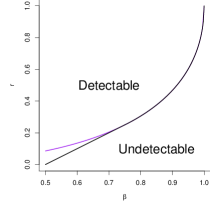
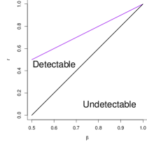
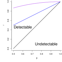
Then the curve in the plane is the detection boundary for this testing problem, in the sense that the LRT is asymptotically powerful (resp. powerless) when (resp. ). If , We call moderately sparse the regime where and very sparse the regime where . See Figure 1 for an illustration.
Following standard arguments, we extend these results to the dense regime, which we did not find elsewhere in the literature, except for the normal model (Cai et al., 2011).
Proposition 1.
Assume that and where . Then the hypotheses merge asymptotically when and , or when and
1.2 The higher criticism
Assuming known, Donoho and Jin (2004) proposed a procedure, called higher criticism, which does not require knowledge of , and is much simpler than the discretized generalized LRT proposed in (Ingster, 2002a, b), which still requires knowledge of . Among other things, they showed that, for any , the higher criticism is asymptotically optimal (i.e., achieves the detection boundary) in the sense that it is asymptotically powerful when . Inspired by an idea of John Tukey for multiple testing, this test is based on the normalized empirical process of the , and as such, is a special case of the goodness-of-fit test proposed by Anderson and Darling (1952). Specifically, the test rejects for large values of
| (9) |
where is the empirical distribution function.
Similar results have been obtained for other mixture models (e.g., chi-squared) in (Donoho and Jin, 2004; Jin, 2003); for a normal model where is standard normal and is normal with unknown variance (Cai et al., 2011); and also under dependence (Hall and Jin, 2008, 2010). More recently, Cai and Wu (2012) consider the detection problem in greater generality, but still assume that the null distribution is known. Focusing on the sparse regime where , they derive a detection boundary by characterizing the sharp asymptotics of the Hellinger distance between the null and the alternative, and then show that the higher criticism achieves the detection boundary, without knowledge of . We also mention the work of Jager and Wellner (2007), who propose a goodness-of-fit testing approach based on -divergences that includes the higher criticism as a special case. We stress the fact that all these works assume that the null distribution is known.
In the context of testing in a linear regression model with Gaussian noise, Ingster et al. (2010) and Arias-Castro et al. (2011) discuss the case where the noise variance is unknown, corresponding here to a situation where is known to be in a parametric family.
As far as we know, the only other publication that considers a nonparametric setting is (Delaigle et al., 2011), where the ’s are -statistics, for example obtained from the comparison of two samples as in some gene expression analysis; there, conditions are derived under which the higher criticism is asymptotically powerful as the degree of freedom of the -statistics tends to infinity.
1.3 A new testing procedure: the CUSUM sign test
Since is assumed to be symmetric (A1), it makes sense to test for symmetry. We prove in this paper that none of the classical procedures are completely satisfactory in that, in the context of the normal model (for example), they do not achieve the same asymptotic performance of the LRT in all regimes, and none of them achieves the detection boundary in the moderately sparse regime. We propose a new test for symmetry that is satisfactory in that sense.
To better explain the rationale behind our testing procedure, we draw a parallel with the higher criticism. In the normal model, the Kolmogorov-Smirnov test is suboptimal in the sparse regimes. This is because the deviations of the corresponding statistic
| (10) |
are dominated by what happens near the median of the distribution, since . Compare with the higher criticism (aka, Anderson-Darling) statistic (9), where each statistic in the supremum has unit variance.
The Kolmogorov-Smirnov test has an analogous test for symmetry, called the Smirnov test, based on
| (11) |
It can be seen as comparing the positive and negative parts of the sample; or as comparing with its symmetrization . The Smirnov statistic may be expressed as
| (12) |
in terms of the sign sequence
| (13) |
where are the observations sorted in decreasing order according their absolute value. This sign sequence is i.i.d. Rademacher under the null.
Our cumulative sum (CUSUM) sign test is to the Smirnov test for symmetry what the Anderson-Darling test is to the Kolmogorov-Smirnov test. It is based on
| (14) |
And indeed, under the null, for all .
1.4 Content
The remaining of the paper is organized as follows.
In Section 2, we analyze the CUSUM sign test, and another new test, that we named the tail-run test, based on the first run of 1’s in the sign sequence. We will show that the tail-run test is asymptotically optimal in the very sparse regime of the generalized Gaussian model. In fact, in our numerical experiments, the tail-run test outperforms the CUSUM sign test in that regime.
In Section 3, we analyze classical tests. In Section 3.1, we analyze the -test222When has finite variance, the -test is asymptotically distribution-free as a consequence of the Central Limit Theorem. and the sign test, considered as tests for the median. In Section 3.2, we analyze some emblematic tests for symmetry: the Wilcoxon signed-rank test, the Smirnov test, the number-of-runs test and the longest-run test. The study of these classical tests in the context of our testing problem (1)-(2) is novel as far as we know. We find that the -test, the sign test, the signed-rank test and the Smirnov test are all asymptotically optimal in the dense regime of the generalized Gaussian model, but grossly suboptimal in the sparse regime. We also find that the number-of-runs test is grossly suboptimal in all regimes, while the longest-run test is optimal for the generalized Gaussian model in the very sparse regime, but grossly suboptimal otherwise.
In Section 4, we perform numerical simulations to accompany our theoretical findings. We focus on the generalized Gaussian mixture model.
Section 5 is a short discussion section, where we contrasts our testing problem where all effects are positive to the analogous testing problem where the effects can be negative or positive in the same experiment.
1.5 Notation
For , let and . For , is the positive part. For two sequences of reals and : when ; when ; when is bounded; when and ; when . Finally, when for some .
We use similar notation with a superscript when the sequences and are random. For instance, means that is bounded in probability, i.e., as .
When and are random variables, means they have the same distribution. For a random variable and distribution , means that has distribution . For a sequence of random variables and a distribution , means that converges in distribution to . Everywhere, we identify a distribution and its cumulative distribution function. For a distribution , will denote its survival function.
2 New nonparametric tests for detecting heterogeneity
In this section, we study the CUSUM sign test and the tail-run test, respectively based on the statistics defined in (14) and (17).
2.1 The cumulative sum (CUSUM) sign test
We analyze the CUSUM sign test, which rejects for large values of defined in (14). Under the null, (Darling and Erdös, 1956).
Proposition 2.
Assuming (A1), the cumulative sums sign test is asymptotically powerful if either
| (15) |
or there is a sequence such that
| (16) |
Condition (15) is useful in the dense regime, where the CUSUM sign test behaves like the sign test (compare with (24)). In essence, the quantity on the LHS measures (in a standardized scale) how much the positive effects in (2) move the median away from 0. Condition (16) is useful in the sparse regime, where the quantity on the LHS measures how much of a ‘bump’ in the tail of the mixture distribution (2) the positive effects create.
Generalized Gaussian mixture model. We apply Proposition 2 when is generalized Gaussian with parameter as in Section 1.1. In the dense regime , we use the fact that
when , so that the CUSUM sign test achieves the detection boundary when . In the sparse regime , let as in (6). Note that, when , , where the density is defined in (4). We choose for some fixed chosen later on. We then have
and
where is defined in Section 1.5. Therefore, if denotes the LHS in (16), then
-
•
If , we choose , so that . In that case, when , we have
using the fact that .
-
•
If , we define . If , we choose , in which case
and when . If , we choose , yielding
Both exponents are positive when the first one is, which is the case when .
Comparing with the information bounds obtained by Donoho and Jin (2004) and described in Section 1.1, we see that the CUSUM sign test achieves the detection boundary for the generalized Gaussian mixture model.
2.2 The tail-run test
We now consider the tail-run test, which rejects for large values of
| (17) |
It is closely related to the trimmed longest run test of Baklizi (2007). We note that, under the null, since in that case the signs introduced in (13) are i.i.d. Rademacher random variables.
Proposition 3.
Assuming (A1), the tail-run test is asymptotically powerful if there exists a sequence such that
| (18) |
it is asymptotically powerless if there exists a sequence such that
| (19) |
Condition (18) says, in order, that the expected number of observations from that exceed tends to zero, that the expected number of observations from that are below tends to zero, and that the expected number of observations from that exceed tends to infinity. Clearly, this implies that the sign sequence starts with a number of pluses that diverges to infinity in probability, so that the test is asymptotically powerful. In contrast to that, Condition (19) implies that the first sign in the sign sequence will come from the sign of a null observation with probability tending to one, so that the test is asymptotically powerless.
We remark that, if in (18), then it implies (16), guaranteeing that the CUSUM sign test is asymptotically powerful. That said, in numerical experiments, the tail-run test clearly dominates the CUSUM sign test in the very sparse regime.
Generalized Gaussian mixture model. We apply Proposition 3 when is generalized Gaussian with parameter as in Section 1.1. We parameterize as in (6), namely, for some , and as always. Fix and choose . Using the fact that when , we have
| (20) |
When is fixed, we may choose small enough that the exponent in (20) is positive, implying that (18) holds. Comparing with the information bounds described in Section 1.1, we see that the tail-run test achieves the detection boundary in the very sparse regime when . Otherwise, it is suboptimal. In fact, based on (19), we find that the detection boundary for the tail-run test is given by
which is the same as that of the max test (based on ).
3 Classical tests
In this section we study some classical tests for the median, and also some classical tests for symmetry, which are both applicable in our context.
3.1 Tests for the median
Under mild assumptions on , for example if is strictly increasing at 0, the mixture distribution in (2) has strictly positive median, so that we may use a test for the median to test for heterogeneity. We study two such tests: the -test and the sign test.
3.1.1 The -test
Remember that the -test rejects for large values of
| (21) |
The distribution of under the null is scale-free and asymptotically standard normal for all with finite second moment. With that additional assumption, the -test is asymptotically distribution-free. (Below, we require finite fourth moments for technical reasons.)
Proposition 4.
Assume (A1), and that and have finite fourth moments. Then the -test is asymptotically powerful (resp. powerless) if
| (22) |
In particular, in the generalized Gaussian mixture model with parameter , the -test achieves the detection boundary in the dense regime if , and grossly suboptimal in the sparse regime(s), where it requires that increase at least polynomially in to be powerful.
3.1.2 The sign test
The sign test rejects for large values of
| (23) |
where the sign sequence is defined in (13). Under the null, , since in that case are i.i.d. Rademacher random variables.
Proposition 5.
Assuming (A1), the sign test is asymptotically powerful (resp. powerless) if
| (24) |
We first note that the sign test is asymptotically powerless when . We also note that, when is differentiable at 0 with strictly positive derivative,
| (25) |
Compare with (22). Otherwise, except for the term on the RHS, (24) coincides with (15), implying that, in the generalized Gaussian mixture model with parameter , the sign test achieves the detection boundary in the dense regime if .
3.2 Tests for symmetry
Assuming that is symmetric — a reasonable assumption in our nonparametric setting — places the problem in the context of testing for symmetry, which has been considerably discussed in the literature. Beyond the signed-rank test (Wilcoxon, 1945), many other methods have been proposed: there are tests based on runs statistics (Cohen and Menjoge, 1988; Baklizi, 2007); tests of Kolmogorov-Smirnov type (Smirnov, 1947) or Cramér - von Mises type (Rothman and Woodroofe, 1972; Aki, 1987; Cabaña and Cabaña, 2000; Einmahl and McKeague, 2003; Orlov, 1972); tests with bootstrap calibration (Schuster and Barker, 1987; Arcones and Giné, 1991); tests based on kernel density estimation (Ahmad and Li, 1997; Osmoukhina, 2001); tests based on trimmed Wilcoxon tests and on gaps (Antille et al., 1982); tests based on measures of skewness (Mira, 1999); and many more. We study a few emblematic tests for symmetry: the signed-rank test, the Smirnov test, the number-of-runs test and the longest-run test.
Recall the definition of the sign sequence in (13).
3.2.1 The signed-rank test
The Wilcoxon signed-rank test (Wilcoxon, 1945) rejects for large values of
| (26) |
Under the null, the distribution of is known in closed form, and is asymptotically standard normal (Hettmansperger, 1984).
Proposition 6.
Assume (A1), that and have densities and , and that
| (27) |
Then the signed-rank test is asymptotically powerful (resp. powerless) if
| (28) |
where and .
Condition (27) prevents from being skewed to the left, and makes and non-negative, since
| (29) | ||||
| (30) |
where the inequality comes from (27) and is an equality when is symmetric about 0. Similarly,
If is symmetric,
We first note that the signed-rank test is asymptotically powerless when since . (In fact, this is the case whether (27) holds or not.) For the rest of this discussion, assume that .
-
•
When is not symmetric, is bounded away from 0 since the first inequality in (30) is strict in that case. Hence, the signed-rank test is asymptotically powerful when .
- •
3.2.2 The Smirnov test
Recall the Smirnov test (Smirnov, 1947) based on the statistic defined in (11), or equivalently in (12). Under the null, is a simple symmetric random walk, so the reflection principle gives
In particular, is asymptotically distributed as the absolute value of the standard normal distribution.
Proposition 7.
Assuming (A1), the Smirnov test is asymptotically powerful (resp. powerless) if
| (31) |
We first note that the Smirnov test is asymptotically powerless when .
3.2.3 The number-of-runs test
The number-of-runs in the sign sequence is equal to , where
| (32) |
is the number of sign changes. For example, in the sequence
The number of runs test (Cohen and Menjoge, 1988; McWilliams, 1990) rejects for small values of . Under the null, , since the summands in (32) are i.i.d. Rademacher random variables in this case.
Here we content ourselves with a negative result showing that this test is comparatively less powerful than the other tests analyzed previously for testing heterogeneity.
Proposition 8.
Assume (A1), and that and have densities and that are positive everywhere. Then the number of runs test is asymptotically powerless if
| (33) |
where
| (34) |
and
| (35) |
We first note that , so the test is asymptotically powerless in the sparse regime .
We apply Proposition 8 when is generalized Gaussian with parameter . Assume that . Then . Indeed, define . Then
Hence, the test is asymptotically powerless if . This shows that, within this model, the test is much weaker than the sign test, the signed-rank test or the Smirnov test, which only require to be powerful.
3.2.4 The longest-run test
The length of the longest-run (of pluses) is defined as
| (36) |
For example, in the sequence
The longest-run test (Mosteller, 1941) rejects for large values of . The asymptotic distribution of under the null is sometimes called the Erdős-Rényi law, due to early work by Erdős and Rényi (1970), who discovered that almost surely. The limiting distribution was derived later on (Arratia et al., 1989).
Proposition 9.
Assume (A1), and that and have densities and that are positive everywhere. Then the longest-run test is asymptotically powerless if there is a sequence such that
| (37) |
and
| (38) |
It is asymptotically powerful if either:
-
(i)
There is a sequence such that
(39) -
(ii)
There is a sequence satisfying (37), another sequence with , as well as , and fixed, such that
(40) and
(41)
Of all the classical tests that we studied, this is the only one with some power in the sparse regime. The flip side is that it has very little power in the dense regime.
We apply Proposition 9 when is generalized Gaussian with parameter . Ignoring the term on the RHS, (39) is essentially equivalent to (18), and as a consequence, the longest-run test is asymptotically powerful when . However, this is not the detection boundary for the longest-run test in all cases. Indeed, assume that . Recall the parameterization of and in (5) and (6), where is fixed. Choose where is chosen below. Then using the fact that when , we have
for large enough. Let be such that . Then observe that, for fixed,
when . Choose sufficiently small that , so that (40) is satisfied with . Finally,
so that (41) is satisfied with . We conclude that the test is asymptotically powerful when . This can be seen to be sharp based on (37)-(38), so that the detection boundary for the longest run test is given by , meaning
4 Numerical experiments
In this section, we perform simple simulations to quantify the finite-sample performance of each of the tests whose theoretical performance we established. We consider the normal mixture model and some other generalized Gaussian mixture models.
In all these models, we take as benchmarks the likelihood ratio test (LRT) and the higher criticism (HC) — we used the variant recommended by Donoho and Jin (2004). The LRT is the optimal test when the models (1)-(2) are completely specified, meaning when are all known. The HC has strong asymptotic properties under various mixture models and only requires knowledge of . All the other tests we considered are distribution-free, except for the -test, which is only so asymptotically.
4.1 Fixed sample size
In this first set of experiments, the sample size was set at . In the alternative, instead of a true mixture as in (2), we drew exactly observations from and the other from . We did so to avoid important fluctuations in the number of positive effects, particularly in the very sparse regime. All models were parameterized as described in Section 1.1. In particular, with fixed, and in all cases, in the dense regime . We chose a few values for the parameter , illustrating all regimes pertaining to a given model, while the parameter (or ) took values in a finer grid. Each situation was repeated 200 times for each test. We calibrated the distribution-free tests, and the -test, using their corresponding limiting distributions under the null — which was accurate enough for our purposes since the sample size is fairly large — setting the level at 0.05. The LRT and HC were calibrated by simulation and set at the same level. What we report is the average empirical power — the fraction of times the alternative was rejected.
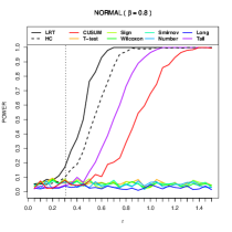
4.1.1 Normal mixture model
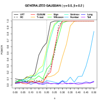
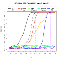
In this model, is standard normal. The simulation results are reported in Figure 2.
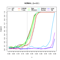
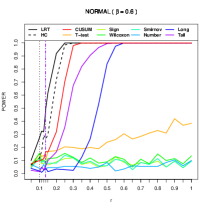
Dense regime. We set and with ranging from 0 to 0.5 with increments of 0.025. From Section 1.1, the detection threshold is at . Moreover, the results we established in Section 3 imply that the -test, sign, signed-rank, Smirnov tests, as well as our CUSUM sign test, all achieve this detection threshold. The simulations are clearly congruent with the theory, will all these tests closely matching the performance of the LRT, with the HC and CUSUM sign test lagging behind a little bit. We also saw that the number-of-runs test is asymptotically less powerful than the aforementioned tests, and that the longest-run and tail-run tests are essentially powerless in the dense regime. This is obvious in the power plots.
Moderately sparse regime. We set and with ranging from 0 to 1 with increments of 0.05, and added three more points equally spaced between 0.1 and 0.15 to zoom in on the phase transition. Our theory says that all distribution-free tests are asymptotically powerless, except for the longest-run, tail-run and CUSUM sign tests, with the latter outperforming the other two. This is indeed what happens in the simulations, although there is a fair amount of difference in power between the longest-run and tail-run tests. The CUSUM sign test lags a little behind the HC. The -test shows some power, although not much.
Very sparse regime. We set and with ranging from 0 to 1.5 with increments of 0.05. Our theory says that all distribution-free tests are asymptotically powerless, except for the longest-run, tail-run and CUSUM sign tests, and that all three are asymptotically near-optimal. In the simulations, however, the longest-run test shows no power whatsoever, and the tail-run test is noticeably more powerful than the CUSUM sign test, although quite far from the performance of the HC, which almost matches that of the LRT. To understand what is happening, take the most favorable situation for the tail-run test, where all positives effects — 16 of them here — are larger than all the other observations in absolute value. In that case, the tail-run is of length , resulting in a p-value for that test smaller than . For the CUSUM sign test, . But under the null, is close to , with deviations of about (obtained from simulations). So even then, the number of true positives is barely enough to allow the CUSUM sign test to be fully powerful. As for the longest-run test, under the null, the longest-run is of length about , with deviations of about , which explains why this test has no power.
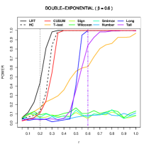
4.1.2 Double-exponential mixture model
In this model, is double-side exponential with variance 1. The simulation results are reported in Figure 3.
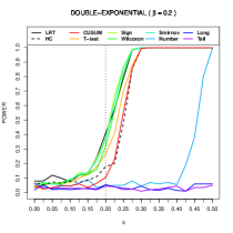
Dense regime. The setting is exactly as in the normal mixture model. Our theoretical findings were also similar, and are corroborated by the simulations.
Sparse regime. We set and with ranging from 0 to 1 with increments of 0.05. The simulations are congruent with the theory, with the CUSUM sign test and HC being close in performance, while the longest-run and tail-run tests are far behind as predicted by the theory. The -test shows a fair amount of power here, and is even fully powerful at . The other tests are powerless as predicted by the theory.
4.1.3 Generalized Gaussian mixture model with
In this model, is generalized Gaussian with parameter . The simulation results are reported in Figure 4.
Dense regime. The setting is exactly as in the normal mixture model. Our theoretical findings were also similar. The simulations illustrate the theory fairly well, although in this finite-sample situation we observe that the spread in performance is wider than before, with the best performing tests being the sign and Smirnov tests — not far from the reigning LRT — ahead of the signed-rank and CUSUM sign tests, very close to the HC, and then comes the -test and number-of-runs test quite far behind. The other two tests have no power.
Sparse regime. We set and with ranging from 0 to 1 with increments of 0.05. The CUSUM sign test is slightly inferior to the HC, far above the longest-run test, as predicted by our theory. The tail-run test has no power here, although the theory says it should have some at . The -test, surprisingly, dominates the longest-run test.
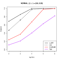
4.2 Varying sample size
In this second set of experiments, we examined various sample sizes to assess the effect of smaller sample sizes on the power of the distribution-free tests in particular. We focused on the CUSUM sign test and tail-run test, comparing them with the LRT and HC in the normal mixture model. The simulation results are reported in Figure 5.
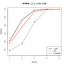
Dense regime. We fixed , and chose , as sample sizes, with number of positives 40, 251, 1585, , 63096 respectively. We see that, for all test, the power increases rapidly with the sample size.
Sparse regimes. For the moderately sparse regime, we fixed , and chose , , with number of positives , respectively. For the very sparse regime, we fixed , and chose , , with number of positives , respectively. In both cases, the CUSUM sign and the tail-run tests are more affected by the small sample sizes than the LRT or HC.
5 Discussion
5.1 Beyond the generalized Gaussian mixture model
Although we used the generalized Gaussian mixture model as a benchmark for gaging the performance of the various tests studied here, this can be done in much more generality. Assume for simplicity.
-
•
For the dense regime, if differentiable and satisfies the conditions of Proposition A.1, then all tests are asymptotically powerless when . On the other hand, if is differentiable at 0 with , then the CUSUM sign, -, sign, signed-rank and Smirnov tests are all asymptotically powerful when .
-
•
For the sparse regime, all the results apply in the same way if instead of a strict generalized Gaussian distribution (4) we have and
In particular, the CUSUM sign test achieves the detection boundary in all these models, simultaneously.
5.2 Positive and negative effects
A crucial assumption is that all the effects have same sign (here assumed positive). When the effects can be negative or positive in the same experiment, then the problem is very different, as the assumption that is symmetric does not really help, since now the contamination can also be symmetric. This is for instance the case in the canonical model:
It is known that the detection boundary remains the same for generalized Gaussian mixture models in the sparse regime, and that the higher criticism remains near-optimal. However, we do not know how to design a near-optimal distribution-free test in such a situation. Perhaps there is no distribution-free test that matches the performance of the higher criticism.
Acknowledgements
We would like to thank Jason Schweinsberg for helpful discussions. This work was partially supported by a grant from the Office of Naval Research (N00014-09-1-0258).
References
- Ahmad and Li (1997) Ahmad, I. A. and Q. Li (1997). Testing symmetry of an unknown density function by kernel method. J. Nonparametr. Statist. 7(3), 279–293.
- Aki (1987) Aki, S. (1987). On nonparametric tests for symmetry. Ann. Inst. Statist. Math. 39(3), 457–472.
- Anderson and Darling (1952) Anderson, T. W. and D. A. Darling (1952). Asymptotic theory of certain “goodness of fit” criteria based on stochastic processes. Ann. Math. Statistics 23, 193–212.
- Antille et al. (1982) Antille, A., G. Kersting, and W. Zucchini (1982). Testing symmetry. J. Amer. Statist. Assoc. 77(379), 639–646.
- Arcones and Giné (1991) Arcones, M. A. and E. Giné (1991). Some bootstrap tests of symmetry for univariate continuous distributions. Ann. Statist. 19(3), 1496–1511.
- Arias-Castro et al. (2011) Arias-Castro, E., E. J. Candès, and Y. Plan (2011). Global testing under sparse alternatives: Anova, multiple comparisons and the higher criticism. Ann. Statist.. To appear.
- Arratia et al. (1989) Arratia, R., L. Goldstein, and L. Gordon (1989). Two moments suffice for Poisson approximations: the Chen-Stein method. Ann. Probab. 17(1), 9–25.
- Baklizi (2007) Baklizi, A. (2007). Testing symmetry using a trimmed longest run statistic. Aust. N. Z. J. Stat. 49(4), 339–347.
- Berk (1973) Berk, K. N. (1973). A central limit theorem for -dependent random variables with unbounded . Ann. Probability 1, 352–354.
- Cabaña and Cabaña (2000) Cabaña, A. and E. M. Cabaña (2000). Tests of symmetry based on transformed empirical processes. Canad. J. Statist. 28(4), 829–839.
- Cai et al. (2011) Cai, T. T., X. J. Jeng, and J. Jin (2011). Optimal detection of heterogeneous and heteroscedastic mixtures. J. R. Stat. Soc. Ser. B Stat. Methodol. 73(5), 629–662.
- Cai and Wu (2012) Cai, T. T. and Y. Wu (2012). Optimal detection for sparse mixtures. Available online http://arxiv.org/abs/1211.2265.
- Cohen and Menjoge (1988) Cohen, J. P. and S. S. Menjoge (1988). One-sample run tests of symmetry. J. Statist. Plann. Inference 18(1), 93–100.
- Darling and Erdös (1956) Darling, D. A. and P. Erdös (1956). A limit theorem for the maximum of normalized sums of independent random variables. Duke Math. J. 23, 143–155.
- Delaigle et al. (2011) Delaigle, A., P. Hall, and J. Jin (2011). Robustness and accuracy of methods for high dimensional data analysis based on Student’s -statistic. J. R. Stat. Soc. Ser. B Stat. Methodol. 73(3), 283–301.
- Donoho and Jin (2004) Donoho, D. and J. Jin (2004). Higher criticism for detecting sparse heterogeneous mixtures. Ann. Statist. 32(3), 962–994.
- Einmahl and McKeague (2003) Einmahl, J. H. J. and I. W. McKeague (2003). Empirical likelihood based hypothesis testing. Bernoulli 9(2), 267–290.
- Erdős and Rényi (1970) Erdős, P. and A. Rényi (1970). On a new law of large numbers. J. Analyse Math. 23, 103–111.
- Hall and Jin (2008) Hall, P. and J. Jin (2008). Properties of higher criticism under strong dependence. Ann. Statist. 36(1), 381–402.
- Hall and Jin (2010) Hall, P. and J. Jin (2010). Innovated higher criticism for detecting sparse signals in correlated noise. Ann. Statist. 38(3), 1686–1732.
- Hettmansperger (1984) Hettmansperger, T. P. (1984). Statistical inference based on ranks. Wiley Series in Probability and Mathematical Statistics: Probability and Mathematical Statistics. New York: John Wiley & Sons, Inc.
- Ingster et al. (2010) Ingster, Y., A. Tsybakov, and N. Verzelen (2010). Detection boundary in sparse regression. Electronic Journal of Statistics 4, 1476–1526.
- Ingster (1997) Ingster, Y. I. (1997). Some problems of hypothesis testing leading to infinitely divisible distributions. Math. Methods Statist. 6(1), 47–69.
- Ingster (2002a) Ingster, Y. I. (2002a). Adaptive detection of a signal of growing dimension i. Math. Methods Statist. 10, 395–421.
- Ingster (2002b) Ingster, Y. I. (2002b). Adaptive detection of a signal of growing dimension ii. Math. Methods Statist. 11, 37–68.
- Jager and Wellner (2007) Jager, L. and J. Wellner (2007). Goodness-of-fit tests via phi-divergences. Ann. Statist. 35(5), 2018—2053.
- Jennen-Steinmetz and Gasser (1986) Jennen-Steinmetz, C. and T. Gasser (1986). The asymptotic power of runs tests. Scand. J. Statist. 13(4), 263–269.
- Jin (2003) Jin, J. (2003). Detecting and Estimating Sparse Mixtures. Ph. D. thesis, Stanford University.
- Lehmann and Romano (2005) Lehmann, E. L. and J. P. Romano (2005). Testing statistical hypotheses (Third ed.). Springer Texts in Statistics. New York: Springer.
- McWilliams (1990) McWilliams, T. P. (1990). A distribution-free test for symmetry based on a runs statistic. J. Amer. Statist. Assoc. 85(412), 1130–1133.
- Mira (1999) Mira, A. (1999). Distribution-free test for symmetry based on Bonferroni’s measure. J. Appl. Statist. 26(8), 959–972.
- Mosteller (1941) Mosteller, F. (1941). Note on an application of runs to quality control charts. Ann. Math. Statistics 12, 228–232.
- Orlov (1972) Orlov, A. I. (1972). Testing the symmetry of a distribution. Teor. Verojatnost. i Primemen. 17, 372–377.
- Osmoukhina (2001) Osmoukhina, A. V. (2001). Large deviations probabilities for a test of symmetry based on kernel density estimator. Statist. Probab. Lett. 54(4), 363–371.
- Rothman and Woodroofe (1972) Rothman, E. D. and M. Woodroofe (1972). A Cramér-von Mises type statistic for testing symmetry. Ann. Math. Statist. 43, 2035–2038.
- Schuster and Barker (1987) Schuster, E. F. and R. C. Barker (1987). Using the bootstrap in testing symmetry versus asymmetry. Comm. Statist. B—Simulation Comput. 16(1), 69–84.
- Smirnov (1947) Smirnov, N. V. (1947). Sur un critère de symétrie de la loi de distribution d’une variable aléatoire. C. R. (Doklady) Acad. Sci. URSS (N.S.) 56, 11–14.
- Wald and Wolfowitz (1940) Wald, A. and J. Wolfowitz (1940). On a test whether two samples are from the same population. Ann. Math. Statistics 11, 147–162.
- Wilcoxon (1945) Wilcoxon, F. (1945). Individual comparisons by ranking methods. Biometrics Bulletin 1(6), 80–83.
Appendix A Lower bounds
We let and denote the probability, expectation and variance under the null and alternative, respectively.
A.1 Truncated moment method
Ingster (1997) devised a general method for showing that the LRT (and therefore any other test) is asymptotically powerless. It is based on the first two moments of a truncated likelihood ratio. It yields the following.
Lemma A.1.
Let and denote the densities of and with respect to a dominating measure. Then the hypotheses merge asymptotically when there is a sequence such that
| (A.1) |
and
| (A.2) |
Proof.
The likelihood ratio is given by
The test minimizes the risk at
where for any . (Note that is the total variation distance between and .) We do not work with directly, but truncate it first. Define
Using the fact that and then the Cauchy-Schwarz inequality, we have
And since
to prove that , it suffices that
A.2 Proof of Proposition 1
We may assume that . We have
where . When , , so that
When , we have
Hence,
We used dominated convergence in the last line. Hence, by Lemma A.1 (with ), the hypotheses merge asymptotically when . When , when . When , when . When , when .
We now show that the hypotheses separate completely when and , or when and . We will show later that several tests (CUSUM, t, sign, signed-rank, Smirnov) are asymptotically powerful in this setting in the former situation, so we focus on the latter. For this, it suffices to do as Cai and Wu (2012), and show that
where denote the Hellinger distance. When , we have Hence,
The result comes from that.
A.3 A general information bound for the dense regime
The following result does not require symmetry. Note that below are implicitly known.
Proposition A.1.
Assume that . When , then there is a test that asymptotically separates and . When , assume that is symmetric about 0 and has a differentiable density that satisfies for all and all , with
Then the hypotheses are asymptotically inseparable if
Compare with the performance bounds obtained for the CUSUM sign test, the -test, the sign test, signed-rank test, and the Smirnov test, which were shown to be asymptotically powerful when under mild additional conditions. Note that Proposition A.1 is strong enough to imply Proposition 1 when .
Proof.
First assume that . Extracting a subsequence if needed, we may assume that for some . If , then consider the test that rejects when is too large. We have
and using the fact that has zero median,
Therefore,
and we conclude with Lemma B.2 that there is a test based on that is asymptotically powerful. If , let be a measurable subset of such that . This is possible since . (If , this comes from the fact that while .) We then consider the test based on and reason as above. We have
and , so that
We now assume that . We first note that is integrable since, by the Cauchy-Schwarz inequality,
Then, because is even, is odd, and therefore . We have
with, by the Cauchy-Schwarz inequality,
and
Hence,
and we conclude with Lemma A.1 (with ). ∎
A.4 Generalized Gaussian mixture model (different parameters)
Suppose and are generalized Gaussian with parameters . By Proposition A.1, in the dense regime the two hypotheses and are asymptotically separable, so we focus on the sparse regime where with .
Case . Here, has heavy tails compared to , so much so that the max test — which rejects for large values of — is asymptotically powerful as soon as , even if . Indeed, with high probability under the null, , while under the alternative (with ), at least points are sampled from , and the maximum of them exceeds .
Case . Here, has lighter tails than , and as a consequence, the max test has very little power. This situation is more interesting. Following standard lines, we obtain the following.
Proposition A.2.
This coincides with the detection boundary when is generalized Gaussian with exponent . We note that the result is sharp. For example, the CUSUM sign test achieves this detection boundary. (We invite the reader to verify this based on Proposition 2.)
Proof.
We want to apply Lemma A.1. The first condition in (A.1) holds when , while the second condition in (A.1) is fulfilled when . Hence, the choice is valid.
We now turn to (A.2), where , with . For , we have
because . We therefore focus . We see that is increasing over and decreasing over , where be the (unique) root of over , specifically, satisfies . Expressing as for some , we have
Since , we necessarily have and thus . Hence, we have
leading to
when . ∎
Appendix B Performance bounds
We let , and denote the probability, expectation and variance under the mixture model (2). The corresponding notation for the null distribution (1) — corresponding to (2) with — is , and .
B.1 Proof of Proposition 2
By (Darling and Erdös, 1956), under the null, . Define , so that , as .
B.2 Proof of Proposition 3
We first show that the tail-run test is asymptotically powerful when (18) holds. Since under the null, it suffices to show that under the alternative. We first note that
by the union bound, the first two conditions in (18) and the fact that is symmetric. Therefore, with high probability. Now, where , so that , since by the third condition in (18).
Next, we show that the test is asymptotically powerless when (19) holds. For this, we need to show that is asymptotically stochastically bounded by . We do so by showing that , where is the length of the tail-run ignoring the true positive effects. (Note that .) Under the alternative, may be generated as follows. First, let be i.i.d. Bernoulli with mean , and then draw from (resp. ) if (resp. 1). Let and . By the second condition in (19), we have with probability tending to one. Assume this is the case. Let and . These are binomial random variables with by the first condition in (18), so that by Chebyshev’s inequality. So, with high probability, there is an observation such that , which therefore bounds the largest positive effect. In that case, is bounded by the length of the tail-run of positive signs in , which is equal to . We conclude that, indeed, with probability tending to one.
B.3 Moment method for analyzing a test
We state and prove a general result for analyzing a test. It is particularly useful when the corresponding test statistic is asymptotically normal both under the null and alternative hypotheses.
Lemma B.2.
Consider a test that rejects for large values of a statistic with finite second moment, both under the null and alternative hypotheses. Then the test that rejects when is asymptotically powerful if
| (B.1) |
Assume in addition that is asymptotically normal, both under the null and alternative hypotheses. Then the test is asymptotically powerless if
| (B.2) |
Proof.
Assume that is large enough that . By Chebyshev’s inequality, the test has a level tending to zero, that is, . Now assume we are under the alternative. Since
by Chebyshev’s inequality, we see that . Hence, this test is asymptotically powerful.
For the second part, we have
while
by Slutsky’s theorem, since and (B.2) holds. Hence, has the same asymptotic distribution under the two hypotheses, and consequently, is powerless at separating them. This immediately implies that any test based on is asymptotically powerless. ∎
B.4 Proof of Proposition 4
Redefining as , we may assume that without loss of generality. Define the sample mean and sample variance
so that . Under the null, are i.i.d. with distribution , which has finite second moment by assumption. Hence, the central limit theorem applies and is asymptotically normal with mean 0 and variance . Also,
by the law of large numbers. Hence, by Slutsky’s theorem, is asymptotically standard normal under the null.
We now look at the behavior of under the alternative. The ’s are still i.i.d., with and
| (B.3) |
Hence, by Chebyshev’s inequality,
using the fact that . Let , which are i.i.d. with and . For , we have
From this, it easily follows that . Since , we have and
so that
| (B.4) |
Hence, by Chebyshev’s inequality,
| (B.5) | ||||
using the fact that . Consequently,
When , we have
so that the test has vanishing risk.
The same arguments show that remains bounded when is bounded — implying that is bounded — in which case the -test is not powerful. To prove that the -test is actually powerless when requires showing that is also asymptotically standard normal in this case. By the fact that and , we have and also . Hence, from (B.3) we get , and from (B.4) we get . Therefore, on the one hand, by (B.5). On the other hand, Lyapunov’s conditions are satisfied for , since they are i.i.d. with and . Hence,
is asymptotically normal with mean 0 and variance . We conclude that is also asymptotically standard normal under the alternative when .
B.5 Proof of Proposition 5
The proof is a simple application of Lemma B.2. We work with , which is equivalent since . Note that
| (B.6) |
We have
and
Hence
provided . By Lemma B.2, this proves that the sign test is asymptotically powerful.
To prove that the test is powerless when the limit in (24) is 0, we first show that is asymptotically standard normal both under the null and under the alternative. The very classical normal approximation to the binomial says that
Under the alternative, we apply Lyapunov’s CLT. The condition are easily verified: since , and the variables we are summing — here — are bounded. Hence, it follows that is asymptotically standard normal. And it is easy to see that condition (B.2) holds when . By Lemma B.2, this proves that the sign test is asymptotically powerless.
B.6 Proof of Proposition 6
The proof is based on Lemma B.2. We work with , which is equivalent since . The first and second moments of are known in closed form and, when the distribution of the variables is fixed, it is known to be asymptotically normal (Hettmansperger, 1984). For completeness, and also because the distribution under the alternative changes with the sample size, we detail the proof, although no new argument is needed.
The crucial step is to represent as a U-statistic:
This facilitates the computation of moments, and also the derivation of the asymptotic normality.
Define , , and . We have
and
Under the alternative, the ’s are i.i.d. with distribution and density . We get
and
using the fact that is even and the following identities:
and
Similarly, we compute
and
Substituting the parameters in the formulas, we obtain
| (B.7) |
with , and
| (B.8) |
In particular,
and .
Therefore, when , the test that rejects for large values of is asymptotically powerful by Lemma B.2. We also note that (B.2) is satisfied when , so it remains to show that is asymptotically normal. (It is well-known that is asymptotically normal under the null.) We follow the footsteps of Hettmansperger (1984). We quickly note that , which is negligible compared to the standard deviation of , which is of order . So it suffices to show that is asymptotically normal. Its Haj́ek projector is
and satisfies and . It is easy to see that
so that
Hence, since the variables are bounded, Lyapunov conditions are satisfied and is asymptotically normal. Coming back to , we have , so that
and therefore
We conclude that is asymptotically normal also.
B.7 Proof of Proposition 7
We work with the form (11), meaning we consider the test that rejects for large values of , where for a distribution function , with .
We already know that under the null hypothesis.
Define and as in the proof of Proposition 3. Let and for . We have , so that
By the triangle inequality,
| (B.9) |
and also
| (B.10) |
For the null effects in the sample, because is symmetric and , we have . For the true positive effects in the sample, by the triangle inequality,
| (B.11) | |||
To see why the term on the RHS is bounded, we note that, given ,
where denotes the empirical distribution function of an i.i.d. sample of size drawn from and denotes the maximum absolute value of a Brownian bridge over . ( here means “distributed as”.) Since , we infer that the same weak convergence holds unconditionally.
We now prove that the test is asymptotically powerful when the limit in (31) is infinite. Under the alternative, by (B.11) plugged into (B.9), we get
where the divergence to is due to (31) diverging and the fact that . Since under the null, we conclude that the test is indeed powerful.
Next, we show that the test is asymptotically powerless when the limit in (31) is zero. By (B.11) plugged into (B.9), we get
using the fact that and , combined with (31) converging to zero. Hence, under the alternative, which is the same limiting distribution as under the null. We conclude that the test is asymptotically powerless.
B.8 Proof of Proposition 8
We note that our proof relies on different arguments than those of Cohen and Menjoge (1988), which are based on the classical work of Wald and Wolfowitz (1940). Instead, we use a Central Limit Theorem for -dependent processes due to Berk (1973). We also mention Jennen-Steinmetz and Gasser (1986), who tests whether independent Bernoulli random variables have the same parameter, or not.
For , define
Let and . Note that in the denominator in is the density of in model (2). Given , the signs are independent Bernoulli with parameters , where and are the ordered ’s. We mention that the ’s are generally not unconditionally independent.
To prove powerlessness, we use the fact that is asymptotically normal under both hypotheses and then apply Lemma B.2. Under the null, we saw that , and asymptotic normality comes from the classical CLT.
Let
Noting that when is large enough that , we have by (33). It therefore exists such that . Define as the set of , such that
| (B.12) |
Note that , where and is drawn from the mixture model (2). Also, for all . Hence, letting , we have
using the fact that in the first and third inequalities, and the second is Bernstein’s inequality together with the fact that , since . Hence, using the fact that , we conclude that
So it suffices to work given . Let denote the distribution of under model (2) given , where .
Let , so that . Note that forms an -dependent process with . We apply the CLT of Berk (1973) to that process. We have . Then, due to the fact that given the ’s are independent, for we have
where
and
Put and note that . We have
and
so that
We also have
using the identity and (B.12) in the last inequality. Hence,
Thus the CLT of Berk (1973) applies to give that is also asymptotically normal under , along any sequence . Moreover, we also have . For the expectation, we have
and since , we have
So by Lemma B.2, the test that rejects for small values of is asymptotically powerless.
B.9 Proof of Proposition 9
We keep the same notation as in the previous section, except we redefine as the set of such that . Equivalently, .
We first prove that the test is asymptotically powerless under (37)-(38). First, by the union bound,
because of (37). Therefore, we work given as before.
Let and note that
When , we have that for all .
Let denote the length of the longest-run in a sequence of i.i.d. Bernoulli random variables with parameter . Also, let have the distribution . From (Arratia et al., 1989, Ex. 3), we have the weak convergence
when along a sequence such that .
Now, under the null, has the distribution of . Under , is stochastically bounded by . In fact, is itself stochastically bounded by in the limit. Indeed, on the one hand, we have
by (38); on the other hand, is stochastically bounded by , which converges to in distribution. We therefore conclude that the test is asymptotically powerless.
We now prove the asymptotic powerfulness of the test under either (39), or (40)-(41). In Case (i), we quickly note that (39) is identical to (18) except for the log factor in the rightmost condition, and the exact same arguments showing that the tail-run test is asymptotically powerful under (18) imply that, under (39), , where is the tail run defined in (17). Hence, under the alternative, , compared to under the null.
In Case , (37) holds, so that we may work given as before, and the arguments are almost the same as when we proved powerlessness, but in reverse. Let . Redefine and note that
as soon as . In fact, by (40), so that .
We have that , where is the longest-run of pluses among . The number of ’s falling in , denoted by , is stochastically larger than , where
where the last inequality holds eventually due to (41). Therefore, with high probability as , . Given this is the case, is stochastically bounded from below by , and we know that
We compare this with the size of under the null, which is :
since the constant factor is positive by the upper bound on .