Effective field theory as a limit of $R$-matrix theory for light nuclear reactions

Abstract

We study the zero channel radius limit of Wigner’s $R$-matrix theory for two cases, and show that it corresponds to non-relativistic effective quantum field theory. We begin with the simple problem of single-channel $np$ elastic scattering in the ${}^{1}\!S_{0}$ channel. The dependence of the $R$ matrix width $g^{2}$ and level energy $E_{\lambda}$ on the channel radius $a$ for fixed scattering length $a_{0}$ and effective range $r_{0}$ is determined. It is shown that these quantities have a simple pole for a critical value of the channel radius, $a_{p}=a_{p}(a_{0},r_{0})$. The ³H$(d,n)^{4}$He reaction cross section, analyzed with a two-channel effective field theory in the previous paper, is then examined using a two-channel, single-level $R$-matrix parameterization. The resulting $S$ matrix is shown to be identical in these two representations in the limit that $R$-matrix channel radii are taken to zero. This equivalence is established by giving the relationship between the low-energy constants of the effective field theory (couplings $g_{c}$ and mass $m_{*}$) and the $R$-matrix parameters (reduced width amplitudes $\gamma_{c}$ and level energy $E_{\lambda}$). An excellent three-parameter fit to the observed astrophysical factor $\overline{S}$ is found for ‘unphysical’ values of the reduced widths, $\gamma_{c}^{2}<0$.

I Introduction

In the previous companion paper BH13 , a two-channel effective quantum field theory (EFT) expression for the ³H$(d,n)^{4}$He reaction cross section at low energies was derived. It gives a very good description of the experimental data over the resonance region using only three parameters. In this paper, we examine its relation to the $R$-matrix theory, in the limit where the channel radii are taken to vanish.

We first consider the simpler problem of elastic $np$ scattering in the ${}^{1}\!S_{0}$ channel; it is free of any bound state and can be treated with a single channel $R$ matrix. This preliminary $np$ study provides insight into the channel radius dependence of the single-channel $R$ matrix parameters.

The main focus of this study is a two-channel, single-level $R$-matrix description of the ³H$(d,n)^{4}$He cross section, which is dominated by an ⁵He resonant contribution. We consider such a description both for the case of finite channel radii and in the limit as the channel radii approach zero. We find, as have others Resler92 ; Karnakov90 ; Karnakov91 , that an excellent fit to the experimental reaction data can be obtained with a single $R$-matrix level using channel radii that are on the order of the range of nuclear forces. This is consistent with the usual interpretation that the channel radii represent, in a qualitative sense, the short but non-zero range over which these forces act. It may then be somewhat surprising, however, that the high quality of the fit to the data is maintained with much smaller radii. Indeed, the excellent agreement persists for channel radii of zero if the square of the reduced widths are allowed to become (unphysically) negative. Remarkably, in this limit the $R$-matrix expression reduces identically to that determined in the EFT approach.

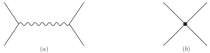
Given that the channel radii are associated with the range of the nuclear force, this identity establishes that the $R$-matrix description can be applied to theories with local couplings, as in Fig. 1a (to be contrasted with the contact coupling of Fig. 1b). The channel radii dependence of the $R$-matrix parameters, as the size of the interior region vanishes, gives insight into how the Lagrangian of the EFT description becomes “unphysical.”

Figure 1: Local (a) and contact (b) interaction mechanisms in the effective field theory approach. The equivalence of the zero channel radius $R$-matrix description, discussed in the text, to the EFT of Ref.BH13 demonstrates that it may be applied to theories with local interactions. Note that these statements should not be confused with those relating to theories with a contact interaction, as in (b).

The low-energy $np$ scattering is treated in Section II as a simple example, which may be expressed analytically, to obtain insight into the channel-radius dependence of the $R$-matrix parameters. In this case, the physical values of the ${}^{1}\!S_{0}$ scattering length and effective range are given by real $R$-matrix parameters at radii down to a critical channel radius of $a_{p}\simeq 1.30$ fm, but below that radius (and continuing to zero radius) the reduced-width amplitude $\gamma$ becomes pure imaginary, with $\gamma^{2}<0$.

In Section III we discuss the main result of the current study, a two-channel, single-level formula for the total ³H$(d,n)^{4}$He reaction cross section. We describe, in Subsection III.1, its application to the description of the reaction at finite channel radii with a four parameter fit. The derivation of a dispersion relation for the logarithmic derivative of the external outgoing-wave solution that is relevant to this development and, to our knowledge previously unpublished, is given in the Appendix. We then describe the dependence of the parameters of the fit on variations in the channel radii. In Subsection III.2 we show how the zero-radius limit of the $R$-matrix expression reduces to the one given by EFT in the companion paper.

Finally, we discuss the implications of our work and give conclusions in Section IV. The notation has been changed somewhat from the previous paper to correspond with that used more commonly in the $R$-matrix literature for nuclear reactions. For example, the channel labels will be shortened so that $d$ means $dt$ (or $d+^{3}$H) and $n$ stands for $n\alpha$ (or $n+^{4}$He). Other notational differences will be indicated as needed.

II Single-level Effective Range Expansion for $np$ Scattering

We investigate the dependence of the $R$-matrix parameters on the channel radius $a$, in limit that $a\to 0$ for a simple example: single-channel scattering in a neutral $S$-wave such as neutron-proton scattering.

We assume that the low-energy scattering is described by a single-level $R$-matrix

$$R(E;a)=\frac{\gamma^{2}(a)}{E_{\lambda}(a)-E}\,,$$ (1)

for which the scattering matrix is

$$e^{2i\delta_{0}(E)}=e^{-2ika}\frac{1+ika\,R(E;a)}{1-ika\,R(E;a)}\,,$$ (2)

where $k=\sqrt{2\mu E}/\hbar$ is the wave number in the center-of-mass, $\mu$ the reduced mass of the scattering pair, and $E_{\lambda}$ the energy eigenvalue of the level. Instead of the reduced width amplitude $\gamma$, we shall use $g^{2}=a\,\gamma^{2}$ because $g^{2}$ remains finite in the zero channel radius limit, $a\to 0$.

If we simply take the channel radius to vanish, $a\to 0$, then the transition amplitude becomes

$$i(e^{2i\delta_{0}(E)}-1)=2\frac{g^{2}k}{E-E_{\lambda}+ig^{2}k}\,.$$ (3)

This is proportional to the transition amplitude in the non-relativistic effective quantum field theory for two particles interacting via a single scalar intermediate field with energy $E_{\lambda}$. The zero of the energy scale, $E=0$, corresponds to vanishing relative motion of the scattering particles. In this field theory context, $g$ is, up to a conventional overall factor, the coupling constant of the scattering particles interacting with the intermediate field. The scattering amplitude (3) can be rewritten

$$k\cot\delta_{0}(E)=\frac{1}{g^{2}}\left(E_{\lambda}-E\right)\,.$$ (4)

This is precisely the effective range expansion

$$k\cot\delta_{0}(E)=-\frac{1}{a_{0}}+\frac{1}{2}r_{0}k^{2}\,,$$ (5)

with the identifications

$$a_{0}=-\frac{g^{2}}{E_{\lambda}}$$ (6)

for the scattering length, and

$$r_{0}=-\frac{\hbar^{2}}{g^{2}\mu}$$ (7)

for the effective range. The two-term effective range approximation for $k\cot\delta_{0}(E)$ is exact in this case.

We may, in general, have a low-energy cross section that results in either a positive or negative scattering length. Equations (6) and (7) demonstrate that, in the zero channel-radius limit, $a\to 0$, the sign of the $a_{0}$ is determined by whether the $R$-matrix parameters, $E_{\lambda}$ and $g^{2}$, of like ($a_{0}<0$) or differing ($a_{0}>0$) sign.

Turning to the effective range, $r_{0}$ we see that for a real coupling strength $g$, the effective range parameter is necessarily negative, $r_{0}<0$, independent of the sign of $E_{\lambda}$. A positive effective range, which is the predominant situation – as in ${}^{1}\!S_{0}$ neutron-proton scattering – may be obtained by the formal device of taking the coupling strength to be purely imaginary, $g\to ig$. Although this results in a structure that is unphysical from both the field-theoretic and $R$-matrix perspectives, it is an acceptable procedure for our limited objective of obtaining a low-energy description. In particular, the transition amplitude, Eq.(3) continues to satisfy unitarity under this transformation, which is equivalent to $g^{2}\to-g^{2}$. It is clear from Eq. (3) that the change $g^{2}\to-g^{2}$ is also equivalent to $\left(E-E_{\lambda}\right)\to\left(E_{\lambda}-E\right)$. In the field theory description, this is a transformation that changes the sign of the intermediate field’s unperturbed (free-field) propagator which is brought about by changing the sign of the intermediate field’s free Lagrangian. It is conventional, in work that applies effective quantum field theory to nuclear physics problems EHM09 , to employ the convention that the sign of the free-field intermediate Lagrangian is used with a “wrong sign” to obtain a positive effective range parameter, and so this is the convention used in our preceding paper BH13 . However, in our work here, it proves convenient to use the equivalent method of using an imaginary coupling constant.

We now wish to examine the $a$ dependence in detail and, in particular, the character of the $a\to 0$ limit. We return to the general $R$-matrix expression (2) with $a\neq 0$, which may be written as

$$k\cot\delta_{0}(E)=\frac{E_{\lambda}-\frac{\hbar^{2}k^{2}}{2\mu}+kg^{2}\tan ka}{g^{2}-(E_{\lambda}-\frac{\hbar^{2}k^{2}}{2\mu})\frac{1}{k}\tan ka}.$$ (8)

This gives the scattering length

$$a_{0}=a-\frac{g^{2}}{E_{\lambda}}\,,$$ (9)

and the effective range

$$r_{0}=\frac{2a^{3}E_{\lambda}^{2}/3-2a^{2}E_{\lambda}g^{2}+2ag^{4}-g^{2}\hbar^{2}/\mu}{(g^{2}-aE_{\lambda})^{2}}\,.$$ (10)

We study $g^{2}$ and $E_{\lambda}$ as functions of $a$ for fixed values of $a_{0}$ and $r_{0}$. To this end, we use the condition $g^{2}/E_{\lambda}=a-a_{0}$ from Eq. (9) in Eq. (10) to obtain

$$\frac{1}{2}r_{0}a_{0}^{2}=\frac{1}{3}a^{3}+(a_{0}-a)\left(aa_{0}+\frac{\hbar^{2}}{2\mu E_{\lambda}}\right)\,,$$ (11)

which gives

$$E_{\lambda}(a)=\frac{\hbar^{2}(a_{0}-a)}{2\mu[r_{0}a_{0}^{2}/2-a^{3}/3-aa_{0}(a_{0}-a)]}\,,$$ (12)

and

$$g^{2}(a) =(a-a_{0})E_{\lambda}(a)$$

$$=-\frac{\hbar^{2}(a_{0}-a)^{2}}{2\mu[r_{0}a_{0}^{2}/2-a^{3}/3-aa_{0}(a_{0}-a)]}\,.$$ (13)

The denominator of Eqs. (12) and (13) is a cubic polynomial in $a$ with real coefficients. Hence it must have at least one real pole in $a$. In fact, there is a single real pole at $a_{p}$ that is given by

$$a_{p} =a_{0}+\left\{a_{0}^{3}\left[\frac{3r_{0}}{2a_{0}}-1\right]\right\}^{1/3}.$$ (14)

Figure 2: Behavior of $E_{\lambda}(a)$ as a function of the channel radius $a$ when the values of the singlet $np$ scattering length and effective range are kept fixed. The vertical dotted line denotes the position of the pole at $a_{p}=1.30$ fm.

Figure 3: Behavior of $g^{2}(a)$ with channel radius $a$, as in Fig. 3. Since $-a_{0}\simeq 24\,{\rm fm}\gg 2\,{\rm fm}$, the factor $(a-a_{0})$ that relates $g^{2}(a)$ to $E_{\lambda}(a)$ [Eq.(13)] varies little in the range plotted, and hence the shape of $g^{2}(a)$ is nearly the same as that of $E_{\lambda}(a)$ shown in the figure above.

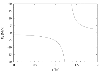
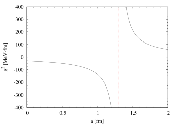
As an explicit demonstration of this behavior we consider the case of $S$-wave $np$ scattering. In this case the low-energy parameters are $a_{0}=-23.7$ fm and $r_{0}=2.75$ fm Hackenburg:2006qd . The expressions in Eqs. (12) and (13) are shown in Figs. 3 and 3, respectively, for this case.

We see from the figures that both $E_{\lambda}(a)$ and $g^{2}(a)$ are positive above the pole at $a_{p}=1.30$ fm, and both are negative below the pole. At $a=0$, they have the values $E_{\lambda}(0)=-1.27$ MeV and $g^{2}(0)=-30.2$ MeV-fm [$g^{2}(0)/(\hbar c)=-0.153$]. Since $g^{2}$ is negative for $a<a_{p}$, so is $\gamma^{2}=g^{2}/a$. Hence, the conventional $R$-matrix description with $\gamma^{2}>0$ is not possible with a channel radius less than $a_{p}=1.30$ fm.

A similar situation obtains for the ${}^{3}\!S_{1}$ case, where the scattering length and effective range are 5.411 fm and 1.74 fm Hackenburg:2006qd , respectively. In this case, the pole is located at 1.07 fm. In distinction to the ${}^{1}\!S_{0}$ case, the scattering length and effective range are both positive. This implies that the $R$-matrix parameters, $E_{\lambda}(0)$ and $g^{2}(0)$, now take the values $+8.81$ MeV and $-47.7$ MeV-fm [$g^{2}(0)/(\hbar c)=-0.242$], respectively.

III Two-channel description of the $dt$ reaction

The single-level, two-channel formula LT58 for the $J^{\pi}=3/2^{+}$ ³H$(d,n)^{4}$He reaction cross section is

$$\sigma^{3/2^{+}}_{n,d}= \frac{4\pi}{k_{d}^{2}}\frac{2}{3}P_{n}P_{d}\gamma_{n}^{2}\gamma_{d}^{2}\left|E_{\lambda}-E-\gamma_{d}^{2}(S_{d}-B_{d})\right.$$

$$\left.-\gamma_{n}^{2}(S_{n}-B_{n})-i(\gamma_{d}^{2}P_{d}+\gamma_{n}^{2}P_{n})\right|^{-2},$$ (15)

with $S_{c}$ and $P_{c}$ ($c=n,d$) the real and imaginary parts, respectively, of the dimensionless outgoing-wave logarithmic derivative,

$$L_{c}=\frac{a_{c}}{O_{c}}\frac{\partial O_{c}}{\partial r_{c}}\Bigg{|}_{r_{c}=a_{c}}.$$ (16)

The boundary condition numbers $B_{d}$ and $B_{n}$ are real constants that are, in principle, arbitrary and can be chosen for convenience, as discussed below. We will make these choices in order to match the field-theoretical expression as the radii approach zero, as described in Section III.2. For the charged $dt$ channel, the penetrability, $P_{d}$ and the shift function, $S_{d}$ are given in terms of Coulomb functions by

$$P_{d} =\frac{\rho_{d}}{F_{0}^{2}+G_{0}^{2}},$$ (17)

$$S_{d} =(F_{0}F_{0}^{\prime}+G_{0}G_{0}^{\prime})P_{d},$$ (18)

where $F_{0}=F_{0}(\rho_{d},\eta_{d})$ and $G_{0}=G_{0}(\rho_{d},\eta_{d})$ are, respectively, the regular and irregular Coulomb functions for $\ell=0$, with $\rho_{d}=k_{d}a_{d}$ and $\eta_{d}=e^{2}\mu_{d}/(\hbar^{2}k_{d})$. Here, $k_{d}$ is the center-of-mass wave number in the $dt$ channel (previously called $p_{dt}$ BH13 ), $\mu_{d}=m_{d}m_{t}/(m_{d}+m_{t})$ its reduced mass (previously called $m_{dt}$), and $a_{d}$ is its channel radius. The prime means the derivative with respect to $\rho_{d}$. Similar quantities are defined for the $n\alpha$ channel in terms of the Riccati-Bessel functions for orbital angular momentum, $\ell=2$, are given as

$$P_{n} =\frac{\rho_{n}}{u_{2}^{2}+v_{2}^{2}},$$ (19)

$$S_{n} =(u_{2}u_{2}^{\prime}+v_{2}v_{2}^{\prime})P_{n},$$ (20)

with $u_{2}=\rho_{n}j_{2}(\rho_{n})$ and $v_{2}=-\rho_{n}n_{2}(\rho_{n})$, $j_{2}$ and $n_{2}$ being the ordinary regular and irregular spherical Bessel functions. Here the prime means derivative with respect to $\rho_{n}=k_{n}a_{n}$, with $k_{n}$ the center-of-mass wave number (previously $p_{n\alpha}$) and channel radius $a_{n}$ in the $n\alpha$ channel.

Aside from the channel radii $a_{c}$, the remaining $R$-matrix parameters in the single-level expression (III) are the reduced-width amplitudes $\gamma_{c}$ for $c=d,n$, and the energy eigenvalue $E_{\lambda}$. All of these are real parameters as a result of the assumed Hermiticity of the interaction Hamiltonian and the chosen conditions on the wave functions at the boundary of the interior region.

III.1 Finite channel radii

The original formulation of $R$-matrix theory of Wigner and Eisenbud WE47 is based upon the separation into interior (strongly interacting) and exterior (non-strong) regions of the configuration space of nucleons for each channel partition (pair). $R$-matrix theory is, by this formulation, a finite-range ($a_{c}>0$) description of nuclear reactions. However, as we will see in the following section, one may sensibly take the zero-radius limit of the theory. In so doing, we reproduce the EFT expressions for the cross section [see Eq.(III.2)] that follow from a quantum effective field theory of particles interacting via local interactions. As shown in the companion paper BH13 , a high-quality fit to the ³H$(d,n)^{4}$He reaction data within the EFT treatment required the sign of the energy shift, $\Re[\Sigma_{dt}^{(C)}(W)]$, to be changed. This led to the use of the “wrong-sign” Lagrangian in the EFT approach, as described there. The wrong-sign Lagrangian can be alternatively and equivalently interpreted as having pure-imaginary coupling constants. Based on the identity of the EFT and $R$-matrix expressions for the ³H$(d,n)^{4}$He reaction cross section (see below), we anticipated that, as the $R$-matrix radii are taken to zero, the reduced-width amplitudes $\gamma_{c}$ would become pure imaginary numbers. It is instructive to study the nature of the transition from real to pure-imaginary values of the $\gamma_{c}$ in $R$-matrix theory, where the full two-channel $R$ matrix is used, in order to better understand its relation to an “unphysical” Lagrangian in EFT.

We therefore conducted a numerical study of the dependence on channel radii of the two-channel $R$-matrix fit to the $dt$ reaction cross section. The cross section data fitted with Eq.(III) were the same ones Arn54 ; Jar84 ; Brn87 used for the EFT fit, employing a Mathematica program that could easily be extended to complex values of some of the parameters. It was found that no meaningful reduction in the $\chi^{2}$ was achieved by allowing separate values of the channel radii, so the fits were made with $a_{d}=a_{n}=a$. The boundary condition numbers $B_{c}$ were taken to be the energy-independent part of the shift function, as given by Eq.(40) in the Appendix. This gives $B_{n}=-2$ independent of $a$, but $B_{d}=-x_{0}K_{0}(x_{0})/(2K_{1}(x_{0}))$, $K_{n}$ being the irregular modified Bessel function evaluated at $x_{0}=\sqrt{8a/b_{0}}$, which depends on $a$. Here, $b_{0}=34.62$ fm is a length for the $dt$ system equivalent to the Bohr radius.

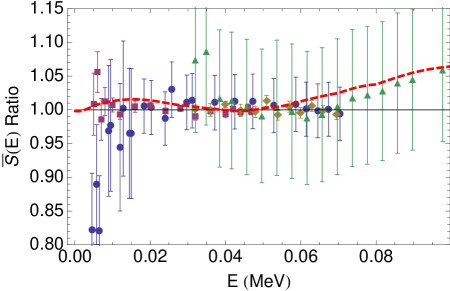
The best fit ($\chi^{2}=34.94$ corresponding to a $\chi^{2}/$DOF = 0.713) was obtained for $a=7$ fm, although $\chi^{2}$ was a shallow function of $a$ in the range $a=3$ to 8 fm. The best-fit parameters for $a=7$ fm and boundary conditions $B_{d}=-0.59,B_{n}=-2$ are: $E_{\lambda}=179\pm 5$ keV, $\gamma_{d}^{2}=324\pm 12$ keV, $\gamma_{n}^{2}=12.2\pm 0.2$ keV. This best single-level fit to the experimental $dt$ data is shown in Fig. 4, which displays the data divided by the theoretical fit. Thus the theory appears simply as the horizontal line at the ordinate 1.00. (All the quantities were first expressed in terms of the dimensionless astrophysical $S$ factor $\overline{S}$ defined in Eq.(1.11) of Ref.BH13 .) Also shown are the results of Bosch and Hale (BH) B&H92 divided by the single-level fit. They are close to the single-level fit at low energies, but their ratio to it increases at higher energies.

Figure 4: The $d+t$ reaction data divided by the single-level, four-parameter $R$-matrix fit described in the text. The (blue) circles are the data of Arnold et al. Arn54 ; the (magenta) squares are the data of Jarmie et al. Jar84 renormalized by a factor of 1.017; the (olive) diamonds are the relative data of Brown et al. Brn87 renormalized by a factor of 1.025; the (green) triangles are the data of Argo et al. Arg52 , which were not included in the single-level fit because of their large error bars. This fit yields a $\chi^{2}$ per degree of freedom of 0.713 which is to be compared with the value of 0.784 determined in the three-parameter EFT fit of Ref.BH13 . The red dashed curve presents the results of the $R$-matrix fit of Bosch and Hale B&H92 divided by the single-level four parameter fit.

For solutions near $a=2$ fm, the three fitting parameters became quite large in magnitude, while maintaining the same signs they had at larger radii. However, for $a<2$ fm, roughly comparable fits were obtained to the data with the signs of all the parameters changed ($E_{\lambda}<0,\gamma_{c}^{2}<0$). This behavior is consistent with having gone through a pole at $a_{p}$ somewhat less than 2 fm, and having pure-imaginary reduced-width amplitudes $\gamma_{c}$ at zero radius, in qualitative agreement with the wrong-sign Lagrangian EFT result, and similar to the case of $np$ scattering discussed in Sec.II. In the next section, we will show that this agreement between the $R$-matrix description at zero radius and the EFT result is exact.

III.2 Taking the zero-radius limit

In order to match to the EFT expression, including a single unstable, intermediate field, for the cross section Eq. (4.5) from Ref.BH13 , we make the associations

$$\gamma_{d}^{2}=-\frac{g_{d}^{2}}{2\pi}\frac{\mu_{d}}{\hbar^{2}a_{d}}~{}{\rm and}~{}\gamma_{n}^{2}=-\frac{g_{n}^{2}}{6\pi}\frac{\mu_{n}}{\hbar^{2}a_{n}^{5}}$$ (21)

between the reduced widths $\gamma_{c}^{2}$ and squared EFT coupling constants $g_{c}^{2}$, and let the channel radii $a_{c}$ approach zero. The minus signs are necessary to account for the wrong-sign Lagrangian convention used in Ref.BH13 , in which the coupling constants $g_{c}$ are assumed to be real, rather than pure imaginary. Although in this small-$a_{c}$ limit the $R$-matrix reduced-width amplitudes $\gamma_{c}$ become infinite as the penetrabilities $P_{c}$ approach zero, we expect the “half-width” terms in both the numerator and denominator of the cross section expression

$$\gamma_{d}^{2}P_{d} \rightarrow-\frac{g_{d}^{2}}{2\pi}\frac{\mu_{d}}{\hbar^{2}}k_{d}C_{0}^{2}(\eta_{d}),$$ (22)

$$\gamma_{n}^{2}P_{n} \rightarrow-\frac{g_{n}^{2}}{6\pi}\frac{\mu_{n}}{\hbar^{2}}k_{n}^{5},$$ (23)

to remain finite. Here, $C_{0}^{2}(\eta)=2\pi\eta[\exp(2\pi\eta)-1]^{-1}$ is called $|\psi_{{\bf p}_{dt}}^{(C)}(0)|^{2}$ in the companion paper. Additionally, we choose the channel-surface boundary conditions, $B_{n,d}$, to be the energy-independent part of the shift functions at zero energy, $S_{c}^{\infty}=S_{\ell(c)}(\infty,a)$, as is written in the Appendix. That is, we choose $B_{n}=S_{n}^{\infty}$ and $B_{d}=S_{d}^{\infty}$, so that the energy shift of $E_{\lambda}$ in the denominator of Eq. (III),

$$\Delta =-\gamma_{d}^{2}(S_{d}-B_{d})-\gamma_{n}^{2}(S_{n}-B_{n}),$$ (24)

depends on quantities $\tilde{S_{c}}=S_{c}-S_{c}^{\infty}$ that satisfy a dispersion relation (see the Appendix). $\tilde{S_{n}}$ vanishes in the $n\alpha$ channel, leaving only the energy-dependent shift in the $dt$ channel, given according to Eqs. (A) of the Appendix and Section III.1 above by

$$\Delta_{d}(E)=-\gamma_{d}^{2}\tilde{S_{d}}\rightarrow\frac{g_{d}^{2}}{\pi}\frac{\mu_{d}}{\hbar^{2}b_{0}}[\Re\psi(i\eta_{d})-\ln(\eta_{d})].$$ (25)

We note that the associations above allow us to connect with the Coulomb self-energy of the previous paperBH13 ,

$$\gamma_{d}^{2}\bar{L}_{d}\rightarrow-\frac{g_{d}^{2}}{2\pi}\frac{\mu_{d}}{\hbar^{2}a_{d}}(\bar{S}_{d}+iP_{d})=\Sigma_{dt}^{(C)}.$$ (26)

Using these limiting values, the $R$-matrix cross section expression, Eq.(III) becomes

$$\sigma^{3/2^{+}}_{n,d} =\frac{32\pi}{9\hbar v_{d}}\frac{g_{d}^{2}}{4\pi}\frac{g_{n}^{2}}{4\pi}\frac{\mu_{n}}{\hbar^{2}}k_{n}^{5}C_{0}^{2}(\eta_{d})$$

$$\times\Bigg{|}E-E_{\lambda}-\Delta_{d}(E)$$

$$-i\left[\frac{g_{d}^{2}}{2\pi}\frac{\mu_{d}}{\hbar^{2}}k_{d}C_{0}^{2}(\eta_{d})+\frac{g_{n}^{2}}{6\pi}\frac{\mu_{n}}{\hbar^{2}}k_{n}^{5}\right]\Bigg{|}^{-2},$$ (27)

which is in complete agreement with Eqs. (1.6)–(1.9) in Ref.BH13 , keeping in mind that $E=\frac{{\bf p}_{dt}^{2}}{2m_{dt}}$, $E_{\lambda}=E_{*}$, and $\Delta_{d}(E)=\frac{g_{dt}^{2}}{4\pi}\Delta(W)$.

IV discussion and conclusions

This investigation has revealed some interesting, and possibly significant, connections of single-level $R$-matrix theory to other theoretical approaches. It is apparent that the experimental data for the two cases considered, $np$ scattering and the $dt$ reaction, dictate minimum channel radii at which the $R$-matrix parameters are physical. For $np$ scattering, this radius is just above 1 fm, and for the $dt$ reaction, it is just below 2 fm. This finding is consistent with the presumptive connection of the channel radii with the range of nuclear forces. What is surprising, however, is that one can continue the $R$-matrix parameters below the pole that occurs at these minimum radii [c.f. Figs. 3 and 3], and obtain equally good fits to the experimental data with negative reduced widths $\gamma^{2}$. The continuation to zero radius done in this way gives identically the same result as does effective field theory with a wrong-sign Lagrangian, in which local interactions are mediated by a single unstable field.

While it appears that the position of the poles is related to the range of nuclear forces, we currently lack a complete understanding of the physical significance of the pole in the dependence of the single-level $R$-matrix parameters on channel radius. However, the presence of this singularity separating the physical and non-physical descriptions of the experimental data using $R$-matrix theory gives an indication of how to interpret the wrong-sign Lagrangian in effective field theory: imaginary coupling constants in the field theory, which are equivalent to the wrong-sign free-field Lagrangian, appear to compensate for a description of the finite-range (nuclear) forces with zero-range interactions. A direct correspondence of the reduced-width amplitudes in $R$-matrix theory to the coupling constants of EFT as discussed in Section III of this paper appears in the limit of vanishing channel radii.

For the $dt$ reaction, the extrapolation to zero radius gives a description that is similar to the “model-independent” effective range expansion of Karnakov et al. Karnakov90 . However, the description given here and in the companion paper BH13 requires only three parameters, whereas that of Ref.Karnakov90 employs four parameters, which is the number required for a single-level $R$-matrix description at finite radii.

The present study establishes an identity between the EFT treatment of light nuclear reactions with an unstable intermediate field using local interactions with that of the single-level, two-channel $R$ matrix in the limit in which the channel radii are taken to zero. We have found that poles in the level energy and channel widths appear in the continuation in channel radii between this limit and radii that correspond to real, physical values of the widths. The question of the physical interpretation of such poles is beyond the scope of this work. Among the questions raised by the poles is the issue of whether the poles arise due to the restriction to a single-level $R$-matrix description. We are currently studying this question using potential models.

Appendix A Dispersion relations for the outgoing-wave logarithmic derivative

A quantity of central importance in this discussion is the outgoing-wave logarithmic derivative of Eq. (16),

$$L_{c}=\frac{a_{c}}{O_{c}}\frac{\partial O_{c}}{\partial r_{c}}\Bigg{|}_{r_{c}=a_{c}}=S_{c}+iP_{c}.$$ (28)

For charged-particle channels such as $dt$, the outgoing-wave solution is defined in terms of Coulomb functions by

$$O_{d}=(G_{0}+iF_{0})\exp(-i\sigma_{0}),$$ (29)

with $\sigma_{0}=\arg\Gamma(1+i\eta_{d})$ the $S$-wave Coulomb phase shift. For the neutral-particle $n\alpha$ channel, it is defined in terms of the Riccati-Bessel functions for $\ell=2$,

$$O_{n}=-i\rho_{n}[j_{2}(\rho_{n})+in_{2}(\rho_{n})]=-i\rho_{n}h^{+}_{2}(\rho_{n}),$$ (30)

where $j_{2}$ and $n_{2}$ are the ordinary regular and irregular spherical Bessel functions, respectively, $h^{+}_{2}$ is the outgoing Hankel function of second order, and $\rho_{n}=k_{n}a_{n}$, the product of the wave number in the center-of-mass, $k_{n}$ and channel radius $a_{n}$ in the $n\alpha$ channel.

It is useful for this application to develop a dispersion relation for the real and imaginary parts of $L_{c}$. Ordinarily, this would be done by means of a Hilbert transform that depends on the analytic properties of $L_{c}(E)$ in the cut $E$-plane. The fact that the the outgoing-wave logarithmic derivative diverges as $|E|\rightarrow\infty$ [see Eq.(31) below], however, prevents a direct application of the Hilbert transform in the complex-$E$ plane. Since this function is finite for all values of $\ell$ for $E=0$, it makes sense to consider a Hilbert transform for it in the inverse energy. This procedure is slightly different for Hankel functions (neutral-particle channels) and Coulomb functions (charged-particle channels), so they will be addressed separately.

We first consider the neutral case and explicitly display only the dependence of the channel $c$ [as in Eq.(28)] on the orbital angular momentum $\ell$. The $n\alpha$ $\tfrac{3}{2}^{+}$ channel, for example, has $\ell=2$, and we examine $L_{2}(\rho_{n})=\rho_{n}h_{2}^{+^{\prime}}(\rho_{n})/h_{2}^{+}(\rho_{n})$, where the prime means differentiation with respect to $\rho_{n}$. It can be written as

$$L_{2}(\rho_{n})=-2+\frac{1-i\rho_{n}}{\frac{3}{\rho_{n}^{2}}-\frac{3i}{\rho_{n}}-1},$$ (31)

which shows that $\tilde{L}_{2}(\rho_{n})=L_{2}(\rho_{n})+2$ is finite (zero, in fact) at infinity in $x=\rho_{n}^{-2}$. A less obvious consequence of using inverse energy variables is that, whereas the integration contour for the Hilbert transform would be taken on the first sheet in energy variables, it must be taken on the second sheet in the inverse-energy variable $\rho_{n}^{-2}$. Furthermore, since on that sheet the positive $\rho_{n}^{-1}$ axis lies on the bottom rim of the cut, we must approach the cut from below to get the physical values. Therefore, the Hilbert transform for $\tilde{L}_{2}(\rho_{n})$ has the form in the cut $x$-plane of

$$\tilde{L}_{2}(\rho_{n})=-\frac{1}{\pi}\int_{0}^{\infty}dx\frac{\Im\tilde{L}_{2}(x)}{x-\rho_{n}^{-2}+i\epsilon}.$$ (32)

Using the familiar Plemelj relation

$$\frac{1}{x-x_{0}+i\epsilon}=\frac{P}{x-x_{0}}-i\pi\delta(x-x_{0})\,,$$ (33)

the above expression reduces to an identity for the imaginary part of $\tilde{L}_{2}$, but for the real part yields the relation:

$$\Re\tilde{L}_{2}(\rho_{n}) =S_{2}(\rho_{n})+2$$

$$=-\frac{1}{\pi}\mathchoice{{\vbox{\hbox{$\textstyle-$}}\kern-4.86108pt}}{{\vbox{\hbox{$\scriptstyle-$}}\kern-3.25pt}}{{\vbox{\hbox{$\scriptscriptstyle-$}}\kern-2.29166pt}}{{\vbox{\hbox{$\scriptscriptstyle-$}}\kern-1.875pt}}\!\int dx\frac{P_{2}(x)}{x-\rho_{n}^{-2}},$$ (34)

where $\mathchoice{{\vbox{\hbox{$\textstyle-$}}\kern-4.86108pt}}{{\vbox{\hbox{$\scriptstyle-$}}\kern-3.25pt}}{{\vbox{\hbox{$\scriptscriptstyle-$}}\kern-2.29166pt}}{{\vbox{\hbox{$\scriptscriptstyle-$}}\kern-1.875pt}}\!\int$ is the Cauchy principal value. This result can be generalized for uncharged channels to the desired dispersion relation between the real and imaginary parts of $L_{\ell}$,

$$S_{\ell}(\rho)=-\ell-\frac{1}{\pi}\mathchoice{{\vbox{\hbox{$\textstyle-$}}\kern-4.86108pt}}{{\vbox{\hbox{$\scriptstyle-$}}\kern-3.25pt}}{{\vbox{\hbox{$\scriptscriptstyle-$}}\kern-2.29166pt}}{{\vbox{\hbox{$\scriptscriptstyle-$}}\kern-1.875pt}}\!\int dx\frac{P_{\ell}(x)}{x-\rho^{-2}}.$$ (35)

As a check for $\ell=2$, we write Eq. (31) in terms of $x$ and resolve it into real and imaginary parts:

$$\tilde{L}_{2}(x)=\frac{3x+2+ix^{-1/2}}{9x^{2}+3x+1}.$$ (36)

Then Eq. (32) implies the relation between the real and imaginary parts

$$\frac{3y+2}{9y^{2}+3y+1}$$

$$=-\frac{1}{\pi}\mathchoice{{\vbox{\hbox{$\textstyle-$}}\kern-4.86108pt}}{{\vbox{\hbox{$\scriptstyle-$}}\kern-3.25pt}}{{\vbox{\hbox{$\scriptscriptstyle-$}}\kern-2.29166pt}}{{\vbox{\hbox{$\scriptscriptstyle-$}}\kern-1.875pt}}\!\int dx\frac{x^{-1/2}}{(x-y)(9x^{2}+3x+1)},$$ (37)

which is easily verified by performing the principal-value integral.

For Coulomb functions, the natural inverse-energy variable to use for the Hilbert transform is $\eta^{2}=\frac{e^{2}}{2b_{0}E}$, with $b_{0}=\frac{\hbar^{2}}{e^{2}\mu}$ the equivalent of the Bohr radius for the initial pair of charged particles. Then the conventional variable $\rho=ka$ is determined by $k=(\eta b_{0})^{-1}$. Therefore, we expect the Hilbert transform and a dispersion relation analogous to Eqs. (32) and (35) for Coulomb functions at a finite radius $r=a$ to be

$$L_{\ell}(\eta,a) =S_{\ell}(\infty,a)$$

$$-\frac{1}{\pi}\int_{0}^{\infty}dx\frac{P_{\ell}(x,a)}{x-\eta^{2}+i\epsilon},$$ (38)

$$S_{\ell}(\eta,a) =S_{\ell}(\infty,a)-\frac{1}{\pi}\mathchoice{{\vbox{\hbox{$\textstyle-$}}\kern-4.86108pt}}{{\vbox{\hbox{$\scriptstyle-$}}\kern-3.25pt}}{{\vbox{\hbox{$\scriptscriptstyle-$}}\kern-2.29166pt}}{{\vbox{\hbox{$\scriptscriptstyle-$}}\kern-1.875pt}}\!\int dx\frac{P_{\ell}(x,a)}{x-\eta^{2}},$$ (39)

where $S_{\ell}(\infty,a)$ is a real constant that gives the value of $L_{\ell}$ at infinite $\eta$ (zero energy). For Hankel functions, this is simply $S_{\ell}(\infty)=-\ell$, but for Coulomb functions it is given by

$$S_{\ell}(\infty,a)=-\ell-\frac{x_{0}}{2}\frac{K_{2\ell}(x_{0})}{K_{2\ell+1}(x_{0})},$$ (40)

with $K_{n}(x_{0})$ the irregular modified Bessel function evaluated at $x_{0}=\sqrt{8a/b_{0}}$.

The validity of these relations is difficult to test in general, but one of the results in our companion paper [Eq.(4.19)] is a special case of this Coulomb function dispersion relation. In that case, we want to find the shift function that belongs with the $dt$ penetrability function at vanishingly small radius $a_{d}$,

$$P_{d}(\eta)\approx\rho_{d}C_{0}^{2}(\eta)=\frac{2\pi a_{d}/b_{0}}{\exp(2\pi\eta)-1}.$$ (41)

This sort of penetrability function occurs in the integral representation of the digamma function,

$$\psi(z) =\ln(z)-\frac{1}{2z}$$

$$-\int_{0}^{\infty}dt^{2}\frac{1}{t^{2}+z^{2}}\frac{1}{\exp(2\pi t)-1}.$$ (42)

Letting $z=i\eta+\epsilon/(2\eta)$, with $\epsilon$ a positive infinitesimal ($\Re z>0$ is required for the validity of the above expression), we have

$$\psi(i\eta) =\ln(i\eta)-\frac{1}{2i\eta}$$

$$-\int_{0}^{\infty}dt^{2}\frac{1}{t^{2}-\eta^{2}+i\epsilon}\frac{1}{\exp(2\pi t)-1},$$ (43)

which has the form of Eq. (A) for the penetrability in Eq. (41), with $x=t^{2}$ and $l=0$.

The shifted logarithmic derivative,

$$\tilde{L}_{d}=S_{d}-S_{d}^{\infty}+iP_{d},$$ (44)

with

$$S_{d}^{\infty} =S_{0}(\eta\rightarrow\infty,a_{d}\rightarrow 0)$$

$$=(2a_{d}/b_{0})[\ln(2a_{d}/b_{0})+2\gamma]\rightarrow 0,$$ (45)

can therefore be expressed as the Hilbert transform based on rearranging Eq. (A),

$$\frac{b_{0}}{2a_{d}}\tilde{L}_{d}(\eta) =-\int_{0}^{\infty}dt^{2}\frac{1}{t^{2}-\eta^{2}+i\epsilon}\frac{1}{\exp(2\pi t)-1}$$

$$=\psi(i\eta)-\ln(i\eta)+\frac{1}{2i\eta}.$$ (46)

Using properties of the digamma function AS , we have

$$\frac{b_{0}}{2a_{d}}\Im\tilde{L}_{d}(\eta)=\Im\psi(i\eta)-\frac{\pi}{2}-\frac{1}{2\eta},$$ (47)

and since

$$\Im\psi(i\eta)=\frac{1}{2\eta}+\frac{\pi}{2}\frac{\exp(2\pi\eta)+1}{\exp(2\pi\eta)-1},$$ (48)

it gives the check that

$$\frac{b_{0}}{2a_{d}}\Im\tilde{L}_{d}(\eta) =\frac{\pi}{2}\left(\frac{\exp(2\pi\eta)+1}{\exp(2\pi\eta)-1}-1\right)$$

$$=\frac{\pi}{\exp(2\pi\eta)-1}=\frac{b_{0}}{2a_{d}}P_{d}.$$ (49)

The new relation we want, however, is given by

$$\frac{b_{0}}{2a_{d}}\Re\tilde{L}_{d}(\eta) =\frac{b_{0}}{2a_{d}}\tilde{S_{d}}$$

$$=\Re\psi(i\eta)-\ln(\eta)=h(\eta),$$ (50)

which agrees with the energy-dependent part of direct expansions (e.g., Jackson and Blatt JB ) of the $\ell=0$ Coulomb wave functions for small $a_{d}$, and with Eq. (4.19) of Ref.BH13 .

References

- (1) L.S. Brown and G.M. Hale, Phys. Rev. C (preceeding paper).
- (2) R.M. White, D.A. Resler and S.I. Warshaw, Nucl. Data Sci. Tech., pp.834–839, (Springer, 1992).
- (3) B.M. Karnakov, V.D. Mur, S.G. Pozdnyakov, and V.S. Popov, JETP Lett., 51, 399 (1990) [Pis’ma Zh. Eksp. Teor. Fiz. 51, 352 (1990)].
- (4) B.M. Karnakov, V.D. Mur, S.G. Pozdnyakov, and V.S. Popov, JETP Lett., 54, 127 (1991) [Pis’ma Zh. Eksp. Teor. Fiz. 54, 131 (1991)].
- (5) E.P. Wigner and L. Eisenbud, Phys. Rev. 72, 29 (1947).
- (6) See, for example, E. Epelbaum, H. Hammer, and U.-G. Meissner, Rev. Mod. Phys. 81, 1773 (2009).
- (7) R.W. Hackenburg, Phys. Rev. C 73, 044002 (2006).
- (8) A.M. Lane and R.G. Thomas, Rev. Mod. Phys. 30, 322 (1958), Eq. (XII,1.13), p. 322.
- (9) H.-S. Bosch and G.M. Hale, Nucl. Fusion 32, 611 (1992); The multilevel, multichannel -matrix analysis of the 5He system, on which the Bosch and Hale cross sections are based, includes data for and elastic scattering, in addition to those for the reaction, at energies equivalent to up to 11 MeV. It fits the 2665 data points included using 117 free parameters with a per degree of freedom of 1.56.
- (10) W.R. Arnold, J.A. Phillips, G.A. Saywer, E.J. Stovall, Jr., and J.L. Tuck, Phys. Rev. 93, 483 (1954).
- (11) N. Jarmie, R.E. Brown, and R.A. Hardekopf, Phys. Rev.C 29, 2031 (1984); These data were renormalized by a factor of 1.017.
- (12) R.E. Brown, N. Jarmie, and G.M. Hale, Phys. Rev. C 35, 1999 (1987); These relative data were renormalized by a factor of 1.025.
- (13) H.V. Argo, R.F. Taschek, H.M. Agnew, A. Hemmendinger and W.T. Leland, Phys. Rev. 87, 612 (1952).
- (14) M. Abramowitz and I.A. Stegun, Eds, Handbook of Mathematical Functions, p.259 (Dover Pub., New York, 1972).
- (15) J.D. Jackson and J.M. Blatt, Rev. Mod. Phys. 22, 77 (1950).