Suzaku Observations of the X-ray Brightest Fossil Group ESO 3060170

Abstract

“Fossil” galaxy groups, each dominated by a relatively isolated giant elliptical galaxy, have many properties intermediate between groups and clusters of galaxies. We used the Suzaku X-ray observatory to observe the X-ray brightest fossil group, ESO 3060170, out to $R_{200}$, in order to better elucidate the relation between fossil groups, normal groups, and clusters. We determined the intragroup gas temperature, density, and metal abundance distributions and derived the entropy, pressure and mass profiles for this group. The entropy and pressure profiles in the outer regions are flatter than in simulated clusters, similar to what is seen in observations of massive clusters. This may indicate that the gas is clumpy and/or the gas has been redistributed. Assuming hydrostatic equilibrium, the total mass is estimated to be $\sim 1.7\times 10^{14}$ $M_{\odot}$ within a radius $R_{200}$ of $\sim 1.15$ Mpc, with an enclosed baryon mass fraction of 0.14. The integrated iron mass-to-light ratio of this fossil group is larger than in most groups and comparable to those of clusters, indicating that this fossil group has retained the bulk of its metals. A galaxy luminosity density map on a scale of 25 Mpc shows that this fossil group resides in a relatively isolated environment, unlike the filamentary structures in which typical groups and clusters are embedded.

1 Introduction

In the hierarchical structure formation scenario, galaxy systems evolve through mergers and accretion, with galaxy groups regarded as the building blocks of galaxy clusters. However, X-ray observations of groups and clusters suggest that clusters are not simply scaled-up versions of present-day groups. To date, most X-ray observations of the gas in groups and clusters of galaxies have been restricted to within $\sim R_{500}$, the radius (typically $0.4-1.3$ Mpc) within which the average density is 500 times the cosmological critical density. Based on X-ray observations within $\sim R_{500}$, clusters appear to differ from groups in several ways. 1) The baryonic mass fraction in clusters varies only weakly with cluster temperature, with values nearly equal to the cosmological value of $f_{b}=0.15$ (Planck Collaboration 2013); however, the baryon fraction in groups ranges widely ($f_{b}\sim 0.04-0.1$), with values typically much smaller than the cosmological value and rising with group temperature (Dai et al. 2010). 2) Clusters have about the same ratio of gaseous iron mass to stellar light, regardless of their temperature, while in groups the iron-mass-to-light ratio (IMLR) drops precipitously with gas temperature when $kT\lesssim 1$ keV; galaxy groups have up to 50 times less iron per unit optical luminosity than clusters (Renzini 1997). 3) Scaling relations involving X-ray luminosity, gas temperature, entropy, and mass differ between clusters and groups (Voit et al. 2005). Based on the studies cited above, we adopt $\sim$ 2 keV for the boundary between galaxy groups and clusters.

All of these differences between groups and clusters may have the same origin: the gravitational potential wells of clusters are deep enough that they have retained the bulk of their baryons, including gas enriched by supernovae ejecta; however, the shallower potential wells of groups make them more vulnerable to gas loss due to energy input from nongravitational processes such as galactic winds and feedback from active galactic nuclei (AGN) (Sun 2012). This account needs to be confirmed with deep observations of the outer parts of galaxy groups to test whether the “missing” baryons and metals can be found in the outer atmospheres of groups.

Thanks to a low and stable instrumental background, the Suzaku X-ray satellite observatory has been able to observe a number of massive clusters out to their virial radii or even beyond (Bautz et al. 2009; George et al. 2009; Hoshino et al. 2010; Kawaharada et al. 2010; Simionescu et al. 2011; Reiprich et al. 2009; Sato et al. 2012; Walker et al. 2012a,b). Baryon mass fractions are observed to reach the cosmological value or even greater (Simionescu et al. 2011; Sato et al. 2012). Metals are reported to be found at the virial radii of several clusters (Fujita et al. 2008; George et al. 2009; Simionescu et al. 2011; Urban et al. 2011). Surprisingly, gaseous entropy profiles are found to flatten beyond $\sim$ $R_{500}$, contrary to expectations from numerical simulations which show entropy rising nearly linearly with radius: $S\sim r^{1.1}$ (Voit et al. 2005). The observed entropy flattening has been interpreted in various ways: 1) it may be due to clumped gas, which would increase the emission-measure-weighted gas density over the actual average gas density (Simionescu et al. 2011); 2) the entropy flattening may arise from electrons being out of thermal equilibrium with ions, due to recent accretion shocks in cluster outskirts (Hoshino et al. 2010; Akamatsu et al. 2011); 3) the weakening of accretion shocks in relaxed clusters may reduce the entropy at large radii (Cavaliere et al. 2011, Walker et al. 2012c). Despite there being many more groups than clusters, there are currently not many X-ray observations of groups or poor clusters out to their virial radii, due to their relatively low surface brightness.

A particularly interesting subset of such galaxy systems are fossil groups, which are empirically defined as systems with 1) a central dominant galaxy more than two optical magnitudes brighter than the second brightest galaxy within half a virial radius; and 2) an extended thermal X-ray halo with $L_{\rm(X,bol)}$ $>$ $10^{42}$ $h_{50}^{-2}$ erg s^-1 (Jones et al. 2003). A fossil group is thought to be the evolutionary end-result of a group of galaxies having mostly merged into one giant elliptical (Mulchaey & Zabludoff 1999). Fossil groups are not rare — they are estimated to constitute 8-20% of groups and clusters (Jones et al. 2003). Yang et al. (2008) used the Sloan Digital Sky Survey (SDSS) to show that 20%–60% of groups with masses $\approx 10^{13}M_{\odot}$ are fossil groups. Simulations predict that about 33% of groups are fossil groups (D’Onghia et al. 2005). The properties of fossil groups generally populate the transition regions in the scaling relations for groups and clusters (Khosroshahi et al. 2007; Proctor et al. 2011; Miller et al. 2012). More than half have $kT\gtrsim 2$ keV, which is high for groups and more typical of poor clusters (Khosroshahi et al. 2007; Vikhlinin et al. 1999).

There are multiple lines of evidence suggesting that fossil groups tend to be old, relaxed systems. For example, X-ray observations show that fossil groups are associated with unusually concentrated dark matter distributions (Khosroshahi et al. 2007; von Benda-Beckmann et al. 2008), which are associated with earlier formation epochs in numerical simulations (Giocoli et al. 2012; Dariush et al. 2007). Secondly, the optical isophotes and X-ray atmospheres of fossil groups tend to appear undisturbed, implying that their last significant mergers were long ago. Moreover, simulations by D’Onghia et al. (2005) showed that groups with earlier formation times have larger luminosity differences between their 1st and 2nd brightest galaxies. However, some observational evidence suggests that fossil groups may have formed or been significantly disturbed more recently. For example, fossil groups tend not to have very extensive cool cores, despite their central cooling times being less than the Hubble time (Miller et al. 2012). In addition, Dupke et al. (2010) showed that there is an enhancement of SNII ejecta in the central regions of some fossil groups, perhaps due to star formation triggered by recent mergers forming their central dominant galaxies. Interestingly, von Benda-Beckmann et al. (2008) showed in simulations tracking fossil groups forward in time that the majority had their luminosity gap (between 1st and 2nd-brightest galaxies) filled by new infalling galaxies; this suggests that fossil groups are a transitional phase, not the stable end-result of a merging group.

To understand the evolution and nature of fossil groups, it is crucial to understand how their structure and environment compare to those of non-fossil systems. A key strategy is to explore the outer regions of the group gas, using similar methods to those described above. This has been previously done for fossil group RXJ 1159+5531 by Humphrey et al. (2012), who trace the group gas out to $R_{\rm vir}=R_{108}$. They find no flattening of the entropy profile and no need to invoke gas clumping, indicating that this phenomenon might depend on the environment or evolutionary state of the system. The baryon fraction of RXJ 1159+5531 is consistent with the cosmological value, much larger than what has been observed in normal groups at smaller radii. Studies of additional systems are clearly needed to further constrain the fossil group paradigm.

To learn more about the nature of fossil groups, we performed a deep study of the X-ray brightest fossil group, ESO 3060170, with Suzaku. ESO 3060170 was first selected as a fossil group candidate from a sample of early-type galaxies observed with the ROSAT X-ray observatory (Beuing et al. 1999). Its second brightest galaxy within half a virial radius is 2.5 magnitudes fainter in the $R$-band than the central dominant galaxy, qualifying it as a fossil group (Sun et al. 2004). ESO 3060170 was subsequently observed with Chandra and XMM-Newton out to 450 kpc ($\approx 0.33$ $R_{\rm vir}$) by Sun et al. (2004), who found it to be the most massive fossil group known. It is also the X-ray brightest known fossil group. It has an X-ray luminosity of $2.5\times 10^{43}$ ergs s^-1 (0.5-2.0 keV) within 0.33 $R_{\rm vir}$ (Sun et al. 2004), making it an ideal candidate for detection of group gas out to its virial radius. Adopting a redshift of $z=0.0358$ from the NASA/IPAC Extragalactic Database (NED), we derive a luminosity distance of 153 Mpc (so $1^{\prime}=41$ kpc), assuming a cosmology with $H_{0}=70$ km s^-1 Mpc^-1, $\Omega_{\Lambda}=0.7$ and $\Omega_{m}=0.3$. We studied this group out to $R_{200}=27.5^{\prime}$ with Suzaku, in order to determine its gaseous temperature, abundance, pressure and density profiles at large radii, as well as estimate its total mass and baryon fraction. From the total mass density distribution described in $\S 3.6$, we determined that $R_{500}=750$ kpc and $R_{200}=1.15$ Mpc. We describe the observations and data reduction techniques in §2 and report results regarding the thermal state and metal content in §3; their implications are discussed in §4 and our main conclusions are summarized in §5.

2 Data reduction

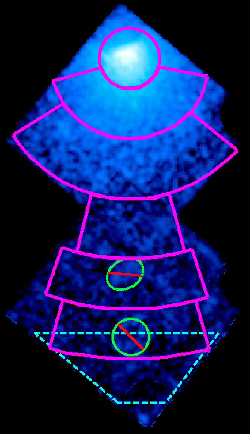
Figure 1: Mosaic XIS image of ESO 3060170 in 0.5-4.0 keV band with NXB and CXB subtracted. The image is corrected for exposure and vignetting. Pink segments represent regions extracted for spectral analysis. Small green ellipses represent excluded point sources. Cyan trapezoid represents region extracted for “offset” background spectra. [see the electronic edition of the journal for a color version of this figure.]

We observed the central and outer regions of ESO 3060170 with Suzaku in two pointings during May 2010 (PI: Y. Su). Three X-ray CCDs (XIS 0, 1 and 3) were used and the observation log is listed in Table 1. A mosaic of the XIS images in the 0.5-4.0 keV band is shown in Figure 1. This observation was taken after XIS0 was partially damaged by being flooded with large amounts of charge, which saturated the electronics and created a permanently unusable region.

Data reduction and analysis were performed with the HEASOFT 6.12 software package using CalDB 20120209. Data were obtained in both $3\times 3$ and $5\times 5$ data readout modes; $5\times 5$ mode data were converted to $3\times 3$ mode and merged with the $3\times 3$ mode data. The events were filtered by retaining those with a geomagnetic cutoff rigidity $>6$ GeV/c, and an Earth elevation $>10^{\circ}$. The calibration source regions and hot pixels were excluded. Light curves were filtered using CIAO 4.3 script lc_clean to exclude times with flares. The resulting effective exposure times are shown in Table 1. During these observations, the activity of the Solar Wind Charge eXchange (SWCX) was inferred to be low, based on data from the Advanced Composition Explorer (ACE). Stray light should be negligible since this target is not extremely bright and the two pointings were taken with a diagonal offset, which minimizes the effects of stray light (Takei et al. 2012).

2.1 Image Analysis

To produce a vignetting-corrected image, we followed standard procedure by generating flat fields based on ray-tracing the Cosmic X-ray Background (CXB) spectrum through the telescope optics. We first fit a spectral model to the CXB in a background region described in $\S 2.2$. Based on this spectrum, we used the FTOOL mkphlist to simulate $10^{8}$ photons between $0.5-4.0$ keV, representing a uniform, extended source with radius $20^{\prime}$. These simulated incident photons were used as the input to an X-ray telescope ray-tracing simulator (FTOOL xissim; Ishisaki et al. 2007) to produce a flat-field image for each chip and pointing. We used the CIAO 4.3 tool csmooth to smooth these flat fields with a Gaussian kernel (of 5 pixels) in order to increase the signal-to-noise ratio. We scaled these vignetting-corrected images by the relevant exposure times to produce exposure maps. Source images from each chip and pointing were extracted in the 0.5-4.0 keV band. A particle (non-X-ray) background (NXB) component was generated for each chip and pointing with FTOOL xisnxbgen (Tawa et al. 2008). Mosaics of the source images, NXB images, and exposure maps for each chip and pointing were cast on a common sky coordinate reference frame. The NXB component was subtracted from each cluster image on each chip; these images were then divided by their exposure maps and merged. Finally, we subtracted the CXB surface brightness from the image. The exposure-corrected, NXB- and CXB-subtracted 0.5-4.0 keV image mosaic is shown in Figure 1. Two point sources in the offset pointing, identified by eye and indicated in Figure 1, were excluded from the spectral analysis.

2.2 Spectral analysis

We extracted spectra from six truncated annular regions, indicated in Figure 1, centered on ESO 3060170 and extending south from $0^{\prime}$-$3^{\prime}$, $3^{\prime}$-$8^{\prime}$, $8^{\prime}$-$14^{\prime}$, $14^{\prime}$-$20^{\prime}$, $20^{\prime}$-$25^{\prime}$ and $25^{\prime}$-$30^{\prime}$ (regions 1–6). The FTOOL xissimarfgen was used to generate an ancillary response file (ARF) for each region and detector. To provide the appropriate photon weighting for each ARF, we used a 2-dimensional $\beta$-model surface brightness distribution extrapolated from XMM-Newton observations (Sun et al. 2004). We used the C-statistic in all our spectral analyses and accordingly grouped spectra to have at least one count per energy bin.

Redistribution matrix files (RMFs) were generated for each region and detector using the FTOOL xisrmfgen. NXB spectra were generated with the FTOOL xisnxbgen. Spectra from XIS0, 1, & 3 were simultaneously fit in spectral modeling with XSPEC v12.7.2 (Arnaud 1996). We adopted the solar abundance standard of Asplund at al. (2009) in thermal spectral models. To compare our results with those using the abundance standard of Anders & Grevesse (1989), our iron abundances should be multiplied by 0.67. Energy bands were restricted to 0.5-7.0 keV for the back-illuminated CCD (XIS1) and 0.6-7.0 keV for the front-illuminated CCDs (XIS0, XIS3), where the responses are best calibrated. Uncertainties in fitted parameters are reported at the 90% confidence level.

2.2.1 X-ray background

We used three different methods to determine the X-ray background. In the first method, called “offset” background, we use background spectra (one for each detector) extracted from a region $\sim 28^{\prime}$ south of the center (partially overlapping region 6). Since the observed surface brightness profile is flat in this background region, ARFs were generated by assuming uniform sky emission with a radius of $20^{\prime}$. We simultaneously fitted these background spectra to determine the surface brightness of Galactic components and the CXB, taking into account that there may be small amounts of emission from the group at this distance. We used XSPEC to fit each spectrum with a multi-component background model consisting of an apec thermal emission model for the Local Bubble (apec_LB), an additional apec thermal emission model (apec_MW) for the Milky Way emission in the line of sight (Smith et al. 2001), and a power law model pow_CXB (with index $\Gamma=1.41$) characterizing the CXB (De Luca & Molendi 2004). We also included a thermal apec model for any residual emission from the group (apec_ESO) in this outer region. All these components but the Local Bubble were assumed to be absorbed by foreground (Galactic) cooler gas, with the absorption characterized by the phabs model for photoelectric absorption. Photoionization cross-sections were from Balucinska-Church & McCammon (1998). We adopted a Galactic hydrogen column of $N_{H}=3.15\times 10^{20}$ cm^-2 toward ESO 3060170, deduced from the Dickey and Lockman (1990) map incorporated in the HEASARC $N_{H}$ tool. The final spectral fitting model was ${\tt apec}_{\rm LB}+{\tt phabs}\times({\tt apec}_{\rm MW}+{\tt pow_{\rm CXB}}+{\tt apec}_{\rm ESO}).$ The temperatures of the Milky Way and Local Bubble components were fixed at 0.25 keV and 0.10 keV, respectively (Kuntz & Snowden 2000).

The second method we call “local” background. We fitted the spectra of regions 2 through 6 simultaneously with the source plus background model ${\tt apec}_{\rm LB}+{\tt phabs}\times({\tt apec}_{\rm MW}+{\tt pow_{\rm CXB}}+{\tt apec}_{\rm ESO})$. We did not include region 1 because the contribution from low mass X-ray binaries (LMXBs) in the central region may be degenerate with the CXB component. X-ray background components (apec_LB, pow_CXB, apec_MW) were forced to have the same surface brightness in all regions. Group gaseous components were allowed to vary independently for each region.

The third method we label “deproj” background, which we determined through deprojected spectral fits. We performed a deprojected spectral analysis for regions 1–6 simultaneously using models described later in §2.2.3. Similar to the second method, we let the normalizations of all components, including group emission and X-ray background components (CXB, MW and LB), free to vary. X-ray background components (apec_LB, pow_CXB, apec_MW) were forced to have the same surface brightness in all regions, while group emission was allowed to vary independently in each region.

The results for the background components determined with these three methods are shown in Table 2. They are largely consistent with each other and are in line with the values determined by Yoshino et al. (2009) for 14 fields observed with Suzaku. Since our main results are obtained with deprojected spectral fits, we adopted the third method (“deproj”) to determine the X-ray backgrounds. We performed Markov chain Monte Carlo (MCMC) simulations with 40 chains, each chain having 10000 steps, for the simultaneous fitting used in the third method. With the margin command in XSPEC, we marginalized over the uncertainties of the normalizations of the X-ray background components. We obtained the probability distribution for each background component normalization to determine its mean and error (listed in the starred lines of Table 2).

2.2.2 Projected spectral analysis

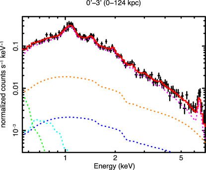
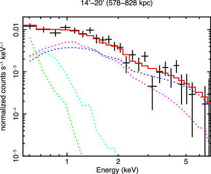
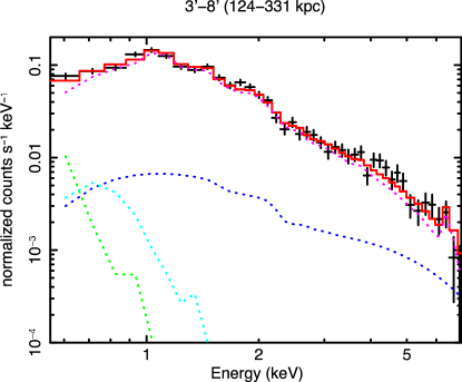
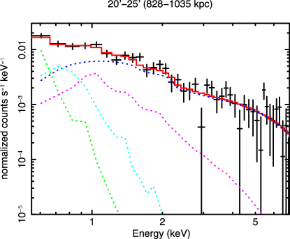
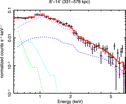
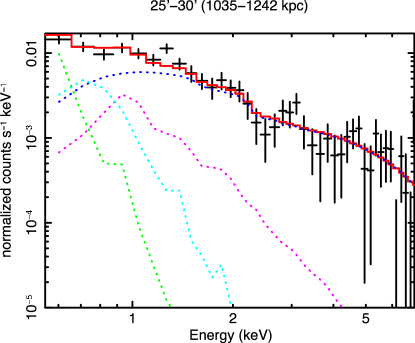
Figure 2: Suzaku XIS1 spectra for ESO 3060170 from regions 1–6. Instrumental background has been subtracted. Black: observed spectra. Red: best-fit model. Blue: CXB ($\Gamma=1.41$). Cyan: MW. Green: LB. Pink: hot gas emission. (Orange: LMXB emission for region 1). [see the electronic edition of the journal for a color version of this figure.]

We fitted the spectrum of regions 2-6 with the following model: ${\tt apec}_{\rm LB}+{\tt phabs}\times({\tt apec}_{\rm MW}+{\tt pow_{\rm CXB}}+{\tt apec}_{\rm ESO}).$ Here the apec_LB, apec_MW, and pow_CXB models represent background components discussed earlier, while the apec_ESO component represents thermal emission from group gas. For the central region 1 only, we added a power law component (pow_LMXB) with an index of 1.6 (and variable normalization) to represent unresolved LMXBs in the central galaxy (Irwin et al. 2003). ARFs derived from the $\beta$-model image were used for each region. Each background component was fixed at the surface brightness determined earlier. XIS1 spectra of regions 1–6 are shown in Figure 2. Its associated fitting results are listed in Table 3 as indicated by “projected (best-fit)”.

2.2.3 Deprojected spectral analysis

In addition to a projected spectral analysis, we also carried out a deprojected spectral analysis for regions 1–6. XSPEC v12 allows us to treat group and background emissions separately in the fitting, with different models and different ARFs: we want to deproject only the group emission and the background is more uniformly distributed than the group emission. Spectra from regions 1–6 were read into XSPEC as 6 data groups. First, we represented group emission with model projct$\times$(phabs$\times$(apec_ESO+$\tt pow_{\rm LMXB}$)); the normalization of the LMXB component is a variable fitting parameter in (the central) region 1 and was fixed at 0 for regions 2–6. The projct model performs a projection of 3-D shells into 2-D annuli with the same center. We adjusted the values of the $\beta$-model image ARFs so that they corresponded to complete (360^∘) annuli for the source regions of interest (regions 1-6). These scaled ARFs were used for the group emission (model 1). The background emission was represented by a second model: apec${}_{\rm LB}+$phabs$\times$(${\tt apec}$_MW+${\tt pow_{\rm CXB}}$), as described above. Uniform ARFs were used for the background emission (model 2). Models 1 and 2 were fitted simultaneously to the spectra. To ensure the stability of our deprojection analysis, we needed to tie the temperatures and abundances of regions 3 and 4 and, separately, the temperatures and abundances of regions 5 and 6. We first fixed the surface brightness of each background component as described earlier. The associated fitting results are listed in Table 3, labeled “deprojected (best-fit).” We next let the surface brightness of each background component freely vary in the fitting. In this way, the effects of background statistical uncertainties upon determining source properties were taken into account. For these fits we performed MCMC simulations with 40 chains, each chain having 10000 steps.

With the margin command in XSPEC, we marginalized over the uncertainties of the normalizations of all source parameters. The mean and uncertainty of each fitting parameter was derived from its probability distribution and is listed in Table 3, in the block labeled “deprojected (marginalized).” The value of each source parameter is marginalized over all other free source and background parameters. Therefore, we adopt these “deprojected (marginalized)” results as the deprojected results used for further analysis described below in §3; the alternative “deprojected (best-fit)” results are used only for testing the effects of systematic uncertainties in each background component, as will be described in §4.3.

The deprojected electron density of each spherical annulus was derived from the normalization of the ${\tt apec}_{\rm ESO}$ component in each deprojected shell obtained. The normalization of this apec model in XSPEC is proportional to the emission measure and defined as

$${\rm norm}=\frac{10^{-14}}{4\pi[D_{A}(1+z)]^{2}}\int{n_{e}n_{H}}{dV},$$

where $D_{A}$ is the angular distance to the group, and $V$ is the volume of the spherical annulus. We assume that the hot gas density has a single value in the given volume for each spherical annulus. As indicated by tests performed by Su & Irwin (2013) for NGC 720, when a single volume is divided into 10 spatial bins and analyzed separately, the sum of the gas masses of the 10 bins is within 10% of the gas mass obtained by analyzing a single integrated bin of the same volume. We did not correct for the point spread function (PSF) overlap between adjacent regions caused by the $1.5^{\prime}-2^{\prime}$ spatial resolution of Suzaku in our analysis. Humphrey et al. (2012) found that this effect was insignificant in their results for RXJ 1159+5531 and the annular widths in our work are $\sim 50\%$ larger than those of Humphrey et al. (2012), further reducing such effects.

2.3 Stellar mass estimates from infrared imaging

We will be interested in determining the radial profile of the iron mass-to-light ratio in this group. We used $K$-band imagery from the WISE (Wide-Field Infrared Survey Explorer) public archive to estimate the stellar light distribution in ESO 3060170. We analyzed three $2^{\circ}\times 2^{\circ}$ images, with one centered on ESO 3060170, one centered $2^{\circ}$ east, and one centered $2^{\circ}$ west of the group center. All three images were reduced using SExtractor to detect point sources. Point sources were excluded and replaced with a locally interpolated surface brightness using the CIAO tool dmfilth. We determined the surface brightness of the local infrared background using the average of the two offset pointings to the east and west, which were consistent with each other within 2%. We subtracted this average background surface brightness from the infrared surface brightness in each of the areas subtended by regions 1-6. We converted source counts in each region to the corresponding magnitude and corrected for Galactic extinction. We adopted a Solar $K$-band absolute magnitude of $M_{K\odot}=3.28$ (Binney & Merrifield 1998) and derived the stellar mass by adopting a stellar mass-to-light ratio of $M_{*}/L_{K}$ of 1.17 $M_{\odot}/L_{K\odot}$ (Longhetti et al. 2009).

3 Results

3.1 Temperature and density

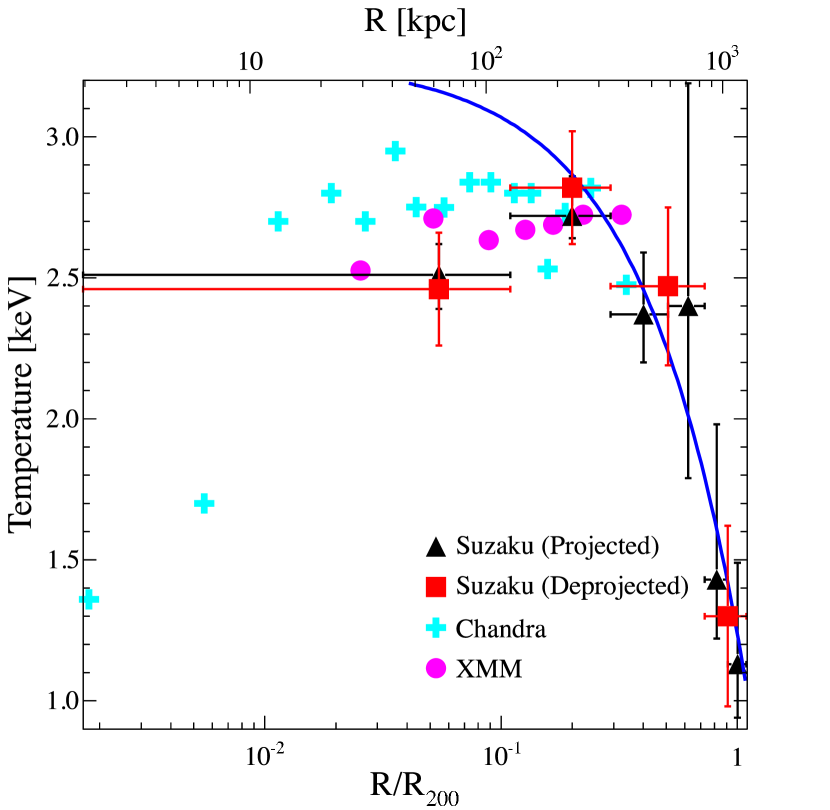
Figure 3: Radial temperature profile of ESO 3060170. Black triangles: projected temperatures. Red squares: deprojected temperatures. Blue solid line: the scaled temperature profile by Pratt et al. (2007). We adopted the deprojected results within 0.8 R₂₀₀ and the projected results beyond 0.8 R₂₀₀ as a global temperature profile. Cyan crosses: temperature profile derived with Chandra observations (Sun et al. 2004). Pink circles: temperature profile derived with XMM-Newton observations (Sun et al. 2004). The uncertainties of Chandra and XMM-Newton measurements are not shown in this plot. [see the electronic edition of the journal for a color version of this figure.]

Projected and deprojected temperature profiles are shown in Figure 3. The projected temperature profile is roughly isothermal ($\sim 2.5$ keV) within $0.8R_{200}$ (800 kpc); this is consistent with the temperature profile between 20 kpc and 400 kpc found by Sun et al. (2004) from Chandra and XMM-Newton data. The temperature drops quickly beyond 800 kpc to $1.13^{+0.36}_{-0.19}$ keV at $R_{\rm 200}$ (1.15 Mpc). This temperature drop (by a factor of $\sim 2.2$) is smaller than found on the same normalized scale in other clusters observed with Suzaku (Akamatsu at al. 2011).

Temperatures of regions 3 and 4 were linked, as were the temperatures of regions 5 and 6. The projected and deprojected temperatures of the outer two bins are consistent, so we combined the deprojected temperatures of the inner 4 bins with the projected temperatures of the outer two bins to construct a global temperature profile for further analysis. This global temperature profile is plotted in Figure 3, where it is shown to be consistent with the following heuristic formula calibrated by Pratt et al. (2007) for clusters over a radial range of $0.125<R/R_{200}<0.5$:

$$T/T_{X}=1.19-0.74~{}R/R_{200},$$

where $T_{X}$ is the peak temperature.

Higher resolution Chandra observations analyzed by Sun et al. (2004) revealed a small cool core of $1.32^{+0.08}_{-0.10}$ keV within 10 kpc (0.24^′). They also found that the gaseous cooling time $t_{c}$ is less than the Hubble time $t_{H}$ out to 70 kpc ($1.7^{\prime}$). The fact that the cool core is much smaller than the region over which $t_{c}<t_{H}$ suggests that the central regions have been heated (Sun et al. 2004). Suzaku cannot spatially resolve such a small cool core due to its relatively large PSF. Nonetheless, we looked for the signature of this cool core in a Suzaku spectrum extracted from within a central circular region of $3^{\prime}$ diameter. We fitted this central spectrum with two independently varying thermal diffuse emission components, along with the LMXB component described §2.2. The two temperatures we obtained were $1.03^{+0.63}_{-0.33}$ keV and $2.76^{+0.16}_{-0.16}$ keV, with the lower temperature component being consistent with the $1.3$ keV found by Sun et al. (2004).

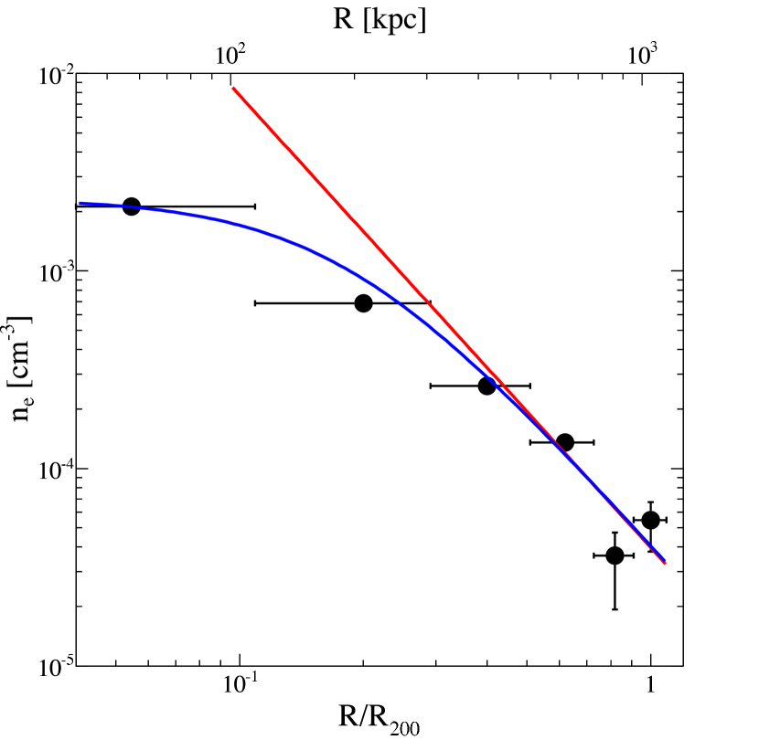
Figure 4: Black dots: deprojected electron density profile of ESO 3060170. Blue line: beta profile fit to deprojected electron density profile, $n_{e}\propto[1+(r/r_{c})^{2}]^{-3\beta/2}$, where $\beta=0.78,r_{c}$=188.68 kpc. Red line: power law fit to deprojected electron density profile, $n_{e}\propto r^{-2.29}$. [see the electronic edition of the journal for a color version of this figure.]

The deprojected electron density profile, shown in Figure 4, is derived from a combined fit for all annular regions. The profile approximately follows a power law model $n_{e}\propto r^{-\delta}$, with a best fit of $\delta=2.29\pm 1.4$. We also fit the profile to a $\beta$-model, $n_{e}=n_{e,0}[1+(r/r_{c})^{2}]^{-3\beta/2}$, obtaining a best fit of $\beta=0.78\pm 0.29$.

3.2 Entropy and pressure

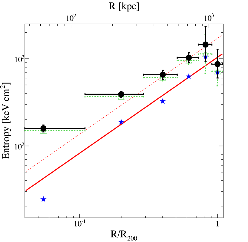
Figure 5: Black circles: radial profile of entropy ($K=n_{e}^{-2/3}kT$) in ESO 3060170. Blue stars: entropy profile corrected the variation of $f_{\rm gas}(r)$ with respect to 0.15 (Pratt et al. 2010). Green triangles: radial profile of entropy determined when background components were fixed in the fitting. Red solid line: entropy profile from simulations, $K\propto r^{1.1}$; normalization is derived from Voit et al. (2005) ($K_{\rm sim}$). Red dashed line: entropy profile from simulations, $S\propto r^{1.1}$ with normalization determined by fit to intermediate radii ($K_{\rm fit}$). [see the electronic edition of the journal for a color version of this figure.]

The entropy of gas in groups and clusters is a powerful diagnostic for investigating gaseous heating processes in such systems. Figure 5 shows the entropy ($K=n_{e}^{-2/3}kT$) profile of ESO 3060170 derived from these Suzaku observations out to $R_{200}$ (1.15 Mpc). Within $R_{500}$ (750 kpc), the best-fit power law index of this entropy profile is $0.81\pm 0.23$, which was obtained with the inner four data points. This is consistent with the average entropy profile of 31 clusters observed with XMM-Newton (Pratt et al. 2010), for which a best-fit power law index of 0.98 was found out to about $R_{500}$; the entropy profile of ESO 3060170 is also consistent with those of $\sim 20$ galaxy groups observed within $R_{500}$ by Sun et al. (2009), who found an average best-fit power law index of 0.7. If purely gravitational processes energize the gas, self-similar structure formation simulations predict that the entropy should rise with radius as $S\propto r^{1.1}$ (Voit et al. 2005). In ESO 3060170, the observed entropy profile flattens and declines beyond $\sim R_{\rm 200}$ (1.15 Mpc), regardless of which normalization was adopted for the expected entropy profile. We tested whether this behavior at large radii is an artifact of underestimating the background: as discussed in detail in §4.3, we varied each background component and found this entropy rollover to persist at large radii. A similar entropy downturn has been found in several massive clusters observed at large radii by Suzaku (Walker et al. 2012c).

We would like to compare the observed entropy profile to expectations from numerical simulations and to those of other groups and clusters. We estimated the normalization of the expected entropy profile in two different ways, as shown in Figure 5. The first estimate, $K_{\rm sim}$, is based on the simulation of gravitational structure formation derived by Voit et al. (2005):

$$K_{\rm sim}(R)=1.32~{}K_{200}(R/R_{200})^{1.1},$$

where the normalization $K_{200}$ is given by

$$K_{200}=362~{}\frac{GM_{200}\mu m_{p}}{2R_{200}}\left(\frac{1}{\rm keV}\right)\times\left[\frac{H(z)}{H_{0}}\right]^{-4/3}\left(\frac{\Omega_{m}}{0.3}\right)^{-4/3}~{}{\rm keV~{}cm^{-2}}.$$

Our second estimate for the expected entropy profile, $K_{\rm fit}$, is based on fitting the observed entropy profile of ESO 3060170 between 0.12-0.8 $R_{\rm 200}$; at these intermediate radii, the gas is likely to be virialized and relatively free from a possible central disturbance such as AGN activity. The observed entropy profile displays a more extended central excess when compared with $K_{\rm sim}$ rather than $K_{\rm fit}$; this was also found by Eckert et al. (2013) in an analogous comparison within a cluster sample. In systems with radial variations in the enclosed gas mass fraction $f_{\rm gas}(r)$, Pratt et al. (2010) suggests that the observed entropy profile should be scaled by a correction factor $[f_{\rm gas}(r)/0.15]^{2/3}$ when comparing to numerical models. We modified this scaling factor to $[f_{\rm gas}(r)/0.15]^{2/3}$, based on the new Planck result for the cosmic baryon fraction ($f_{b}=0.15$; Planck Collaboration 2013). After applying this correction factor, the scaled entropy profile (blue stars) at intermediate radii in Figure 5 becomes more consistent with $K_{\rm sim}$ (red solid line) than the original entropy profile (black stars).

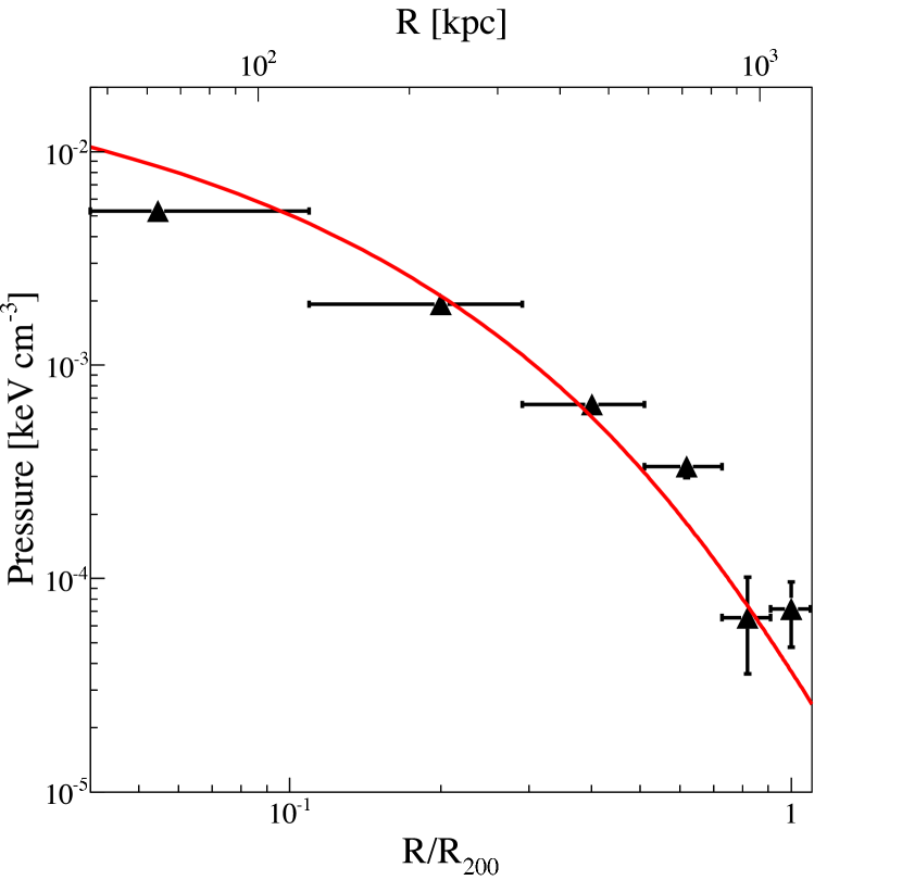
Figure 6: Black triangles: radial pressure profile of ESO 3060170. Red line: pressure profile derived by Arnaud et al. (2010). [see the electronic edition of the journal for a color version of this figure.]

The gas pressure ($P=n_{e}kT$) profile of this fossil group is shown in Figure 6 and compared to a semi-analytic universal pressure profile derived by Arnaud et al. (2010) from comparison of their numerical simulations to XMM-Newton observations of clusters. This pressure profile is characterized as

$$P(r)=P_{500}\left[\frac{M_{500}}{1.3\times 10^{14}h_{70}^{-1}M_{\odot}}\right]^{a_{p}+a^{\prime}_{p}(x)}\times\frac{P_{0}}{(c_{500}x)^{\gamma}[1+(c_{500}x)^{\alpha}]^{(\beta-\gamma)/\alpha}},$$

where

$$x=\frac{r}{R_{500}};~{}~{}~{}~{}~{}a^{\prime}_{p}(x)=0.10-(a_{p}+0.10)\frac{(x/0.5)^{3}}{[1+(x/0.5)^{3}]};$$

and $P_{500}$ and $M_{500}$ are respectively the pressure and total mass at $R_{500}$. Arnaud et al. (2010) adopted parameter values of

$$[P_{0},~{}c_{500},~{}\gamma,~{}\alpha,~{}\beta]~{}=~{}[8.403h_{70}^{-3/2},~{}1.177,~{}0.3081,~{}1.0510,~{}5.4905].$$

The observed pressure is consistent with the universal profile within 0.8$R_{200}$, while it exceeds the universal profile at large radii.

3.3 Metal abundances

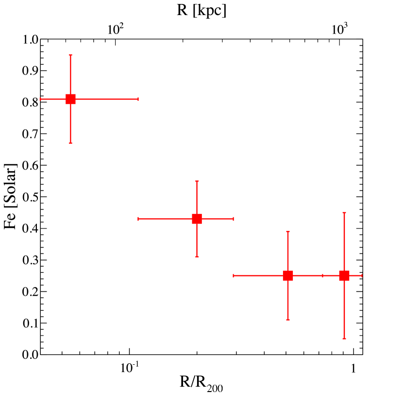
Figure 7: Deprojected radial profile of iron abundance in ESO 3060170.

The deprojected iron abundance profile for this fossil group is listed in Table 3 and shown in Figure 7. To ensure the stability of our deprojection analysis, we needed to tie the temperatures and abundances of regions 3 and 4 and, separately, the temperatures and abundances of regions 5 and 6. The best-fit iron abundance at $R_{200}$ (1.05 Mpc; 27.5^′) is $0.25\pm 0.20$ $Z_{\odot}$. Note that possibly clumpy gas would imply multi-phase thermal structure, which can lead to underestimates of the iron abundance (Buote 2002). We tested for the presence of multiphase gas in the outer parts of ESO 3060170 by fitting a spectral model with two temperature components; the fit was not improved compared to the single temperature model. However, further XSPEC analysis of synthetic two-temperature models showed that the spectrum in the outer parts is sufficiently background-dominated that it would be very difficult to separate two plausibly distinct temperature components. As indicated above, the best-fit iron abundance at $R_{200}$ is 0.25 Z_⊙ (corresponding to 0.17 Z_⊙ for Anders & Grevesse (1989) solar abundances). This is in line with previous results for massive clusters such as Virgo ($Z_{\rm Fe}\gtrsim 0.1~{}Z_{\odot}$, Urban et al. 2011), Perseus ($Z_{\rm Fe}\approx 0.3$ Z_⊙, Simionescu et al. 2011), A1689 ($Z_{\rm Fe}=0.35^{+0.65}_{-0.31}$ Z_⊙, Kawaharada et al. 2010), and A399/401 ($Z_{\rm Fe}\approx 0.2$ Z_⊙, Fujita et al. 2008). Such possibly significant iron abundance at such large radii could be indicative of early enrichment, ram-pressure stripping of infalling galaxies, or redistributed enriched gas from more central regions of the cluster.

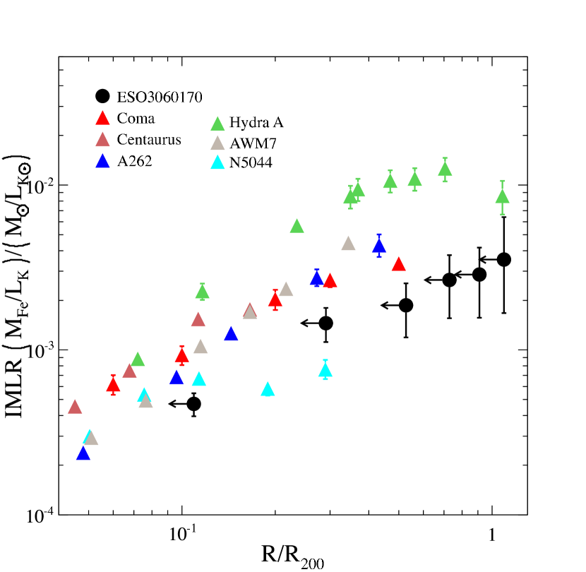
Figure 8: Profile of enclosed iron mass-to-light ratio (IMLR) in ESO 3060170 (black circles), compared to IMLR profiles of other systems (Sato et al. 2012); the radial coordinates for ESO 3060170 corresponds to the outer endpoints of radial bins. Differences in adopted solar abundance tables have been corrected for. [see the electronic edition of the journal for a color version of this figure.]

The iron-mass-to-light ratio (IMLR) tends to increase with radius in groups and clusters (Sato et al. 2012), implying that the distribution of metals is usually more extended than the galaxy light. To determine the IMLR profile in ESO 3060170, we derived the iron mass distribution from the deprojected profiles of iron abundance and gas mass (see §3.4); the stellar light distribution was derived from the $K$-band imagery described above. In Figure 8 we show the enclosed IMLR profile and compare it to several clusters. There is a large scatter among these IMLR profiles; these systems have a range of masses and temperatures and probably have different formation epochs and enrichment histories. Still, we note that the enclosed IMLR of ESO 3060170 and the NGC 5044 group are similar in their inner regions; both groups have significantly smaller IMLR values than the other plotted systems beyond $R/R_{200}\approx 0.1$, likely for different reasons. NGC 5044 is a typical galaxy group with a temperature of $\sim 1$ keV. Groups with shallower potentials may have their enriched gas redistributed out to large radii since they are more vulnerable to AGN feedback and galactic winds. In addition, galaxy groups tend to have larger stellar mass fractions than galaxy clusters, which may further reduce their IMLRs. As for ESO 3060170, fossil groups tend to have more concentrated stellar luminosity profiles than other groups, as a natural consequence of the defining characteristic of fossil groups. Thus, ESO 3060170 has a relatively smaller IMLR towards the group center. Its enclosed IMLR becomes comparable to cluster values ($>1.0\times 10^{-3}$ $M_{\odot}/L_{K\odot}$) by $R_{\rm 500}$, where IMLR $\sim 3\times 10^{-3}$ $M_{\odot}/L_{K\odot}$; this is much larger than is typical for groups, which have IMLR values ranging from $\sim 10^{-5}-10^{-3}~{}M_{\odot}/L_{K\odot}$ (Renzini 1997), although most other such groups (such as NGC 5044) have yet to be observed to their virial radii.

3.4 Mass

The temperature and density profiles were used to calculate the total mass distribution from the equation of hydrostatic equilibrium:

$$M(r)=-\frac{kT(r)r}{\mu m_{p}G}\left(\frac{{\rm d~{}ln~{}\rho_{g}(r)}}{{\rm d~{}ln}~{}r}+\frac{{\rm d~{}ln}~{}T(r)}{{\rm d~{}ln}~{}r}\right).$$

The observed global temperature profile (described in §3.1) was fitted with a three-dimensional (deprojected) temperature profile characterized by Vikhilinin et al. (2006):

$$T(r)=\frac{T_{0}(r/r_{\rm cool})^{a_{\rm cool}}+T_{\rm min}}{(r/r_{\rm cool})^{a_{\rm cool}}+1}\times\frac{(r/r_{t})^{-a}}{[1+(r/r_{t})^{b}]^{c/b}}.$$

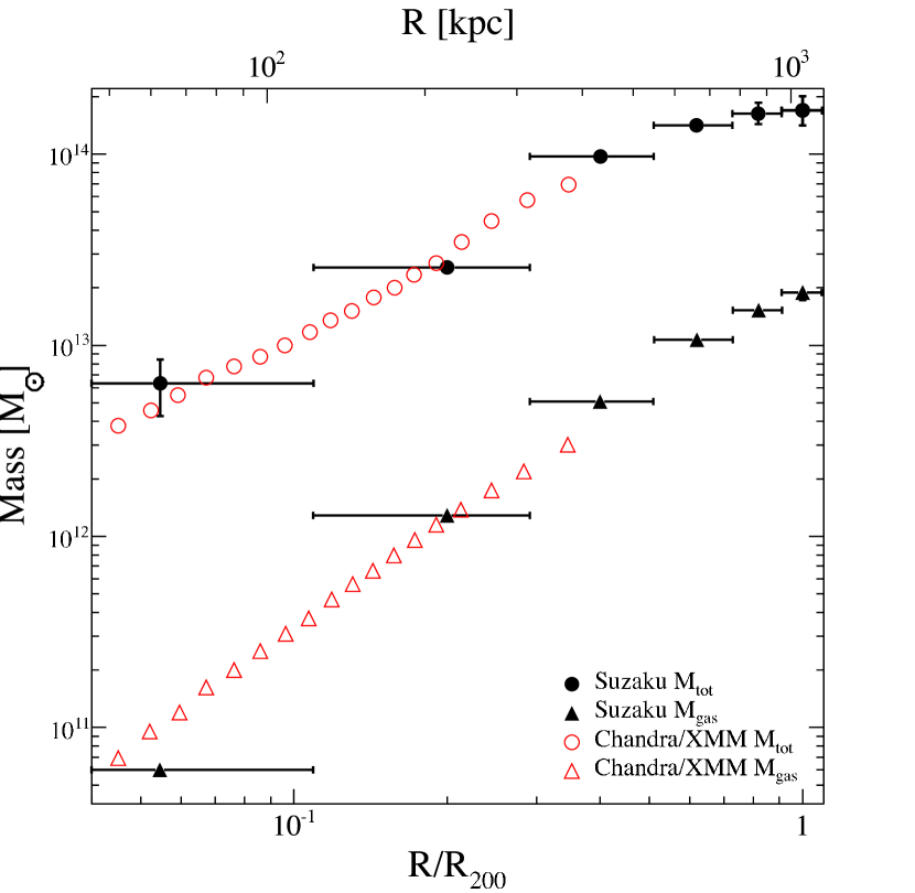
Figure 9: Black solid triangles: profile of enclosed gas mass in ESO 3060170, as derived from Suzaku data. Red open triangles: profile of enclosed gas mass in ESO 3060170, as derived from Chandra/XMM (Sun et al. 2004). Black solid circles: profile of enclosed total mass, as derived from Suzaku data. Red open circles: profile of enclosed total mass, as derived from Chandra/XMM data (Sun et al. 2004). The uncertainties of Chandra and XMM-Newton measurements are not shown in this plot. [see the electronic edition of the journal for a color version of this figure.]

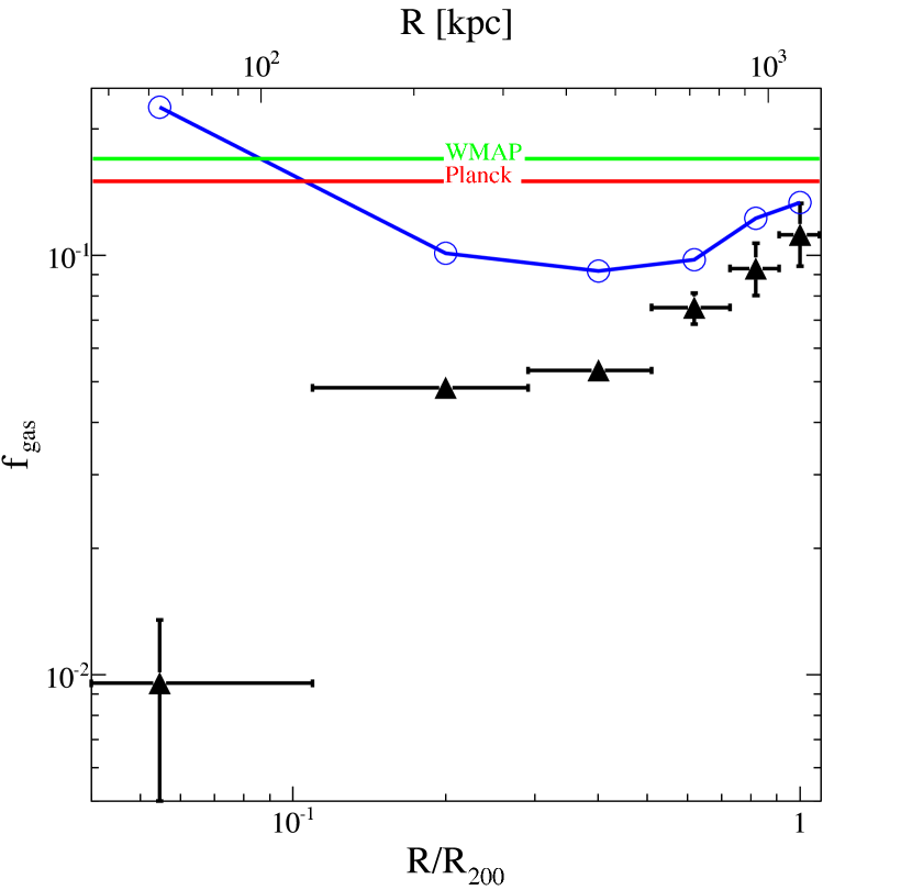
Figure 10: Black triangles: profile of enclosed gas mass fraction in ESO 3060170. Green line: baryon fraction of the universe ($f_{b}=0.17$), as determined by WMAP (Hinshaw et al. 2009). Red line: baryon fraction of the universe ($f_{b}=0.15$), as determined by Planck (Planck Collaboration, 2013). Blue: profile of enclosed baryon fraction (uncertainties are not shown).

Uncertainties in mass estimates were assessed using Monte Carlo realizations of the temperature and density profiles. Total mass and gas mass profiles are shown in Figure 9; the enclosed gas mass profile and the enclosed baryon mass fraction profile are shown in Figure 10. The total mass within $R_{\rm 200}$ (1.15 Mpc) is estimated to be $1.7\times 10^{14}M_{\odot}$; this leads to a gas mass fraction of $f_{\rm gas}=0.11^{+0.02}_{-0.02}$. Including the stellar mass contribution as described in §2.3, we obtained a baryon fraction of $f_{b}\approx 0.13^{+0.02}_{-0.02}$, consistent with the cosmological baryon fraction $f_{b}=0.15$ (Planck Collaboration 2013) and comparable to those of some massive clusters (cf. George et al. 2009; Kawaharada et al. 2010). In Figure 9 we also plot the total mass and gas mass profiles derived by Sun et al. (2004) from Chandra and XMM-Newton observations of ESO 3060170 within 450 kpc; our results are consistent within the regions of overlap. Our total mass is also in line with the extrapolation by Sun et al. (2004) to $R_{\rm vir}$.

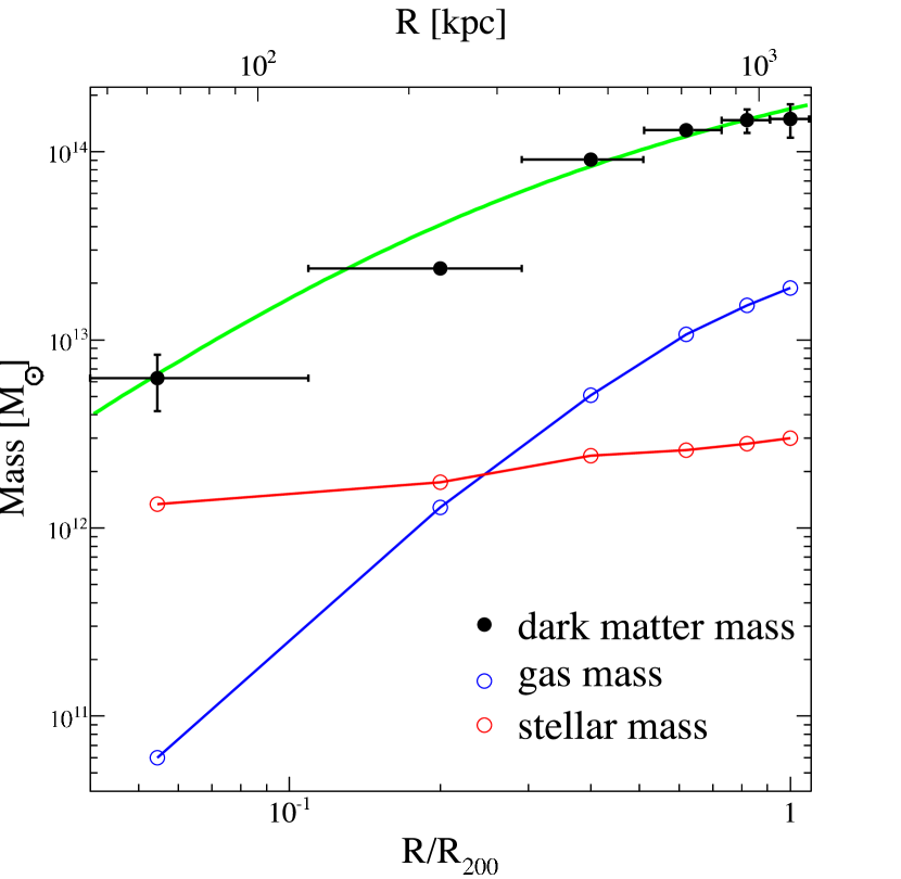
Figure 11: Black circles: enclosed dark matter mass profile of ESO 3060170. Green line: best-fit NFW dark matter mass profile, with concentration $c=6.4\pm 4.2$ and scaling radius $r_{s}=176\pm 126$ kpc. Blue (Red) line: enclosed gas (stellar) mass profile (uncertainties are not shown). [see the electronic edition of the journal for a color version of this figure.]

We obtained the dark matter distribution in this group by subtracting the baryonic mass distribution from the total mass distribution. In Figure 11 we compare the resulting dark matter mass profile to the quasi-universal dark matter mass profile of Navarro et al. (1997):

$$M(r)=4\pi\delta_{c}\rho_{c}(z){r_{s}}^{3}m(r/r_{s}),$$

where

$$m(x)={\rm ln}(1+x)-\frac{x}{1+x}$$

and the associated dark matter density profile is

$$\rho(r)=\frac{\rho_{c}(z)\delta_{c}}{(r/r_{s})(1+r/r_{s})^{2}};$$

here $r_{s}$ is a scaling radius, $\rho_{c}(z)=3H(z)^{2}/8\pi G$, and

$$\delta_{c}=\frac{200}{3}\frac{c^{3}}{{\rm ln}(1+c)-c/(1+c)},$$

from which we can determine the dark matter concentration $c$. We derived values of $c=6.9\pm 4.5$ and $r_{s}=163\pm 121$ kpc. Given the large uncertainty, such a dark matter concentration is consistent with those of non-fossil systems with similar masses and temperatures (Ettori et al. 2010). The derived virial radius $R_{\rm vir}$=1.12 Mpc ($c\equiv$ $R_{\rm vir}/r_{s}$) is nearly equal to $R_{200}$ (1.15 Mpc).

4 Discussion

4.1 Comparison of density and temperature profiles to simulations

As shown in §3.2, our Suzaku observations of ESO 3060170 indicate that its entropy ($K=n_{e}^{-2/3}kT$) profile flattens at large radii relative to the $K\propto r^{1.1}$ behavior expected from simulations. This entropy flattening has also been found in some massive clusters (cf. Walker et al. 2012c). Currently, there are several proposed explanations for such shallow entropy profiles at large radii. One suggestion is that the gas is clumpy at large radii (Simionescu et al. 2011), causing the emissivity-weighted density to be higher than the actual average density. An alternative explanation is that the ion temperature may be higher than the electron temperature in the outer parts of a cluster after relatively recent heating by an accretion shock (Hoshino et al. 2010); thus, the measured electron temperature is lower than the eventual equilibrium temperature in these regions. Yet another suggestion is due to Cavaliere et al. (2011), who propose a cluster evolutionary model incorporating the effects of the weakening of accretion shocks over time; Walker et al. (2012c) finds this latter model is consistent with the observed entropy flattening. It is also possible that more than one of these processes may be occurring.

In Figure 5 we compared the observed entropy profile (black dots) to the theoretical predictions $K_{\rm sim}$ (solid red line) from Voit et al. (2005) and in Figure 6 we compared the observed pressure profile (black dots) to the theoretical expectations of Arnaud et al. (2010). We derive similar comparisons for the gas density and temperature profiles by using the following equations for observed and theoretical quantities:

$$K_{\rm obs}\propto n_{\rm obs}^{-2/3}T_{\rm obs};~{}~{}~{}~{}P_{\rm obs}\propto n_{\rm obs}T_{\rm obs};~{}~{}~{}~{}K_{\rm th}\propto n_{\rm th}^{-2/3}T_{\rm th};~{}~{}~{}~{}P_{\rm th}\propto n_{\rm th}T_{\rm th}.$$

The following relations are equivalent:

$$\frac{n_{\rm obs}}{n_{\rm th}}=\left(\frac{P_{\rm obs}K_{\rm th}}{K_{\rm obs}P_{\rm th}}\right)^{3/5};~{}~{}~{}~{}~{}\frac{T_{\rm obs}}{T_{\rm th}}=\left(\frac{P_{\rm obs}}{P_{\rm th}}\right)^{2/5}\left(\frac{K_{\rm obs}}{K_{\rm th}}\right)^{3/5}.$$ (1)

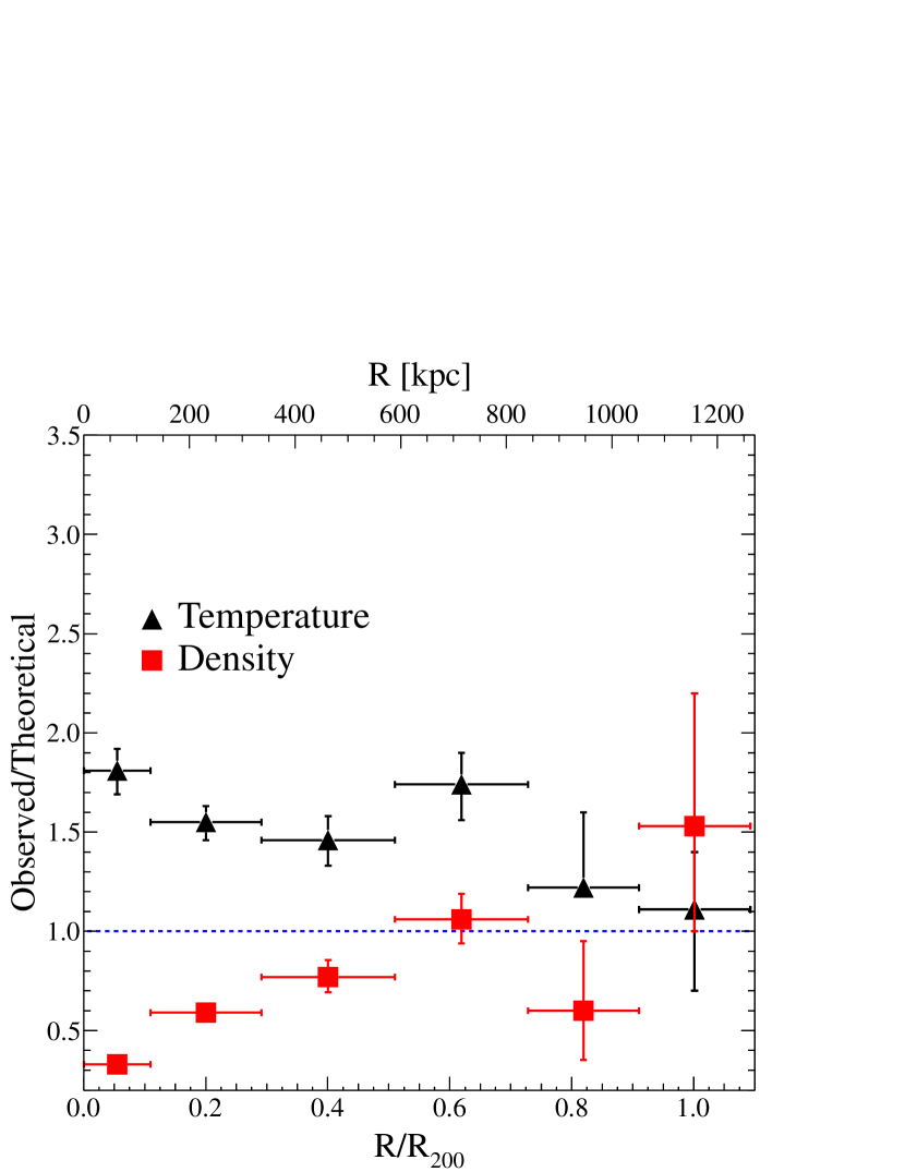
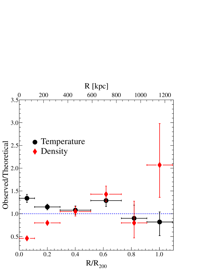
Figure 12: a) Adopting entropy profile $K_{\rm sim}$ as baseline, with normalization characterized in Voit et al. (2005). Red squares (black triangles): ratio of observed electron density (temperature) in ESO 3060170 to theoretically expected profile. Blue dotted line: Observed/Theoretical = 1. b): Adopting entropy profile $K_{\rm fit}$ as baseline, with normalization determined by fitting observed profile at intermediate radii. Red diamonds (black circles): ratio of observed electron density (temperature) to theoretically expected profile. [see the electronic edition of the journal for a color version of this figure.]

We used these relations to obtain the ratios of the observed to theoretical electron density and temperature profiles shown in Figure 12; adopted normalizations were described in $\S 3.2$.

When $K_{\rm sim}$ is adopted for the expected entropy profile, the observed temperature profile is hotter than expectations throughout (see Figure 12a). The observed density profile is lower than expectations in the central regions but is in agreement with expectations at intermediate radii; at large radii, the observed density becomes twice as large as expected (see Figure 12a). When $K_{\rm fit}$ is adopted for the expected entropy profile, the disparity between observations and theoretical expectations is smaller for the temperature profile than for the density profile (see Figure 12b). The temperature profile departs by only $\sim 20\%$ in the outer parts, while the density profile departs by more than a factor of $\gtrsim 2$. Both results imply that it is the density behavior which is driving the flattening of the entropy profile relative to theoretical expectations.

The electron density profile being shallower than theoretical expectations may be due to clumpy gas, since the emissivity scales as $\langle n^{2}\rangle$. Simulations by Nagai et al. (2011) show that gas clumpiness could cause the average density at the virial radius to be overestimated by up to a factor of 10, with 30% enhancements more likely. Suzaku observations of the Perseus cluster indicate a gas mass fraction of $f_{g}\approx 0.23$, substantially greater than the cosmic baryon fraction of $f_{b}=0.15$ (Planck Collaboration 2013), assuming the gas is smoothly distributed (Simionescu et al. 2011). If instead the gas in the outer parts of Perseus is clumpy (which enhances the X-ray emissivity for a given average gas density), the actual gas mass fraction may be less. If the true gas mass fraction in Perseus is no more than the cosmic baryon fraction, the gas density must be overestimated by a factor of 3 at its virial radius (Simionescu et al. 2011).

If the gas in the outer parts of ESO 3060170 is clumpy, the temperature may also be underestimated: in pressure equilibrium, higher density regions would have cooler temperatures and higher emissivities per unit volume than lower density regions and may dominate the emissivity-weighted temperature measures. As mentioned above, a two-temperature model for the outer regions did not provide improved fits over single-temperature models; however, the outer parts are sufficiently background-dominated that a multi-temperature model would be difficult to constrain. The enclosed gas mass fraction in this group increases smoothly with radius and never exceeds the cosmic mean. Thus, the enhancement of the gas density at large radii (relative to theoretical expectations) may not be simply a result of clumping. Instead (or additionally), the gas may have been redistributed outward due to central heating; this is also suggested by the gas density being lower than theoretical expectations within $0.5R_{\rm 200}$. Using a sample of massive clusters observed with XMM-Newton, Pratt et al. (2010) showed that clusters with entropy enhancements within $R_{500}$ (relative to theoretical expectations) had lower gas mass fractions. In simulating clusters with masses $4-11\times 10^{14}M_{\odot}$, Mathews & Guo (2011) showed that feedback energy from central black holes far exceeds radiative energy losses and causes gas to expand outward beyond the virial radii. Fossil group ESO 3060170 has a shallower gravitational potential than massive clusters, so it should be even more vulnerable to such feedback. Figure 5 shows that its entropy profile is in good agreement with $K_{\rm sim}$ (at intermediate radii) after it has been scaled downward by $[f_{\rm gas}(r)/0.15]^{2/3}$ (see §3.2); this is consistent with the effects of gas redistribution in shaping the entropy profile. Furthermore, the IMLR increases with radius in groups and clusters (Sato et al. 2012), so the metal distribution is more extended than the galaxy light, which may be a result of gas expansion.

We further address this issue quantitatively by comparing the absolute amount of gas “missing” in the central regions to the “excess” of gas in the outer regions, both relative to theoretical expectations derived from the reference entropy profiles described above. First, we obtained the theoretically expected density in each region by dividing the observed density by the observed-theoretical density ratio derived in eq.(1). Thus, we obtained the theoretically expected gas mass of each region. We next compare the “excess” gas mass in the outermost bin to its total “deficit” in the inner two bins. If we first use the best-fit entropy profile ($K_{\rm fit}$) described in §3.2 as the baseline expectation, the gas density deficiency in the central regions (red diamonds in Figure 12b) can only provide $\sim 46\%$ of the mass associated with the gas density excess at large radii. If we assume the other $\sim 54\%$ of the apparent gas mass “excess” at large radii is an artifact of clumpy gas, the true gas mass of the outermost bin is 80% of its apparently observed values. We would then obtain a total gas mass fraction of $f_{\rm gas}\approx 0.105$ after correcting for this clumpiness. This value is much smaller than the cosmological baryon fraction $f_{b}\approx 0.15$ (as well as the baryon fraction of $f_{b}\sim 0.17\pm 0.02$ found in fossil group RXJ 1159+5531 by Humphrey et al. 2012). If we instead use the entropy profile $K_{\rm sim}$ derived from simulations (Voit et al. 2005) as the baseline expectation, the gas mass “missing” in the central regions (red solid squares in Figure 12a) can account for $160\%$ of the “excess” gas mass at larger radii. In other words, gas redistribution alone would be sufficient to explain our observational results and there would be no need to invoke clumpy gas in the outer parts of this fossil group. Moreover, the “extra” 60% of gas mass in the central regions would suggest that 10% of the total gas has been driven out beyond the virial radius of this group, perhaps by central AGN activity or galactic winds; this would also be consistent with the enclosed baryon fraction of this fossil group/poor cluster being somewhat smaller than the cosmological value. Another possibility is that the 60% deficiency of gas mass in the central regions may have been consumed by star formation. Without any more knowledge such as which reference entropy profile is more appropriate to be adopted, we conservatively conclude that the flattening of the entropy profile at large radii in this fossil group may be due to a combination of multiple factors including gas clumpiness and/or gas redistribution. We note that there are large uncertainties in the gas density excesses and deficits derived from respectively adopting the $K_{\rm sim}$ and $K_{\rm fit}$ reference entropy profiles; consequently, we cannot make a statistically significant distinction between the clumpiness and redistribution scenarios.

4.2 The nature of fossil groups

The entropy profile of fossil group ESO 3060170 is observed to rise outward then roll over at $0.9R_{200}$; this is consistent with the entropy behavior in several massive clusters observed with Suzaku, but contrary to that of fossil group RXJ 1159+5531 (Humphrey et al. 2012). Most Suzaku observations of clusters have extended to only a fraction of their virial radii, therefore covering only a small fraction of the circular projected area within $R_{\rm vir}$. It has been suggested that azimuthal variations in cluster properties may be responsible for the observed scatter in Suzaku observations of cluster entropy profiles at large radii (Eckert et al. 2012; Walker et al. 2012c). Azimuthally averaged studies of massive clusters with the ROSAT and Planck satellites find entropy profiles that rise steadily with radius (Eckert et al. 2013), in contrast to the entropy rollovers found in Suzaku cluster observations with more limited azimuthal coverage. The Humphrey et al. (2012) study of fossil group RXJ 1159+5531 was also azimuthally more complete than our study of ESO 3060170, since RXJ 1159+5531 is more distant and has a smaller temperature (thus, a smaller virial radius). We would need more complete areal coverage of ESO 3060170 to test whether its entropy profile varies azimuthally. Alternatively, these disparate entropy profiles may indicate that fossil groups are rather heterogeneous, with various evolutionary histories.

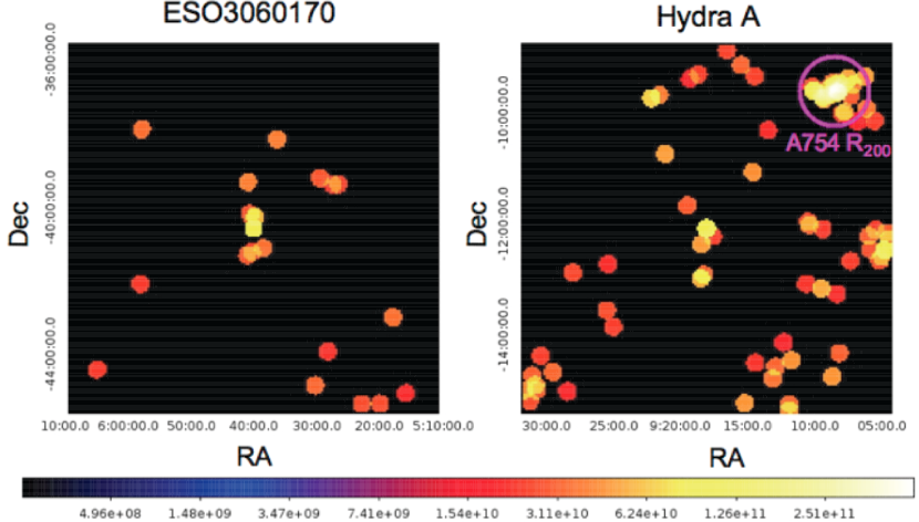
Figure 13: Maps of galaxies around ESO 3060170 (left) and Hydra A (right) on a scale of 25 Mpc, extracted from the 6dF galaxy survey. Galaxies are color-coded by their $R$-band luminosities. Pink circle: $R_{200}$ (= 2.3 Mpc) of Abell 754 (Sivakoff et al. 2008). [see the electronic edition of the journal for a color version of this figure.]

Simulations predict that fossil systems tend to reside in less dense environments than non-fossil systems with similar masses and formation epochs (Díaz-Giménez et al. 2011; D’Onghia 2005; Dariush 2007). We compared the environment of fossil group ESO 3060170 ($kT=2.8$ keV; $D_{L}$ = 154 Mpc) to that of the normal poor cluster Hydra A, which has a similar gas temperature ($kT=3.0$ keV) and a 50% larger distance ($D_{L}$ = 238 Mpc). Both systems are in the southern sky and are within the coverage of the 6dF galaxy redshift survey (Jones et al. 2009), from which we selected galaxies within a (25 Mpc)³ cube centered on each system. We only included galaxies with reliably determined redshifts and selected galaxies to the same limiting luminosity in each system. The 6dF sample is nearly complete to an $R$ magnitude of 15.6, so we selected galaxies to this magnitude limit around the more distant Hydra A system; around ESO 3060170 we selected galaxies to the equivalent limiting luminosity, corresponding to a magnitude limit 0.94 mag brighter. There are 82 such galaxies in the (25 Mpc)³ volume around Hydra A, with a total $R$-band luminosity of 2.76$\times 10^{12}$ $L_{\odot}$. There are only 20 such galaxies in the (25 Mpc)³ volume around ESO 3060170, with a total $R$-band luminosity of 6.3$\times 10^{11}$ $L_{\odot}$ (less than a quarter of that around Hydra A). In Figure 13 we show galaxy maps on a scale of 25 Mpc centered on each system. Hydra A is connected to rich cluster Abell 754 (to the northwest) by a structure described as a filament by Sato et al. (2012), while ESO 3060170 resides in a more isolated environment. A $B$-band comparison yielded similar results.

Most fossil groups have larger mass-to-light ratios than non-fossil groups at a given total mass, implying that fossil groups are optically deficient (Proctor et al. 2011). Jones et al.  (2003) noted that fossil groups with temperatures comparable to Virgo ($\sim 2$ keV) lack galaxies more luminous than $L_{*}$ (the characteristic luminosity of the Schechter luminosity function; Schechter et al. 1976), whereas the Virgo cluster contains six $L_{*}$ galaxies (Jones et al.  2003). ESO 3060170 is also optically deficient ($M/L_{R}\sim 230~{}M_{\odot}/L_{R\odot}$), as is typical of fossil groups (Figure 4 in Proctor et al. 2011). This may be a consequence of relatively inefficient star/galaxy formation.

4.3 Systematic uncertainties

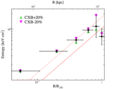
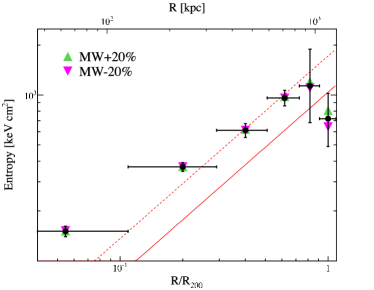
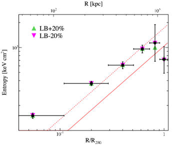
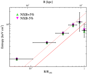
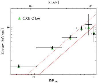
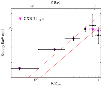
Figure 14: Black circles: entropy profile ($K=n_{e}^{-2/3}kT$) of ESO 3060170 determined when the background components were fixed in the fitting. Red solid (dashed) line: theoretical entropy profile $\propto r^{1.1}$ with normalization determined from simulations (fitting). top four figures: green (pink) triangles are entropy profiles after increasing (decreasing) the levels of the CXB, MW, LB, and NXB background components, respectively. bottom two figures: green (pink) triangles are entropy profiles after using two broken power laws for CXB modeling and adopting the low (high) marginalized value for the normalization of the bright AGN component. [see the electronic edition of the journal for a color version of this figure.]

We presented Suzaku observations of the hot gas in fossil group ESO 3060170 out to its virial radius. While there are numerous X-ray studies of massive clusters to their virial radii (cited in §1), there are relatively few studies of groups to such radii. This is largely due to the relatively low X-ray surface brightness of groups, which also makes them more vulnerable to systematic uncertainties. In order to explore how systematic uncertainties in the background can affect our results and conclusions, we varied the adopted surface brightness of each component of the X-ray background (CXB, MW, LB) by $\pm$20% and we varied the count rate of the particle background (NXB) by $\pm$5% in successive deprojected spectral fits adopting fixed background components. The effects of these background variations on the entropy profile are shown in Figure 14. The derived entropy profile at large radii, its rollover in particular, is robust against these various systematic uncertainties. The impact of these background variations on our results in the outermost region are shown in Table 4: for comparison, we first list the marginalized values for gas properties (as well as enclosed mass, gas mass fraction, and dark matter concentration) derived from fits with freely varying background components (in the row labeled “Marginalized”); we next list the best-fit values derived from fits adopting fixed background components (in the row labeled “best-fit”); these latter fitting results with fixed background components are the baseline for the systematic background variations explored in the remainder of Table 4. For each background variation, the rest of Table 4 lists how these derived quantities differ from those of the initial best-fit model. It is worth noting that we assume that each X-ray background component has the same surface brightness in all regions, which is a conventional assumption but may not be the case. The surface brightness fluctuations of unresolved cosmic point sources in the 0.5-2.0 keV band are expected to be $\sigma_{B}=3.9\times 10^{-12}\Omega^{-1/2}_{0.01}$erg s^-1 cm^-2 deg^-2 (where $\Omega_{0.01}$ is the solid angle of the target region in units of 0.01 deg²; Bautz et al. 2009); this implies that the surface brightness fluctuations of unresolved point sources would be $\sim 5\times 10^{-14}$ erg s^-1cm^-2 in the outermost region. To constrain such CXB variations is beyond the ability of current Suzaku observations. In addition, there are many other systematic uncertainties such as solar wind charge exchange, stray light, PSF, stellar mass, distance, etc. that we have not explored in our study. Humphrey et al. (2012) shows that these latter effects are relatively secondary for their Suzaku observation of RXJ 1159+5531. ESO 3060170 is closer and more massive than RXJ 1159+5531, so our results should be even less sensitive to these secondary factors.

Inspection of Table 4 and Figure 14 shows that variations in the CXB component produce the largest changes in our outermost entropy value (by $14-24$%). Consequently, we explored the systematic uncertainties associated with the CXB modeling itself. As described in §2.2.1, we adopted a single power law model for the CXB ($\Gamma=1.41$; De Luca & Molendi 2004) in our spectral analysis. Alternatively, we considered another commonly used model for the CXB (Yoshino et al. 2009) consisting of two broken power laws (Smith et al. 2007). These two components represent the integrated spectra of bright and faint AGNs separately. The bright AGNs were modeled with a photon index of $\Gamma=1.4$ above a break energy of 1.2 keV, steepening to $\Gamma=1.96$ for energies below 1.2 keV; its normalization was allowed to vary (but was constrained to be less than 4.90 photons s^-1 cm^-2 sr^-1 at 1 keV; Smith et al. 2007). Faint AGNs were also modeled with $\Gamma=1.4$ above a break energy of 1.2 keV, but steepening to $\Gamma=1.54$ for energies below 1.2 keV. This flatter power law has been well determined by many observations. The integrated spectrum of faint AGNs has smaller statistical fluctuations, so its normalization was fixed (at 5.70 photons s^-1 cm^-2 sr^-1 at 1 keV; Smith et al. 2007; Yoshino et al. 2009). We adopted this dual broken power law model (bknpow_bright+bknpow_faint) instead of the prior single power law model (pow_CXB, $\Gamma=1.41$) for the CXB and repeated the background determination and deprojected spectral analysis described in §2.2. The best-fit results for this background determination are listed in Table 2 (labeled “Fitting CXB-2”). When we marginalized over the uncertainties in the bright AGN normalization, we found two peaks in its probability distribution (see Figure 15). The normalizations associated with both peaks are within the scatter of those measured by Yoshino et al. (2009) in their analysis of 14 Suzaku background fields, so we adopted each, in turn, and repeated our spectral analysis. We list in Table 2 the normalization (and associated surface brightness) determined by this marginalization for each background component, including each of the two marginalized values found for the bright AGN component (labeled “CXB-2 low” and “CXB-2 high”). We list in Table 4 the effects on our results after adopting each of the two bright AGN normalizations, in turn (lines labeled “CXB-2 low” and “CXB-2 high”); we plot their associated entropy profiles in Figure 14 (with the same labels). These results are largely in line with our prior results, although Table 4 shows that adopting the higher bright AGN normalization (CXB-2 high) leads to a somewhat smaller gas density at large radii. Since these data are background-dominated near the virial radius, we are not able to vary the normalizations of both broken power law components in order to fully constrain this CXB model.

5 Summary

We observed the X-ray brightest fossil group ESO 3060170 with Suzaku out to $R_{200}$ (1.15 Mpc or $27.5^{\prime}$). The gas and baryon mass fractions in this group are larger than typical for groups observed within $R_{\rm 500}$, but comparable to cluster values. This observation suggests that the discrepancy between groups and clusters in their gas and baryon mass fractions will be reduced if groups are observed to sufficiently large radii. The integrated iron-mass-to-light ratio of this group is also larger than is typical for groups and comparable to cluster values. The entropy profile within $R_{500}$ (750 kpc) rises outward as $r^{1.1}$, in agreement with theoretical simulations incorporating purely gravitational processes. However, at larger radii, in the vicinity of $0.9R_{\rm 200}$, the entropy profile flattens and starts to decline outward. This flattening is primarily due to the gas density profile being shallower than theoretical expectations, possibly due to a combination of gas clumpiness and outward redistribution. This group has a high mass-to-light ratio, thus is optically deficient, as is typical for fossil groups. This may be a consequence of relatively inefficient star/galaxy formation, as perhaps indicated by a galaxy luminosity surface density map of the neighborhood within 25 Mpc of ESO 3060170. Our results are largely robust against plausible variations in the adopted background components. Further observations of groups at and beyond their virial radii are needed to more clearly establish the relationship between clusters and groups in the local Universe.

6 Acknowledgments

We would like to thank Liyi Gu, Jimmy Irwin, Evan Million, and Ka-Wah Wong for useful discussions and suggestions. We thank Kyoko Matsushita for providing data for Figure 8. Y.S. wishes to thank Steve Allen for hospitality during her visit to Stanford University. We gratefully acknowledge partial support from NASA Suzaku grant NNX10AR33G. Y.S. has been partially supported by a University of Alabama Graduate Council Research Fellowship.

Table 1: Observation log

Name	Obs ID	Effective Exposure	R.A.	Dec.	Dectectors
Center	805075010	27 ksec	05h 40m 07.20s	-40d 57m 36.0s	XIS0,1,3
$17^{\prime}$ Offset	805075060	70 ksec	05h 40m 07.20s	-41d 15m 00.0s	XIS0,1,3

Table 2: X-ray background determinations

	Cosmic		Milky Way		Local Bubble
Method	$S_{\rm CXB}^{a}$	Normb	$S_{\rm MW}^{c}$	Normd	$S_{\rm LB}^{c}$	Normd	$C/$d.o.f
Offset	$14.4^{+1.3}_{-1.0}$	$6.3^{+0.6}_{-0.4}$	$9.7^{+2.8}_{-2.8}$	$5.8^{+1.7}_{-1.7}$	$7.7^{+1.2}_{-1.2}$	$43.2^{+6.8}_{-6.5}$	2484/3019
Local	$14.8^{+1.1}_{-1.1}$	$6.5^{+0.5}_{-0.5}$	$9.1^{+1.9}_{-1.8}$	$5.4^{+1.1}_{-1.1}$	$15.3^{+2.4}_{-2.4}$	$83.2^{+12.9}_{-12.7}$	12764/14580
Deproj	$14.8^{+1.2}_{-1.1}$	$6.5^{+0.5}_{-0.5}$	$8.6^{+2.3}_{-2.3}$	$5.2^{+1.4}_{-1.4}$	$15.6^{+2.5}_{-2.4}$	$84.8^{+13.5}_{-12.8}$	16267/18350
Deproj ∗	$14.8^{+1.6}_{-1.6}$	$6.5^{+0.7}_{-0.7}$	$9.0^{+2.9}_{-2.9}$	$5.4^{+1.7}_{-1.7}$	$15.0^{+3.3}_{-3.3}$	$81.5^{+17.9}_{-17.9}$
Fitting CXB-2	${15.7^{+16.3}_{-4.2}}^{e}$	${1.3^{+1.3}_{-0.3}}^{f}$	$7.8^{+3.1}_{-5.4}$	$4.7^{+1.9}_{-3.2}$	$15.3^{+2.1}_{-7.8}$	$83.3^{+11.5}_{-42.5}$	16266/18350
CXB-2 low∗	${21.3^{+9.3}_{-9.3}}^{e}$	${1.6^{+0.7}_{-0.7}}^{f}$	$\Big{\}}$$9.1^{+2.8}_{-2.8}$	$\Big{\}}$$5.5^{+1.7}_{-1.7}$	$\Big{\}}$$14.6^{+3.4}_{-3.4}$	$\Big{\}}$$79.6^{+18.4}_{-18.4}$
CXB-2 high∗	${{31.9}^{+4.0}_{-4.0}}^{e}$	${2.4^{+0.3}_{-0.3}}^{f}$

Table 3: Summary of fit parameters for group emission in regions 1-6

Method	Annuli	Temperature	Fe	$\rm Norm^{a}$	${S_{X}}^{b}$	$C$/d.o.f
	(arcmin)	(keV)	($Z_{\odot}$)
projected	0–3	$2.51^{+0.11}_{-0.12}$	$0.69^{+0.08}_{-0.07}$	$2037.04^{+129.63}_{-120.37}$	$1231.48^{+78.36}_{-72.77}$	3506/3770
(best-fit)	3–8	$2.72^{+0.14}_{-0.08}$	$0.39^{+0.08}_{-0.07}$	$425.93^{+18.52}_{-18.52}$	$228.70^{+9.94}_{-9.94}$00	3341/3669
	8–14	$2.37^{+0.22}_{-0.17}$	$0.25^{+0.12}_{-0.09}$	$124.08^{+9.26}_{-9.26}$00	$63.33^{+4.72}_{-4.72}$00	3075/3307
	14–20	$2.42^{+0.85}_{-0.65}$	$0.18^{+0.40}_{-0.17}$	$35.09^{+5.56}_{-7.41}$00	$17.52^{+2.78}_{-3.67}$00	1714/2082
	20–25	$1.43^{+0.55}_{-0.21}$	$0.34^{+1.15}_{-0.29}$	$9.81^{+2.22}_{-2.04}$00	$5.12^{+1.16}_{-1.06}$00	2454/2849
	25–30	$1.13^{+0.36}_{-0.19}$	$-$	$6.47^{+2.13}_{-1.85}$00	$3.92^{+1.29}_{-1.12}$00	2179/2676
deprojected	0–3	$2.47^{+0.14}_{-0.16}$	$0.81^{+0.13}_{-0.11}$	$1438.66^{+129.65}_{-129.65}$	$1263.01^{+113.82}_{-113.82}$	16266/18353
(best-fit)	3–8	$2.82^{+0.15}_{-0.15}$	$0.43^{+0.10}_{-0.09}$	$435.93^{+19.85}_{-19.16}$	$234.05^{+10.66}_{-10.29}$
	8–14	$\Big{\}}$$2.48^{+0.21}_{-0.20}$∗	$\Big{\}}$$0.25^{+0.13}_{-0.10}$∗	$124.32^{+11.12}_{-10.55}$	$64.16^{+5.74}_{-5.44}$00
	14–20			$49.26^{+8.12}_{-7.75}$00	$17.77^{+2.93}_{-2.80}$00
	20–25	$\Big{\}}$$1.27^{+0.24}_{-0.21}$∗	$\Big{\}}$$0.31^{+0.44}_{-0.20}$∗	$7.51^{+5.86}_{-5.69}$00	$5.22^{+4.07}_{-3.95}$00
	25–30			$17.79^{+4.93}_{-4.79}$00	$3.89^{+1.08}_{-1.05}$00
deprojected	0–3	$2.46\pm 0.20$	$0.81\pm 0.14$	$1421.94\pm 150.56$	$1248.41\pm 132.18$	16266/18350
(marginalized)	3–8	$2.82\pm 0.20$	$0.43\pm 0.12$	$437.99\pm 24.64$	$235.16\pm 13.22$
	8–14	$\Big{\}}$$2.47\pm 0.28$∗	$\Big{\}}$$0.25\pm 0.14$∗	$122.71\pm 13.69$	$63.28\pm 7.06$00
	14–20			$49.82\pm 10.33$00	$17.97\pm 3.73$00
	20–25	$\Big{\}}$$1.30\pm 0.32$∗	$\Big{\}}$$0.25\pm 0.20$∗	$4.68\pm 4.18$00	$3.26\pm 2.91$00
	25–30			$13.14\pm 9.58$00	$2.88\pm 2.09$00

Table 4: Summary of Systematic Uncertainties

Tests	$n_{\rm e}$	T	Entropy	Pressure	Mass	$f_{\rm gas}$	$c$
	($10^{-5}$ cm-3)	(keV)	(keV cm2)	($10^{-5}$ keV cm-3)	(1014 M⊙)
Marginalizeda	$5.48^{+1.72}_{-2.63}$	$1.13^{+0.36}_{-0.19}$∗	$866^{+414}_{-265}$	$6.20^{+2.90}_{-2.80}$	$1.69^{+0.30}_{-0.30}$	$0.11^{+0.02}_{-0.02}$	$6.9\pm 4.5$
best-fitb	$6.38^{+1.69}_{-1.65}$		$710^{+305}_{-230}$	$7.21^{+2.42}_{-2.44}$	$1.69^{+0.30}_{-0.26}$	$0.12^{+0.02}_{-0.02}$	$6.4\pm 3.2$
CXB $+$20%	$-2.92$	$-0.20$	$+168$	$-3.99$	$-0.39$	$+0.02$	$+3.4$
CXB $-$20%	$+2.30$	$+0.45$	0$+99$	$+6.49$	$+0.27$	$-0.01$	$-2.0$
MW $~{}+$20%	$-0.48$	$+0.09$	0$+88$	$-0.01$	$-0.05$	$-0.001$	$-0.1$
MW $~{}-$20%	$+1.50$	$-0.09$	0$-66$	$-0.42$	$-0.18$	$+0.01$	$+0.8$
LB $~{}~{}~{}+$20%	$-0.23$	$+0.03$	0$+37$	$-0.08$	$-0.08$	$+0.003$	$+0.5$
LB $~{}~{}~{}-$20%	$-0.06$	$-0.01$	00$-2$	$-0.13$	$-0.12$	$+0.007$	$+0.5$
NXB $~{}~{}+$5%	$+0.70$	$+0.02$	0$-36$	$+0.93$	$-0.13$	$+0.01$	$+0.7$
NXB $~{}~{}-$5%	$-0.70$	$-0.03$	0$+36$	$-0.97$	$-0.11$	$+0.005$	$+0.5$
CXB-2 low∗∗	$-0.98$	$-0.04$	0$+53$	$-1.32$	$-0.14$	$+0.008$	$+1.0$
CXB-2 high∗∗	$-2.90$	$-0.20$	$+116$	$-0.97$	$-0.40$	$+0.02$	$+3.6$

Figure 15: The double-peaked probability distribution for the bright AGN component ($\Gamma_{1}=1.96$ for $E<1.2$ keV; $\Gamma_{2}=1.4$ for $E>1.2$ keV). The normalization of the faint AGN broken power law component is fixed when two broken power laws are used to respectively model the faint and bright AGN components of the CXB.

References

- (1) Akamatsu, H., Hoshino, A., Ishisaki, Y., et al. 2011, PASJ, 63, 1019
- (2) Anders, E. & Grevesse, N. 1989, GeCoA, 53, 197
- (3) Arnaud, K. A. 1996, ASPC, 99, 409
- (4) Arnaud, M., Pratt, G. W., Piffaretti, R., et al. 2010, A&A, 517, 92
- (5) Asplund, M., Grevesse, N., Sauval, A. J., & Scott, P. 2009, ARA&A, 47, 481
- (6) Bautz, M. W., Miller, E. D., Sanders, J. S., et al. 2009, PASJ, 61, 1117
- (7) Beuing, J., Dobereiner, S., Bohringer, H., & Bender, R. 1999, MNRAS, 302, 209
- (8) Binney, J. & Merrifield, M. 1998, Galactic Astronomy, Princeton University Press, p.53
- (9) Buote, D. A. 2002, ApJ, 574, L135
- (10) Cavaliere, L., Lapi, A., & Fusco-Femiano, R. 2011, ApJ, 742, 19
- (11) Dai, X., Bregman, J. N., Kochanek, C. S., & Rasia, E. 2010, ApJ, 719, 119
- (12) Dariush, A., Khosroshahi, H. G., Ponman, T. J., et al. 2007, MNRAS, 382, 433
- (13) De Luca, A. & Molendi, S. 2004, A&A, 419, 837
- (14) Díaz-Giménez, E., Zandivarez, A., Proctor, R., et al. 2011, A&A, 527, 129
- (15) Dickey, J. M. & Lockman, F. J. 1990, ARA&A, 28, 215
- (16) D’Onghia, E., Sommer-Larsen, J., Romeo, A. D., et al. 2005, ApJ, 630, L109
- (17) Dupke, R. A., Miller, E., de Oliveria, C. M., et al. 2010, HiA, 15, 287
- (18) Eckert, D., Molendi, S., & Vazza, F., et al. 2013, A&A, 551, 22
- (19) Ettori, S., Gastaldello, F., Leccardi, A., et al. 2010, A&A, 524, 68
- (20) Fujita, Y., Tawa, N., Hayashida, K., et al. 2008, PASJ, 60, 343
- (21) George, M., Fabian, A. C., Sanders, J. S., et al. 2009, MNRAS, 395, 657
- (22) Giocoli, C., Tormen, G., & Sheth, R. K. 2012, MNRAS, 422, 185
- (23) Hinshaw, G., Weiland, J. L., Hill, R. S., et al. 2009, ApJS, 180, 225
- (24) Hoshino, A., Henry, J. P., Sato, K., et al. 2010, PASJ, 62, 371
- (25) Humphrey, P. J., Buote, D. A., Brighenti, F., et al. 2012, ApJ, 748, 11
- (26) Irwin, J. A., Athey, A. E., & Bregman, J. N. 2003, ApJ, 587, 356
- (27) Ishisaki, Y., Maeda, Y., Fujimoto, R., et al. 2007, PASJ, 59, 113
- (28) Jones, L. R., Ponman, T. J., Horton, A., et al. 2003, MNRAS, 343, 627
- (29) Jones, D. H., Read, M. A., Saunders, W., et al. 2009, MNRAS, 399, 683
- (30) Kawaharada, M., Okabe, N., Umetsu, K., et al. 2010, ApJ, 714, 423
- (31) Khosroshahi, H., Ponman, T., & Jones, L. 2007, MNRAS, 377, 595
- (32) Kuntz, D. & Snowden, L. 2000, ApJ, 543, 195
- (33) Longhetti, M. & Saracco, P. 2009, MNRAS, 394, 774
- (34) Mathews, W. G. & Guo, F. 2011, ApJ, 738, 155
- (35) Miller, E. D., Rykoff, E. S., Dupke, R. A., et al. 2012, ApJ, 747, 94
- (36) Mulchaey, J. & Zabludoff, A. 1999, ApJ, 514, 133
- (37) Nagai, D. & Lau, E. T. 2011, ApJ, 731, L10
- (38) Navarro, J. F., Frenk, C. S., & White, S. D. M. 1997, ApJ, 490, 493
- (39) Planck Collaboration, arXiv:1303.5076v1[astro-ph.CO]
- (40) Pratt, G. W., Bohringer, H., Croston, J. H., et al. 2007, A&A, 461, 71
- (41) Pratt, G. W., Arnaud, M., Piffaretti, R., et al. 2010, A&A, 511, 85
- (42) Proctor, R. N., de Oliveiria, C. M., Dupke, R., et al. 2011, MNRAS, 418, 2054
- (43) Reiprich, T., Hudson, D., & Zhang, Y., et al. 2009, A&A, 501, 899
- (44) Renzini, A. 1997, ApJ, 488, 35
- (45) Sato, T., Sasaki, T., Matsushita, K., et al. 2012, PASJ, 64, 95
- (46) Schechter, P. L. & Peebles, P. J. E. 1976, ApJ, 209, 670
- (47) Simionescu, A., Allen, S. W., Mantz, A., et al. 2011, Sci, 331, 1576
- (48) Sivakoff, G., Martin, P., Zabludoff, A., et al. 2008, ApJ, 682, 803
- (49) Smith, R. K., Brickhouse, N. S., Liedahl, D. A., & Raymond, J. C. 2001, ApJ, 556, L91
- (50) Smith, R. K., Bautz, M. W., Edgar, R. J., et al. 2007, PASJ, 59, 141
- (51) Su, Y. & Irwin, J. 2013, ApJ, 766, 61
- (52) Sun, M., Forman, W., Vikhlinin, A., et al. 2003, ApJ, 598, 250
- (53) Sun, M., Forman, W., Vikhlinin, A., et al. 2004, ApJ, 612, 805
- (54) Sun, M., Voit, G. M., Donahue, M., et al. 2009, ApJ, 693, 1142
- (55) Sun, M. 2012, NJPh, 14, 045004
- (56) Takei, Y., Akamatsu, H., Hiyama, Y., et al. 2012, AIPC, 1427, 239
- (57) Tawa, N., Hayashida, K., Nagai, M., et al. 2008, PASJ, 60, 11
- (58) Urban, O., Werner, N., Simionescu, A., et al. 2011, MNRAS, 414, 210
- (59) Vikhlinin, A., McNamara, B. R., Hornstrup, A., et al. 1999, ApJ, 520, L1
- (60) Vikhlinin, A., Kravstov, A. V., Forman, W., et al. 2006, ApJ, 640, 691
- (61) Voit, G., Kay, S., & Bryan, G. 2005, MNRAS, 364, 909
- (62) von Benda-Beckmann, A. M., D’Onghia, E., Gottlober, S., et al. 2008, MNRAS, 386, 2345
- (63) Walker, S. A., Fabian, A. C., Sanders, J. S., George, M. R., & Tawara Y. 2012, MNRAS, 422, 3503 (a)
- (64) Walker, S. A., Fabian, A. C., Sanders, J. S., & George, M. R. 2012, MNRAS, 424, 1826 (b)
- (65) Walker, S. A., Fabian, A. C., Sanders, J. S., & George, M. R. 2012, MNRAS, 427, L45 (c)
- (66) Yang, X., Mo, H., & van den Bosch, F. 2008 ApJ, 676, 248
- (67) Yoshino, T., Mitsuda, K., Yamasaki, N., et al. 2009, PASJ, 61, 805