Dynamics of a tagged monomer: Effects of elastic pinning and harmonic absorption

Abstract

We study the dynamics of a tagged monomer of a Rouse polymer for different initial configurations. In the case of free evolution, the monomer displays subdiffusive behavior with strong memory of the initial state. In presence of either elastic pinning or harmonic absorption, we show that the steady state is independent of the initial condition which however strongly affects the transient regime, resulting in non-monotonous behavior and power-law relaxation with varying exponents.

It is known that the dynamics of a mesoscopic particle embedded in a viscous fluid is Markovian, and well described by the Brownian motion. The particle mean-squared displacement (MSD) grows diffusively in time as $2Dt$, where $D$ is the diffusion coefficient. However, in a crowded environment of interacting particles, the single particle may display anomalous diffusion. Let us consider a long Rouse polymer composed of $L$ monomers connected to their nearest neighbors by harmonic springs of constants $\Gamma$, and immersed in a good solvent. Its global dynamics is Markovian, and the center-of-mass diffuses with MSD behaving as $2(D/L)t$. However, the dynamics of a single tagged monomer is non-Markovian, with the MSD subdiffusing as $\sqrt{2/(\pi\Gamma)}Db_{0}\sqrt{t}$ for times $t\ll L^{2}/\Gamma$ deGennes:1971 . Here, $b_{0}$ encodes the memory of the polymer configuration at $t=0$. In particular, if the polymer at $t=0$ is in equilibrium with the solvent, the dynamics of the tagged monomer is well described Krug:1997 ; Panja:2011 ; Taloni:2010 by a fractional Brownian motion (fBm), which generalizes the Brownian motion to the case of non-independent Gaussian increments Mandelbrot:1968 ; Kolmogorov:1940 . On the other hand, if the polymer at $t=0$ is out of equilibrium, the dynamics displays aging, in that the increments are not only correlated (as in fBm), but also drawn from a Gaussian distribution with a time-dependent variance. These non-Markovian processes are relevant for many biological phenomena, such as the unzipping of DNA Walter:2012 , translocation of polymers through nanopores Kantor:2004 ; Zoia:2009 ; Panja:2010 ; Panja:2007 , subdiffusion of macromolecules inside cells Szymanski:2009 ; Weber:2010 ; Jeon:2012 ; Allegrini:1998 and single-file diffusion Lizana:2010 .

In the above applications, often the tagged particle is subject to either pinning by an elastic spring or absorption. The first case, e.g., corresponds to employing optical tweezers to confine specific molecules in order to contrast their dynamical behavior inside the crowded environment of a cell with that outside Bertseva:2012 . The second situation arises when a reactant attached to a single monomer encounters an external reactive site fixed in space Guerin:2012 ; Guerin:2013 . Moreover, in the problems of polymer translocation and DNA unzipping, the time to translocate or unzip corresponds to the absorbing time of a one-dimensional subdiffusive Gaussian process inside a finite interval with absorbing boundaries. In general, these problems are investigated numerically either by molecular dynamics simulations or by simulation of the underlying Gaussian process Dieker ; Hartman:2013 . Recently, it has been shown that subdiffusive Gaussian dynamics can be studied by the fractional Langevin equation Jeon:2010 ; Lizana:2010 ; Panja:2010-1 . This approach has been fruitfully used in presence of elastic pinning Desposito:2006 ; Desposito:2009 ; Grebenkov:2011 , but cannot easily incorporate absorption.

In this Letter, we propose a general analytical framework to compute relevant quantities such as the MSD and the absorbing time distribution of the tagged monomer, for the case of elastic pinning and harmonic absorption. These problems are relevant for practical applications: the pinning by optical tweezers is indeed elastic, while harmonic absorption mimics well a finite interval with absorbing boundaries. Our approach naturally incorporates the initial condition of the system. In the following, we specifically consider a one-dimensional Rouse chain, and mention higher dimensions in the conclusions. Our main results, summarized in Table 1, show that while the steady state is independent of the initial condition, the transient behavior exhibits very strong memory effects: (i) If a quench in temperature is performed at $t=0$, the MSD displays a bump in time and converges to the steady state value as a power law. This behavior, predicted for both pinning and absorption, could be observed in experiments. (ii) For harmonic absorption, the absorption time distribution decays exponentially with a characteristic time which is independent of the initial condition. Hence, we expect the translocation or the unzipping time to have a distribution with exponential tails, independent of the initial condition of the system.

The Rouse chain is equivalent to the one-dimensional discrete Edwards-Wilkinson (EW) interface shown in Fig. 1 Edwards:1982 ; note . Here, $h_{i}(t)$ is the displacement of the $i$-th monomer at time $t$ with respect to the origin. The elastic energy of the system is $E_{\mathrm{el}}=(\Gamma/2)\sum_{i}(h_{i+1}-h_{i})^{2}$, where $\Gamma$ is set to unity below. Additionally, the monomers are subjected to friction (set to unity) in an overdamped regime. The dynamics of the interface is described by a set of $L$ coupled Langevin equations:

$$\frac{\partial h_{i}(t)}{\partial t}=-\frac{\partial E_{\mathrm{el}}}{\partial h_{i}}+\eta_{i}(t)=\sum_{j}\Delta_{ij}h_{j}(t)+\eta_{i}(t)\>,$$ (1)

where $\Delta$ denotes the discrete Laplacian matrix, $\{\eta_{i}(t)\}$ are independent Gaussian white noises: $\langle\eta_{i}(t)\rangle=0$, $\langle\eta_{i}(t)\eta_{j}(t^{\prime})\rangle=2T\,\delta_{i,j}\,\delta(t-t^{\prime})$, with the temperature $T$ set to unity below, and $\langle\cdots\rangle$ denoting thermal averaging.

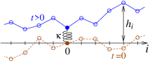
Figure 1: (Color online) Schematic of an EW interface pinned by a harmonic spring acting on the tagged monomer at $i=0$. The initial configuration $h^{0}$ (dashed) has $h_{0}^{0}=0$.

Elastic pinning.— We consider the situation where the “tagged” monomer at $i=0$ is pinned around the origin by an additional elastic force (Fig. 1). This is described by adding the term $\kappa\,h_{0}^{2}/2$ to the energy. In this case, the Langevin equations are similar to (1) with $\Delta_{ij}$ substituted by $-\Lambda_{ij}=\Delta_{ij}-\kappa\,\delta_{i,j}\delta_{i,0}$, and can be solved (cf. Supplemental Material). In order to adopt a unified formalism to deal with both pinning and absorption, we follow a Fokker-Planck approach. Let $\mathcal{W}_{t}[h|h^{0}]$ be the probability density to observe the interface in the configuration $h$ at time $t$, given that the configuration at time $t=0$ was $h^{0}$, where $h$ (respectively, $h^{0}$) denotes the vector $\{h_{i}\}$ (respectively, $\{h_{i}^{0}\}$). It obeys the Fokker-Planck equation (FPE)

$$\frac{\partial\mathcal{W}_{t}[h|h^{0}]}{\partial t}=\Big{[}\sum_{i}\frac{\partial^{2}}{\partial h_{i}^{2}}+\sum_{i,j}\frac{\partial}{\partial h_{i}}\Lambda_{ij}h_{j}\Big{]}\mathcal{W}_{t}[h|h^{0}]\>,$$ (2)

which is a $L$-dimensional generalization of the FPE for the one-dimensional Ornstein-Uhlenbeck process Risken:1989 ; Gardiner:1989 . Equation (2) can be solved through a mapping onto the imaginary time Schrödinger equation for $L$ coupled quantum harmonic oscillators (see Supplemental Material) :

$$\mathcal{W}_{t}[h|h^{0}]=\sqrt{\det\left(\frac{\Lambda}{2\pi(1-e^{-2\Lambda t})}\right)}$$ (3)

$$\times\exp\Big{[}-\frac{1}{2}(h-e^{-\Lambda t}h^{0})^{\mathrm{T}}\frac{\Lambda}{1-e^{-2\Lambda t}}(h-e^{-\Lambda t}h^{0})\Big{]},$$

where the superscript ”$\mathrm{T}$” denotes transpose operation. Note that replacing the matrix $\Lambda$ in Eq. (3) by the spring constant $\lambda$, we recover the well-known Ornstein-Uhlenbeck result for the dynamics of a particle submitted to a harmonic force.

Since Eq. (3) has a Gaussian form, all statistical information about the dynamics of the tagged monomer are encoded in the first two moments of $\mathcal{W}_{t}[h|h^{0}]$, which are conveniently obtained by introducing the local field $b=\{b_{i}\}$ acting on individual monomers. We consider the generating function

$$\mathcal{G}_{t}[b]=\int\prod_{i}dh_{i}\>e^{\sum_{i}b_{i}h_{i}}\,\mathcal{W}_{t}[h|h^{0}]\>.$$ (4)

Using Eq. (3) in Eq. (4), changing variables $h\to h-e^{-\Lambda t}h^{0}$, and doing the Gaussian integration, we get

$$\mathcal{G}_{t}[b]=\exp\bigg{[}\frac{1}{2}b^{\mathrm{T}}\frac{1-e^{-2\Lambda t}}{\Lambda}b+b^{\mathrm{T}}e^{-\Lambda t}h_{0}\bigg{]}\>.$$ (5)

	Free evolution	Elastic pinning,	Harmonic absorption,
		Long time $t\rightarrow\infty$ behavior	Long time $t\rightarrow\infty$ behavior
Single particle	$\langle h_{0}^{2}(t)\rangle=2t$	$\langle h_{0}^{2}(t)\rangle=\frac{1}{\kappa}(1-\,e^{-2\kappa t})$	$\langle h_{0}^{2}(t)\rangle=2\mu^{-1/2}\,\tanh(t/\sqrt{\mu})$
	Brownian process		$S(t)\approx\exp(-2\,\mu^{1/2}t)$
Tagged monomer	$\overline{\langle h_{0}^{2}(t)\rangle}=\sqrt{\frac{2}{\pi}}b_{0}\,\sqrt{t}$	$\overline{\langle{h_{0}^{2}(t)}\rangle}=\frac{1}{\kappa}+\frac{c_{0}}{\kappa^{2}\sqrt{t}}+\cdots$ ;	$\overline{\langle h_{0}^{2}(t)\rangle}^{\rm abs}=a_{0}\mu^{-1/3}+O(1/t)$
$T_{0}\neq 1$	$b_{0}=1+T_{0}(\sqrt{2}-1)$	$c_{0}=\sqrt{2/\pi}(T_{0}-1)$	$S(t)\approx\exp(-a_{0}\,\mu^{2/3}\,t)$
	aging process
Tagged monomer	$\overline{\langle h_{0}^{2}(t)\rangle}=\frac{2}{\sqrt{\pi}}\sqrt{t}$	$\overline{\langle h_{0}^{2}(t)\rangle}=\frac{1}{\kappa}+\frac{c_{1}}{\kappa^{3}t}+\cdots$ ;	$\overline{\langle h_{0}^{2}(t)\rangle}^{\rm abs}=a_{0}\mu^{-1/2}+O(1/t)$
$T_{0}=1$	fBm process	$c_{1}\approx 0.0711$	$S(t)\approx\exp(-a_{0}\,\mu^{2/3}\,t)$

Table 1: Summary of our results for the MSD and the survival probability: single particle versus tagged monomer of an infinite Rouse chain. We prepare the chain in equilibrium at temperature $T_{0}$, and the overbars denote the average over the ensemble of initial configurations. At time $t=0$, the system is quenched to temperature $T=1$ and let evolve following three protocols, namely, (i) free evolution, (ii) elastic pinning acting on the tagged monomer and (iii) harmonic absorption acting on the tagged monomer. The friction constant, $\Gamma$ and $D$ are all set to unity.

Note that $\mathcal{G}_{t}[0]=1$ represents the normalization of $\mathcal{W}_{t}[h|h^{0}]$. The connected correlation functions are obtained by differentiation of $\mathcal{F}_{t}[b]=\ln\mathcal{G}_{t}[b]$. In particular, using $\langle h_{i}(t)\rangle=\partial\mathcal{F}_{t}[b]/\partial b_{i}\big{|}_{b=0}$ and $\langle h_{i}(t)h_{j}(t)\rangle_{\mathrm{c}}=\partial^{2}\mathcal{F}_{t}[b]/\partial b_{i}\partial b_{j}\big{|}_{b=0}$, we get

$$\left\langle h_{i}(t)\right\rangle=(e^{-\Lambda t}h^{0})_{i},\hskip 7.11317pt\left\langle h_{i}(t)h_{j}(t)\right\rangle_{\mathrm{c}}=\left(\frac{1-e^{-2\Lambda t}}{\Lambda}\right)_{ij}.$$ (6)

At long times, we expect from the equipartition theorem that $\langle h_{0}^{2}(t\to\infty)\rangle=1/\kappa$, independent of the number of monomers in the polymer. In the case of a single particle, the steady state value is reached exponentially fast in time (Table 1). For a long polymer, the analysis of Eq. (6) shows that the steady state value is reached with a power-law decay where the exponent depends on the initial configuration. In particular, we study an initial configuration $h^{0}$ randomly sampled from the ensemble of configurations equilibrated at temperature $T_{0}$ and conditioned on $h^{0}_{0}=0$. At equilibrium, the displacements $h_{i}^{0}$’s are Gaussian distributed as $p_{\rm eq}(h^{0})=\exp[-\frac{1}{2}(h^{0})^{\mathrm{T}}\sigma^{-1}h^{0}]/\sqrt{{\det}(2\pi\sigma)}$, where $\sigma_{ij}=\overline{h_{i}^{0}h_{j}^{0}}$ is the covariance matrix, with overbar denoting averaging with respect to $p_{\rm eq}(h^{0})$. In the limit $L\to\infty$, the equilibrated EW interface corresponds to two Brownian trajectories starting at $0$ with diffusion constant equal to $T_{0}/2$. The covariance then reads $\sigma_{ij}=T_{0}\,\theta_{\mathrm{H}}(ij)\,\mathrm{min}(|i|,|j|)$, where $\theta_{\mathrm{H}}(x)$ is the Heaviside function. On the other hand, for a finite interface with periodic boundary conditions, we have $\sigma_{ij}=T_{0}\Big{[}\mathrm{min}(i,j)-ij/L\Big{]}$, where $i,\>j\in\{0,\cdots,L-1\}$. The computation of $\langle h_{0}^{2}(t)\rangle$ for long times can be performed analytically in the limit $L\to\infty$. The details are given in the Supplemental Material. We get

$$\overline{\langle h_{0}^{2}(t)\rangle}\simeq\frac{1}{\kappa}\left[1+\frac{T_{0}-1}{\kappa}\sqrt{\frac{2}{\pi t}}-\frac{T_{0}c_{1}}{\kappa^{2}t}+\cdots\right],$$ (7)

where $c_{1}=0.0711\ldots$. We thus see that the MSD tends to the steady state value $1/\kappa$ as $1/\sqrt{t}$ if $T_{0}$ is different from unity. For $T_{0}=1$, which corresponds to the temperature of the noise for $t>0$, the relaxation to steady state is as $1/t$. Moreover, for $T_{0}>1$, the MSD has a non-monotonous behaviour in time with a bump. This behaviour may be understood as the effect of the large initial spatial fluctuations of the polymer for $T_{0}>1$ that propagate towards the tagged monomer and increase its temporal fluctuations in the transient regime. Note that the calculation in Refs. Desposito:2006 ; Desposito:2009 ; Grebenkov:2011 applies to polymers equilibrated with the solvent, while here we study the effects of different initial conditions.

Harmonic Absorption.— The FPE is

$$\frac{\partial\mathcal{W}_{t}[h|h^{0}]}{\partial t}=\Big{[}\sum_{i}\frac{\partial^{2}}{\partial h_{i}^{2}}-\sum_{i,j}\Big{(}\frac{\partial}{\partial h_{i}}\Delta_{ij}h_{j}+h_{i}A_{ij}h_{j}\Big{)}\Big{]}\mathcal{W}_{t}[h|h^{0}],$$ (8)

where the positive definite matrix $A$ describing absorption is $A_{ij}=\mu\,\delta_{i,j}\,\delta_{i,0}$, with $\mu>0$ being the absorption rate. Since the absorption probability increases quadratically with distance, the FPE (8) can be solved using the mapping to a system of coupled quantum harmonic oscillators (details in Supplemental Material). We obtain

$$\mathcal{G}_{t}[b] =\mathcal{G}_{t}[0]\,\exp\Big{[}b^{\mathrm{T}}\,\Omega_{t}^{-1}\,b+b^{\mathrm{T}}\,\Omega_{t}^{-1}Y_{t}\,h^{0}\Big{]}\>,$$ (9)

$$\mathcal{G}_{t}[0] =\sqrt{\det\left(e^{-t\Delta}Y_{t}\Omega_{t}^{-1}\right)}\exp\Big{[}-\frac{1}{2}(h^{0})^{\mathrm{T}}Q_{t}h^{0}\Big{]}\>,$$ (10)

where we have introduced the four symmetric matrices

$$K =\sqrt{\Delta^{2}+4A}\>,\hskip 11.38092pt\Omega_{t}=K\coth(Kt)-\Delta\>,$$

$$Y_{t} ={K}/{\sinh(Kt)}\>,\hskip 7.11317ptQ_{t}=(\Omega_{t}+2\Delta-Y_{t}\Omega_{t}^{-1}Y_{t})/2\>.$$

In presence of absorption, $\mathcal{W}_{t}[h|h^{0}]$ is not normalized to unity, and $\mathcal{G}_{t}[0]$ is the survival probability $S(t)$, namely, the probability that an initial configuration $h^{0}$ has not been absorbed upto time $t$ Redner:2001 ; Bray:2013 . Note that the survival probability is the cumulative of the absorbing time distribution. In the long time limit, we have $\Omega_{t}\approx K-\Delta$ and $Y_{t}\approx\exp(-Kt)$, so that the survival probability asymptotically decays as $S(t)\sim\sqrt{\mathrm{det}(e^{-(K+\Delta)t})}$. Using $\det[\exp(A)]=\exp(\mathrm{Tr}[A])$, we get

$$S(t)\underset{t\to\infty}{\sim}\exp\big{[}-t\,\mathrm{Tr}\{K+\Delta\}/2\big{]}.$$ (11)

Note that the decay rate is independent of $h^{0}$.

Alternatively, one can obtain an exact expression for $S(t)$ in terms of the tagged monomer MSD, as follows. Using $S(t)=\int\prod_{i}dh_{i}\>\mathcal{W}_{t}[h|h^{0}]$, and the FPE (8), we obtain the evolution equation $\partial_{t}S(t)=-\mu\,\langle h_{0}^{2}(t)\rangle\,S(t)$, where $\langle\cdots\rangle$ in presence of absorption involves averaging over surviving realizations only, see Eq. (14) below. Using the initial condition $S(0)=1$, the solution is

$$S(t)=\exp\left(-\mu\int_{0}^{t}d\tau\,\langle h_{0}^{2}(\tau)\rangle\right).$$ (12)

As before, the mean displacement and the connected correlation function are obtained by differentiating the generating function $\mathcal{F}_{t}[b]=\ln\mathcal{G}_{t}[b]$; one finds

$$\langle h_{i}(t)\rangle =\big{(}\Omega_{t}^{-1}Y_{t}\,h^{0}\big{)}_{i},~{}\langle h_{i}(t)h_{j}(t)\rangle_{\mathrm{c}}=2\,\big{(}\Omega_{t}^{-1}\big{)}_{ij}\>.$$ (13)

The correlation function $\langle h_{i}(t)h_{j}(t)\rangle_{\mathrm{c}}$ is independent of the initial condition $h^{0}$ and has a finite value in the long time limit, while $\langle h_{i}(t)\rangle$ vanishes in that limit. In particular, the MSD in the long time limit reaches a steady state value: $\langle h_{0}^{2}(t\to\infty)\rangle=\left(2/(K-\Delta)\right)_{00}$.

A dimensional analysis in the limit of a long polymer, $L\to\infty$, allows to deduce that $\langle h_{0}^{2}(t\to\infty)\rangle=a_{0}\mu^{-1/3}$, where $a_{0}$ is a dimensionless constant of order unity. Noting that in absence of absorption, the tagged monomer subdiffuses as $\langle h^{2}_{0}(t)\rangle\sim\sqrt{t}$, we see from the absorbing term in the FPE (8) that absorption is effective over times such that $\mu\,t^{3/2}\sim O(1)$. Thus, we have $\langle h_{0}^{2}(t)\rangle\sim\sqrt{t}\,F(\mu t^{3/2})$, where the scaling function $F(x)$ is a constant as $x\to 0$. Since $\langle h_{0}^{2}(t\to\infty)\rangle$ approaches a constant, it follows that $F(x\to\infty)\sim x^{-1/3}$, giving $\langle h_{0}^{2}(t\to\infty)\rangle=a_{0}\,\mu^{-1/3}$. Equation (12) gives $S(t)\sim\exp[-a_{0}\,\mu^{2/3}t]$ in the long time limit, independently of $h^{0}$, see Table 1.

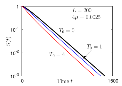
Figure 2: (Color online) Survival probability for different initial temperatures $T_{0}$. We observe at long times an exponential decay, $\overline{S(t)}\sim\exp[-a_{0}\mu^{2/3}t]$, independent of the initial condition.

We now discuss the full time evolution of $\langle h_{0}^{2}(t)\rangle$ for a given initial configuration $h^{0}$. The MSD is

$$\langle h_{0}^{2}(t)\rangle=\frac{\int\prod_{i}dh_{i}\>h_{0}^{2}\>\mathcal{W}_{t}[h|h^{0}]}{\int\prod_{i}dh_{i}\>\mathcal{W}_{t}[h|h^{0}]}\>.$$ (14)

In order to evaluate the MSD involving an average over an ensemble of initial configurations, we should weigh the contribution (14) with $p_{\rm eq}(h^{0})S(t)/\overline{S(t)}$, where $S(t)/\overline{S(t)}$ is the probability that the configurations starting from $h^{0}$ at time $t=0$ belong to the ensemble of surviving configurations at time $t$. Denoting the average MSD as $\overline{\langle h_{0}^{2}(t)\rangle}^{\rm abs}$, we compute it from the generating function

$$\ln\big{(}\,\overline{\mathcal{G}_{t}[b]}\,\big{)}=\ln\overline{S(t)}+\frac{1}{2}b^{\mathrm{T}}\,C_{t}\,b,$$ (15)

$$\overline{S(t)}=\sqrt{\frac{\det(e^{-t\Delta}Y_{t}\Omega_{t}^{-1})}{\det(\mathbf{1}+\sigma Q_{t})}},$$ (16)

$$C_{t}=2\,\Omega_{t}^{-1}+\Omega_{t}^{-1}Y_{t}\left(\mathbf{1}+\sigma Q_{t}\right)^{-1}\sigma\,Y_{t}\,\Omega_{t}^{-1},$$ (17)

with $\mathbf{1}$ the identity matrix. In particular, we obtain

$$\overline{\left\langle h_{0}^{2}(t)\right\rangle}^{\rm abs}=\partial^{2}\ln\big{(}\,\overline{\mathcal{G}_{t}[b]}\,\big{)}/\partial b_{0}^{2}\big{|}_{b=0}=\left(C_{t}\right)_{00}.$$ (18)

We compute numerically (16) and (18) for different initial temperatures $T_{0}$. The results are shown in Figs. 2 and  3. As expected by our scaling arguments, both the decay rate of $S(t)$ and the steady state value of the MSD are independent of the initial configuration. For the MSD, the approach to the steady state value $a_{0}\mu^{-1/3}$ is always as $1/t$ (inset of Fig. 3), i.e. faster than the behaviour $1/\sqrt{t}$ obtained for the case of pinning. For initially flat interface (i.e. $T_{0}=0$), we see from Fig. 3 that (18) behaves monotonically in time. While for elastic pinning, a bump appears only above $T_{0}=1$, with absorption a bump is observed already for $T_{0}=1$, and further enhanced for larger $T_{0}$ (Fig. 3). It would be interesting to understand why the approach to steady state differs in the two cases. Our numerical results are supported by direct Monte Carlo simulations of the interface dynamics, and by a careful finite-size analysis presented in the Supplemental Material.

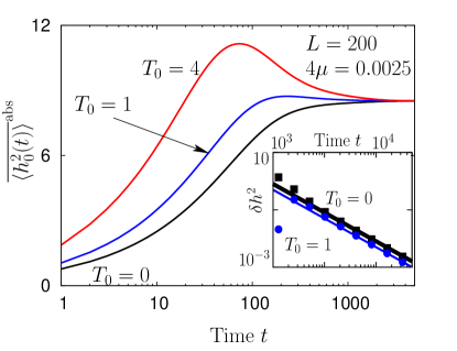
Figure 3: (Color online) MSD in presence of harmonic absorption, Eq. (18). The MSD converges to a constant which is independent of $T_{0}$. Inset : Plot of $\delta h^{2}=\big{|}\overline{\left\langle h_{0}^{2}(t)\right\rangle}^{\rm abs}-\left\langle h_{0}^{2}(\infty)\right\rangle\big{|}$ shows the $\sim 1/t$ approach to the steady state.

Conclusion.— In this paper, we analyzed tagged monomer dynamics under the action of elastic pinning or harmonic absorption. Our solution stems from the crucial observation that in presence of harmonic interactions, the stochastic evolution of the tagged monomer remains Gaussian. Some of our results, e.g., the presence of a unique steady state or the bump in MSD corresponding to a temperature quench, can be intuitively understood. Others like the exponential decay of the survival probability or the power-law transient behaviors in presence of absorption were observed in numerical simulations Kantor:2004 , but were not analytically known before. Finally, some of our results like the change of power law for $T_{0}\neq 1$ (pinning case) or the bump observed when $T_{0}=1$ (harmonic absorption) were unexpected.

In this work, we focussed on the case of one-dimensional polymers. However, it is straightforward to generalize our analysis to either a Rouse chain in $d$ dimensions Panja:2013 or a $d$-dimensional EW interface, by using the corresponding Laplacian matrix in place of $\Delta$. Moreover, hydrodynamic effects for the chain or long-range elastic interactions for the interface can also be included by replacing $\Delta$ with the corresponding fractional Laplacian $-(-\Delta)^{z/2}$ Krug:1997 ; in this case, the MSD of the tagged particle subdiffuses as $t^{(z-1)/z}$ with $z>1$ for the chain, and as $t^{(z-d)/z}$ with $z>d$ for the interface Zoia:2007 , see Supplemental Material. It would be interesting to study the effect of the pinning and absorption in the case of non-linear models such as self-avoiding polymers, and KPZ interfaces Gupta:2007 . Another open issue is to go beyond the harmonic approximation and study absorption in presence of localized targets.

Acknowledgements.— SG and AR acknowledge CEFIPRA Project 4604-3 for support. We thank M. Kardar for very helpful discussions all along this work.

Dynamics of a tagged monomer : Effects of elastic pinning and harmonic absorption –
Supplemental Material

I A. Solution of the Fokker-Planck equations

Here, we provide some details on the solution of the Fokker-Planck equations (2) and (8) of the main text.

I.1 A.1. Reminder: 1d Ornstein-Uhlenbeck process

Let us consider the Langevin equation Risken

$$\frac{\mathrm{d}x(t)}{\mathrm{d}t}=-V^{\prime}(x(t))+\eta(t),$$ (19)

describing a particle at position $x(t)$ submitted to a harmonic force $-V^{\prime}(x)=-\lambda\,x$ and a Langevin force $\eta(t)$ such that $\langle\eta(t)\rangle=0$ and $\langle\eta(t)\eta(t^{\prime})\rangle=2\,\delta(t-t^{\prime})$. The dynamics of the particle may be equivalently described by the Fokker-Planck equation

$$\frac{\partial W_{t}}{\partial t}=\frac{\partial^{2}W_{t}}{\partial x^{2}}+\frac{\partial}{\partial x}\left[V^{\prime}(x)W_{t}\right]\>,$$ (20)

where $W_{t}(x|x_{0})$ is the (conditional) probability density to find the particle at $x$ at time $t$, given that it was at $x_{0}$ at initial time. A convenient way to solve (20) is to write

$$W_{t}(x|x_{0})=Z_{t}(x|x_{0})\sqrt{\frac{P_{\mathrm{eq}}(x)}{P_{\mathrm{eq}}(x_{0})}},$$ (21)

where

$$P_{\mathrm{eq}}(x)=e^{-V(x)}=e^{-\frac{1}{2}\lambda x^{2}}$$ (22)

is the equilibrium distribution (up to a normalization). The propagator $Z_{t}(x|x_{0})$ satisfies the Schrödinger equation in imaginary time,

$$-\frac{\partial Z_{t}(x|x_{0})}{\partial t}=H_{0}\,Z_{t}(x|x_{0}),$$ (23)

where the Hamiltonian

$$H_{0} =-\frac{\partial^{2}}{\partial x^{2}}+\frac{1}{4}(V^{\prime}(x))^{2}-\frac{1}{2}V^{\prime\prime}(x)$$ (24)

$$=-\frac{\partial^{2}}{\partial x^{2}}+\frac{\lambda^{2}x^{2}}{4}-\frac{\lambda}{2}.$$ (25)

describes here a harmonic oscillator. The shift of energy $-\lambda/2$ makes the ground state energy of $H_{0}$ zero, which ensures the conservation of the probability in the diffusion problem $\int\mathrm{d}x\,W_{t}(x|x_{0})=1$. The solution of (23) corresponding to the initial condition $Z_{0}(x|x_{0})=\delta(x-x_{0})$ is well-known Feynmann-Hibbs  :

$$Z_{t}(x|x_{0})=\sqrt{\frac{\lambda\,e^{\lambda t}}{4\pi\sinh(\lambda t)}}$$ (26)

$$\times\exp\Big{[}-\frac{\lambda}{4}\Big{(}(x^{2}+x_{0}^{2})\coth(\lambda t)-\frac{2xx_{0}}{\sinh(\lambda t)}\Big{)}\Big{]}.$$

I.2 A.2. Multidimensional Ornstein-Uhlenbeck process

The Fokker-Planck equation (2) of the main text can be solved in the same manner as the one discussed in the preceding section. The probability density is

$$\mathcal{W}_{t}[h|h^{0}]=\mathcal{Z}_{t}[h|h_{0}]\sqrt{\frac{\mathcal{P}_{\mathrm{eq}}[h]}{\mathcal{P}_{\mathrm{eq}}[h^{0}]}},$$ (27)

where the equilibrium distribution now reads

$$\mathcal{P}_{\mathrm{eq}}[h]=e^{-\frac{1}{2}h^{\mathrm{T}}\Lambda h}.$$ (28)

For an interface made up of $L$ monomers, the quantum propagator $\mathcal{Z}_{t}[h|h_{0}]$ obeys a Schrödinger equation describing $L$ coupled harmonic oscillators :

$$\mathcal{H}_{0}=\Big{[}-\sum_{i}\frac{\partial^{2}}{\partial h_{i}^{2}}+\frac{1}{4}\sum_{i,j}h_{i}\,(\Lambda^{2})_{ij}\,h_{j}-\frac{1}{2}\mathrm{Tr}\{\Lambda\}\Big{]}.$$ (29)

The propagator generalizes (26), and is given by :

$$\mathcal{Z}_{t}[h|h_{0}]=\sqrt{\det\left(\frac{e^{\Lambda t}\,\Lambda}{4\pi\sinh(\Lambda t)}\right)}$$

$$\times\exp\Big{(}-\frac{1}{4}\Big{[}h^{\mathrm{T}}\,\Lambda\coth(\Lambda t)\,h+(h^{0})^{\mathrm{T}}\,\Lambda\coth(\Lambda t)\,h^{0}$$

$$\hskip 28.45274pt-h^{\mathrm{T}}\,\frac{\Lambda}{\sinh(\Lambda t)}h^{0}-(h^{0})^{\mathrm{T}}\,\frac{\Lambda}{\sinh(\Lambda t)}h\Big{]}\Big{)}.$$ (30)

Substituting the above result into Eq. (27) leads to Eq. (3) of the main text.

I.3 A.3. Harmonic absorption

The Fokker-Planck equation in the presence of absorption, Eq. (8) of the main text, can be solved using the same procedure as above. Performing the transformation (27), with $\Lambda=-\Delta$, shows that $\mathcal{Z}_{t}[h|h_{0}]$ is now the propagator for the Hamiltonian obtained by adding to (29) the term $h^{\mathrm{T}}Ah$ :

$$\mathcal{H}=\Big{[}-\sum_{i}\frac{\partial^{2}}{\partial h_{i}^{2}}+\frac{1}{4}\sum_{i,j}h_{i}\,(K^{2})_{ij}\,h_{j}-\frac{1}{2}\mathrm{Tr}\{\Delta\}\Big{]},$$ (31)

where $K^{2}=\Delta^{2}+4A$ (see main text). The propagator may be obtained along the same lines as in the previous subsection. Finally

$$\mathcal{W}_{t}[h|h^{0}]=\sqrt{\det\left(\frac{e^{-\Delta t}}{4\pi}Y_{t}\right)}\exp\Big{(}-\frac{1}{4}(h^{0})^{\mathrm{T}}Q_{t}h^{0}\Big{)}$$

$$\times\exp\Big{(}-\frac{1}{4}(h-\Omega_{t}^{-1}Y_{t}h^{0})^{\mathrm{T}}\,\Omega_{t}\,(h-\Omega_{t}^{-1}Y_{t}h^{0})\Big{)},$$ (32)

where the matrices $\Omega_{t},Y_{t}$ and $Q_{t}$ are defined in the main text.

II B. Langevin approach

We point out that in the absence of absorption, the dynamics of the line may as well be described within the Langevin approach. We can write the solution of Eq. (1) of the main text as

$$h_{i}(t)=\left(e^{-\Lambda t}\right)_{ij}h_{j}^{0}+\int_{0}^{t}\mathrm{d}\tau\,\left(e^{-\Lambda(t-\tau)}\right)_{ij}\,\eta_{j}(\tau)$$ (33)

with implicit summation over repeated indices. Averaging leads to (37). We now consider the covariance matrix

$$\left\langle h_{i}(t)h_{j}(t)\right\rangle_{\mathrm{c}}= \int_{0}^{t}\mathrm{d}\tau\int_{0}^{t}\mathrm{d}\tau^{\prime}\,\left(e^{-\Lambda(t-\tau)}\right)_{ik}\,$$

$$\times\left\langle\eta_{k}(\tau)\eta_{l}(\tau^{\prime})\right\rangle\,\left(e^{-\Lambda(t-\tau^{\prime})}\right)_{lj}$$ (34)

Using $\left\langle\eta_{k}(\tau)\eta_{l}(\tau^{\prime})\right\rangle=2\,\delta_{kl}\,\delta(\tau-\tau^{\prime})$ gives

$$\left\langle h_{i}(t)h_{j}(t)\right\rangle_{\mathrm{c}}=2\int_{0}^{t}\mathrm{d}\tau\,\left(e^{-2\Lambda(t-\tau)}\right)_{ij}$$ (35)

that leads obviously to Eq. (6) of the main text.

III C. Harmonic pinning: Derivation of Eq. (7) and its generalisation

The mean-squared displacement of the tagged monomer can be explicitly computed in the continuum limit and when the line has an infinite length. The interface height $h_{x}$ then becomes a field of a continuous variable $x$. The discrete Laplacian $\Delta$ is replaced by the Laplacian operator, so that $\Lambda_{x,x^{\prime}}\to\delta(x-x^{\prime})\Lambda_{x}$, with $\Lambda_{x}=-\Delta_{x}+\kappa\,\delta(x)$ and $\Delta_{x}=\mathrm{d}^{2}/\mathrm{d}x^{2}$. The aim of the section is to compute the variance of the tagged monomer displacement [Eq. (7) of the main text]

$$\langle h_{0}^{2}(t)\rangle_{c}=\langle\kern 1.29167pt0\kern 1.29167pt|\frac{1-e^{-2\Lambda_{x}t}}{\Lambda_{x}}|\kern 1.29167pt0\kern 1.29167pt\rangle$$ (36)

and analyse the mean displacement

$$\langle h_{0}(t)\rangle=\int\mathrm{d}x\,\langle\kern 1.29167pt0\kern 1.29167pt|e^{-\Lambda_{x}t}|\kern 1.29167ptx\kern 1.29167pt\rangle\,h_{x}^{0}$$ (37)

containing the information about the initial configuration of the line. In particular, assuming initial configurations sampled from the ensemble equilibrated at temperature $T_{0}$, leads to consider

$$\overline{\langle h_{0}(t)\rangle^{2}}=\int\mathrm{d}x\mathrm{d}x^{\prime}\,\langle\kern 1.29167pt0\kern 1.29167pt|e^{-\Lambda_{x}t}|\kern 1.29167ptx\kern 1.29167pt\rangle\,\sigma_{x,x^{\prime}}\,\langle\kern 1.29167ptx^{\prime}\kern 1.29167pt|e^{-\Lambda_{x}t}|\kern 1.29167pt0\kern 1.29167pt\rangle\>;$$ (38)

the covariance matrix for the infinite line is: $\sigma_{x,x^{\prime}}=\overline{h^{0}_{x}h^{0}_{x^{\prime}}}=T_{0}\,\theta_{\mathrm{H}}(xx^{\prime})\,\mathrm{min}(|x|,|x^{\prime}|)$, where $\theta_{\mathrm{H}}(x)$ is the Heaviside function. Rewriting the variance as

$$\langle h_{0}^{2}(t)\rangle_{c}=\int_{0}^{2t}\mathrm{d}\tau\langle\kern 1.29167pt0\kern 1.29167pt|e^{-\Lambda_{x}\tau}|\kern 1.29167pt0\kern 1.29167pt\rangle$$ (39)

shows that all these quantities require to determine the propagator $\langle\kern 1.29167ptx\kern 1.29167pt|e^{-\Lambda_{x}t}|\kern 1.29167pt0\kern 1.29167pt\rangle$. Its Laplace transform, the Green’s function, is more conveniently analysed :

$$G(x,x^{\prime};\varepsilon)=\langle\kern 1.29167ptx\kern 1.29167pt|(\varepsilon+\Lambda_{x})^{-1}|\kern 1.29167ptx^{\prime}\kern 1.29167pt\rangle\>.$$ (40)

Writing $\Lambda_{x}=-\Delta_{x}+V$, we can obtain its explicit form thanks to the Dyson equation $(\varepsilon+\Lambda_{x})^{-1}=(\varepsilon-\Delta_{x})^{-1}-(\varepsilon-\Delta_{x})^{-1}\,V\,(\varepsilon+\Lambda_{x})^{-1}$, that takes the simple form

$$G(x,x^{\prime};\varepsilon)=G_{0}(x,x^{\prime};\varepsilon)-G_{0}(x,0;\varepsilon)\,\kappa\,G(0,x^{\prime};\varepsilon)\>,$$ (41)

thanks to the local nature of the potential $V$, where $G_{0}(x,x^{\prime};\varepsilon)=\langle\kern 1.29167ptx\kern 1.29167pt|(\varepsilon-\Delta_{x})^{-1}|\kern 1.29167ptx^{\prime}\kern 1.29167pt\rangle$. Setting $x=0$ in (41) provides the value of $G(0,x^{\prime};\varepsilon)$, hence Tex11book

$$G(x,x^{\prime};\varepsilon) =G_{0}(x,x^{\prime};\varepsilon)$$ (42)

$$-G_{0}(x,0;\varepsilon)\frac{1}{1/\kappa+G_{0}(0,0;\varepsilon)}G_{0}(0,x^{\prime};\varepsilon).$$

III.1 C.1. Normal Laplacian

Using $G_{0}(x,x^{\prime};\varepsilon)=\frac{1}{2\sqrt{\varepsilon}}e^{-\sqrt{\varepsilon}|x-x^{\prime}|}$ leads to the explicit form

$$G(x,x^{\prime};\varepsilon) =\frac{1}{2\sqrt{\varepsilon}}\bigg{[}e^{-\sqrt{\varepsilon}|x-x^{\prime}|}-\frac{e^{-\sqrt{\varepsilon}(|x|+|x^{\prime}|)}}{2\sqrt{\varepsilon}/\kappa+1}\bigg{]}.$$ (43)

An inverse Laplace transform yields the propagator:

$$\langle\kern 1.29167ptx\kern 1.29167pt|e^{-\Lambda_{x}t}|\kern 1.29167pt0\kern 1.29167pt\rangle=\int_{\mathscr{B}}\frac{\mathrm{d}\varepsilon}{2\mathrm{i}\pi}\,\frac{e^{-\sqrt{\varepsilon}|x|}}{\kappa+2\sqrt{\varepsilon}}\,e^{\varepsilon t}$$ (44)

where $\mathscr{B}$ is the Bromwich contour. Deforming the contour in order to skirt around the branch cut $\mathbb{R}^{-}$ gives the useful representation :

$$\langle\kern 1.29167ptx\kern 1.29167pt|e^{-\Lambda_{x}t}|\kern 1.29167pt0\kern 1.29167pt\rangle=\int_{0}^{\infty}\frac{\mathrm{d}\varepsilon}{\pi}\frac{2\sqrt{\varepsilon}\cos(\sqrt{\varepsilon}|x|)+\kappa\sin(\sqrt{\varepsilon}|x|)}{\kappa^{2}+4\varepsilon}e^{-\varepsilon t}\>.$$ (45)

We now come back to the computation of Eq. (36). We first notice that the infinite time result

$$\left\langle h_{0}^{2}(\infty)\right\rangle=\langle\kern 1.29167pt0\kern 1.29167pt|\frac{1}{\Lambda_{x}}|\kern 1.29167pt0\kern 1.29167pt\rangle=G(0,0;0)=\frac{1}{\kappa},$$ (46)

agrees with the equipartition theorem. The second term of (36) is obtained from the propagator (45) as

$$\int_{2t}^{\infty}\mathrm{d}\tau\,\langle\kern 1.29167pt0\kern 1.29167pt|e^{-\Lambda_{x}\tau}|\kern 1.29167pt0\kern 1.29167pt\rangle =\frac{2}{\pi}\int_{0}^{\infty}\frac{\mathrm{d}\varepsilon}{\sqrt{\varepsilon}}\frac{e^{-2\varepsilon t}}{\kappa^{2}+4\varepsilon}.$$ (47)

The integral may be related to the complementary error function (formula 3.466 of Gradshteyn:1994 ) leading to

$$\langle h_{0}^{2}(t)\rangle_{c}=\frac{1}{\kappa}\left[1-\mathrm{erfc}\left(\frac{\kappa\sqrt{t}}{\sqrt{2}}\right)\,e^{\frac{1}{2}\kappa^{2}t}\right]$$ (48)

$$=\frac{1}{\kappa}\left[1-\sqrt{\frac{2}{\pi}}\frac{1}{\kappa\sqrt{t}}\left(\sum_{n=0}^{N}(-1)^{n}\frac{(2n-1)!!}{(\kappa^{2}t)^{n}}+\mathcal{R}_{N}\right)\right],$$

where $\mathcal{R}_{N}$ is the rest of the asymptotic series. At short time $t\ll\kappa^{-2}$, using $\mathrm{erfc}(x)\simeq 1-2x/\sqrt{\pi}$ as $x\to 0$, we recover the subdiffusive behaviour $\langle h_{0}(t)^{2}\rangle_{\mathrm{c}}\simeq\sqrt{2t/\pi}$.

We now turn to the computation of (38). In the long time limit $t\gg 1/\kappa^{2}$, we may neglect the term $4\varepsilon$ in the denominator of the integrand in Eq. (45). We find

$$\langle\kern 1.29167ptx\kern 1.29167pt|e^{-\Lambda_{x}t}|\kern 1.29167pt0\kern 1.29167pt\rangle\simeq\frac{1}{\sqrt{\pi}\kappa^{2}t^{3/2}}\left[1+\frac{1}{2}\kappa|x|-\frac{x^{2}}{2t}\right]e^{-x^{2}/(4t)}\>.$$ (49)

Inserted in (38), it leads to

$$\overline{\langle h_{0}(t)\rangle^{2}}\simeq T_{0}\,\left(\frac{1}{\kappa^{2}}\sqrt{\frac{2}{\pi t}}-\frac{c_{1}}{\kappa^{3}t}\right),$$ (50)

where $c_{1}=(8/\pi)\int_{0}^{\infty}\mathrm{d}u\,(1-u)\big{[}2u\,e^{-u^{2}}-\sqrt{\pi}\,\mathrm{erf}(u)\big{]}e^{-u^{2}}\simeq 0.0711$. Adding (48) and (50), we obtain the long time behaviour of the mean-squared displacement given by Eq. (7) of the main text.

III.2 C.2. Generalised Edwards-Wilkinson model and fractional Laplacian

A generalization of the Edwards-Wilkinson model has been proposed in order to study the dynamics of interfaces with a non-standard elastic force KruKalMajCorBraSir97 . In this case, the calculation of (36) and (38) involve the fractional Laplacian SamKilMar93 ; Pod99 . Following the same lines, we must first give the free Green’s function that may be written under the form $G_{0}(x,x^{\prime};\varepsilon)=\varepsilon^{1/z-1}\,\Psi(\varepsilon^{1/z}|x-x^{\prime}|)$ where

$$\Psi(x)=\int_{-\infty}^{+\infty}\frac{\mathrm{d}q}{2\pi}\frac{e^{\mathrm{i}qx}}{1+|q|^{z}}\>.$$ (51)

Its short scale behaviour is $\Psi(x\ll 1)\simeq-(1/\pi)\ln x$ for $z=1$ and $\Psi(x\ll 1)\simeq 1/[z\sin(\pi/z)]+a_{z}\,x^{z-1}$ for $z>1$, with $a_{z}=1/[2\Gamma(z)\cos({\pi z}/2)]$. For $z<2$, the function presents a power law decay $\Psi(x\gg 1)\simeq(1/\pi)\sin(\pi z/2)\Gamma(z+1)\,x^{-z-1}$, whereas it decays exponentially for $z\geqslant 2$ as $\Psi(x\gg 1)\sim\sin[\pi/z+x\cos(\pi/z)]\,\exp[-x\sin(\pi/z)]$. Note that (51) may be explicitely computed for even integers. E.g. $\Psi(x)=\sin[\pi/4+x/\sqrt{2}]\,\exp[-x/\sqrt{2}]/2$ for $z=4$.

Eq. (42) gives

$$G(x,0;\varepsilon)=\frac{\varepsilon^{1/z-1}\,\Psi(\varepsilon^{1/z}|x|)}{1+\Psi(0)\,\kappa\,\varepsilon^{1/z-1}}$$ (52)

where $\Psi(0)=1/[z\sin(\pi/z)]$. Setting $x=0$, a Laplace inversion gives the propagator ; using (39), we find

$$\langle h_{0}^{2}(t)\rangle_{c}=\frac{1}{\pi z}\int_{0}^{\infty}\mathrm{d}\varepsilon\,\frac{1-e^{-2\varepsilon t}}{\varepsilon^{2-1/z}-\frac{2\kappa\,\varepsilon}{z\tan(\pi/z)}+\frac{\kappa^{2}\,\varepsilon^{1/z}}{z^{2}\sin^{2}(\pi/z)}}\>.$$ (53)

In the short time limit, or equivalently when the spring constant vanishes, we recover the subdiffusive behaviour as it should, $\langle h_{0}^{2}(t)\rangle=\frac{\Gamma(1/z)}{\pi(z-1)}\,(2t)^{1-1/z}$ for $\kappa\to 0$.

In the long time limit, the exponential in Eq. (53) selects only the term $\sim\varepsilon^{1/z}$ in the denominator, hence

$$\langle h_{0}^{2}(t)\rangle_{c}\underset{t\to\infty}{\simeq}\frac{1}{\kappa}-\frac{z\sin(\pi/z)}{\Gamma(1/z)}\,\frac{1}{\kappa^{2}(2t)^{1-1/z}}+\cdots$$ (54)

We check that this coincides with (48) for $z=2$.

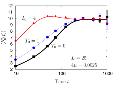
Figure 4: (Color online) Monte Carlo simulation (symbols) vs. numerical evaluation of Eq. (18) of the main text (lines). Simulations involve average over $10^{5}$ histories. Each history starts from an initial configuration drawn from the equilibrium ensemble at temperature $T_{0}$. The history contributes to the MSD if it is not absorbed up to time $t$.

IV D. Details of Monte-Carlo simulations for the case of harmonic absorption

Here, we give the details of the Monte Carlo (MC) simulations for the dynamics of the interface of length $L$ with tagged monomer at $0$ subject to absorption. We start the evolution from the initial $h^{0}$. For the equilibrated case, $h_{0}$ is just a Brownian bridge implemented as follows (note that in the program, we have set $h^{0}_{0}=h^{0}_{L-1}=0$ corresponding to $L-1$ independent monomers):

$$\widetilde{h}_{i} =\widetilde{h}_{i-1}+\sqrt{T_{0}}\,\xi_{i},$$

$$h_{i}^{0} =\widetilde{h}_{i}-\frac{i}{L-1}\widetilde{h}_{L-1}.$$ (55)

Here, $\xi_{i}$ is a Gaussian distributed random number with zero mean and unit variance, and $T_{0}$ is the initial temperature. The covariance matrix is therefore $\sigma_{ij}=T_{0}\big{[}\mathrm{min}(i,j)-ij/(L-1)\big{]}$.

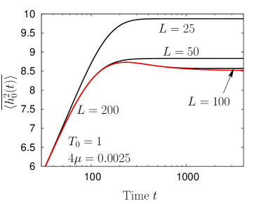
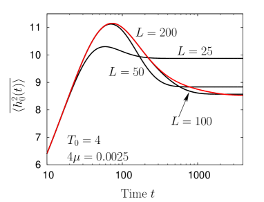
Figure 5: (Color online) Finite-size effects at two temperatures, $T_{0}=1,4$: Tagged MSD for different matrix size $L$. The convergence is observed for $L=200$.

Starting from $h^{0}$, the interface configuration is updated between times $t$ and $t+\delta t$ according to:

$$h_{i}(t+\delta t) = h_{i}(t)+\delta t\left[h_{i+1}(t)+h_{i-1}(t)-2h_{i}(t)\right]$$ (56)

$$+\sqrt{2\delta t}\,\eta_{i}(t),$$

for $i=1,2,\ldots,L-1$., while $\delta t\ll 1$ is a pre-assigned number. Following the update (56), the tagged monomer gets absorbed with probability $1-\exp(-\mu h_{0}^{2}\delta t)$. In case the tagged monomer is actually absorbed, the whole process of evolving the interface starts all over again. Figure 4 shows MC simulation results for the variance of the tagged particle displacement, compared with numerical evaluation of the matrix defined by Eq. (17) of the main text; we observe a very good agreement between the two.

Using Eq. (18) of the main text, we can study the limit of long polymers. By varying $L$, we show in Fig. 5 finite-size effects in the behavior of the variance of the tagged particle displacement for two different initial temperatures. In both cases. one observes a convergence in behavior for $L=200$.

References

• (1) P. G. de Gennes, Reptation of polymer chain in the presence of fixed obstacles, J. Chem. Phys. 55, 572 (1971).
• (2) J. Krug, H. Kallabis, S. N. Majumdar, S. J. Cornell, A. J. Bray and C. Sire, Persistence exponent for fluctuating interfaces, Phys. Rev. E 56, 2702 (1997).
• (3) D. Panja, Probabilistic phase space trajectory description for anomalous polymer dynamics, J. Phys.: Condens. Matter 23, 105103 (2011).
• (4) A. Taloni, A. Chechkin and J. Klafter, Generalized elastic model yields a fractional Langevin equation description, Phys. Rev. Lett. 104, 160602 (2010).s
• (5) B. B. Mandelbrot and J. W. van Ness, SIAM Rev. 10, 422 (1968).
• (6) A. N. Kolmogorov, Compus Rendus (Doklady) de l’Académie des sciences de l’URSS (N.S) 26, 115 (1940).
• (7) J.-C. Walter, A. Ferrantini, E. Carlon and C. Vanderzande, Fractional Brownian motion and the critical dynamics of zipping polymers, Phys. Rev. E 85, 031120 (2012).
• (8) Y. Kantor and M. Kardar, Anomalous Diffusion with Absorbing Boundary, Phys. Rev. E 69, 021806 (2004).
• (9) A. Zoia, A. Rosso and S. N. Majumdar, Asymptotic Behavior of Self-Affine Processes in Semi-Infinite Domains, Phys. Rev. Lett. 102, 120602 (2009).
• (10) D. Panja and G. T. Barkema, Simulations of two-dimensional unbiased polymer translocation using the bond fluctuation model, J. Chem. Phys. 132, 014902 (2010).
• (11) D. Panja, G. T. Barkema and R. C. Ball, Anomalous dynamics of unbiased polymer translocation through a narrow pore, J. Phys.: Condens. Matter 19, 432202 (2007).
• (12) J. Szymanski and M. Weiss, Elucidating the Origin of Anomalous Diffusion in Crowded Fluids, Phys. Rev. Lett. 103, 038102 (2009).
• (13) S. C. Weber, A. J. Spakowitz and J. A. Theriot, Bacterial Chromosomal Loci Move Subdiffusively through a Viscoelastic Cytoplasm, Phys. Rev. Lett. 104, 238102 (2010).
• (14) J.-H. Jeon, H. Monne, M. Javanainen and R. Metzler, Anomalous Diffusion of Phospholipids and Cholesterols in a Lipid Bilayer and its Origins, Phys. Rev. Lett. 109, 188103 (2012).
• (15) L. Lizana, T. Ambjörnsson, A. Taloni, E. Barkai and M. A. Lomholt, Foundation of fractional Langevin equation: Harmonization of a many-body problem, Phys. Rev. E 81, 051118 (2010).
• (16) E. Bertseva, D. Grebenkov, P. Schmidhauser, S. Gribkova, S. Jeney and L. Forró, Optical trapping microrheology in cultured human cells, Eur. Phys. J. E 35, 63 (2012).
• (17) T. Guérin, O. Bénichou and R. Voituriez, Non Markovian polymer reaction kinetics, Nature Chem. 4, 568 (2012).
• (18) T. Guérin, O. Bénichou and R. Voituriez, Reactive conformations and non-Markovian reaction kinetics of a Rouse polymer searching for a target in confinement, Phys. Rev. E 87, 032601 (2013).
• (19) T. Dieker, ”Simulation of fractional Brownian motion”, Master Thesis, http://www2.isye.gatech.edu/ adieker3.
• (20) A. K. Hartmann, S. N. Majumdar and A. Rosso, Sampling fractional Brownian motion in presence of absorption: A Markov chain method, Phys. Rev. E 88, 022119 (2013).
• (21) J.-H. Jeon and R. Metzler, Fractional Brownian motion and motion governed by the fractional Langevin equation in confined geometries, Phys. Rev. E 81, 021103 (2010).
• (22) P. Allegrini, M. Buiatti, P. Grigolini and B. J. West, Fractional Brownian motion as a nonstationary process: An alternative paradigm for DNA sequences, Phys. Rev. E 57, 4558 (1998).
• (23) D. Panja, Anomalous polymer dynamics is non-Markovian: memory effects and the generalized Langevin equation formulation, J. Stat. Mech. P06011 (2010).
• (24) A. D. Viñales and M. A. Despósito, Anomalous diffusion: Exact solution of the generalized Langevin equation for harmonically bounded particle, Phys. Rev. E 73, 016111 (2006).
• (25) M. A. Despósito and A. D. Viñales, Subdiffusive behavior in a trapping potential: Mean square displacement and velocity autocorrelation function, Phys. Rev. E 80, 021111 (2009).
• (26) D. S. Grebenkov, Time-averaged quadratic functionals of a Gaussian process, Phys. Rev. E 83, 061117 (2011).
• (27) S. F. Edwards and D. R. Wilkinson, The Surface Statistics of a Granular Aggregate, Proc. R. Soc. London Ser. A 381, 17 (1982).
• (28) H. Risken, The Fokker-Planck Equation: Methods of Solution and Applications, Springer, Berlin (1989).
• (29) C. W. Gardiner, Handbook of stochastic methods for physics, chemistry and the natural sciences, Springer (1989).
• (30) S. Redner, A Guide to First-Passage Processes, Cambridge University Press, New York, (2001).
• (31) A. J. Bray, S. N. Majumdar and G. Schehr, Persistence and first-passage properties in nonequilibrium systems, Adv. Phys. 62, 225 (2013).
• (32) R. Keesman, G. T. Barkema and D. Panja, Dynamical Eigenmodes of a Polymerized Membrane, J. Stat. Mech. P04009 (2013).
• (33) A. Zoia, A. Rosso and M. Kardar, Fractional Laplacian in bounded domains, Phys. Rev. E 76, 021116 (2007).
• (34) S. Gupta, S. N. Majumdar, C. Godrèche and M. Barma, Tagged particle correlations in the asymmetric simple exclusion process: Finite-size effects, Phys. Rev. E 76, 021112 (2007).
• (35) In one dimension, the difference between the Rouse chain and the EW interface is that the displacements are longitudinal in the former and transversal in the latter. For graphical reasons, we prefer to draw the interface.

References

• (1) H. Risken, The Fokker-Planck Equation: Methods of Solutions and Applications, Springer, Berlin (1989).
• (2) R. P. Feynman and A. R. Hibbs, Quantum Mechanics and Path Integrals, McGraw-Hill, New York (1965).
• (3) J. Krug, H. Kallabis, S. N. Majumdar, S. J. Cornell, A. J. Bray and C. Sire, Persistence exponent for fluctuating interfaces, Phys. Rev. E 56, 2702 (1997).
• (4) S. G. Samko, A. A. Kilbas, and O. I. Maritchev, Fractional Integral and Derivatives, Gordon and Breach, New York, 1993.
• (5) I. Podlubny, Fractional Differential Equations, Academic Press, London, 1999.
• (6) I. S. Gradshteyn and I. M. Ryzhik, Table of integrals, series and products, Academic Press, fifth edition (1994).
• (7) C. Texier, Mécanique quantique, Dunod, Paris (2011).