Three-dimensional MHD modeling of propagating disturbances in fan-like coronal loops

Abstract

Quasi-periodic propagating intensity disturbances (PDs) have been observed in large coronal loops in EUV images over a decade, and are widely accepted to be slow magnetosonic waves. However, spectroscopic observations from Hinode/EIS revealed their association with persistent coronal upflows, making this interpretation debatable. Motivated by the scenario that the coronal upflows could be cumulative result of numerous individual flow pulses generated by sporadic heating events (nanoflares) at the loop base, we construct a velocity driver with repetitive tiny pulses, whose energy frequency distribution follows the flare power-law scaling. We then perform 3D MHD modeling of an idealized bipolar active region by applying this broadband velocity driver at the footpoints of large coronal loops which appear open in the computational domain. Our model successfully reproduces the PDs with similar features as the observed, and shows that any upflow pulses inevitably excite slow magnetosonic wave disturbances propagating along the loop. We find that the generated PDs are dominated by the wave signature as their propagation speeds are consistent with the wave speed in the presence of flows, and the injected flows rapidly decelerate with height. Our simulation results suggest that the observed PDs and associated persistent upflows may be produced by small-scale impulsive heating events (nanoflares) at the loop base, and that the flows and waves may both contribute to the PDs at lower heights.

1. Introduction

Quasi-periodic propagating disturbances (PDs) have been found in large coronal loops (e.g. Nightingale et al., 1999; Berghmans & Clette, 1999) since the launch of SOHO and TRACE. The PDs usually propagate at a speed on the order of 100 km s^-1 which is close to the sound speed in the warm ($\sim$1 MK) corona, leading to their interpretation as slow magnetosonic waves (see, Ofman et al., 1999; Nakariakov et al., 2000, and a review by De Moortel, 2009). Under this assumption, the observed amplitude decay was explained in terms of compressive viscosity (Ofman et al., 2000) or thermal conduction (Nakariakov et al., 2000; De Moortel & Hood, 2004), and the quasi-periodic nature of these waves has been attributed to the leakage of $p$-modes (De Pontieu et al., 2005).

Alternatively, the PDs were also interpreted as recurring flows (or jets) because of their association with high-speed upflows in footpoint regions of AR loops found by Hinode/EIS (e.g. Sakao et al., 2007; Harra et al., 2008; Ugarte-Urra et al., 2011). Recent finding that quasi-periodic variations in intensity, Doppler velocity, line width, and line asymmetry are correlated in the upflow regions supported this interpretation (De Pontieu & McIntosh, 2010; Tian et al., 2011a, b).

Recently, using the 3D MHD model, Ofman et al. (2012) studied the excitation and propagation of slow magnetosonic waves in hot ($\sim$6 MK) closed loops driven by steady or periodic upflows. Here we expand their model to simulate the PDs in large warm loops using a broadband flow driver in order to understand the physics of the observed PDs.

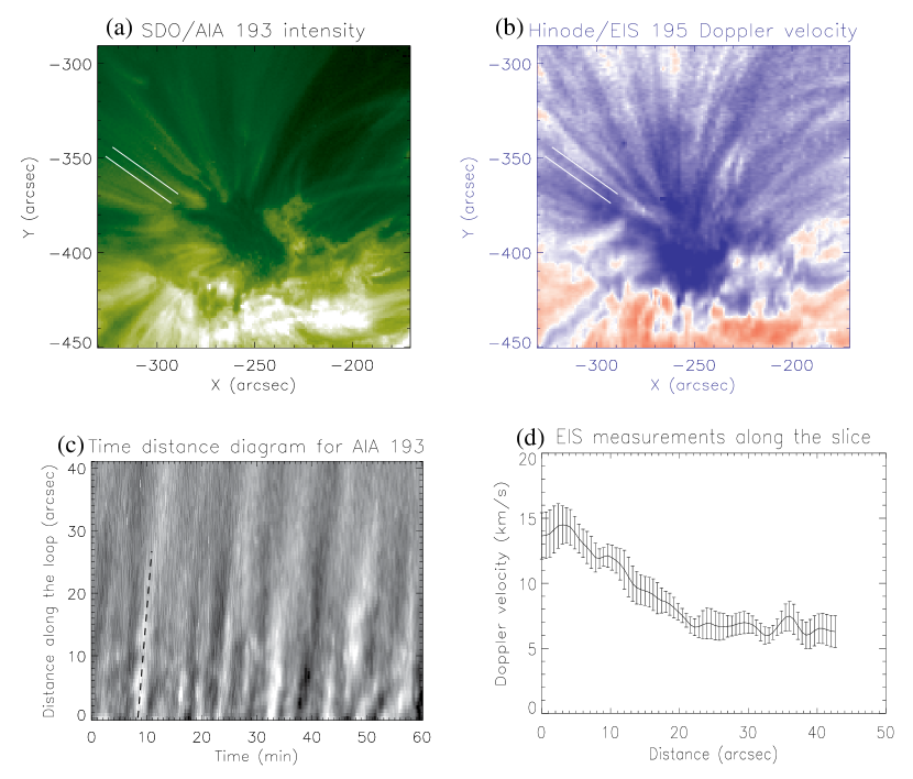
Figure 1.— Observations of propagating intensity disturbances and outflows on 2010 September 16 in AR 11106. (a) The image of SDO/AIA 193 Å at 11:57 UT. (b) The Doppler shift map of Hinode/EIS Fe xii 195.12 Å scanned from 10:38 to 11:57 UT. (c) A time-distance diagram of AIA 193 Å detrended intensity for a cut (shown with two parallel lines in (a)), averaged over a width of 11 pixels. The inclined dashed line indicates one propagating disturbance with a traveling speed of about 128 km s^-1. (d) The Doppler velocity profile of EIS Fe xii along the cut (shown in (b)).

2. Observational motivation

There has been plenty of evidence supporting that the PDs in coronal loops above sunspots are propagating slow magnetosonic waves. For example, the oscillations there have a period of about 3 minutes, same as the well-known umbral oscillations (De Moortel et al., 2002). The multi-wavelength observations indicate that the waves propagate from the photosphere through the chromosphere and transition region into the corona (e.g. Brynildse et al., 2002; Marsh et al., 2003; Jess et al., 2012). The propagation speeds of PDs are temperature dependent (Kiddie et al., 2012; Uritsky et al., 2013). The PDs propagate outward (e.g. in AIA 171) in the circular or arc shape, similar to those observed in the chromosphere (Liang et al., 2011, 2012). In contrast, the PDs in non-sunspot coronal loops appear to be different in some features. Their periods cover a wide range of about 3$-$30 min (De Moortel et al., 2002; Berghmans & Clette, 1999; Marsh et al., 2009; Wang et al., 2009; Krishna Prasad et al., 2012). The origin of those oscillations with longer ($\gtrsim$10 min) periods is hardly explained by the leakage of global $p$-modes (De Pontieu et al., 2005). In addition, they are usually associated with distinct upflows (e.g. Tian et al., 2011b), and the coherent scale of oscillations is relatively small (on the order of a few Mm) (McEwan & De Moortel, 2006; Kiddie et al., 2012). These differences suggest that the PDs in non-sunspot loops may have a different driver from the PDs in sunspot loops. One possible source could be recurrent small-scale impulsive events (nanoflares) at the coronal base (Ofman et al., 2012; Testa et al., 2013).

Figure 1 demonstrates a typical AR with upflows. The time-distance diagram shows the PDs propagating at almost constant speed of about 130 km s^-1 for a cut along fan-like loops in SDO/AIA 193 Å (Figures 1(a) and (c)). The Doppler velocity, measured by single Gaussian fits to the EIS Fe xii 195.12 Å line, shows a decrease from 15 km s^-1 to 6 km s^-1 along the same cut (Figures 1(b) and (d)). The purpose of our modeling is to understand the origin of PDs and their physical nature (flows or wave signatures).

3. Numerical model

Here, we briefly describe the 3D MHD numerical model used in this study (see, Ofman et al., 2012, for details). The resistive 3D MHD equations are solved with gravity and isothermal energy equation on a Cartesian $258^{3}$ grid using the modified Lax-Wendroff method with fourth-order stabilization term (e.g., Ofman & Thompson, 2002). The initial magnetic field is a dipole. To model an open-like loop with high spatial resolution, only the half domain of the dipole is chosen for the 3D computation (Figure 2), which is set as (0, 7) $\times$ ($-$3.5, 3.5) $\times$ (0, 3.5) in normalized distance units. The dipolar field is created by setting two unit magnetic charges of the opposite polarities at the positions ($\pm$1, 0, $-$2). The initial background density is given by the gravitationally stratified hydrostatic density

$$\rho=\rho_{0}{\,\rm exp}\left(\frac{1/(10+z)-1/10}{H}\right),$$ (1)

where $H=0.2k_{B}T_{0}R_{s}/(GM_{s}m_{p})$ is the normalized gravitational scale height, $R_{s}$ is the solar radius, $k_{B}$ is Boltzmann’s constant, $T_{0}$ is the temperature, $G$ is the universal gravitational constant, $M_{s}$ is the solar mass, and $m_{p}$ is the proton mass. The chosen and resulting normalization parameters are listed in Table 1. Van Doorsselaere et al. (2011) determined $\gamma$ (the adiabatic index) in loops and found that values are very close to unity expected in nearly isothermal plasma.

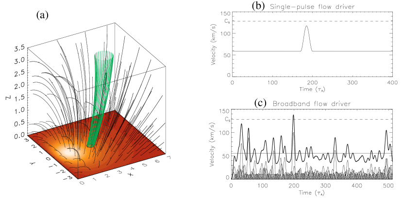
Figure 2.— (a) Initial magnetic field used for the model AR, which is taken as the half domain of a dipolar field. The intensity scale shows the longitudinal field component magnitude at the base of the AR, and the black lines show magnetic field lines. The green lines show a magnetic loop rooting on a flow region at the bottom boundary. (b) Time profile of velocity for a single pulse flow driver. (c) A broadband upflow driver, which consists of 205 random pulses with kinetic energies following a powerlaw frequency distribution of the index $\alpha$=2. The horizontal solid line indicates the resulting background level calculated by averaging the velocity over time.

A localized impulsive flow injection along the magnetic field is introduced at the lower boundary of the model AR as

$${\bf V}=V_{0}(x,y,z=0,t){\bf B}/|B|,$$ (2)

where

$$V_{0}(x,y,z=0,t)=V_{A0}A_{v}(t){\,\rm exp}\left[-\left(\frac{r}{w_{0}}\right)^{4}\right],$$ (3)

with $r=[(x-x_{0})^{2}+(y-y_{0})^{2}]^{1/2}$. The upflow is modeled with sharper-than-Gaussian cross-sectional profile, and imposed at the lower boundary in a region with $r\leq 2w_{0}$. The parameters are $x_{0}$ = 3.0, $y_{0}$ = 0, and $w_{0}$ = 0.12. We study two cases of upflow velocity: (1) a single pulse with constant background; (2) multiple pulses with broadband frequency distribution of energy. In the first case, we take $A_{v}(t)$ in the form,

$$A_{v}(t)=\left\{\begin{array}[]{ll}A_{0}&\quad(0<t<t_{1}\quad{\rm or}\quad t_{2}<t<t_{max})\\ A_{0}+\frac{1}{2}A_{0}[1-{\rm cos}\frac{2\pi(t-t_{1})}{P}]&\quad(t_{1}\leq t\leq t_{2})\end{array}\right.,$$ (4)

where the parameters $P=t_{2}-t_{1}$=30, $t_{1}$=170, $t_{2}$=200, $t_{max}$=400, and $A_{0}$ = 0.01 are set, so that the velocity driver has the maximum amplitude of 0.02, which is subsonic (Figure 2(b)). In the second case, we construct a broadband driver with $N$ individual pulses of the same lifetime ($P$=15) and the same shape in the form

$$A_{i}(t)=\frac{1}{2}A_{i0}[1-{\rm cos}\frac{2\pi(t-t_{i})}{P}]\quad(t_{i}\leq t\leq t_{i}+P),~{}i=1,2,...,N$$ (5)

and assuming that they occur subsequently with a fixed rate ($\Delta{t}=t_{i+1}-t_{i}=P/6$). We further assume the kinetic energy of flow pulses (defined as $E_{i}=A_{i0}^{2}$) follows a powerlaw frequency distribution ($df/dE\propto E^{-\alpha}$). For AR soft X-ray flares and microflares, it has been observed that the frequency distribution of their energy content has the index of about 1.8 (e.g. Wang et al., 2006). Here we randomly generate $N$ pulses for a powerlaw distribution with $\alpha=2$ and the velocity amplitudes in the range 10 to 110 km s^-1. Figure 2(c) shows the constructed velocity profile that includes about 26 visible peaks and a background (with a mean of 55$\pm$18 km s^-1) over a time of 513 $\tau_{A}$. The remaining boundary conditions are same as used in Ofman et al. (2012).

In the low-$\beta$ condition of the nearly ideal coronal plasma, both the plasma motion and slow magnetosonic wave propagation are nearly along the magnetic field lines (i.e., the magnetic field is nearly unaffected by the flow). Thus we can determine whether the simulated PDs are the signature of flows or waves, by comparing their “observed” paths (traveling distances as a function of time) with those predicted. Given the time-distance distribution ($V(s,t)$) of velocities along a loop, we calculate the flow path by integrating the following quantity numerically,

$$s=\int_{t_{0}}^{t}V(s,t)dt,$$ (6)

and calculating the wave path by integrating

$$s=\int_{t_{0}}^{t}(V(s,t)+C_{t}(s))dt,$$ (7)

with the initial condition $s$=0 at $t=t_{0}$, where $C_{t}(s)=(C_{s}^{-2}+V_{A}(s)^{-2})^{-1/2}$ is the tube speed for a straight cylinder (Roberts et al., 1984).

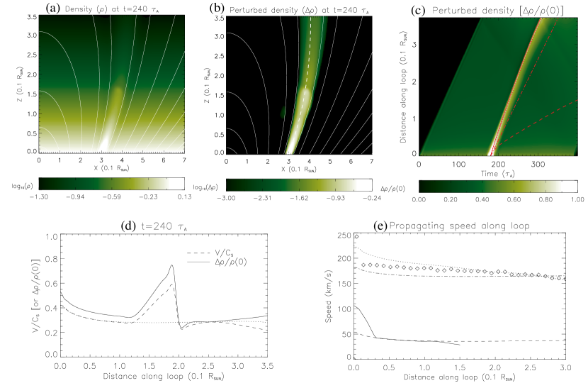
Figure 3.— The modeling with a single pulse flow driver. (a) The density in the $xz$-plane at the center of the AR at t=240 $\tau_{A}$, and (b) Same as (a) but for the perturbed density. The overlaid white lines are magnetic field lines in this plane. (c) Time-distance diagram of the perturbed density for a cut along the loop (dashed line in (b)). The solid and dashed lines are the predicted paths for the wave front and the flow, respectively. The dotted line indicates the peak positions of the density disturbance measured with the Gaussian fit. The dot-dashed line has a slope equal to the sound speed ($C_{s}$). (d) Spatial profiles of velocity (dashed line) and perturbed density (solid line) along the loop at t=240 $\tau_{A}$. The pre-pulse velocity profile (at t=159 $\tau_{A}$) is overplotted with the dotted line. (e) Spatial profiles of the wave propagation speed derived from the theoretical prediction (dotted line) and from the measured path of density disturbance (Diamonds). The dashed line represents the velocity for background flow ($V_{bg}(s)$, taken at t=159 $\tau_{A}$). The dot-dashed line indicates the wave speed estimated with $C_{s}+V_{bg}(s)$. The solid line indicates the velocity variation along the flow path.

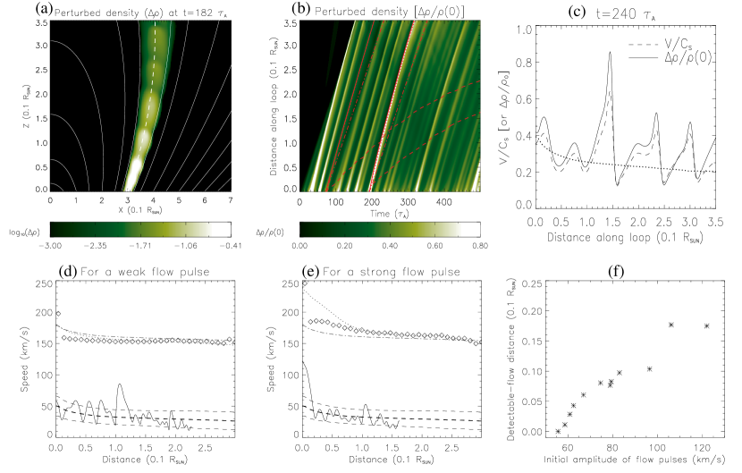
Figure 4.— Similar as Figure 3 but for a broadband upflow driver. The dotted line in (c) indicates the spatial profile of velocity averaged over time. The annotations for (d) and (e) are same as Figure 3(e) but for the two flow pulses analyzed in (b). The dashed lines are the time-averaged velocity (for background flow) and the standard deviations. (f) The detectable distance of flow pulses as a function of the initial amplitude (see text for detail).

4. Numerical results

First, we report the results in the single pulse case, where an upflow pulse could be produced by a small flare. Figures 3(a) and (b) show the snapshots of density and its perturbation in the xz-plane at $t=240\tau_{A}$. The steady inflow first forms a steady fan-like loop, and then the upflow pulse leads to a density disturbance traveling along the loop. Figure 3(d) shows the spatial profiles of velocity and perturbed density ($(\rho(s,t)-\rho(s,0))/\rho(s,0)$) at $t=240\tau_{A}$, indicating an in-phase relationship between them and a deceleration of background flow at lower heights. We calculated the flow and wave paths for this pulse in the time-distance diagram (Figure 3(c)). Obviously, the wave path (solid line) coincides well with that of the propagating density disturbance (PD, dotted line), which is measured by the Gaussian fits to the time profiles at each height. In Figure 3(e), we compared the measured speeds of the PD (Diamonds, by taking the derivatives of the time profile of peak positions) with the wave speeds theoretically predicted ($V(s,t)+C_{t}(s)$, dotted line) and the velocity of injected flow pulse (solid line). We also calculated another estimate of the wave speed using $C_{s}+V_{bg}(s)$ (dot-dashed line), where $V_{bg}(s)$ is the velocity for background flow. We find that the variation of the measured PD speeds agrees well with the theoretically expected phase speed in the presence of background flow, while the velocity of injected flow pulse is much smaller and shows a drastic drop to the background level. This indicates that the PD generated in the simulation is dominated by the wave signature, whereas the contribution of injected high-speed flows is only present at lower heights.

We now present the results of the broadband flow case, where quasi-periodic pulses are assumed to be produced by recurrent nanoflares. Figures 4(a) show the propagation of quasi-periodic density disturbances in the xz-plane at $t=182\tau_{A}$. Figure 4(c) compares the density perturbation and velocity profiles along the loop at $t=240\tau_{A}$, showing that their variations are roughly in phase, consistent with the features of propagating slow magnetosonic waves. The background flow along the loop was calculated by averaging the velocity over time at each height, showing a decrease with height. For a comparison we calculated the wave and flow paths for the two flow pulses, a weak one (at $t=75\tau_{A}$) with the amplitude close to that of background flow and a strong one (at $t=195\tau_{A}$) with the amplitude close to the sound speed. Figure 4(b) shows that for either weak or strong flow pulse, the wave path coincides well with the PD. For the weak pulse the flow is immediately separated from the PD after injection, suggesting that the PD is mainly the wave signature, whereas for the strong pulse the flow is visible within the PD over a distance of about $D_{flow}$=0.22, where $D_{flow}$ (named the detectable-flow distance) is defined as the distance over which the peak velocity of pulse remains at least 15% above the background flow. Figure 4(f) shows that $D_{flow}$ is proportional to the initial amplitudes of pulses. Figure 4(e) shows that the propagation speed of the PD generated by this strong pulse agrees well the predicted wave speed except at the lower heights, where we notice that the speeds of PD are better consistent with the wave speeds estimated by $C_{s}+V_{bg}(s)$. This may be because the flows highly deviate from the (quasi-) steady state at lower heights, as indicated by a quick deceleration. This suggests that the PDs are dominated by the wave signature with the flow contribution only at lower heights. For the 12 generated PDs, we measured their average propagating speeds over a distance of $s=1$ by the linear fitting to their propagation paths, and obtained the mean value of 165$\pm$9 km s^-1. In comparison, we also measured the average speeds of their injected flows using the same method, and obtained the mean of 37$\pm$5 km s^-1. Thus, the density disturbances produced by the upflow pulses propagate at a speed on average about four times faster than the corresponding injected flows.

It should be pointed out that the PDs can be modeled in 1D in certain simplified restrictive cases. However, as we find from several 1D test calculations, the results may differ significantly from the 3D MHD model with more realistic divergent and curved magnetic geometry, and with non-uniform injected flow profile. We have also made two additional runs for a flux tube with larger and smaller divergences respectively, by adjusting the depth of the dipole source, and found similar results in all cases, i.e., the waves dominate PDs from very low height. In the case of smaller divergence the height of detectable flow is somewhat higher than in the case of larger divergence.

Table 1List of physical parameters used in the model.

Quantities	Single pulse case	Broad band case
Parameters for flow driver
Background flow (km s-1)	59	55 $\pm$ 18
Pulse amplitude (km s-1)	59	10 $-$ 110
Pulse period (min)	6	3
Measured quantitie
Wave speed (km s-1)	184	165 $\pm$ 9
Flow speed (km s-1)	41	37 $\pm$ 5
Model nomalization parameters
Length scale ($a$)		0.1 Rs
Magnetic field ($B_{0}$)		100 G
Temperature ($T_{0}$)		1 MK
Number density ($n_{0}$)		1.38$\times{10}^{9}$ cm-3
Alfvén speed ($V_{A0}$)		5872 km s-1
Alfvén time ($\tau_{A}$)		12 s
Sound speed ($C_{s}$)		128 km s-1
Gravitational scale height ($H_{0}$)		60 Mm

5. Discussion and conclusions

To determine whether propagating intensity disturbances seen in EUV imaging observations of coronal loops are flows or waves, we develop a 3D MHD model with the geometry and initial state in qualitative agreement with typical observations. We first use the driver of a single upflow pulse with steady background at the footpoints of open-like magnetic fields (i.e., a long loop initially in hydrostatic equilibrium that closes outside the computational domain) to study the effects of high-speed jets in the persistent upflow region observed by Hinode/EIS (e.g. Ugarte-Urra et al., 2011; Nishizuka & Hara, 2011). The simulations show that the injection of a velocity pulse (with the parameters typically for observations) inevitably excites a slow magnetosonic wave disturbance propagating along the loop at the phase speed of about the sound speed plus the background flow velocity. This result suggests that the observed quasi-periodic PDs, when interpreted as slow magnetosonic waves, are not necessarily excited by a quasi-periodic driver such as the photospheric $p$-mode leakage, but can be produced by recurrent small-scale impulsive energy release such as nanoflares (Hara et al., 2008; Ofman et al., 2012), or reconnection jets (e.g. Yokoyama & Shibata, 1995; Gontikakis et al., 2009). Following this idea, we construct a broadband flow driver with repetitive tiny pulses, and successfully reproduce the quasi-periodic PDs which are qualitatively consistent with the observations. We find whether upflow pulses are small (with amplitudes close to the persistent background flow of the order of 20$-$30 of km s^-1), or strong (with amplitudes of the order of the sound speed), the generated PDs in our simulations are dominated by the wave signature as their propagation speeds are consistent with the wave speed in the presence of flows; for the latter case the injected flows may be detectable at heights up to $\sim$20 Mm, comparable to the detection lengths of observed PDs (McEwan & De Moortel, 2006), but these flows decelerate rapidly with height primarily due to gravity and the downward thermal pressure gradient that results from the relative density increase due to the initial upflow material.

Our simulations help solve several controversies: the results suggest that persistent upflows observed with Hinode/EIS (see Figure 1(b)) may be a collective effect of unresolved tiny velocity pulses produced by nanoflares at the coronal base, while the individual quasi-periodic PDs imaged with TRACE or SDO/AIA (see Figure 1(c)) correspond to low frequency larger events. This scenario can eliminates the difficulty explaining the origin of longer-period (10$-$30 minutes) oscillations (or harmonics) of PDs by the leakage of global $p$-modes. Note that it is possible that the nanoflare-produced broadband flows are modulated by the 5-minutes $p$-mode oscillations in non-sunspot loops (McEwan & De Moortel, 2006). In addition, if the broadband periodicity of PDs is the effect of nanoflares, they may be used to diagnose the energy distribution of nanoflares.

Our results also suggest a possible connection between the wave and flow interpretations for PDs. On the one hand, spectroscopic features such as line blue asymmetries and width broadening infer the presence of high-speed ($\sim$ 100 km s^-1) outflows (De Pontieu & McIntosh, 2010; Tian et al., 2011a). On the other hand, our MHD modeling indicates that any subsonic flow pulses injected at the loop footpoints will inevitably excite slow magnetosonic wave disturbances propagating ahead of the injected flows. Thus, the flows and waves may both contribute to the formatin of PDs. Observations show that the PDs sometimes can reach higher altitudes (on the order of the gravitational scale height) at almost constant speed (Wang et al., 2009; Marsh et al., 2009; Krishna Prasad et al., 2012). This feature is consistent with our simulation results and suggests the dominant contribution of waves, while high-speed dynamic flows may be only present at lower heights. EIS observations show that the line blue asymmetries are detectable mainly within a distance of about 20 Mm above loop’s footpoints (Nishizuka & Hara, 2011; Tian et al., 2011b; McIntosh et al., 2012). A future work that compares synthetic line profiles in the PDs with observations will help test the model and confirm the above scenario.

Although our model is limited to the idealization of an isothermal plasma, it can still model the flows produced by impulsive heating. Because the impulsive heating increases the thermal pressure to drive the flow along the magnetic field, it does not matter whether the pressure pulse is produced by a pulse of density, temperature, or both. In addition, to obtained flow pulses (rather than waves) at nearly constant sonic or supersonic speeds as observed for the PDs at higher heights, some non-thermal effects such as magnetic slingshot effect due to magnetic reconnection (e.g. Gontikakis et al., 2009), or non-isothermal effects such as the temperature of outflows increasing with height (Imada et al., 2011) may be required. However, no evidence for these effects have been found in imaging or spectral observations of PDs so far. This also justifies the use of the isothermal energy equation in our model. Although the model shows qualitatively that PD signatures are dominated by slow magnetosonic waves from low heights using idealized active region model, in real coronal loops the quantitative sensitivity of these signatures to the details of the field configuration needs to be studied, and any direct comparison of the observed signatures to the modeled signatures has to include a proper model of the corresponding particular solar magnetic fields.

References

- Berghmans & Clette (1999) Berghmans, D. & Clette, F. 1999, Sol. Phys., 186, 207
- Bryans et al. (2010) Bryans, P., Young, P. R., & Doschek, G. A. 2010, ApJ, 715, 1012
- Brynildse et al. (2002) Brynildsen, N., Maltby, P., Fredvik, T., & Kjeldseth-Moe, O. 2002, Sol. Phys., 207, 259
- De Moortel et al. (2002) De Moortel, I., Ireland, J., Hood, A. W., & Walsh, R. W. 2002, A&A, 387, L13
- De Moortel & Hood (2004) De Moortel, I., & Hood, A. W. 2004, A&A, 415, 705
- De Moortel (2009) De Moortel, I. 2009, Space Sci. Rev., 149, 65
- De Pontieu et al. (2005) De Pontieu, B., Erdélyi, R., De Moortel, I. 2005, ApJ, 624, L61
- De Pontieu & McIntosh (2010) De Pontieu, B., & McIntosh, S. W. 2010, ApJ, 722, 1013
- Gontikakis et al. (2009) Gontikakis, C., Archontis, V., & Tsinganos, K. 2009, A&A, 506, L45
- Hara et al. (2008) Hara, H., Watanabe, T., Harra, L. K., et al. 2008, ApJ, 678, L67
- Harra et al. (2008) Harra, L. K., Sakao, T., Mandrini, C. H., et al. 2008, ApJ, 676, L147
- Imada et al. (2011) Imada, S., Hara, H., Watanabe, T., et al., ApJ, 743, 57
- Jess et al. (2012) Jess, D. B., De Moortel, I., Mathioudakis, M., et al. 2012, ApJ, 757, 160
- Kiddie et al. (2012) Kiddie, G., De Moortel, I., Del Zanna, G., et al. 2012, Sol. Phys., 279, 427
- Krishna Prasad et al. (2012) Krishna Prasad, S., Banerjee, D. & , Van Doorsselaere, T. & Singh, J. 2012, A&A546, 50
- Liang et al. (2011) Liang, H. F., Ma, L., Yang, R., et al. 2011, PASJ, 63, 575
- Liang et al. (2012) Liang, H. F., Yang, W. G., Ma, L.,& Yang, R. J. 2012, New Astron., 17, 112
- Marsh et al. (2003) Marsh, M. S., Walsh, R. W., De Moortel, I., & Ireland, J. 2003, A&A, 404, L37
- Marsh et al. (2009) Marsh, M. S., Walsh, R. W., & Plunkett, S. 2009, ApJ, 697, 1674
- McEwan & De Moortel (2006) McEwan, M. P., & De Moortel, I. 2006, 448, 763
- McIntosh et al. (2012) McIntosh, S. W., Tian, H., Sechler, M., & De Pontieu, B. 2012, ApJ, 749, 60
- Nakariakov et al. (2000) Nakariakov, V. M., Verwichte, E., Berghmans, D., & Robbrecht, E. 2000, A&A, 362, 1151
- Nightingale et al. (1999) Nightingale, R. W., Aschwanden, M. J., & Hurlburt, N. E. 1999,Sol. Phys., 190, 249
- Nishizuka & Hara (2011) Nishizuka, N., & Hara, H. 2011, ApJ, 737, L43
- Ofman et al. (1999) Ofman, L., Nakariakov, V. M., & Deforest, C. E. 1999, ApJ, 514, 441
- Ofman et al. (2000) Ofman, L., Nakariakov, V. M., & Sehgal, N. 2000, ApJ, 533, 1071
- Ofman & Thompson (2002) Ofman, L., & Thompson, B. J. 2002, ApJ, 574, 440
- Ofman et al. (2012) Ofman, L., Wang, T. J., & Davila, J. M. 2012, ApJ, 754,111
- Roberts et al. (1984) Roberts, B., Edwin, P. M., & Benz, A. O. 1984, ApJ, 279, 857
- Sakao et al. (2007) Sakao, T., Kano, R., Narukage, N., et al. 2007, Science, 318, 1585
- Testa et al. (2013) Testa, P., De Pontieu, B., Martinez-Sykora, J., et al. 2013, ApJ, 770, L1
- Tian et al. (2011a) Tian, H., McIntosh, S. W., & De Pontieu, B. 2011a, ApJ, 727, L37
- Tian et al. (2011b) Tian, H., McIntosh, S. W., De Pontieu, B., et al. 2011b, ApJ, 738, 18
- Ugarte-Urra et al. (2011) Ugarte-Urra, I., & Warren, H. P. 2011, ApJ, 730, 37
- Uritsky et al. (2013) Uritsky, V. M., Davila, J. M., Nicholeen, M. V., & Ofman, L. 2013, ApJ, submitted
- Van Doorsselaere et al. (2011) Van Doorsselaere, T., Wardle, N., Del Zanna, G., et al. 2011, ApJ, 727, L32
- Wang et al. (2006) Wang, T. J., Innes, D. E., & Solanki S. K. 2006, A&A, 455, 1105
- Wang et al. (2009) Wang, T. J., Ofman, L., Davila, J. M., & Mariska, J. T. 2009, A&A, 503, L25
- Yokoyama & Shibata (1995) Yokoyama,T. & Shibata, K. 1995, Nature, 375, 42