Colombeau Algebra: A pedagogical introduction

Abstract

A simple pedagogical introduction to the Colombeau algebra of generalised functions is presented, leading the standard definition.

1 Introduction

This is a pedagogical introduction to the Colombeau algebra of generalised functions. I will limit myself to the Colombeau Algebra over ${\mathbb{R}}$. Rather than ${\mathbb{R}}^{n}$. This is mainly for clarity. Once the general idea has been understood the extension to ${\mathbb{R}}^{n}$ is not too difficult. In addition I have limited the introduction to ${\mathbb{R}}$ valued generalised functions. To replace with ${\mathbb{C}}$ valued generalised functions is also rather trivial.

I hope that this guide is useful in your understanding of Colombeau Algebras. Please feel free to contact me.

There is much general literature on Colombeau Algebras but I found the books by Colombeau himself[1] and the Masters thesis by Tạ Ngọc Trí[2] useful.

2 Test functions and Distributions

The set of infinitely differentiable functions on ${\mathbb{R}}$ is given by

$${\cal F}({\mathbb{R}})={\left\{\phi:{\mathbb{R}}\to{\mathbb{R}}\ |\ \phi^{(n)}\text{ exists for all $n$}\right\}}$$ (1)

Test functions are those function which in addition to being smooth are zero outside an interval, i.e.

$${\cal F}_{0}({\mathbb{R}})={\left\{\phi\in{\cal F}({\mathbb{R}})\ |\ \text{there exists $a,b\in{\mathbb{R}}$ such that $f(x)=0$ for $x<a$ and $x>b$}\right\}}$$ (2)

I will assume the reader is familiar with distributions, either in the notation of integrals or as linear functionals. Thus the most important distributions is the Dirac-$\delta$. This is defined either as a “function” $\delta(x)$ such that

$${\int_{-\infty}^{\infty}}\delta(x)\phi(x)dx=\phi(0)$$ (3)

Or as a distribution $\Delta:{\cal F}_{0}({\mathbb{R}})\to{\mathbb{R}}$,

$$\Delta[\phi]=\phi(0)$$ (4)

We will refer to (3) as the integral notation and (4) as the Schwartz notation. An arbitrary distribution will be written either as $\psi(x)$ for the integral notation or $\Psi$ for the Schwartz notation.

3 Function valued distributions

The first step in understanding the Colombeau Algebra is to convert distributions into a new object which takes a test functions $\phi$ and gives a functions

$$\boldsymbol{A}:{\cal F}_{0}({\mathbb{R}})\to{\cal F}({\mathbb{R}})$$

This is achieved by using translation of the test functions. Given $\phi\in{\cal F}_{0}$ then let

$$\phi^{y}\in{\cal F}_{0}({\mathbb{R}})\,,\qquad\phi^{y}(x)=\phi(x-y)$$ (5)

Then in integral notation

$$\overline{\psi}[\phi](y)={\int_{-\infty}^{\infty}}\psi(x)\phi(x-y)dx$$ (6)

and in Schwartz notation

$$\overline{\Psi}[\phi](y)=\Psi[\phi^{y}]$$ (7)

We will define the Colombeau Algebra in such a way that they include the elements $\overline{\psi}$ and $\overline{\Psi}$. The overline will be used to covert distributions into elements of the Colombeau algebra.

We label the set of all function valued functionals

$${\cal H}({\mathbb{R}})={\left\{\boldsymbol{A}:{\cal F}_{0}({\mathbb{R}})\to{\cal F}({\mathbb{R}})\right\}}$$ (8)

We see below that we need to restrict ${\cal H}({\mathbb{R}})$ further in order to define the Colombeau algebra ${\cal G}({\mathbb{R}})$.

Observe that we use a slightly non standard notation. Here $\boldsymbol{A}[\phi]:{\mathbb{R}}\to{\mathbb{R}}$ is a function, so that given a point $x\in{\mathbb{R}}$ then $\boldsymbol{A}[\phi](x)\in{\mathbb{R}}$. One can equally write $\boldsymbol{A}[\phi](x)=\boldsymbol{A}(\phi,x)$, which is the standard notation in the literature. However I claim that the notation $\boldsymbol{A}[\phi](x)$ does have advantages.

4 Three special examples.

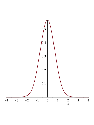
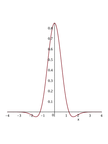
Figure 1: Plots of $\phi_{1}\in{\mathbb{A}}_{1}$ and $\phi_{3}\in{\mathbb{A}}_{3}$

For the Dirac-$\delta$ we see that

$$\overline{\delta}=\overline{\Delta}=\boldsymbol{R}$$ (9)

where $\boldsymbol{R}\in{\cal H}({\mathbb{R}})$ is the reflection map

$$\boldsymbol{R}[\phi](y)=\phi(-y)$$ (10)

This is because

$$\overline{\delta}[\phi](y)={\int_{-\infty}^{\infty}}\delta(x)\phi(x-y)dx=\phi(-y)$$

and is Schwartz notation

$$\overline{\Delta}[\phi](y)=\Delta[\phi^{y}]=\phi^{y}(0)=\phi(-y)$$

Regular distribution: Given any function $f\in{\cal F}$ then there is a distribution $f^{D}$ given by

$$f^{D}[\phi]={\int_{-\infty}^{\infty}}f(x)\phi(x)dx$$ (11)

Thus we set ${\overline{f}}=\overline{f^{D}}\in{\cal H}({\mathbb{R}})$ as

$${\overline{f}}[\phi](y) ={f^{D}}[\phi^{y}]={\int_{-\infty}^{\infty}}f(x)\phi(x-y)dx$$ (12)

The other important generalised functions are the regular functions. That is given $f\in{\cal F}$ we set

$$\tilde{f}\in{\cal H}({\mathbb{R}})\,,\qquad\tilde{f}[\phi]=f\quad\textup{that is}\quad\tilde{f}[\phi](y)=f(y)$$ (13)

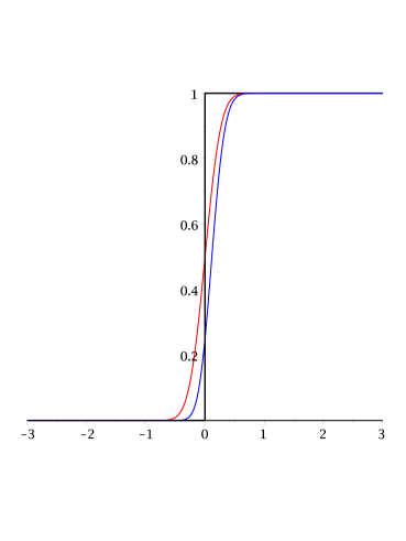
Figure 2: Heaviside (black) and $\overline{\theta}[\phi]$ (red) and $\big{(}\overline{\theta}[\phi]\big{)}^{2}$ (blue)

The effect of replacing $\overline{\psi}[\phi_{\epsilon}]$ is to smooth out $\psi$. Examples of $\phi$ are given in figure 1. The action $\overline{\theta}[\phi]$ where $\theta$ is the Heaviside function is given in figure 2.

5 Sums and Products

Given two Generalised functions $\boldsymbol{A},\boldsymbol{B}\in{\cal H}({\mathbb{R}})$ then we can define there sum and product in the natural way

$$\boldsymbol{A}+\boldsymbol{B}\in{\cal H}({\mathbb{R}})\quad\textup{via}\quad(\boldsymbol{A}+\boldsymbol{B})[\phi]=\boldsymbol{A}[\phi]+\boldsymbol{B}[\phi]\quad\textup{i.e.}\quad(\boldsymbol{A}+\boldsymbol{B})[\phi](y)=\boldsymbol{A}[\phi](y)+\boldsymbol{B}[\phi](y)$$ (14)

and

$$\boldsymbol{A}\boldsymbol{B}\in{\cal H}({\mathbb{R}})\quad\textup{via}\quad(\boldsymbol{A}\boldsymbol{B})[\phi]=\boldsymbol{A}[\phi]\boldsymbol{B}[\phi]\quad\textup{i.e.}\quad(\boldsymbol{A}\boldsymbol{B})[\phi](y)=\boldsymbol{A}[\phi](y)\boldsymbol{B}[\phi](y)$$ (15)

We see that the product of delta functions $\overline{\delta}{}^{2}\in{\cal H}({\mathbb{R}})$ is clearly defined. That is

$$\overline{\delta}{}^{2}[\phi](y)=(\overline{\delta}[\phi]\overline{\delta}[\phi])(y)=\overline{\delta}[\phi](y)\overline{\delta}[\phi](y)=\big{(}\phi(-y)\big{)}^{2}$$

Although this is a generalised function, it does not correspond to a distribution, via (7). That is there is no distribution $\Psi$ such that $\overline{\Psi}=(\overline{\delta})^{2}$.

Likewise we can see from figure 2 that $(\overline{\theta})^{2}[\phi]=\big{(}\overline{\theta}[\phi]\big{)}^{2}\neq\overline{\theta}[\phi]$.

6 Making ${\overline{f}}$ and ${\tilde{f}}$ equivalent

Now compare the generalised function ${\overline{f}}$ and ${\tilde{f}}$ (12),(13). We would like these two generalised functions to be equivalent, so that we can write ${\overline{f}}\sim{\tilde{f}}$. One of the results of making ${\overline{f}}\sim{\tilde{f}}$ is that if $f,g\in{\cal F}$ then

$$\overline{(fg)}\sim\widetilde{(fg)}=\widetilde{f}\ \widetilde{g}\sim\overline{f}\ \overline{g}$$

In the Colombeau algebra, which is a quotient of equivalent generalised functions, we say that ${\overline{f}}$ and ${\tilde{f}}$ are the same generalised function.

The goal therefore is to restrict the set of possible $\phi$ so that when they are acted upon by $({\overline{f}}-{\tilde{f}})$ the difference is small, where small will be made technically precise. When we think of quantities being small, we need a 1-parameter family of such quantities such that in the limit the difference vanishes. Here we label the parameter $\epsilon$ and we are interested in the limit $\epsilon\to 0$ from above, i.e. with $\epsilon>0$. Given a one parameter set of functions $g_{\epsilon}\in{\cal F}$ then one meaning to say $g_{\epsilon}$ is small is if $g_{\epsilon}(y)\to 0$ for all $y$. However we would like a whole hierarchy of smallness. That is for any $q\in{\mathbb{N}}_{0}={\mathbb{N}}\bigcup{\left\{0\right\}}$ then we can say

$$g_{\epsilon}={\cal O}(\epsilon^{q})$$ (16)

if $\epsilon^{-q}g_{\epsilon}(y)$ is bounded as $\epsilon\to 0$. Note that we use bounded, rather that tends to zero. However, clearly, if $g_{\epsilon}={\cal O}(\epsilon^{q})$ then $\epsilon^{-q+1}g_{\epsilon}\to 0$ as $\epsilon\to 0$.

We will also need the notion of $g_{\epsilon}={\cal O}(\epsilon^{q})$ where $q<0$. Thus we wish to consider functions which blow up as $\epsilon\to 0$, but not too quickly. Such functions will be called moderate.

Technically we say $g_{\epsilon}$ satisfies (16) if for any interval $(a,b)$ there exists $C>0$ and $\eta>0$ such that

$$\epsilon^{-q}|g_{\epsilon}(x)|<C\qquad\textup{for all}\qquad a\leq y\leq b\qquad\textup{and}\qquad 0<\epsilon<\eta$$ (17)

We introduce the parameter $\epsilon$ via the test functions, replacing $\phi\in{\cal F}_{0}$ with $\phi_{\epsilon}\in{\cal F}_{0}$ where

$$\phi_{\epsilon}(x)=\frac{1}{\epsilon}\phi\Big{(}\frac{x}{\epsilon}\Big{)}$$ (18)

Observe at as $\epsilon\to 0$ then $\phi_{\epsilon}$ becomes narrower and taller, in a definite sense more like a $\delta$-function. Thus we consider a generalised function $\boldsymbol{A}$ to be small, if for some appropriate set of test functions $\phi\in{\cal F}_{0}$ and for some $q\in{\mathbb{Z}}$, $\boldsymbol{A}[\phi_{\epsilon}]={\cal O}(\epsilon^{q})$.

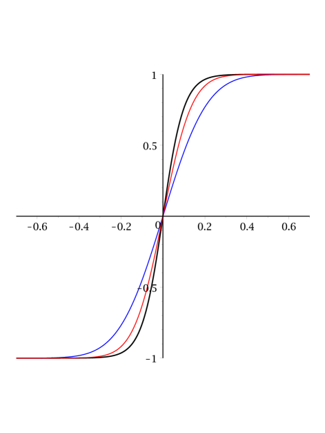
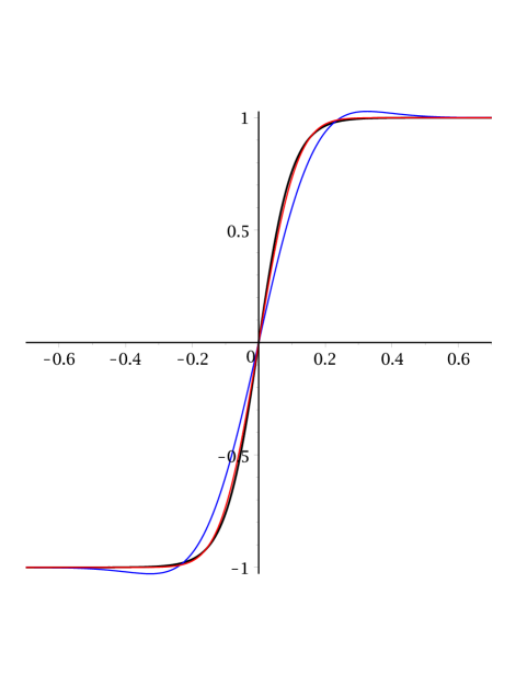
$f$ (back), ${\overline{f}}[\phi_{1}|_{\epsilon=0.2}]$ (blue) and ${\overline{f}}[\phi_{1}|_{\epsilon=0.1}]$ (red).	$f$ (back), ${\overline{f}}[\phi_{3}|_{\epsilon=0.2}]$ (blue) and ${\overline{f}}[\phi_{3}|_{\epsilon=0.1}]$ (red).
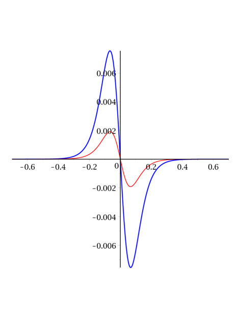
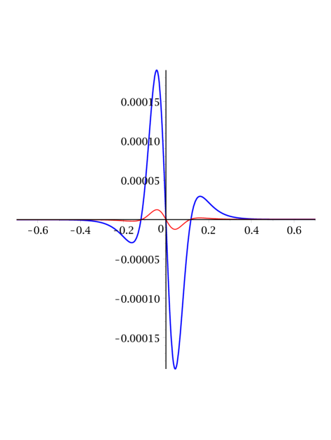
$({\overline{f}}-{\tilde{f}})[\phi_{1}|_{\epsilon=0.02}]$ (blue) and $({\overline{f}}-{\tilde{f}})[\phi_{1}|_{\epsilon=0.01}]$ (red).	$({\overline{f}}-{\tilde{f}})[\phi_{3}|_{\epsilon=0.02}]$ (blue) and $({\overline{f}}-{\tilde{f}})[\phi_{3}|_{\epsilon=0.01}]$ (red).

Figure 3: Plots of ${\overline{f}}[\phi_{\epsilon}]$ with $f(x)=\tanh(10x)$

Let us first restrict $\phi\in{\cal F}_{0}$ to be test function which integrate to $1$. That is we define ${\mathbb{A}}_{0}\subset{\cal F}_{0}$,

$${\mathbb{A}}_{0}={\left\{\phi\in{\cal F}_{0}\,\Big{|}\,{\int_{-\infty}^{\infty}}\phi(x)dx=1\right\}}$$ (19)

Given $\phi\in{\mathbb{A}}_{0}$ and setting $z=(x-y)/\epsilon$ so that $x=y+\epsilon z$

$${\overline{f}}[\phi_{\epsilon}](y) ={f^{D}}[\phi^{y}_{\epsilon}]={\int_{-\infty}^{\infty}}f(x)\phi_{\epsilon}(x-y)dx=\frac{1}{\epsilon}{\int_{-\infty}^{\infty}}f(x)\phi\Big{(}\frac{x-y}{\epsilon}\Big{)}dx$$ (20)

$$={\int_{-\infty}^{\infty}}f(y+\epsilon z)\phi(z)dz$$

Thus as $\epsilon\to 0$ then $f(y+\epsilon z)\approx f(y)$ so that, since $\phi\in{\mathbb{A}}_{0}$,

$${\overline{f}}[\phi_{\epsilon}](y)={\int_{-\infty}^{\infty}}f(y+\epsilon z)\phi(z)dz\approx{\int_{-\infty}^{\infty}}f(y)\phi(z)dz=f(y){\int_{-\infty}^{\infty}}\phi(z)dz=f(y)={\tilde{f}}[\phi_{\epsilon}](y)$$

In fact since $f(y+\epsilon z)-f(y)={\cal O}(\epsilon)$ we can show using (17) that

$$\text{if}\qquad\phi\in{\mathbb{A}}_{0}\qquad\textup{then}\qquad({\overline{f}}-{\tilde{f}})[\phi_{\epsilon}]={\cal O}(\epsilon)$$ (21)

This is good so far, but we want to further restrict the set $\phi$ so that we can satisfy

$$({\overline{f}}-{\tilde{f}})[\phi_{\epsilon}]={\cal O}(\epsilon^{q})$$ (22)

to any order of ${\cal O}(\epsilon^{q})$.

Taylor expanding $f(y+\epsilon z)$ to order ${\cal O}(\epsilon^{q+1})$ we have

$$f(y+\epsilon z)=\sum_{r=0}^{q}\frac{\epsilon^{r}z^{r}f^{(r)}(y)}{r!}+{\cal O}(\epsilon^{q+1})$$

Thus

$$({\overline{f}}-{\tilde{f}})[\phi_{\epsilon}](y) ={\int_{-\infty}^{\infty}}\big{(}f(y+\epsilon z)-f(y)\big{)}\phi(z)dz={\int_{-\infty}^{\infty}}\Big{(}\sum^{q}_{n=1}\frac{\epsilon^{r}z^{r}f^{(r)}(y)}{r!}+{\cal O}(\epsilon^{q+1})\Big{)}\phi(z)dz$$ (23)

$$=\sum^{q}_{n=1}\frac{\epsilon^{r}f^{(r)}(y)}{r!}{\int_{-\infty}^{\infty}}z^{r}\phi(z)dz+{\cal O}(\epsilon^{q+1})$$

Thus we can satisfy (16) to order ${\cal O}(\epsilon^{q+1})$ if the first $q$ moments of $\phi(z)$ vanish:

$${\int_{-\infty}^{\infty}}z^{r}\phi(z)dz=0\quad\textup{for}\quad 1\leq r\leq q$$

We now define all the elements with vanishing moments.

$${\mathbb{A}}_{q}={\left\{\phi\in{\cal F}_{0}({\mathbb{R}})\,\Big{|}\,{\int_{-\infty}^{\infty}}\phi(z)dz=1\quad\textup{and}\quad{\int_{-\infty}^{\infty}}z^{r}\phi(z)dz=0\quad\textup{for}\quad 1\leq r\leq q\right\}}$$ (24)

So clearly ${\mathbb{A}}_{q+1}\subset{\mathbb{A}}_{q}$. We can show that these functions exist. Thus from (23) we have

$$\phi\in{\mathbb{A}}_{q}\quad\textup{implies}\quad({\overline{f}}-{\tilde{f}})[\phi_{\epsilon}]={\cal O}(\epsilon^{q+1})$$ (25)

Two example test functions $\phi_{1}\in{\mathbb{A}}_{1}$ and $\phi_{3}\in{\mathbb{A}}_{3}$ are given in figure 1. The result ${\overline{f}}[\phi_{\epsilon}]$, (12), (20) is given in fig 3.

The easiest way to construct $\phi\in{\mathbb{A}}_{q}$ is to choose a test function $\psi$ and then set

$$\phi(z)=\lambda_{0}\psi(z)+\lambda_{1}\psi^{\prime}(z)+\cdots+\lambda_{q-1}\psi^{(q-1)}(z)$$

where $\lambda_{0},\ldots,\lambda_{q-1}\in{\mathbb{R}}$ are constants determined by (24).

7 Null and moderate generalised functions.

As we stated we wanted ${\overline{f}}$ and ${\tilde{f}}$ to be considered equivalent. From (25) we have $\phi\in{\mathbb{A}}_{q}$ then $({\overline{f}}-{\tilde{f}})[\phi_{\epsilon}]={\cal O}(\epsilon^{q+1})$. We generalise this notion. We say that $\boldsymbol{A},\boldsymbol{B}\in{\cal H}({\mathbb{R}})$ are equivalent, $\boldsymbol{A}\sim\boldsymbol{B}$, if for all $q\in{\mathbb{N}}$ there is a $p\in{\mathbb{N}}$ such that

$$\phi\in{\mathbb{A}}_{p}\quad\textup{implies}\quad\boldsymbol{A}[\phi_{\epsilon}]-\boldsymbol{B}[\phi_{\epsilon}]={\cal O}(\epsilon^{q})$$ (26)

We label ${\cal N}^{(0)}({\mathbb{R}})\subset{\cal H}({\mathbb{R}})$ the set of all elements which are null, that is equivalent to the zero element $\boldsymbol{0}\in{\cal H}({\mathbb{R}})$ that is

$${\cal N}^{(0)}({\mathbb{R}}) ={\left\{\boldsymbol{A}\in{\cal H}({\mathbb{R}})\,|\,\boldsymbol{A}\sim\boldsymbol{0}\right\}}$$

I.e.

$${\cal N}^{(0)}({\mathbb{R}}) ={\left\{\boldsymbol{A}\in{\cal H}({\mathbb{R}})\,|\,\text{for all }p\in{\mathbb{N}}\text{ there exists }q\in{\mathbb{N}}\text{ such that for all }\phi\in{\mathbb{A}}_{q},\ \boldsymbol{A}[\phi_{\epsilon}]={\cal O}(\epsilon^{p})\right\}}$$ (27)

Examples of null elements are of course ${\overline{f}}-{\tilde{f}}\in{\cal N}^{(0)}({\mathbb{R}})$, which is true by construction. Another example is $\boldsymbol{N}\in{\cal N}^{(0)}({\mathbb{R}})$ which is given by

$$\boldsymbol{N}[\phi](y)=\phi(1)$$ (28)

Since for any $\phi\in{\mathbb{A}}_{0}$ there exists $\eta>0$ such that $1/\eta$ is outside the support of $\phi$. Thus $\phi_{\epsilon}(1)=0$ for all $\epsilon<\eta$ and hence $\boldsymbol{N}[\phi_{\epsilon}]=0$ so $\boldsymbol{N}\in{\cal N}^{(0)}({\mathbb{R}})$. However, although $\boldsymbol{N}\in{\cal N}^{(0)}$, we can choose $\phi$ so that $\boldsymbol{N}[\phi](y)=\phi(1)$ is any value we choose. Thus knowing that a generalised function $\boldsymbol{A}$ is null says nothing about the value of $\boldsymbol{A}[\phi]$ but only the limit of $\boldsymbol{A}[\phi_{\epsilon}]$ as $\epsilon\to 0$.

We would like ${\cal N}^{(0)}({\mathbb{R}})$ to form an ideal in ${\cal H}({\mathbb{R}})$, that is that if $\boldsymbol{A},\boldsymbol{B}\in{\cal N}^{(0)}({\mathbb{R}})$ and $\boldsymbol{C}\in{\cal H}({\mathbb{R}})$ then

• $\boldsymbol{A}+\boldsymbol{B}\in{\cal N}^{(0)}({\mathbb{R}})$ and

• $\boldsymbol{A}\boldsymbol{C}\in{\cal N}^{(0)}({\mathbb{R}})$.

It is easy to see that the first of these is automatically satisfied. However the second requires one additional requirement. We need

$$\boldsymbol{C}[\phi_{\epsilon}]={\cal O}(\epsilon^{-N})$$ (29)

for some $N\in{\mathbb{Z}}$. Thus although $\boldsymbol{C}[\phi_{\epsilon}]\to\infty$ as $\epsilon\to 0$ we don’t want it to blow up to quickly. Now we have the following:

Given $\boldsymbol{A}\in{\cal N}^{(0)}({\mathbb{R}})$ and $\boldsymbol{C}$ satisfying (29) and given $q\in{\mathbb{N}}_{0}$ then there exists $p\in{\mathbb{Z}}$ such that $\phi\in{\mathbb{A}}_{p}$ implies $\boldsymbol{A}[\phi_{\epsilon}]={\cal O}(\epsilon^{q+N})$. Hence

$$(\boldsymbol{A}\boldsymbol{C})[\phi_{\epsilon}]=\boldsymbol{A}[\phi_{\epsilon}]\boldsymbol{C}[\phi_{\epsilon}]={\cal O}(\epsilon^{q+N}){\cal O}(\epsilon^{-N})={\cal O}(\epsilon^{q})$$

hence $\boldsymbol{A}\boldsymbol{C}\in{\cal N}^{(0)}({\mathbb{R}})$. We call the set of elements $\boldsymbol{C}\in{\cal H}({\mathbb{R}})$ satisfying (29), moderate and set of moderate functions

$${\cal E}^{(0)}({\mathbb{R}})={\left\{\boldsymbol{A}\in{\cal H}({\mathbb{R}})\,\big{|}\,\text{there exists }N\in{\mathbb{N}}\text{ such that for all }\phi\in{\mathbb{A}}_{0},\ \boldsymbol{A}[\phi_{\epsilon}]={\cal O}(\epsilon^{-N})\right\}}$$ (30)

Examples of moderate functions include

$$\overline{\Delta}[\phi_{\epsilon}](y)=\phi_{\epsilon}(-y)=\frac{1}{\epsilon}\phi\Big{(}-\frac{y}{\epsilon}\Big{)}={\cal O}(\epsilon^{-1})\,,\qquad\big{(}\overline{\Delta}\big{)}^{n}[\phi_{\epsilon}]={\cal O}(\epsilon^{-n})$$

and

$${\tilde{f}}[\phi_{\epsilon}](y)=f(y)={\cal O}(\epsilon^{0})$$

8 Derivatives

The last part in the construction of the Colombeau Algebra is to extend all the definitions so that they also apply to the derivatives $\displaystyle\frac{d\boldsymbol{A}[\phi]}{dy}$, $\displaystyle\frac{d^{2}\boldsymbol{A}[\phi]}{d{y}^{2}}$, etc. We require that not only does a moderate function not blow up too quickly, but neither do its derivatives, i.e.

$$(\boldsymbol{A}[\phi])^{(n)}=\frac{d^{n}}{dy^{n}}\big{(}\boldsymbol{A}[\phi]\big{)}\in{\cal E}^{(0)}({\mathbb{R}})$$ (31)

Thus we define the set of moderate function as

$${\cal E}({\mathbb{R}})={\left\{\boldsymbol{A}\in{\cal E}^{(0)}({\mathbb{R}})\,\Big{|}\,\big{(}\boldsymbol{A}[\phi]\big{)}^{(n)}\in{\cal E}^{(0)}({\mathbb{R}})\text{ for all }n\in{\mathbb{N}},\phi\in{\mathbb{A}}_{0}\right\}}$$ (32)

That is

$${\cal E}({\mathbb{R}})=\Big{\{}\boldsymbol{A}\in{\cal H}({\mathbb{R}})\,\Big{|}\,\text{for all }n\in{\mathbb{N}}_{0}\text{ there exists }N\in{\mathbb{N}}\text{ such that for all }\phi\in{\mathbb{A}}_{0},$$ (33)

$$\big{(}\boldsymbol{A}[\phi_{\epsilon}]\big{)}^{(n)}={\cal O}(\epsilon^{-N})\Big{\}}$$

Likewise we require that for two generalised functions to be equivalent then we require that all the derivatives are small

$${\cal N}({\mathbb{R}})={\left\{\boldsymbol{A}\in{\cal N}^{(0)}({\mathbb{R}})\,\Big{|}\,\big{(}\boldsymbol{A}[\phi]\big{)}^{(n)}\in{\cal N}^{(0)}({\mathbb{R}})\text{ for all }n\in{\mathbb{N}}\right\}}$$ (34)

That is

$${\cal N}({\mathbb{R}})=\Big{\{}\boldsymbol{A}\in{\cal H}({\mathbb{R}})\,\Big{|}\,\text{for all }n\in{\mathbb{N}}_{0}\text{ and }q\in{\mathbb{N}}\text{ there exists }p\in{\mathbb{N}}\text{ such that}$$ (35)

$$\qquad\qquad\text{for all }\phi\in{\mathbb{A}}_{p},\ \big{(}\boldsymbol{A}[\phi_{\epsilon}]\big{)}^{(n)}={\cal O}(\epsilon^{q})\Big{\}}$$

9 Quotient Algebra

We write the Colombeau Algebra as a quotient algebra,

$${\cal G}({\mathbb{R}})={{\cal E}({\mathbb{R}})}/{{\cal N}({\mathbb{R}})}$$ (36)

This means that, with regard to elements $\boldsymbol{A},\boldsymbol{B}\in{\cal E}({\mathbb{R}})$ we say $\boldsymbol{A}\sim\boldsymbol{B}$ if $\boldsymbol{A}-\boldsymbol{B}\in{\cal N}({\mathbb{R}})$. For elements in $\boldsymbol{A},\boldsymbol{B}\in{\cal G}({\mathbb{R}})$ we simply write $\boldsymbol{A}=\boldsymbol{B}$.

Given $\boldsymbol{A}\in{\cal G}({\mathbb{R}})$, then in order to get an actual number we must first choose a representative $\boldsymbol{B}\in{\cal E}({\mathbb{R}})$ of $\boldsymbol{A}\in{\cal G}({\mathbb{R}})$, then we must choose $\phi\in{\mathbb{A}}_{0}$ and $y\in{\mathbb{R}}$ then the quantity $\boldsymbol{B}[\phi](y)\in{\mathbb{R}}$.

10 Summary

We can summarise the steps needed to go from distributions to Colombeau functions:

• Convert distributions which give a number $\Psi[\phi]$ as an answer to functionals $\boldsymbol{A}[\phi]$ which give a function as an answer.

• Construct the sets of test functions ${\mathbb{A}}_{q}$, so that ${\overline{f}}\sim{\tilde{f}}$, i.e. ${\overline{f}}-{\tilde{f}}\in{\cal N}^{(0)}({\mathbb{R}})$

• Limit the generalised functions to elements of ${\cal E}^{(0)}({\mathbb{R}})$ so that the set ${\cal N}^{(0)}({\mathbb{R}})\subset{\cal E}^{(0)}({\mathbb{R}})$ is an ideal.

• Extend the definitions of ${\cal E}^{(0)}({\mathbb{R}})$ and ${\cal N}^{(0)}({\mathbb{R}})$ to ${\cal E}({\mathbb{R}})$ and ${\cal N}({\mathbb{R}})$ so that they also apply to derivatives.

• Define the Colombeau Algebra as the quotient ${\cal G}({\mathbb{R}})={\cal E}({\mathbb{R}})/{\cal N}({\mathbb{R}})$.

The formal definition, we define ${\cal E}({\mathbb{R}})$ via (33), then ${\cal N}({\mathbb{R}})$ via (35) and (24). Then define the Colombeau Algebra ${\cal G}({\mathbb{R}})$ as the quotient (36).

References

[1]
Jean François Colombeau.
Elementary introduction to new generalized functions.
Elsevier, 2011.
[2]
Tạ Ngọc Trí and Tom H Koornwinder.
The Colombeau Theory of Generalized Functions.
Master’s thesis, KdV Institute, Faculty of Science, University of
Amsterdam, The Netherlands, 2005.