Time-dependent Photoionization of Gaseous Nebulae: the Pure Hydrogen Case

Abstract

We study the problem of time-dependent photoionization of low density gaseous nebulae subjected to sudden changes in the intensity of ionizing radiation. To this end, we write a computer code that solves the full time-dependent energy balance, ionization balance, and radiation transfer equations in a self-consistent fashion for a simplified pure hydrogen case. It is shown that changes in the ionizing radiation yield ionization/thermal fronts that propagate through the cloud, but the propagation times and response times to such fronts vary widely and non-linearly from the illuminated face of the cloud to the ionization front (IF). Ionization/thermal fronts are often supersonic, and in slabs initially in pressure equilibrium such fronts yield large pressure imbalances that are likely to produce important dynamical effects in the cloud.

Further, we studied the case of periodic variations in the ionizing flux. It is found that the physical conditions of the plasma have complex behaviors that differ from any steady-state solutions. Moreover, even the time average ionization and temperature is different from any steady-state case. This time average is characterized by over-ionization and a broader IF with respect to the steady-state solution for a mean value of the radiation flux. Around the time average of physical conditions there is large dispersion in instantaneous conditions, particularly across the IF, which increases with the period of radiation flux variations. Moreover, the variations in physical conditions are asynchronous along the slab due to the combination of non-linear propagation times for thermal/ionization fronts and equilibration times.

1 Introduction

The general problem of photoionization modeling has broad importance in astrophysics. This topic comprises any situation in which energy in the form of electromagnetic radiation is provided to a gaseous object. The radiation is then re-processed by the gas, which becomes ionized and heated, and the excess energy is re-emitted into longer wavelength spectral lines and diffuse continuum.

Traditionally, modeling of astronomical photoionized plasmas is done from the condition of steady-state statistical equilibrium, which means that gas ionization is balanced by recombination, atomic excitations are balanced by spontaneous and induced de-excitations, and electron heating is balanced by cooling. These conditions result in coupled ionization/excitation balance equations (one for each atom and ion in the plasma) and a general thermal balance equation. In addition, the models must determine the local radiation field, including direct and diffuse components, which is also coupled to the conditions above through the radiative transfer equation (Osterbrock & Ferland, 2006). There has been much progress in steady-state photoionization modeling in the last few decades through increasingly detailed treatment of the microphysics, improvements in the quality and completeness of atomic and molecular data, and growth of computational power. At present there are several sophisticated photoionisation modeling codes in use, e.g. XSTAR (Kallman & Bautista, 2001), CLOUDY (Ferland et al., 1998), TLUSTY (Hubeny & Lanz, 1995), MOCASSIN (Ercolano et al., 2003).

The steady-state assumption is appropriate whenever the equilibration time scales for excitation, ionization, and thermal balance are much shorter than variability time scales in either the ionizing radiation continuum or the geometrical structure of the plasma. However, if the ionizing radiation changes at a rate shorter than the equilibrium time scales, or if other conditions change on shorter timescales than those of microscopic processes, then it is necessary to take into account the full temporal dependence of the state equations. There are many astrophysical systems in which time-dependent photoionization (TDP) modeling has been discussed. Some examples include the interstellar medium (Lyu & Bruhweiler, 1996; Joulain et al., 1998), H II regions (Rodriguez-Gaspar & Tenorio-Tagle, 1998; Richling & Yorke, 2000), planetary nebulae (Harrington & Marionni, 1976; Harrington, 1977; Schmidt-Voigt & Koeppen, 1987; Frank & Mellema, 1994; Marten & Szczerba, 1997), novae and supernovae (Hauschildt et al., 1992; Beck et al., 1995; Kozma & Fransson, 1998; Dessart & Hillier, 2008), the reionization of the intergalactic medium (Ikeuchi & Ostriker, 1986; Shapiro & Kang, 1987; Shapiro et al., 1994; Ferrara & Giallongo, 1996; Giroux & Shapiro, 1996; Ricotti et al., 2001), ionization of the solar chromosphere (Carlsson & Stein, 2002), Gamma ray bursts (Perna & Loeb, 1998; Böttcher et al., 1999), accretion discs (Woods et al., 1996), active galactic nuclei (Nicastro et al., 1997, 1999; Krongold et al., 2007), the evolution of the early Universe (Seager et al., 2011), and quasar FeLoBALs (Bautista & Dunn, 2010). However, there is as yet no general tool to model non-equilibrium photoionized plasmas.

In this paper we lay out the basic approach to solve the TDP problem and present an overview of the behavior of non-equilibrium, pure hydrogen photoionized plasmas. We illustrate the behavior in various cases of general interest in astrophysics. This is a first step towards the development of a general purpose TDP modeling code.

While the treatment of pure hydrogen plasmas does not include all the complexity of chemically enriched nebulae it is interesting to study this case in detail. First, the treatment of time-dependent effects, while expected to be present in various scenarios, implies opening a number of new parameters and complexities for nebular modeling. Thus, it is important to introduce time-dependent effects progressively in order to understand the physics in detail and being able to disentangle time-dependent effects from already known variables like optical depth, adopted spectral energy distributions, chemical effects, etc. Thus, an extensive study of optically thin, pure hydrogen nebulae, however qualitative, is a natural and necessary first step in towards time-dependent modeling. Another motivation for this study is the ongoing Z-pinch experiments, like those at the University of Nevada (e.g. Mancini 2011), that seek to test the accuracy of photoionization modeling codes on single composition plasmas, for example pure hydrogen or pure neon, or particular mixtures of two gases. But, these experiments are intrinsically time-dependent.

2 Fundamental Equations

2.1 Ionization Balance

As a first approach to an otherwise cumbersome problem, we will start by considering a gas composed entirely of hydrogen. Additionally, we approximate the system to only two energy levels, i.e., one to represent the ground state and another to represent the continuum. This means that no bound excited states are included, and only ionization and recombination processes are considered. Under these assumptions, the population $n_{1}$ of the ground state can be described as

$$\frac{dn_{1}(x,t)}{dt}=-n_{1}(x,t)\left[\gamma(x,t)+n_{e}\alpha_{c}(T)\right]+n_{2}(x,t)n_{e}\alpha_{r}(T)$$ (1)

where $n_{i}$ is the population of level $i$ and $n_{e}$ is the electron density. $\gamma$ is the photoionization rate, which is given by

$$\gamma(x,t)=\int_{0}^{\infty}{\sigma_{\varepsilon}J_{\varepsilon}(x,t)\frac{d\varepsilon}{\varepsilon}}$$ (2)

where $\sigma_{\varepsilon}$ is the photoionization cross section and $J_{\varepsilon}(x,t)$ is the mean intensity of the radiation field. $\alpha_{c}$ and $\alpha_{r}$ are the collisional ionization and recombination rate coefficients, respectively. For the collisional ionization rate, we will adopt the expression given in Cen (1992):

$$\alpha_{c}(T)=5.83\times 10^{-11}T^{1/2}(1+T_{5}^{1/2})^{-1}e^{-157809.1/T}$$ (3)

and for the recombination rate we will use the fitting formulas given by Badnell (2006),

$$\alpha_{r}(T)=8.32\times 10^{-11}\left[\sqrt{T/2.97}\left(1+\sqrt{T/2.97}\right)^{1-0.75}\left(1-\sqrt{T/7\times 10^{5}}\right)^{1+0.75}\right]^{-1}$$ (4)

where $T$ is the temperature in Kelvin, $T_{5}$ is in units of $10^{5}$ K, and $\alpha_{r}$ and $\alpha_{c}$ are both in cm³ s^-1. Note that we only consider the so called ’Case A’ recombination case, which is consistent with the assumption of optically thing nebulae. Other scenarios, such as Case B recombination of hydrogen, will be treated elsewhere.

In this simplified model there is one free electron per every bare proton, i.e. $n_{2}=n_{e}$. Furthermore, given that the hydrogen density, $n=n_{1}+n_{2}$, is conserved Equation (1) can be written in terms of $n_{1}$ as

$$\frac{dn_{1}(x,t)}{dt}=n_{1}^{2}(x,t)\left[\alpha_{r}(T)+\alpha_{c}(T)\right]-n_{1}(x,t)\left\{\gamma(x,t)+n\left[2\alpha_{r}(T)+\alpha_{c}(T)\right]\right\}+n^{2}\alpha_{r}(T)$$ (5)

2.2 Energy Equation

The temperature of the gas is found by solving the energy equation. The net heat of the system is given by

$$\frac{dQ}{dt}=\Lambda^{(heat)}-\Gamma^{(cool)},$$ (6)

where $Q$ is the particle kinetic energy and the terms to the right hand side of the equation are the heating and cooling rates. Here, we consider heating by photoionization and cooling by recombination and collisional ionization.

By assuming rapid energy equipartition among atoms, protons, and electrons, one can write the particle kinetic energy as $Q=(3/2)n_{t}kT$, where $n_{t}=n+n_{e}=2n-n_{1}$ is the total number density, $k$ the Boltzmann constant and $T$ the gas temperature. Then, if the number density, $n$, is constant one finds

$$\begin{split}\frac{dT}{dt}=\frac{2}{3(2n-n_{1})k}\left[\Lambda^{(heat)}-\Gamma^{(cool)}+\frac{3}{2}kT\frac{dn_{1}}{dt}\right].\end{split}$$ (7)

The last term on the right hand side of this equation corresponds to changes in the kinetic nergy associated with temporal changes in the ionization of the plasma. This term explicitly couples the ionization and thermal balance equations, but it is zero under stady-state conditions. The photoionization heating is

$$\Lambda^{(pho)}=\int_{0}^{\infty}{\sigma_{\varepsilon}J(x,t)_{\varepsilon}n_{1}(x,t)(\varepsilon-\varepsilon_{th})\frac{d\varepsilon}{\varepsilon}}$$ (8)

and can be written as

$$\Lambda^{(pho)}=n_{1}(x,t)\gamma(x,t)\bar{<\varepsilon>}$$ (9)

where

$$\bar{<\varepsilon>}=\frac{\int_{\varepsilon_{th}}^{\infty}{J_{\varepsilon}(x,t)\sigma_{\varepsilon}(\varepsilon-\varepsilon_{th})d\varepsilon/\varepsilon}}{\int_{\varepsilon_{th}}^{\infty}{J_{\varepsilon}(x,t)\sigma_{\varepsilon}d\varepsilon/\varepsilon}}$$ (10)

is the mean kinetic energy of free electrons weighted by the photoionization cross section, and $\varepsilon_{th}=13.6$ eV is the threshold energy for hydrogen. The recombination and collisional ionization cooling rates are given by

$$\Gamma^{(rec)}=n_{e}n_{2}(x,t)\alpha_{r}(T)gkT$$ (11)

and

$$\Gamma^{(col)}=n_{e}n_{1}(x,t)\alpha_{c}(T)\varepsilon_{th}.$$ (12)

In Equation (11) $g$ is a constant factor, typically about 0.6, that depends on the spectral energy distribution of the radiation field.

Then, the thermal balance equation can be written as

$$\frac{dT(x,t)}{dt}=\frac{2}{3(2n-n_{1})k}\left[n_{1}(x,t)\gamma(x,t)\bar{<\varepsilon>}-kTn_{e}^{2}\alpha_{r}(T)-n_{1}(x,t)n_{e}\alpha_{c}(T)\varepsilon_{th}+\frac{3}{2}kT\frac{dn_{1}}{dt}\right]$$ (13)

This equation has no analytic solution, even in the steady state case $dT/dt=0$ due to the non-linear dependence of $\alpha_{r}$ and $\alpha_{c}$ on $T$.

In general, Equations (5) and (13) need to be solved simultaneously. Moreover, they both depend on the radiation field, which needs to be known at each position and instant in time. Thus, one also needs to solve a coupled equation for radiation transfer.

2.3 Ionization Parameter and Radiative Transfer

For the sake of clarity, it is assumed that the spectral energy distibution of the source remains constant. Then, as shown by Tarter et al. (1969), the state of the gas is determined by a single parameter known as the ionization parameter

$$\xi=\frac{L}{nR^{2}}\approx{4\pi}F_{x}{<\varepsilon>},$$ (14)

where $<\varepsilon>$ is the mean photon energy and $R$ is the distance from the source, $L$ is the luminosity (in energy units) of the ionizing source, and $F_{x}$ is the flux of ionizing radiation. In practice $L$ is integrated from 1 Ry, the ionization threshold for hydrogen, to 1000 Ry, beyond which the radiation is expected to be very small. $L$ and $F_{x}$ are related through

$$F_{x}=\frac{1}{4\pi R^{2}}\int_{1Ry}^{\infty}\frac{L_{\nu}}{h\nu}d\nu.$$

This definition for the ionization parameter is related to varius other customary ionization parameter definitions, i.e., $U_{H}=F_{x}/n$ (Davidson & Netzer, 1979); $\Sigma=F_{\nu}(\nu_{L})/(2hcn)$, where $F_{\nu}(\nu_{L})$ is incident (energy) flux at 1 Ry; and $\Xi=L/(4πR2cnkT)$ (Krolik et al., 1981).

The radiation transfer equation describes the interaction of the radiation from the source and the material in the gas. In plane-parallel geometry, the time-dependent radiative transfer equation can be written as

$$\frac{1}{c}\frac{\partial I_{\varepsilon}(x,\mu,t)}{\partial t}+\mu\frac{\partial I_{\varepsilon}(x,\mu,t)}{\partial x}=\eta_{\varepsilon}(x,t)-\chi_{\varepsilon}(x,t)I_{\varepsilon}(x,\mu,t)$$ (15)

where $I_{\varepsilon}(x,\mu,t)$ is the intensity of the radiation field, $\mu$ is the cosine of the angle with respect to the normal, and $\eta_{\varepsilon}(x,t)$ and $\chi_{\varepsilon}(x,t)$ are the total emissivity and opacity, respectively. The solution of this equation is computationally challenging, as discussed extensively in the literature. For the present qualitative TDP study we simplify this equation by adopting a one-stream approximation, in which only the direction along the normal is considered (i.e., $\mu=1$), and then $J_{\varepsilon}=\frac{1}{2}\int_{-1}^{1}{I_{\varepsilon}d\mu}\approx I_{\varepsilon}$. Furthermore, by neglecting any local emissivity within the gas as well as photon scatterings the radiative transfer equation can now be written as

$$\frac{1}{c}\frac{\partial J_{\varepsilon}(x,t)}{\partial t}+\frac{\partial J_{\varepsilon}(x,t)}{\partial x}=-n_{1}(x,t)\sigma_{\varepsilon}J_{\varepsilon}(x,t)$$ (16)

2.4 Characteristic Times

The response of a plasma to variations in an ionizing radiation source is governed by three time scales: the ionization equilibration time scale, the temperature equilibration time scale, and the propagation time scale.

In terms of the ionization of the plasma we have the photoionization time

$$t_{pi}=\frac{n}{n_{1}\gamma},$$ (17)

the recombination time

$$t_{rec}=\frac{n}{n_{2}n_{e}\alpha_{r}},$$ (18)

and the collisional ionization time

$$t_{col}=\frac{n}{n_{1}n_{e}\alpha_{c}}.$$ (19)

Note that these definitions of ionization and recombination times are different from more conventional definitions in that we include the factors $n/n_{1}$ and $n/n_{2}$. For example, a typical definition of recombination time is $t_{rec}=1/(n_{e}\alpha_{r})$, which is appropriate for steady-state condition in the fully ionized region where $n/n_{2}\approx 1$. Our present definitions are generally correct for nebulae where the ionization of the plasma may change with time.

The ionization equilibration time, $\tau_{ion}$, can be defined by

$$\frac{1}{n}\frac{(n_{1}-n_{1}^{E})}{\tau_{ion}}=-\frac{1}{t_{ion}}+\frac{1}{t_{rec}},$$ (20)

where $n_{1}^{E}$ is the equilibrium neutral hydrogen density after the change in radiation field and $t_{ion}$ is defined as the ionization time, $t_{ion}=t_{pi}t_{col}/(t_{pi}+t_{col})$. Thus,

$$\tau_{ion}=\frac{n_{1}^{E}-n_{1}}{n}\frac{t_{ion}t_{rec}}{t_{rec}-t_{ion}}.$$ (21)

In terms of the temperature behavior, it is useful to define the temperature equilibration time, $\tau_{T}$, as

$$-\frac{3k(T-T^{E})}{2\tau_{T}}=\frac{d}{dt}\left(\frac{3}{2}kT\right),$$ (22)

where $T^{E}$ is the equilibrium temperature after the change in radiation field. For constant $n$ and $n_{1}$, $\tau_{T}$ is the ratio of the excess of energy density to the netcooling rate $\Lambda-\Gamma$.

The ionization and temperature time scales are intrinsically related through various rate coefficients involved. Nonetheless, the former is generally much longer than the latter, as illustrated in the next section.

The equilibration time scales defined above refer to changes in local conditions under variations in the local radiative field. Yet, such changes are not simultaneous across the cloud. Instead, variations in the local radiation field at any depth inside the cloud are delayed with respect to the illuminated face of the cloud by the radiation propagation time

$$\tau_{pro}=\int_{0}^{x}\frac{n_{1}(r)}{F(r)}dr\approx\frac{x<n_{1}>}{F_{x}}=\frac{N_{H}}{F_{x}},$$ (23)

where $N_{H}$ is the neutral hydrogen column density, see also Schwarz et al. (1972). The propagation time is the characteristic time it takes for the ionization front to move under the assumption that there is one ionization event per incident photon. The above equation shows that variations in the radiation field propagate quickly and at nearly constant rate through the ionized region, but the propagation time increases steeply across the ionization front, where $n_{1}$ increases. Thus, large departures from equilibrium conditions should be expected across the ionization front (IF) under variations of the radiation field. Across the IF too the equilibration times reach maximum values. Thus, the IF expected to exhibit the largest departures from equilibrium conditions after changes in the ionizing radiation field.

3 Numerical Approach

The solution of the TDP problem is found by solving the three coupled equations (5), (13), and (16) simultaneously. To do so, we divide space, time, and radiation energy coordinates in finite elements. Thus, we express derivatives of a physical quantity $y^{i,j,k}$ at the $i$-th time step and $j$-th spatial step as

$$\frac{dy^{i,j}}{dt}=\frac{y^{i+1,j}-y^{i,j}}{\Delta t^{i}},\\ \frac{dy^{i,j}}{dx}=\frac{y^{i,j+1}-y^{i,j}}{\Delta x^{j}},$$ (24)

with $\Delta t^{i,j}=t^{i+1,j}-t^{i,j}$ and $\Delta x^{j}=x^{i,j+1}-x^{i,j}$. Given the large temporal and spatial scales typically involved in these calculations, and due to the stiff nature of the differential equations, we find that the use of the explicit method leads to unstable solutions. Instead, we use the implicit method, in which the solution of a given equation involves both the current and a later state of the system. The ionization balance equation (5) is then expressed as:

$$\begin{split}({n_{1}}^{i+1,j})^{2}\left[\Delta t^{i}(\alpha_{r}^{i+1,j}+\alpha_{c}^{i+1,j})\right]-n_{1}^{i+1,j}\left[1+\Delta t^{i}(2n\alpha_{r}^{i+1,j}+n\alpha_{c}^{i+1,j}+\gamma^{i+1,j})\right]\\ +\left[n_{1}^{i,j}+\Delta t^{i}n^{2}\alpha_{r}^{i+1,j}\right]=0.\end{split}$$ (25)

where $\alpha_{r}^{i+1,j}=\alpha_{r}(T^{i+1,j})$, $\alpha_{c}^{i+1,j}=\alpha_{c}(T^{i+1,j})$, and $\gamma^{i+1,j}=\gamma(x,t^{i+1,j})$. Thus, the population $n_{1}$ at the $(i+1)$-th time step is given by the roots of the quadratic equation above, provided that the temperature $T^{i+1,j}$ is known. One of these solutions is negative, thus non-physical, which leaves only one possible solution. To find the temperature we write the energy equation (13) as

$$\begin{split}T^{i+1,j}\left[1+\frac{2\alpha_{r}^{i+1,j}(n_{2}^{i,j})2}{3(n_{1}^{i+1,j}+2n_{2}^{i,j})}\Delta t^{i}-\frac{n_{1}^{i+1,j}-n_{1}^{i,j}}{n_{1}^{i+1,j}+2n_{2}^{i,j}}\right]-T^{i,j}\\ -\frac{2\Delta t^{i}}{3(n_{1}^{i+1,j}+2n_{2}^{i,j})k}\left[n_{1}^{i+1,j}\gamma^{i+1,j}\bar{<\varepsilon>}-n_{2}^{i,j}n_{1}^{i+1,j}\alpha_{c}^{i+1,j}\varepsilon_{th}\right]=0\end{split}$$ (26)

The solution to this equation is found numerically by the secant method. Then $n_{1}^{i+1,j}$ is found from Equation (25) for every given temperature, $T^{i+1,j}$. These solutions depend on the photoionization rate $\gamma^{i+1,j}$ and determined through the radiative transfer Equation (16), which in finite differences form becomes

$$J^{i+1,j,k}=J^{i,j-1,k}\left(\frac{c\Delta t^{i}}{2\Delta x^{j}}\right)+J^{i,j,k}\left(1-c\Delta t^{i}n_{1}^{i,j}\sigma^{k}\right)-J^{i,j+1,k}\left(\frac{c\Delta t^{i}}{2\Delta x^{j}}\right).$$ (27)

This equation needs to be solved for every $k$-th energy interval.

Our method starts by finding the solution at $t=0$, which is assumed to be the steady-state solution. At $x=0$ the boundary condition is imposed: $J^{i,0,k}=J_{inc}^{i,k}$; which is the radiation field incident on the illuminated face of the slab. $J_{inc}^{i,k}$ is known at all times $i$ and for every $k$-th energy interval.

We use logarithmically spaced grids for time, space and energy. For example, for a slab of thickness $\Delta x\sim 10^{18}$ cm we use $10^{3}$ spatial bins and a time integration over $10^{4}$ steps up to $t=10^{14}$ s, which is long enough for the system to return to equilibrium for all cases considered here. The resolution used for both the spatial and temporal grids is appropriate to resolve the physical phenomena relevant to this problem. We use 100 energy bins in the $0.1-2\times 10^{5}$ eV range. The spectral energy distribution of the ionizing radiation field is assumed to be a power-law with photon index $\Gamma=2$, and a high energy cut-off at 200 keV.

For the present work, we investigate cases where the hydrogen density is kept constant at $n=10^{4}$ cm^-3. Further, the intensity of the radiation field from the source is changed using a step function (i.e., instantaneous change). The change in the flux is specified in terms of the original flux of the source, using the ratio:

$$f_{x}=F_{x}^{new}/F_{x}$$ (28)

where $F_{x}^{new}$ is the new radiation flux after the change.

4 Results

4.1 Step Flux Function on a Constant Density Slab

In this section we present simulations of photoionized slabs with constant hydrogen density, $n=10^{4}$ cm^-3, subjected to a sudden change in the ionizing radiation. It is also assumed that the slabs are in steady-state equilibrium at $t=0$.

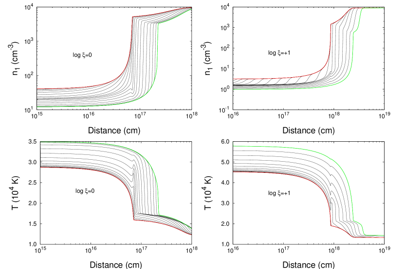
Figure 1: Time dependent simulation for a slab with constant density of $n=10^{4}$ cm^-3 and initial flux of $F_{x}=7.95$ erg cm^-2 s^-1. At $t=0$ s the flux is increased by a factor of 3. The upper and lower panels show the neutral hydrogen density and the gas temperature along the position within the slab, respectively. In both cases, each curve corresponds to the profile at a different moment in time. The initial condition is plotted in red, and the final state of the system is plotted in green.

Figure 1 shows the ionization and temperature time evolutions in hydrogen clouds with two different values of $\xi$. The figure shows that under steady-state conditions the neutral hydrogen density is minimum at the illuminated side of the slab, where the temperature is maximum The ionization and temperature remain relatively constant through the cloud up to a point where most ionizing photons have been absorbed. Then, an IF develops (at 7 – 9$\times 10^{16}$ cm) where the ionization and temperature of the plasma drop sharply. Models for different values of $\xi$ are very similar to each other, but the size of the ionized region scales up with $\xi$.

From the equilibrium state the incident flux is increased suddenly by a factor of 3. We follow the evolution of the system until it reaches an equilibrium state again. As expected, a raise in the flux leads to an increment in the temperature of the gas and in its ionization stage, which consequently decreases the neutral hydrogen fraction.

After the jump in the ionizing flux there is a temporal overshoot in the temperature at the IF, i.e., a sharp increase in temperature followed by a gradual drop to equilibrium values. This is due to the hardening of the ionizing flux that ionizes a largely neutral medium, as the lower energy ionizing photons get absorbed through the ionized region of the cloud. Moreover, a combination of fast moving photoelectrons and relatively few protons make recombination cooling inefficient, resulting in an initial sharp rise in temperature. Later, though, as the plasma becomes highly ionized the recombination cooling rate increases driving the temperature towards an equilibrium value.

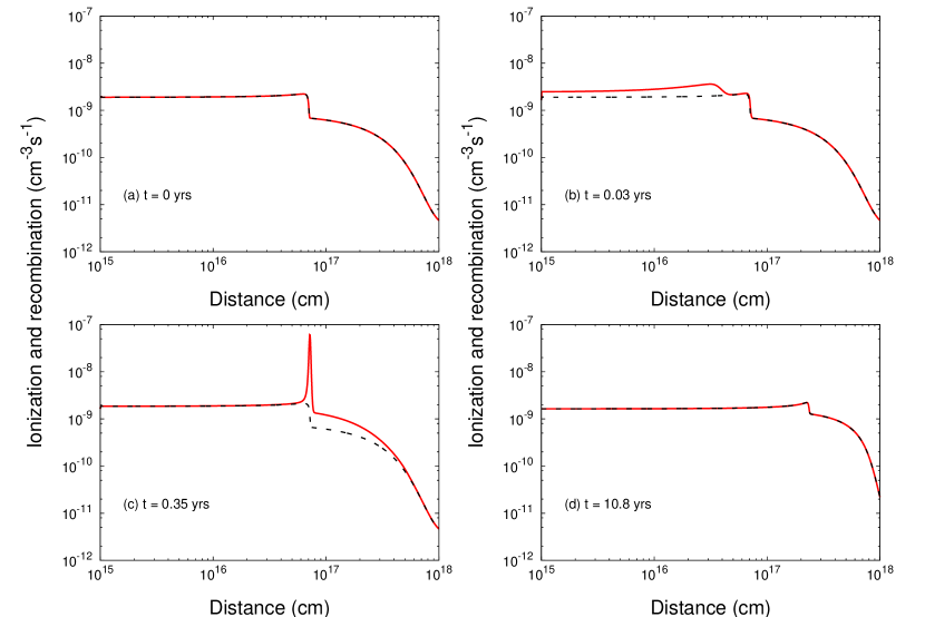
Figure 2: Ionization (solid line) and recombination (dotted line) rates versus depth inside the slab with log $\xi=0$ after a sudden increase of the ionizing flux by a factor of three. The rates are plotted at $t=0$ (initial steady-state conditions), $t=3.4\times 10^{8}$ s (when the slab has reached equilibrium again), and two instants in between.

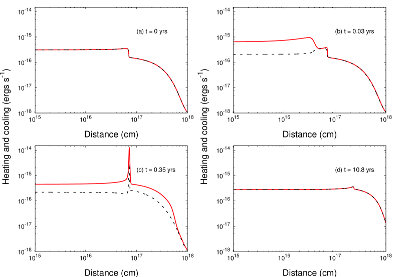
Figure 3: Heating (solid line) and cooling (dotted line) rates versus depth inside the slab with log $\xi=0$ after a sudden increase of the ionizing flux by a factor of three. The rates are plotted at $t=0$ (initial steady-state conditions), $t=3.4\times 10^{8}$ s (when the slab has reached equilibrium again), and two instants in between.

Figures 2 and 3 show the ionization/recombination rates and heating/cooling rates for various time steps after a change in the ionizing radiation field by a factor of three. At $t=0$ and $t>3.4\times 10^{8}$ s ($\sim$10 yrs) the slab is in equilibrium, thus the ionization and heating rates are equal to the recombination and cooling rates, respectively, everywhere in the cloud. In between these times, the figure shows ionization and heating fronts propagating through the cloud leaving the plasma out of equilibrium. At $7.8\times 10^{5}$ s the ionization and heating fronts are found at $3\times 10^{16}$ cm, and the plasma behind these fronts is out of equilibrium. At $t=1.1\times 10^{7}$ s the heating and ionization fronts are seen to reach the IF, where departs from disequilibrium are maxima. Nonetheless, by these times the gas behind the fronts has evolved significantly towards equilibrium.

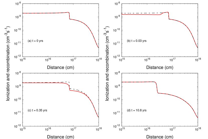
Figure 4: Like Figure 2, but for sudden drop in the ionizing flux by factor three.

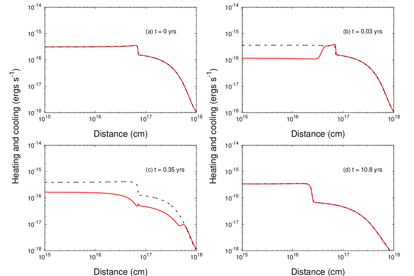
Figure 5: Like Figure 3, but for sudden drop in the ionizing flux by factor three.

The ionization/recombination rates and heating/cooling rates are shown in Figures 4 and 5 for the case when the ionizing continuum is reduced by a factor of three. Cooling and recombination fronts are seen to propagate through the cloud and behind these fronts the plasma evolves towards equilibrium.

4.1.1 Timescales and Rates

In the time-dependent photoionization models shown in Figures 1 the plasmas evolve between two steady-state solutions set by two different values of the ionization parameter. However, the plasma’s behavior is different from a sequence of equilibrium solutions calculated for different ionization parameters at different times. This is because the local conditions at different depths inside the cloud react at different times to the variations in the flux from the source, according to the propagation time. Moreover, the physical conditions evolve at different rates at different depths according to the local timescales for ionization equilibration and temperature equilibration.

Figure 6 shows the propagation, ionization equilibration, and temperature equilibration times versus depth into the slab. It can be seen that fronts that result from sudden increases in the radiation flux travel at constant speed, $\sim 20,000$ km s^-1 ($\sim$MACH 2), from the illuminated face of the slab up to $\sim 3\times 10^{16}$ cm inside the cloud. Beyond this point, the front slows down by orders of magnitude and the propagation time increases non-linearly. In other words, it takes about $\sim$1 year for the radiation front to arrive near the IF, but several hundred years to move across the IF. Clearly, the absolute propagation times are inversely proportional to the magnitude of the flux variation, yet the qualitatively behaviour of the propagation is essentially the same in all cases.

The ionization equilibration time scale depends on the relative change in ionization and the ionization and recombination rates. In steady-state conditions ionization and recombination times are of the order of $\sim$100 yrs, for $T=10^{4}$ K and $n_{e}=10^{4}$ cm^-3. Thus, across the IF, where the neutral hydrogen fraction changes from $\sim$1 to 0, the ionization equilibration time is about 100 yrs. By contrast, before the IF the plasma is nearly fully ionized, thus the relative change in ionization is very small for any increase in the radiation flux and the ionization equilibration time is very short too.

The temperature equilibration time is of the order of a few years in the more ionized segment of the slab and peaks at $\sim$35 yrs across the IF. Interestingly, the temperature equilibration time is longer than the ionization equilibration time in the ionized fraction of the slab, but shorter across the IF.

4.2 Step Flux Function on a Slab in Pressure Equilibrium

Here we investigate the case of a cloud initially in gas pressure equilibrium with its surroundings. Let the pressure at $t=0$ be $P_{o}=4\times 10^{-8}$ dyn cm^-2. For the pressure to be constant across the slab, the gas density increases as $1/T$ from the hotter fraction of the cloud, facing the ionising source, to the neutral region. This means that a sharp rise in density is expected across the IF, where the temperature drops steeply. In the present simulation the IF is originally found at $x\sim 10^{17}$ cm.

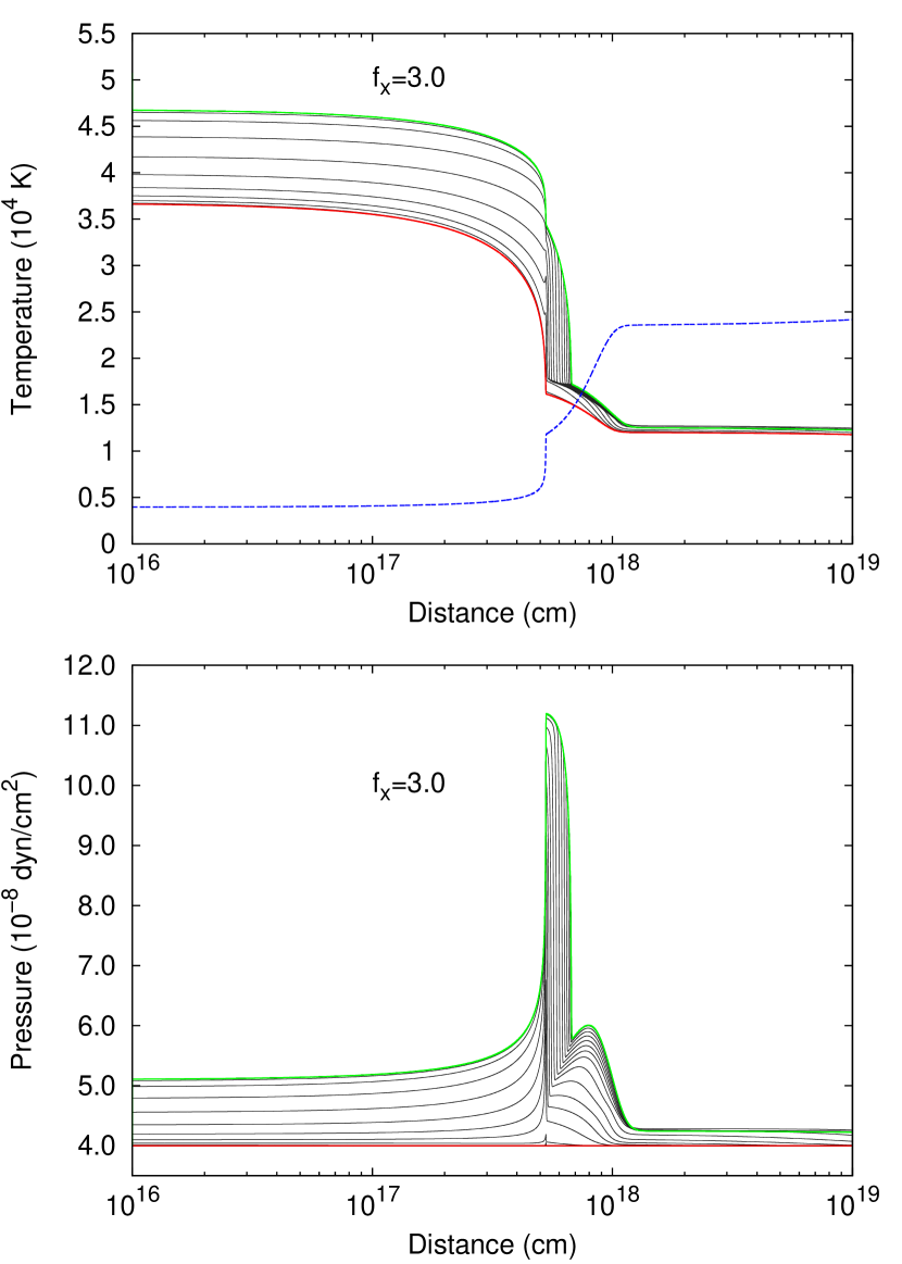
Figure 7: Ionization and temperature for a slab initially in pressure equilibrium at $P_{o}=4\times 10^{-8}$ dyn cm^-2. The initil flux corresponds to log $\xi=0$, which is suddenly increased by a factor of 3 ($f_{x}=3$). The initial condition is plotted in red, and the final state of the system is plotted in green. The black curves depict the physical conditions at different times. The gas density obtained from the pressure equilibrium solution is shown in the upper panel with the dashed-blue line.

In Figure 7 we show the evolution of the temperature and pressure when the ionizing flux is increased by a factor of three ($f_{x}=3$) while the gas density is kept fixed. The increase in flux creates an ionization and thermal front that propagates through the slab and heats the gas beyond the original IF. Thus, the cloud is seen to go out of pressure equilibrium, particularly across the original IF. As a consequence, the variation in the ionizing flux will induce dynamical effects in the cloud. If the thermal front is subsonic the cloud will expand and the density profile of the gas will adjust to maintain equal pressure across the cloud and with its surroundings. Note that if the thermal wave is subsonic in the ionized region the cloud the wave is likely to remain subsonic across the IF. This is because the speed of the front across the IF decreases roughly proportional to $T$, while the sound speed goes as $T^{1/2}$. On the other hand, if the thermal front moves supersonically the gas has no time to adjust itself and strong pressure imbalances, like those seen in Figure 7, will appear. Thus, shocks will be formed in the slab, which can ultimately result in the fragmentation of the cloud (Bautista and Dunn 2010). Either way, variations in the ionizing flux will have important kinematic effects on the cloud.

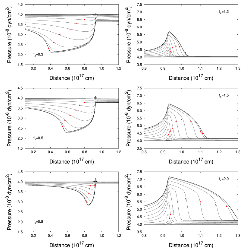
Figure 8: Pressure profiles in the region where the IF is formed (black lines). The red-dots indicate the position of the IF at differemt times. Each panel corresponds to a different flux variation factor $f_{x}$, as indicated.

We further studied front propagations under different conditions. Figure 8 shows the pressure profiles at IFs when the flux is varied by factors of $f_{x}=0.3,0.5,0.8,1.2,1.5$ and $2$. On each curve we identify the inflection point, i.e., the most negative value for $dP/dx$, which we will use as point of reference to follow up the evolution of the front. When the flux is reduced recombination fronts are formed and travel in the direction of the ionizing sourse. Conversely, increased fluxes lead to ionization fronts that travel away from the source.

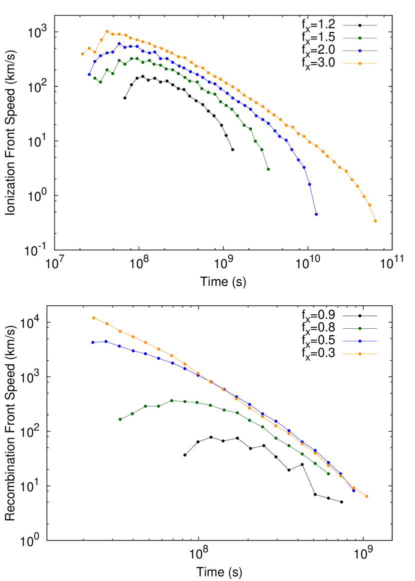
Figure 9: Propagation speed of the IFs (top panel) and recombination fronts (bottom panel). Each curve corresponds to a different flux variation factor $f_{x}$, as indicated in each panel.

Figure 9 shows the speeds of ionization and recombination fronts. It is found that the IFs move forward over long periods of time with speeds proportional to the flux increment (up to $10^{3}$ km s^-1 for $f_{x}=3$). This is consistent with $v_{pro}=F_{x}/H_{H}$ (see Equation 23). On the other hand, recombination fronts propagate with maximum speeds of the order of hundreds of km s^-1 for $f_{x}=0.8$ or smaller. The speed of sound is given by $v_{s}=\sqrt{\gamma p/\rho}$, where $\gamma$ is the adiabatic index, $p$ is the pressure and $\rho$ the mass density of the gas. For an ideal gas $\gamma=5/3$ and temperature range $T=(1-4)\times 10^{4}$ K, $v_{s}=12-24$ km s^-1. Thus, even small variations of the incident flux can induce ionization/recombination fronts that propagate at supersonic speeds.

4.3 Periodically Varying Flux on a Constant Density Slab

In Section 4.2 we showed that equilibratium times at different positions of a slab range by at least an order of magnitude. Thus, there is large variety of astronomical nebulae whose the radiation sources vary periodically on time scales comparable to their equilibration times, e.g., circumstellar nebula around pulsating stars and binary systems. There are also systems, like quasars and AGN, characterized by quasi-periodic variability on all time scales. Thus, it is interesting to look at the general behavior of such systems.

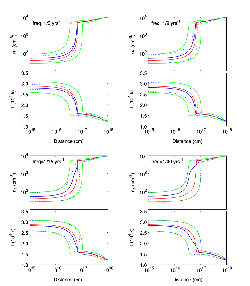
Figure 10: Ionization and temperature solutions for constant density slab subjected to periodically varying fluxes with periods of 3, 9, 15, and 40 yrs. The initial hydrogen density is $10^{4}$ cm^-3, the radiation flux corresponds to log $\xi=0$, and the flux variations are of $f_{x}=\pm 0.5$. The green curves show the steady-state equilibrium conditions at the low and high states of the flux. The red curves depict the steady-state equilibrium solutions for a radiation flux at the media between the low and high states. The blue solid line shows the time average conditions, while the dashed lines show the dispersion in that average.

As discussed in previous sections, slabs with total hydrogen densities of $\sim 10^{4}$ cm^-3 have equilibration times ranging from less than a year to a few decades. Let us consider constant density slabs ionized by step-like periodically varying radiation continua. Figure 10 shows the neutral hydrogen density and temperature for various flux variation periods. These figures show the average physical conditions and their full range of variability. For reference, we also show the steady state solutions for the low and high flux states and the mean conditions between these. Several conclusions can be drawn from this figures:

(1) The time average of the physical conditions is different from the mean of the two steady-state solutions. In general, the cloud tends to be over-ionized with respect to the steady-state solutions for a mean value of the flux. This is because ionization for a given increase in the radiation flux is a faster process (directly proportional to the change in the flux) than recombination when the flux decreases (set by the recombination rate coefficients and the gas density). On the other hand, the time averaged temperature is lower than the mean of steady-state solutions in the ionized region of the cloud.

(2) The dispersion from the time-average of the physical conditions increases with the period of the radiation flux. This is expected because for flux periods shorter than the plasma’s equilibration times the cloud is forced to remain around a non-equilibrium state in-between the two steady state solutions. As the period of the flux variation increases the plasma has time to approach the steady-state solutions. Though, note that the equilibration time across the IF are significantly longer than the ionized region.

(3) Time dependent photoionization leads to much wider IFs than under steady-state conditions. This is due to a combination of strong gradients in equilibration and propagation times across the front. Thus, time-averaged conditions across the IF transition more smoothly from the ionized to neutral regions of the slab than under steady-state conditions. A caveat to this conclusion is that while the average of physical conditions is relatively smooth the absolute instantaneous conditions are not so. It is shown below that the IF exhibits larger variability with respect to average values than anywhere else in the cloud.

Note that the behaviors discussed above are for case of pure hydrogen, optically thin nebulae. Should one expect qualitatively similar effects in more realistic, i.e. chemically heterogeneous and optically thicker, clouds? Adding other chemical elements to the gas is expected to enhance cooling rates and optical depths. These changes are expected to have opposite effects in terms of temporal variability. Larger cooling rates will contribute to reducing the temperature equilibration time. In turn, faster temperature equilibration will tend to drive faster ionization equilibration for neutral species; however, higher ionization stages tend to have smaller photoionization cross sections and for these the ionization equilibration times may be longer. Increasing optical depths would result in reducing effective recombination rates, for example by suppressing Ly$\alpha$ photons hydrogen recombination would be reduced by $\sim 40\%$ to Case B rates which would extend the ionization equilibration times. Moreover, larger optical depths would extend propagation times in general, although the effects would vary along the electromagnetic spectrum and would affect different species selectively. In conclusion, one should expect the effects of periodically varying continuum discussed here to be qualitatively valid in realistic astrophysical nebulae, albeit considerable additional complexity, which deserves additional studies with more complete models.

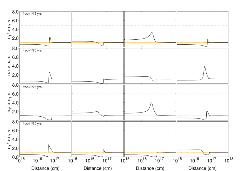
Figure 11: Instantaneous ionization relative to time averaged values for instants along 1000 yr long simulations for various radiation flux variability periods. Here, the radiation flux corresponds to log $\xi=0$ and the amplitude if variations is $f_{x}=\pm 0.5$.

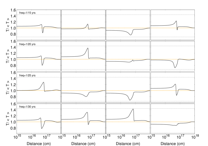
Figure 12: Instantaneous temperature relative to time averaged values for instants along 1000 yr long simulations for various radiation flux variability periods. Here, the radiation flux corresponds to log $\xi=0$ and the amplitude if variations is $f_{x}=\pm 0.5$.

In a gas cloud photoionized by a time-dependent radiation source the physical conditions change asynchronously across the cloud. Full animations of ionization and temperature can be found at http://hea-www.cfa.harvard.edu/$∼$javier/tdp for various flux variability periods. Figures 11 and 12 show a few snapshots of ionization and temperature conditions, normalized to the average values, for simulations run over 1000 yrs. It is seen that even for radiation flux periods as long as 30 yrs the system stays out of equilibrium through the whole duration of the simulation. The ionized region of the slab, that starts from the illuminated face, is seen to vary in sync with the continuum flux. On the other hand, there is a delay between the response across the cloud. Therefore, at any given instant one can find, for example, that while most of the cloud is warmer than the time average, the gas across the IF would be cooler than the average. In general, gas across the IF behaves very differently from the rest of the cloud and exhibits the largest dispersion with respect to time averaged conditions. This is due to the combination of the long propagation time and equilibration times across the IF. Moreover, at no time during the evolution the gas conditions follow a steady-state solution.

5 Conclusions

We have studied the general behavior of time-dependent photoionization models. Here, the energy balance, ionization balance, and radiation transfer equations are considered in their full time-dependent form. These equations are solved for pure hydrogen plasmas subjected to sudden variations in the ionizing radiation field.

Simulations of constant density slabs show the formation of ionization/thermal fronts that propagate through the cloud after a change in the ionizing flux. But, the propagation times and response times to such fronts vary greatly from the illuminated face of the cloud to the IF. Simulations carried out for different degrees of ionization showed that the time evolution of physical conditions in the plasma differs from a sequence of equilibrium solutions.

Our results for slabs initially in pressure equilibrium show that the thermal fronts that propagate through the plasma after a change in the ionizing flux are also pressure fronts, which become particularly pronounced across the IF of the slab. For an increase in the ionizing flux the speed of the thermal front is proportional to the incident radiation flux. Thus, there is no limit for how fast these fronts can propagate. By contrast, a sudden drop in the ionizing flux creates a cooling/recombination front whose speed is determined by the recombination rates. In either case, the present simulations show that these fronts often propagate with supersonic speeds, thus large pressure imbalances are created across the slab. This is expected to have important dynamical effects on the cloud, such as the creation of shocks and cloud fragmentation.

Further, we studied the case of periodic variations in the ionizing flux. It was found that the physical conditions of the plasma have complex behaviors that differ from any steady-state solutions. Moreover, even the time-averaged ionization and temperature are different from any steady-state case. This time average is characterized by over-ionization and a very wide IF with respect to the steady-state solution for a mean value of the radiation flux. Around the time average of physical conditions there is large dispersion in instantaneous conditions, particularly across the IF, which increases with the period of radiation flux. Moreover, the dispersion in physical conditions is asynchronous along the slab due to the combination of non-linear propagation times for thermal/ionization fronts and equilibration times.

Our current description of time-dependent photoionization is simplified owing to the lack of chemical elements other than hydrogen. More realistic models including realistic chemical mixtures and detailed microphysics of multi-level atomic systems will be subject of further publications.

Figure 6: Propagation time (top panel), ionization equilibration time (middle panel), and temperature equilibration time (bottom panel) versus depth within the slab for a plasma with log $\xi=0$ and $f_{x}=3$.

References

- Badnell (2006) Badnell, N. R. 2006, ApJS, 167, 334
- Bautista & Dunn (2010) Bautista, M. A., & Dunn, J. P. 2010, ApJ, 717, L98
- Beck et al. (1995) Beck, H. K. B., Hauschildt, P. H., Gail, H.-P., & Sedlmayr, E. 1995, A&A, 294, 195
- Böttcher et al. (1999) Böttcher, M., Dermer, C. D., Crider, A. W., & Liang, E. P. 1999, A&A, 343, 111
- Carlsson & Stein (2002) Carlsson, M., & Stein, R. F. 2002, ApJ, 572, 626
- Cen (1992) Cen, R. 1992, ApJS, 78, 341
- Davidson & Netzer (1979) Davidson, K., & Netzer, H. 1979, Reviews of Modern Physics, 51, 715
- Dessart & Hillier (2008) Dessart, L., & Hillier, D. J. 2008, MNRAS, 383, 57
- Ercolano et al. (2003) Ercolano, B., Barlow, M. J., Storey, P. J., & Liu, X.-W. 2003, MNRAS, 340, 1136
- Ferland et al. (1998) Ferland, G. J., Korista, K. T., Verner, D. A., Ferguson, J. W., Kingdon, J. B., & Verner, E. M. 1998, PASP, 110, 761
- Ferrara & Giallongo (1996) Ferrara, A., & Giallongo, E. 1996, MNRAS, 282, 1165
- Frank & Mellema (1994) Frank, A., & Mellema, G. 1994, A&A, 289, 937
- Giroux & Shapiro (1996) Giroux, M. L., & Shapiro, P. R. 1996, ApJS, 102, 191
- Harrington (1977) Harrington, J. P. 1977, MNRAS, 179, 63
- Harrington & Marionni (1976) Harrington, J. P., & Marionni, P. A. 1976, ApJ, 206, 458
- Hauschildt et al. (1992) Hauschildt, P. H., Wehrse, R., Starrfield, S., & Shaviv, G. 1992, ApJ, 393, 307
- Hubeny & Lanz (1995) Hubeny, I., & Lanz, T. 1995, ApJ, 439, 875
- Ikeuchi & Ostriker (1986) Ikeuchi, S., & Ostriker, J. P. 1986, ApJ, 301, 522
- Joulain et al. (1998) Joulain, K., Falgarone, E., Pineau des Forets, G., & Flower, D. 1998, A&A, 340, 241
- Kallman & Bautista (2001) Kallman, T., & Bautista, M. 2001, ApJS, 133, 221
- Kozma & Fransson (1998) Kozma, C., & Fransson, C. 1998, ApJ, 496, 946
- Krolik et al. (1981) Krolik, J. H., McKee, C. F., & Tarter, C. B. 1981, ApJ, 249, 422
- Krongold et al. (2007) Krongold, Y., Nicastro, F., Elvis, M., Brickhouse, N., Binette, L., Mathur, S., & Jiménez-Bailón, E. 2007, ApJ, 659, 1022
- Lyu & Bruhweiler (1996) Lyu, C.-H., & Bruhweiler, F. C. 1996, ApJ, 459, 216
- Marten & Szczerba (1997) Marten, H., & Szczerba, R. 1997, A&A, 325, 1132
- Nicastro et al. (1997) Nicastro, F., Fiore, F., Perola, G. C., & Elvis, M. 1997, Mem. Soc. Astron. Italiana, 68, 99
- Nicastro et al. (1999) —. 1999, ApJ, 512, 184
- Osterbrock & Ferland (2006) Osterbrock, D. E., & Ferland, G. J. 2006, Astrophysics of gaseous nebulae and active galactic nuclei
- Perna & Loeb (1998) Perna, R., & Loeb, A. 1998, ApJ, 501, 467
- Richling & Yorke (2000) Richling, S., & Yorke, H. W. 2000, ApJ, 539, 258
- Ricotti et al. (2001) Ricotti, M., Gnedin, N. Y., & Shull, J. M. 2001, ApJ, 560, 580
- Rodriguez-Gaspar & Tenorio-Tagle (1998) Rodriguez-Gaspar, J. A., & Tenorio-Tagle, G. 1998, A&A, 331, 347
- Schmidt-Voigt & Koeppen (1987) Schmidt-Voigt, M., & Koeppen, J. 1987, A&A, 174, 211
- Schwarz et al. (1972) Schwarz, J., McCray, R., & Stein, R. F. 1972, ApJ, 175, 673
- Seager et al. (2011) Seager, S., Sasselov, D. D., & Scott, D. 2011, RECFAST: Calculate the Recombination History of the Universe, astrophysics Source Code Library
- Shapiro et al. (1994) Shapiro, P. R., Giroux, M. L., & Babul, A. 1994, ApJ, 427, 25
- Shapiro & Kang (1987) Shapiro, P. R., & Kang, H. 1987, ApJ, 318, 32
- Tarter et al. (1969) Tarter, C. B., Tucker, W. H., & Salpeter, E. E. 1969, ApJ, 156, 943
- Woods et al. (1996) Woods, D. T., Klein, R. I., Castor, J. I., McKee, C. F., & Bell, J. B. 1996, ApJ, 461, 767