Applications of continuous functions in topological CAD data

Abstract

Most CAD or other spatial data models, in particular boundary representation models, are called “topological” and represent spatial data by a structured collection of “topological primitives” like edges, vertices, faces, and volumes. These then represent spatial objects in geo-information- (GIS) or CAD systems or in building information models (BIM). Volume objects may then either be represented by their 2D boundary or by a dedicated 3D-element, the “solid”. The latter may share common boundary elements with other solids, just as 2D-polygon topologies in GIS share common boundary edges.

Despite the frequent reference to “topology” in publications on spatial modelling the formal link between mathematical topology and these “topological” models is hardly described in the literature. Such link, for example, cannot be established by the often cited nine-intersections model which is too elementary for that purpose. Mathematically, the link between spatial data and the modelled “real world” entities is established by a chain of continuous functions—a very important topological notion, yet often overlooked by spatial data modellers. This article investigates how spatial data can actually be considered topological spaces, how continuous functions between them are defined, and how CAD systems can make use of them. Having found examples of applications of continuity in CAD data models it turns out that of continuity has much practical relevance for CAD systems.

1 Introduction

Spatial data modelling is an important task in almost all engineering applications. Current CAD systems provide spatial models for engineering, and standards have been established to exchange such data between different applications such as STEP for generic engineering and, say, the Industry Foundation Classes (IFC) [1] for the building and construction domain. However, the overall objective of these standardisation efforts towards an integrated multi-user and model-based design environment has not yet been reached [2].

Topology denotes the connectivity between, for example, the rooms of a building and their links like doors, or walls. It also describes the connectivity among these elements. This connectivity can be considered at different levels of detail: A wall may connect two room volumes but it may also be considered a volume connected to each room by its boundary common surface. The “part_of”-relation between these wall-parts and the wall object is already an example of a continuous function. Now, despite the frequent use of the vocabulary “topology” in spatial data modelling publications, only few of them actually use topological methods [3, 4]. Whereas in mathematics continuous functions are an indispensable part of topology and omitting them is just unthinkable, publications on “spatial data” and “topology” are much more frequent than those on “spatial data” and either “continuous function” or “continuous map”. Topology provides an extremely useful mathematical framework for CAD data management for which it might be as important as predicate logic and set theory is for data modelling in general. Note that [5] even proposes topology as a generalisation of graph theory.

This article presents the result of an investigation to locate the open sets, topological spaces, and continuous functions from point set topology within CAD data instances, how continuity can be expressed in terms of the data representations of these topological spaces and which importance continuous functions have therein. Section 3 it introduces the most common generic layout of a topological spatial data model and then introduces “topology” and “continuous function”. Then an idealised spatial modelling “process” transfers “the” topology of the embedding space to the spatial data entities. Section 5 identifies “topology” and “continuous functions” within such data models and thus shows that the “topology” of a CAD model is indeed a mathematical topology which turns the model itself into a space. Such data is linked to the topology of the embedding space $\mathbb{R}^{3}$ by continuous functions which form a “bucket chain” that passes the topology from $\mathbb{R}^{3}$ into the data model. Continuity decides if the spatial model is topologically “correct” and is therefore an interesting consistency constraint. Sections 6 and 7 present other applications of continuity.

As this article focuses on point-set topology other important aspects of data modelling like, for example, semantics, efficency, uncertainty, or object-orientation may not be mentioned here. This does not question their importance but rather means that they are outside the article’s scope.

2 Related work

In contemporary mathematics Topology is considered one of the most fundamental discipline. It also plays an important rôle in spatial data modelling. But many of its possibilities, like the important topological constructions [6, Ch. IV], are currently left unexploited.

“Topological spaces” are, like “vector spaces”, abstractions of the geometrical structures of the Euclidean space $\mathbb{R}^{3}$. After linear algebra has dropped its restriction to $\mathbb{R}^{3}$ due to the work of Cayley [7] it conquered a wide field of applications like finite element computation, or simulation. Topology, too, is not restricted to “spatial” models in $\mathbb{R}^{n}$ the intuitive sense but also covers abstract spatial models [8].

Alexandrov spaces [9] are a particularly important class of topological spaces for computational topology [10] and CAD data modelling. They also generalise undirected graphs which makes topology a sensible supplement of graph theory [5].

The relational model [11] was the first data model based on a strictly formal mathematical theory. Its query “language” is the relational algebra—a definition of the formal semantics of elementary query operators with a deliberate omission of any language syntax [11, p. 21]. A characteristic of this model is its stunning simplicity compared to the database models that have existed so far. This simplicity enabled the development of complex applications, and a general database-design theory [12]. In contrast, [13] identifies unnecessary complexity in the IFC schema. Note that [14] states that from the “progressively increasing complexity” of the future building and construction domain new challenges of BIM will emerge.

The STEP (STandard for the Exchange of Product model data), standardises the exchange of product models [15, 16] and is a basis for CAD models or the IFC. These models combine spatial and domain-specific information and usually are very complex [13, 16]. But even though the IFC cover a broad spectrum of topological modelling elements [17] surprisingly they still seem to lack topological functionality needed: At least Rank e.a. define their own model to access topological information of an IFC model [18]. A very important topological property of a space, or of spatial data, is its homology. Boltcheva e.a. [3] present an efficient algorithm to compute simplicial homology.

An example of topological spaces beyond $\mathbb{R}^{3}$ in the context of relational databases is the theory of acyclic database schemata which converts a database schema into a topological space and tests it for so-called $\alpha$-cycles. This topological property severely affects the efficiency of some database query operations [19].

3 Basic notions

Figure 1 introduces a class diagram of an abstract topological 3D data structure which is frequently used up to minor modifications. This model presents the classical sequence of 3-, 2-, 1-, 0-dimensional entity types where two consecutive entity types are connected by an association into the typical “chain” structure. The length of the sequence corresponds with the dimension of the model and may vary: 2D GIS “polygon topologies” have no Solid class and a 4D-application could append a HyperSolid class to the left.

Figure 1: The classical layout of a “topological” data model—a sequence of classes of spatial entities connected to the typical “cell chain”, or complex, by incidence relations SF, FE, and EV. These induce a relation on SpatialElement.

A vertex usually represents a point in $\mathbb{R}^{n}$ modelled by storing its coordinates. An edge represents a path from a starting vertex to an ending vertex and the data structure relates each edge entity with two vertex entities. Some edges may cycle around a face which then is modelled by a face entity related to its boundary edges by an $n:m$ relationship. Faces may have holes which then partition its boundary edges into components. Some data structures express this partitioning explicitly by providing Loops. We will later see that loops are redundant and can be computed by, say, using [3]. Curiously, arrangements for edges with holes are uncommon. These would then have more than two boundary vertices and will be discussed later. When faces surround a solid that solid is represented by a Solid entity related to its faces by a Solid–Face association.

3.1 Topology

After the following introduction of the topological structure of the embedding space it will be obvious that this structure also applies to spatial data.

The property of the embedding space which leads to its topology is the definition of a distance for every pair of points in a space:

Definition 1 (Metric space).

Let $X$ be a set and $d:X\times X\to\mathbb{R}$ be a function that maps two points $a$ and $b$ to a real value $d(a,b)$. Then $d$ is called a metric on $X$, iff $d$ satisfies the following properties for all $a$, $b$, and $c$ in $X$:

1. $d(a,b)\geq 0$ and $d(a,b)=0\Leftrightarrow a=b$ (non-negativity),

2. $d(a,b)=d(b,a)$ (symmetry),

3. $d(a,b)+d(b,c)\geq d(a,c)$ (triangle inequality).

When $d$ is a metric for $X$ then the pair $(X,d)$ is called a metric space.

The classical example of a metric space is the $n$-dimensional real space $\mathbb{R}^{n}$ with its Euclidean metric

$$d(a,b)=\sqrt{(a_{1}-b_{1})^{2}+\dotsc(a_{n}-b_{n})^{2}}\enspace.$$

Each metric allows a generalisation of open intervals:

Definition 2 (Open ball).

Let $(X,d)$ be a metric space, $c\in X$ an arbitrary (centre) point in $X$ and $r$ an arbitrary positive real number $0<r\in\mathbb{R}$ (radius). Then the set $B(c,r):=\left\{b\in X\mid d(b,c)<r\right\}$ is called an open ball in $(X,d)$.

The open balls in $\mathbb{R}$ are the “open intervals” and $B(c,r)\in\mathbb{R}$ is then usually written as $(c-r,c+r)$. From now on $\bigcup\mathcal{I}$ will be a shorthand notation for $\bigcup_{I\in\mathcal{I}}I$. Every union $\bigcup\mathcal{I}$ of a set $\mathcal{I}$ of open balls will be called an open set in $(X,d)$. The set $\mathcal{T}_{\mathbb{R}^{n}}$ of all open sets in $\mathbb{R}^{n}$ has three fundamental properties which are the defining properties (axioms) of a topology:

Definition 3 (Topology, topological space).

Let $X$ be a set. A set $\mathcal{T}_{X}$ of subsets of $X$ is called a topology for $X$ if it satisfies the following three properties:

1. $\mathbb{X}$ and $\emptyset$ are elements of $\mathcal{T}_{X}$.

2. The union $\bigcup\mathcal{S}$ of every subset $\mathcal{S}$ of $\mathcal{T}_{X}$ is an element of $\mathcal{T}_{X}$.

3. The intersection $A\cap B$ of every two elements $A,B$ of $\mathcal{T}_{X}$ is an element of $\mathcal{T}_{X}$.

Then the pair $\underline{X}:=(X,\mathcal{T}_{X})$ is called a topological space. Every element of $\mathcal{T}_{X}$ is called an open set in $\underline{X}$, and an element of $X$ is called a point in $\underline{X}$.

So any element of any set may be a “point” and a point set can have a many topologies. The above topology $\mathcal{T}_{\mathbb{R}^{n}}$ is called the “natural topology” of $\mathbb{R}^{n}$. But the power set $\mathcal{P}(X)$—the set of all subsets of $X$—is also a topology for $X$ which gives the so-called discrete space $(X,\mathcal{P}(X))$. So there is no “topological property” of an element by itself. This “pluggability” of topologies in mathematics is usually missing in spatial data models where topological properties are often hard-coded into the elements. But because an element may exist in different spaces its topological properties, say, its dimension, may vary therein.

Example 1 (Room connectivity).

Such change of dimension occurs in the “room connectivity graph” of a building (e.g. [20]): A building model is a topological space which contains three-dimensional room objects and two-dimensional connecting doors and other “virtual” passages, say, a door frame without a door. Later this article will introduce the topological subspace. One subspace of a building consists only of its rooms, doors and passages and has dimension one: the rooms therein are 1D and the doors are of dimension zero. The “connectivity graph” is merely its “dual space” where the dimensions of the elements are inverted. Within this space the passages and doors become one-dimensional edges of the connectivity graph each connecting two rooms as its zero-dimensional vertices. This point set topological duality is intimately related to the Poincaré duality from algebraic topology.

3.2 Continuous functions

It is one of the achievements of topology to establish a generic definition of “continuous function”. In calculus real-valued functions $f:\mathbb{R}\to\mathbb{R}$ are called continuous iff (if and only if) “small changes” of the function argument $x$ only lead to “small changes” in the functional value $f(x)$. Its formal definition with the classical $\epsilon$-s and $\delta$-s—distances that represent these small changes—will be omitted here. A generalised “continuity” for data structures with a finite number of elements cannot use a metric and so “small change” must be adapted accordingly: Let $S\subseteq X$ be a set of points of a space $(X,\mathcal{T}_{X})$. A point $p\in X$ is said to be close to $S$ (within $(X,\mathcal{T}_{X})$) if every open set that contains $p$ intersects $S$. The set of all points close to $S$ is denoted by $\operatorname{cl}S$ the closure of $S$. For example, the boundary points of an open interval are not members but close points of the interval, hence $\operatorname{cl}(a,b)=[a,b]$. Using the notion of “close” instead of “small change” gives a purely topological and very illustrative definition of continuous functions:

Definition 4 (Continuous function).

Let $\underline{X}=(X,\mathcal{T}_{X})$ and $\underline{Y}=(Y,\mathcal{T}_{Y})$ be two topological spaces. A function $f:X\to Y$ is called continuous iff for every point $p\in X$ and every set $A\subseteq X$ such that $p$ is close to $A$ in $\underline{X}$ the image point $f(p)$ is close to the image set $f[A]$ in $\underline{Y}$. The fact that $f$ is continuous will be denoted by $f:(X,\mathcal{T}_{X})\to(Y,\mathcal{T}_{Y})$.

So continuous functions respect the “being-close” property within a space. The definition only depends on the topology and forgets any possibly underlying metric. It is equivalent to the calculus definition with the natural topology but it can be applied to every topological space. The above definition is also equivalent to the usual topological definition of continuity:

Theorem 1 (Continuous function).

Let $\underline{X}=(X,\mathcal{T}_{X})$ and $\underline{Y}=(Y,\mathcal{T}_{Y})$ be two topological spaces. A function $f:X\to Y$ is continuous iff for every open set $U\in\mathcal{T}_{Y}$ the pre-image $f^{-1}[U]:=\left\{x\in X\mid f(x)\in U\right\}$ is open in $\underline{X}$.

Now a spatial data modeller must find a data representation of spatial objects in a computer. The following idealised spatial modelling process transfers a physical spatial object into a topological data model and shows that this process is connected by a chain of continuous functions.

4 An idealised spatial modelling process

The idealised spatial modelling “process” does a step-by-step transfer of an assumed “real-world” spatial object from its embedding space $\mathbb{R}^{3}$ into its data representation.

These steps are: First, selecting the (infinite) set of points of the embedding space which are “occupied” by some element of the given object. Then identifying each point set that belongs to a spatial element of that object by partitioning the whole point set into a finite number of parts. This creates a topology for these parts, which is an Alexandrov-topology [9] and hence has a representation as a preordered set, usually a partially ordered set (poset). Finally, for each such element a data entity to represent the corresponding element will be stored together with a relation that represents the poset: Every finite partial order is the transitive and reflexive closure of a directed acyclic graph (DAG).

This section shows that these steps are connected by continuous functions thus exposing continuity as the key consistency rule for “topological correctness” of spatial data.

4.1 Step 1: Carving out the overall shape

The set $\mathbb{R}^{3}$ of the three-dimensional points with its natural topology represents the physical space containing the object in consideration. For simplicity just two unit cubes $[0,1]^{3}$ and $[0,1]^{2}\times[1,2]$ piled atop are considered. This gives a simple specimen of a two-storey “house” as depicted in Figure 2.

The notation $[a,b]$ denotes $\left\{x\in\mathbb{R}\mid a\leq x\leq b\right\}$, the closed interval with $a$ and $b$ as elements. The two cubes are Cartesian products of such intervals.

Figure 2: The “two storey house” with two volumes ($3$-manifolds). Its walls, roof, and slabs are $2$-manifolds, the edges are $1$-manifolds and the vertices are $0$-manifolds.

The selection $H$ of the points occupied by the object gives $H=[0,1]\times[0,1]\times[0,2]$ a prism over a square in the $x,y$-plane. Selecting a set of points from a topological space also returns a topology. So the selection becomes a topological subspace:

Definition 5.

(Subspace) Let $(X,\mathcal{T})$ be a topological space and let $H$ be a subset of $X$. Then the set

$$\mathcal{T}|_{H}:=\left\{H\cap U\mid U\in\mathcal{T}\right\}$$

is a topology for $H$. The topological space $(H,\mathcal{T}|_{H})$ is called the subspace of $H$ in $(X,\mathcal{T})$.

Note that selection is also a relational query operator. The continuous function involved in this construction is the inclusion function

$$i:H\hookrightarrow\mathbb{R}^{3},h\mapsto i(h):=h$$

which relates the domain set $H$ with the range space $\mathbb{R}^{3}$. It is the “engine” that drags the topology from the space to the set: The subspace topology is the unique minimal topology that turns the inclusion function $i$ into a continuous function.

This “handing over topologies” now takes place along a “bucket chain” of functions that connects the real-world space $\mathbb{R}^{3}$ containing the object with the data model instance in the computer. These are all called “topological constructions” and covered, for example, in topology text-books like [6, Ch. IV].

4.2 Step 2: Specifying the features

After turning $H$ into the space $(H,\mathcal{T}|_{H})$ all is ready for the next modelling step: Specify the features the model is composed of. The example on Figure 2 partitions $H$ into 12 vertices, 20 edges, 11 faces, and 2 solids. Here, for simplicity all features are considered manifolds. It will later be diccussed if a manifold assumption can be realistic. “Fat features” would do, too, and walls of non-zero thickness may be connected together by, say, columns the ends of which run into connecting node constructions represented by volume objects. But all features must be non-empty disjoint point sets. For example, a point at such a fat wall’s surface should belong to the wall and not to a room. The “features” are non-empty subsets of $H$ that together cover $H$. A disjoint covering of a set $H$ by non-empty subsets is called a partitioning of $H$ and usually denoted by $H/_{\!\sim}$. Each point $p$ in $H$ has exactly one corresponding point set $[p]\in H/_{\!\sim}$ with $p\in[p]$ which gives another function

$$\pi:H\to H/_{\!\sim},p\mapsto\pi(p):=[p]$$

the natural projection from a single point to its part. The symbol $\sim$ denotes the induced equivalence relation: Two points are equivalent, iff they belong to the same “feature”.

Again, a function connects a space $(H,\mathcal{T}|_{H})$ with a yet unstructured set (of sets) $H/_{\!\sim}$ which now also gets a topology:

Definition 6 (Quotient topology).

Let $(X,\mathcal{T})$ be a topological space and $X/_{\!\sim}$ be a partitioning of $X$. Then the set $\mathcal{T}/_{\!\sim}:=\left\{A\subset X/_{\!\sim}\mid\bigcup A\in\mathcal{T}\right\}$ is called the quotient topology of $\mathcal{T}$ with respect to $\sim$. The topological space

$$(X,\mathcal{T})/_{\!\sim}:=(X/_{\!\sim},\mathcal{T}/_{\!\sim})$$

is called the quotient space of $(X,\mathcal{T})$ with respect to $\sim$.

The quotient topology is the minimal topology such that $\pi$ is continuous. It has taken us one step closer to the spatial data model where each data entity represents a feature of $H/_{\!\sim}$. Note the duality to the first step: Here the topology is passed from a domain space to a range set by $\pi$ whereas the inclusion function passed it from the range to the domain. Accordingly, the quotient topology is the “biggest” topology such that the function $\pi$ stays continuous. So when $i$ was the engine that pulled the topology from $\mathbb{R}^{3}$ into $H$ then $\pi$ is a dual engine that shoves it on to $X/_{\!\sim}$ thus making itself continuous.

Features may be partitioned again, say, by grouping manifolds into fat features. This then gives a “quotient of a quotient” and turns $\pi$ into a “part_of” relation. Repeating this gives a formal model of different levels of detail.

4.3 Step 3: Relations and topologies

Each topological space $(X,\mathcal{T}_{X})$ has an associated preorder relation $\succeq$ on $X$ defined as $b\succeq a\Leftrightarrow a\in\operatorname{cl}\left\{b\right\}$ which is called the specialisation preorder of $(X,\mathcal{T}_{X})$. Conversely, each relation $R$ on a set $X$ defines a topology

$$\mathcal{T}(R):=\left\{A\subseteq X\mid\forall(a,b)\in R:b\in A\Rightarrow a\in A\right\}\enspace.$$ (1)

The preorder $R^{*}$, the transitive and reflexive closure of $R$, is the specialisation preorder of $\mathcal{T}(R)$. Note that bigger relations give smaller topologies: $R\subseteq S\Rightarrow\mathcal{T}(S)\subseteq\mathcal{T}(R)$. We will hence call a relation $R$ finer than $S$ if $R\subseteq S^{*}$ holds. Then $S$ is coarser than $R$. Eqn. 1 indeed satisfies the three axioms and thus denotes a topology: The first is easy to see and the proof of the second and the third are similar. So only the second axiom will be proven here leaving the third axiom to the reader:

Proof.

Let $\mathcal{A}\subset\mathcal{T}(R)$ be an arbitrary set of open sets. Then each satisfies the above property. Assume $a\,R\,b$ and $b\in\bigcup\mathcal{A}$ hold for an arbitrary $b$. By $b\in\bigcup\mathcal{A}$ there exists a set $A\in\mathcal{A}$ which contains $b$. By $a\,R\,b$ the set $A$ also contains $a$ because it is open. Therefore $a$ is in $\bigcup\mathcal{A}$. Hence $\bigcup\mathcal{A}$ is also open. ∎

The similar proof of the third axiom shows that an even stronger property holds: Every set of open sets has an open intersection. The finiteness restriction of axiom three can be dropped which characterises Alexandrov topologies [9]:

Definition 7 (Alexandrov topology).

Let $\underline{X}=(X,\mathcal{T})$ be a topological space. Then $\mathcal{T}$ is called an Alexandrov topology, iff the intersection $\bigcap\mathcal{S}$ of every subset $\mathcal{S}$ of $\mathcal{T}$ is an element of $\mathcal{T}$. Then $\underline{X}$ is called an Alexandrov topological space.

Alexandrov stated, already in 1937, that these spaces (with a restriction called $T_{0}$) are essentially the same as the partially ordered sets $(X,R^{*})$. There are two important properties of Alexandrov spaces: First, a space is an Alexandrov space, iff it can be generated by a relation, and, second, every finite topological space is an Alexandrov space. Interestingly, Sorkin even proposes this topology in theoretical physics as a model for space-time itself because space-time might have an “underlying discreteness” at quantum-level where the assumptions of a $4$-manifold space-time fail [21].

This poset vs. topology equivalence immediately leads to an extremely simple data model which can represent every topology for a finite set:

Definition 8 (Topological data type).

A simple directed graph $(X,R)$ with a set $X$ of elements and a binary relation $R\subseteq X\times X$ is called a topological data type. The topological space $(X,\mathcal{T}(R))$ is the called the topological space represented by $(X,R)$.

$R$ need not be reflexive or transitive but it will be assumed acyclic in this article (to guarantee above mentioned $T_{0}$ restriction) and will be called an incidence relation of $\mathcal{T}(R)$ because special cases of topological data types are called “incidence graphs” [22, p. 395].

The above partitioning of the infinite set $H$ into the finite set $H/_{\!\sim}$ leads to a finite topology $\mathcal{T}/_{\!\sim}$ which then has a minimal incidence relation $Q$ on $H/_{\!\sim}$ such that $\mathcal{T}/_{\!\sim}=\mathcal{T}(Q)$ with $Q^{*}$ as its specialisation preorder. So the final modelling step merely consists in storing a data representation of the finite graph $(H/_{\!\sim},Q)$.

4.4 Step 4: Finally, the data representation

In the final step each feature in $H/_{\!\sim}$ will be represented by a data entity. For example, each vertex $(r_{x},r_{y},r_{z})\in\mathbb{R}^{3}$ gets a unique vertex identifier $n$ and an according entity, say

$$\texttt{Vertex(id:$n$, x:$r_{x}$, y:$r_{y}$ ,z:$r_{z}$)}\enspace,$$

is stored in some data structure. Every edge gets an identifier $\mathit{eid}$ and is stored as Edge(id:$\mathit{eid}$). For each vertex $m$ close to $\mathit{eid}$ the association (Edge.id:$eid$,Vertex.id:$m$) has to be stored, too. Then face entities are stored in Face and, accordingly their “close” relation is stored as a Face–Edge association. Finally, the solids and their corresponding Solid–Face relationships are to be stored. The above example partitioning of $H$ is “docile” in the sense that the “bounded by” relation $Q$ on $H/_{\!\sim}$ can, in fact, be represented by the three associations below SpatialElement but not every partitioning of $H$ has this property.

5 The continuity on spatial data

The above mentioned associations define a relation named “bounded by” on the common superclass SpatialElement. The members of this class will here be denoted by the set $X$ and the incidence relations by one relation $R\subseteq X\times X$. Note that from $(X,R)$ the dimension of each element $x\in X$ can be computed: It is the maximal number $n$ of elements $x_{n},\dotsc,x_{1}\in X$ that can be appended to $x$ in a chain $x\,R\,x_{n}\,R\dotsc R\,x_{1}$. So by unifying all classes into $X$ no information gets lost. Vella, too, proposes the union of edges and vertices of a graph into a set $X$ [5]. Also each chain $x_{a}\,R^{+}\dotsc\,R^{+}\,x_{b}$ of length $m$ can be considered an abstract $m$-simplex $\langle x_{a},\dotsc,x_{b}\rangle$ of an abstract simplicial complex. This has the same homology as $(X,\mathcal{T}(R))$. So the algorithm of [3] can find all loops and shells in $(X,R)$. As mentioned above, explicit loops and shells are redundant.

The function $\sigma:(H/_{\!\sim},\mathcal{T}/_{\!\sim})\to(X,\mathcal{T}(R))$, which maps each feature in $H/_{\!\sim}$ to its representing data entity in $X$, is continuous when each pair $([a],[b])$ of close features has an image pair $(\sigma([a]),\sigma([b]))$ in $R^{*}$ of close data entities. The following statement generalises this:

Theorem 2 (Continuity on topological data types).

Let $(X,R)$ and $(Y,S)$ be two topological data types, and let ${f:X\to Y}$ be a function from $X$ to $Y$. Then $f$ is continuous from $(X,\mathcal{T}(R))$ to $(Y,\mathcal{T}(S))$ iff the image pair $(f(a),f(b))$ of every pair $(a,b)\in R$ is an element of $S^{*}$. Continuity between topological data types will be denoted by $f:(X,R)\to(Y,S)$.

The proof can be found in [23, Thm. 5.6]. The representation $(X,R)$ has the flexibility to also store spaces that result from a “non-docile” partitioning which may result in a relation $R$ that cannot be spread into a chain of, say, three associations. It also allows dynamic change of dimension at run-time.

As $\sigma$ simply carries an incidence relation $Q$ of $(H/_{\!\sim},\mathcal{T}/_{\!\sim})$ to $R^{*}$ it is continuous. But $\sigma$ is a bijection and the inverse function

$$\sigma^{-1}:(X,\mathcal{T}(R))\to(H/_{\!\sim},\mathcal{T}/_{\!\sim})$$

is continuous, too. The features space $(H/_{\!\sim},\mathcal{T}/_{\!\sim})$ and the data space $(X,\mathcal{T}(R))$ created by $(X,R)$ are topologically equivalent or “homeomorphic”. So $(X,R)$ is a topologically consistent representation of $(H/_{\!\sim},\mathcal{T}/_{\!\sim})$.

5.1 The bucket chain of continuous functions

As presented above instances of spatial data are topological spaces and a chain of continuous functions

$$\mathbb{R}^{3}\ \stackrel{{\scriptstyle i}}{{\hookleftarrow}}\ H\ \stackrel{{\scriptstyle\pi}}{{\longrightarrow}}\ H/_{\!\sim}\ \stackrel{{\scriptstyle\sigma}}{{\longrightarrow}}\ X$$

links the entities $X$ of a topological data type $(X,R)$ with the “real world” topological space $\mathbb{R}^{3}$ which contains the object. These functions define the relation $R$ in the data type by passing the topology from left to right.

5.2 Homeomorphism of spatial data

Continuity immediately determines when two instances of spatial data are topologically equivalent or “homeomorphic” just as with every topological space. The definition of homeomorphism needs the identical function on $(X,R)$

$$\operatorname{id}_{(X,R)}:(X,R)\to(X,R),x\mapsto x\enspace.$$

This special case of a continuous inclusion function is trivial but not less important than other mathematical trivialities like the number zero or the empty set.

Definition 9 (Spatial data homeomorphism).

Let $(X,R)$ and $(Y,S)$ be instances of topological data types and let ${f:(X,R)\to(Y,S)}$ and ${g:(Y,S)\to(X,R)}$ be two continuous functions. Then $f$ is called a homeomorphism iff the two function compositions $f\circ g$ and $g\circ f$, with $f\circ g(x)=f(g(x))$ and $g\circ f(x)=g(f(x))$, are the identical functions on $(X,R)$ and $(Y,S)$. Two instances of topological data types are called homeomorphic, iff a homeomorphism between them exists.

It is known to be a hard problem to decide if two given topological data types are homeomorphic: [24] shows that the homeomorphism problem is graph isomorphism complete (and [25] did so two years earlier). The graph isomorphism problem defines a complexity class GI which is supposed to be a bit harder than P but not as hard as NP [26].

6 Applications of continuous functions

Identifying continuity of functions as the formal link between real world spatial objects and their topological data representation might be considered a merely abstract result of no practical relevance. But another practical application of continuity has already been mentioned here: Consistently linking different levels of detail (LoDs)—from the finest, say, “geometric representation” to the corsest “element connectivity”—by a chain of continuous functions, say, “part_of” in a CAD model. This section presents other useful applications of continuity.

It studies continuous functions between two instances of topological data types in an abstract manner, ignoring any “outside” topology of a surrounding world or any other semantics. Having only one universal structure for spatial entities gives the flexibility to map, say, a column volume and its surface at a higher LoD to a simple edge representation of said column at a lower LoD, or, short, to map a mix of 0D, 1D, 2D, and 3D-entities to an $n$D-entity of arbitrary dimension. So continuity between topological data types can become a consistency rule.

Also the topological constructions, like the above presented subspace and quotient space, cover a relationally complete set of topological query operators. These take input spaces and produce output spaces similar to relational algebra which turns input relations to output relations. The input and output spaces are always linked together by continuous functions which define the topology of the query result.

6.1 Continuous foreign key

CityGML’s LoD-references currently permit the coarser object to be of completely different shape and at a completely different location than its finer representation at a higher LoD [27, p. 314]. But objects at different LoDs are topological spaces. So the association between detailed and coarser representation could be restricted by a consistency rule that ensures that the foreign key represents a continuous function from higher to lower LoD. A hypothetical topological RDBMS—which might also become a basis for some database-backed CAD system in the future—could have topological data types $(X,R)$ instead of tables $X$ and should then provide topological DDL-statements like

 CREATE SPACE LoD4
 ( spaceid INTEGER NOT NULL,
   id INTEGER NOT NULL,
   lod3space INTEGER,
   lod3id INTEGER,
   yaAttribute YATYPE,
   ...
   PRIMARY KEY(spaceid, id),
   CONTINUOUS FOREIGN KEY
     (lod3space,lod3id)
     REFERENCES LoD3(spaceid,id),
   ...);

with the CONTINUOUS consistency constraint on foreign keys. A foreign key from one relation $R$ into another relation $S$ defines a function $f:R\to S$ that maps a referring tuple $r\in R$ to a referred tuple $f(r)\in S$. When $R$ and $S$ are spaces the database administrator could then establish a continuity restriction on $f$ whenever he needs it. The later example of a topologically integrated detail library will use this continuity constraint.

6.2 Constructions and queries

Resuming the modelling steps shows that, first, there was a “selection” of some points from the embedding topological space which returned another topological space, the subspace. Then the selected points have been mapped into a set of features by a “projection” which also not only converted points into features but additionally produced a topology for them. So these are already two analogs for relational query operators which leads to the question how relational algebra could act on a CAD model.

A relationally complete set of query operations for topological data types can be found in [23]. Table 1 lists some basic operators of relational algebra, their corresponding topological constructions, and the functions involved. Each query operator has functions that connect the input tables with the result table. These functions define the query result topology either as a “final” topology when the functions map to the result, or as an “initial” topology when the functions map the from the result to the input. It is always the topology that most resembles all input topologies but still keeps all linking functions continuous. A first experimental prototype of a topological relational algebra implemented by the author can be found on http://pavel.gik.kit.edu.

Operation	Construction	Function(s)
selection	subspace	$i:\sigma_{\Theta}(X)\hookrightarrow Xs$
projection	final space	$\pi_{\mathcal{A}}:X\to\pi_{\mathcal{A}}(X)$
union	pasting	$\check{\imath}_{X}:X\hookrightarrow X\cup Y$
		$\check{\imath}_{Y}:Y\hookrightarrow X\cup Y$
intersection	pullback	$\hat{\imath}_{X}:X\cap Y\hookrightarrow X$
		$\hat{\imath}_{Y}:X\cap Y\hookrightarrow Y$
Cartesian product	product space	$\pi_{X}:X\times Y\to X$
		$\pi_{Y}:X\times Y\to Y$

Table 1: Relational query operators, their corresponding topological constructions, and the continuous functions involved. The functions are either $f:X\to\texttt{op}(X,\dotsc)$ from a query input table $X$ to the query output table $\texttt{op}(X,\dotsc)$ or $g:\texttt{op}(X,\dotsc)\to X$ from the output to an input. When that arrow points to the output, the result topology is called a “final” topology, otherwise it is called “initial”. $i$, $\check{\imath}$, and $\hat{\imath}$ are inclusion functions.

The following discussion of Cartesian Product and join illustrates how topological constructions act on the relational representation of topological spaces.

6.2.1 Cartesian product and join

The topological analog for the Cartesian product is the product space with its important practical application in CAD that it topologically generalises extrusion. Let $(X,R)$ and $(Y,S)$ be two spatial data types, say, an axis $X$ and a profile $Y$. Then the Cartesian product is the set $X\times Y$ of entity-pairs $ts$ where $t$ is in $X$ and $s$ is in $Y$. The functions that link input with output are the two projections $\pi_{X}:X\times Y\to X,ts\mapsto t$ and $\pi_{Y}:X\times Y\to Y,ts\mapsto s$. A maximal relation for $X\times Y$ that makes both projections continuous is made up of two components: A “horizontal” part $\mathit{RY}$ that creates $Y$ copies of $R$ each “tagged” by an element of $Y$ and a “vertical” part $\mathit{XS}$ that creates $X$ copies of $S$ each “tagged” by an element of $X$. The vertical part will be defined as

$$\mathit{XS}:=\left\{(xa,xb)\mid x\in X,a\,S\,b\right\}\enspace.$$

Accordingly the “horizontal” part is

$$\mathit{RY}:=\left\{(cy,dy)\mid c\,R\,d,y\in Y\right\}\enspace.$$

The union $\mathit{XS}\cup\mathit{RY}$ is a binary relation for $X\times Y$ that creates the product space topology [23]. So the Cartesian product space is generated by

$$(X,R)\times(Y,S):=(X\times Y,\,\mathit{XS}\cup\mathit{RY})\enspace.$$

Besides, it shall be mentioned that the topological dimension of spatial data (also called “Krull dimension” [28, p. 5]) of the product space is the sum of the dimensions of the input spaces. The Cartesian product space of, say, two instances of a 3D data model will result in a 6D product space and would not fit into the restricted data model from Figure 1.

A relational $\Theta$-join can now be formally defined as the subspace obtained by selecting the entity-pairs which satisfy the join-predicate $\Theta$ from the product space

$$(X,R)\Join_{\Theta}(Y,S):=((X,R)\times(Y,S))|_{\sigma_{\Theta}(X\times Y)}$$

using the selection operator $\sigma$.

7 More applications of continuity

After having seen how continuous functions can define basic query operators two not-so-basic applications of topological constructions will be presented here.

7.1 A topological detail library

The following construction is called fibre product in topology and corresponds with the relational equi-join. The LoD-sequence of spaces—each a model of the same real-world object at a different level of detail—is linked by continuous functions “part_of” where each maps a finer object to a coarser representation. But engineering design often starts at the coarse side with sketchy design ideas that are later refined. It is also common in CAD-systems to define complex “macro”-objects of frequently reused parts to be placed into a drawing. The following topological construction can do both:

Definition 10 (Fibre product).

Let $(X,\mathcal{T}_{X})$, $(Y,\mathcal{T}_{Y})$, and $(I,\mathcal{T}_{I})$ be topological spaces and $f:(X,\mathcal{T}_{X})\to(I,\mathcal{T}_{I})$ and $g:(Y,\mathcal{T}_{Y})\to(I,\mathcal{T}_{I})$ be two continuous functions. Then the space

$$(X,\mathcal{T}_{X})\times_{I}(Y,\mathcal{T}_{Y}):=\sigma_{f=g}((X,\mathcal{T}_{X})\times(Y,\mathcal{T}_{Y}))$$

is called the fibre product space of $f$ and $g$. $\sigma_{P}(S)$ is the selection $\left\{s\in S\mid s\text{ satisfies }P\right\}$.

It is the space of all entity-pairs $xy$ from $X\times Y$ where $f(x)=g(y)$ holds. When $X$ and $Y$ are database tables with attributes $f$ and $g$ then $X\times_{I}Y$ is the equi-join $X\Join_{f=g}Y$.

The use of macro objects in a CAD drawing can be considered a fibre product: The set of the macro-names is a discrete space $I$ of identifiers. The locations in a drawing where such macro objects are used is another discrete space $X$. The use of macros establishes a function $f$ from the locations to the identifiers. This function is continuous because of its discrete domain. The set of all macros $Y$ is a so-called sum-space: a disjoint sum of topological spaces—one subspace per macro—each indexed by its macro identifier. Also the function $g$ that maps macro elements to macro identifiers is continuous if there is no connectivity between two different macros. Now the insertion of copies of macros into the drawing corresponds to the fibre product of the two continuous functions “macro-use” $u$ and “macro naming” $p$ which have a common range space, the discrete space $I$ of macro identifiers.

Until now this was just a formal overkill but when the macro names get a topology and the macro objects space is coarsened, this turns into a system of a topologically integrated library of parts that are chosen and linked together by a coarser sketchy drawing and both together produce the detailed plan.

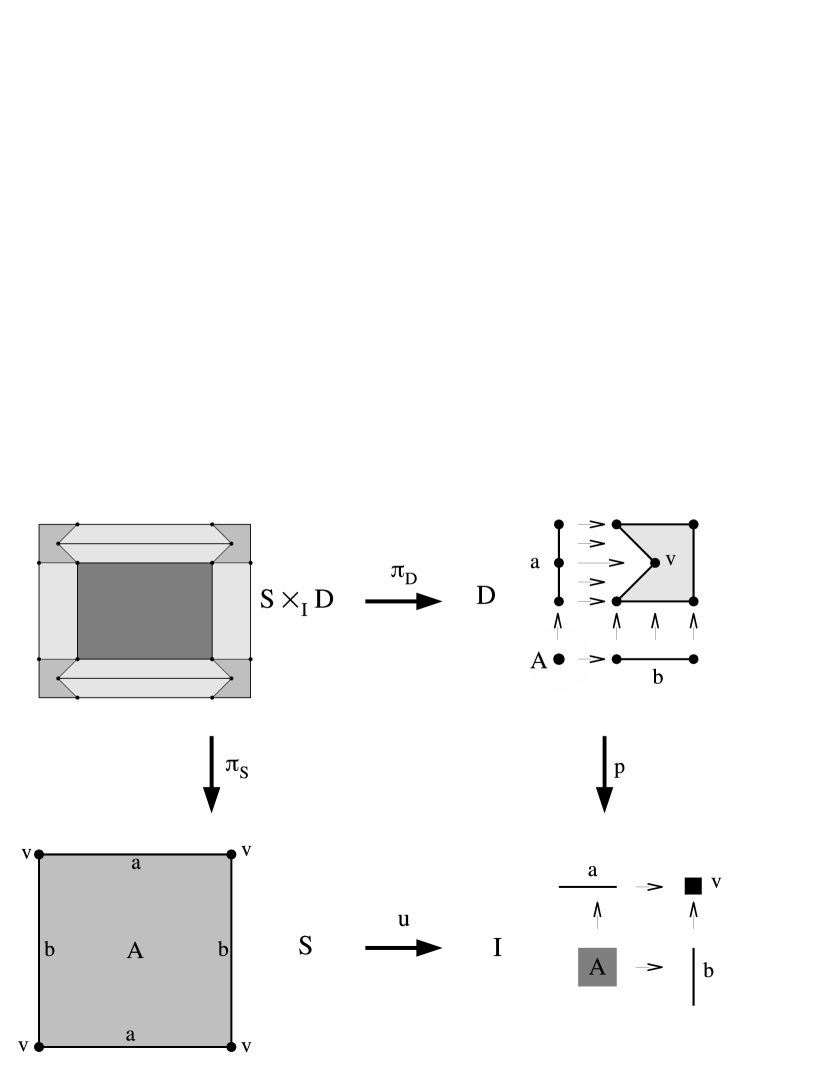
Figure 3: The fibre product space $S\times_{I}D$ of the continuous functions ${p:D\to I}$ and ${u:S\to I}$ (the detail usage) “topologically integrates” the space of details $D$, the space of the detail index $I$ and the sketch $S$ into a more detailed space.

The following is a simple 2D-example but the intended application is 3D CAD: Figure 3 shows a sketchy drawing $S$ on the lower left hand side and a space of some details $D$ on the upper right hand side. Both are topological spaces with continuous functions $u:S\to I$ and $p:D\to I$ that map into a common index space $I$. $u$ stands for “usage” and denotes which detail from the detail library $p:D\to I$ shall be used. The “usage”-values of $u$ are depicted in $S$: The area element “uses” $A$, the $u$-value of the two horizontal lines is $a$, that of the vertical lines it is $b$, and so on. The same is true for the $p$-values in $D$. The little arrows in $D$ and $I$ indicate the topological incidence relation between the single detail entities. Therefore the details are no longer a disjoint sum. For example, detail $a$ consists of five entities of which the middle vertex is “close” to the vertex in the notch of detail $v$.

The detail of name $x\in I$ is the subspace of the elements in $D$ that map to $x$, hence the pre-image $p^{-1}(x)$ of $x$ under $p$. Pre-images of points are also called “fibres” and therefore this construction is named “fibre product”. For example, the detail $a$ is the sequence of the three vertices connected by two edges in the upper left corner of $D$.

The fibre product space $S\times_{I}D$ is generated be these two functions: It is the topological equi-join $S\Join_{u=p}D$ depicted in the upper left corner of Figure 3. For example, the upper horizontal “wall” is an extrusion of the detail $a$ along the upper horizontal edge and it seamlessly connects to the notch of the vertex detail $v$. This operation has some interesting features for 3D CAD and CAE design:

• The details are a topological generalisation of “macro” objects in CAD.

• It is possible to specify the connectivity between details in a uniform manner.

• The detail library, the continuous function $p$, establishes consistency rules on how details can be used and which details can be “compatibly” connected.

• A user working on the drawing $S$ can only select his details from $I$, as long as his “detail use”-function $u$ remains continuous. The continuity constraint prohibits incompatible connections and thereby again advocates for continuity as a consistency rule.

• Details can be placed at singular locations like traditional macro objects but can also be “extruded” along extended objects: A two-dimensional profile can be extruded along a one-dimensional axis whereas a one-dimensional sequence of wall-layers can be extruded along a 2D wall face to generate a 3D-wall sandwich element. All these extrusions generate 3D-objects and the components’ dimensions sum up to 3.

There are still open questions: For example, a naive use of the pullback can return a topology that is too coarse for practical applications, hence, some “refinement” of the concept is still necessary. But it surely will be the essential ingredient of any topologically integrated detail library application for CAD systems.

7.2 Intersection

Until now only combinatorial topological operations have been considered. The computation of the intersection space that results in overlaying geometrically embedded spatial data is another important operation. In GIS, for example, this “overlay” is often used to carry out combined spatial data analysis.

Let there be a predicate $\Theta$ that tells for two given elements $a$ and $b$, each from one space, if they geometrically intersect. Iff they intersect $\Theta(a,b)$ is true. An algorithm for $\Theta$ on $n$D-polytope complexes is sketched in [29].

With two topological data types $(X,R)$ and $(Y,S)$ and such an “intersects” predicate $\Theta$ the intersection space is the $\Theta$-Join

$$(X,R)\Join_{\Theta}(Y,S):=\sigma_{\Theta}((X,R)\times(Y,S))\enspace.$$

It consists of all pairs of elements that have a geometrical intersection. Clearly, the intermediate Cartesian product space computation is expensive and should be avoided in practice. Codd calls this emphasis of avoiding the Cartesian product wherever possible its “de-emphasising” [30]. Similar to the fibre product the join also gets a topology for these pairs. Figure 4 gives an example. Note that by explicitly storing $\Theta$ into an association $\Theta\subseteq X\times Y$ the three items $(X,R)$, $(Y,S)$, and $\Theta$ realise the $Q$-Complex proposed in [31].

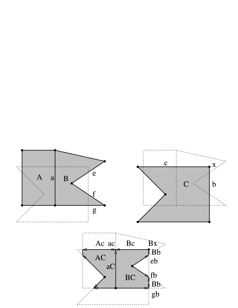
Figure 4: The intersection space of two spaces of geometrically intersecting entities. Topologically it is the two-dimensional subspace of intersecting cell pairs within the four-dimensional product space. The combinatorial “close-to” relation computed by the relational query operators indeed matches the metric “close-to” from the embedding of the intersection. The two projections from the intersection back to the intersecting spaces are continuous.

Some elements from the two intersected spaces in Figure 4 show how the $\Theta$-join computes the topology. The left-hand side space contains two faces $A$ and $B$, eight edges—among which four are labelled $a$, $e$, $f$, and $g$—and seven vertices. The right-hand side space is made of only one face $C$ bounded by five edges where two are labelled $b$ and $c$, and five vertices among one is named $x$. The incidence relations for the named entities are

$$R=\left\{(A,a),(B,a),(B,e),(B,f),(B,g)\right\}$$

and

$$S=\left\{(C,c),(C,b),(c,x),(b,x)\right\}\enspace.$$

The pair $(C,x)$, which denotes that vertex $x$ is close to face $C$, is in $S^{+}$, the transitive closure of $S$. The intersections of the elements in $X\supset\left\{A,B,a,e,f,g\right\}$ with those in $Y\supset\left\{C,b,c,x\right\}$ can be decided by feeding each pair into $\Theta$. For example, $\Theta(A,c)$ returns true and $\Theta(A,b)$ returns false. The following 24-intersections matrix depicts all pairs of intersecting named entities, that is, all $pq$ where $\Theta(p,q)$ is true.

	$A$	$B$	$a$	$e$	$f$	$g$
$C$	$AC$	$BC$	$aC$	$eC$	$fC$	$gC$
$b$		$Bb$		$eb$	$fb$	$gb$
$c$	$Ac$	$Bc$	$ac$
$x$		$Bx$

In the product space the pair $aC$ is “close to” $AC$ because $a$ is close to $A$ and for all elements $q$ in the other space the pair $(A,a)$ in $R$ is converted into $(Aq,aq)$. As $C$ is one such $q$ the incidence $(AC,aC)$ belongs to the incidence relation of the product space. Conversely, the pair $(C,c)$ in the right-hand side incidence relation has been turned into the incidences

$$\{ (AC,Ac),(BC,Bc),(aC,ac),$$

$$(eC,ec),(fC,fc),(gC,gc),\dotsc\}$$

telling, for example, that $Bc$ is close to $BC$. From that four-dimensional product space the predicate $\Theta$ selects the intersecting entity pairs. Together with its subspace incidence relation this gives a two-dimensional result space. The projections from the intersection back into the input are continuous functions: The left hand side projection takes, for example, the incident elements $AC$ and $Ac$ to $A$ and so by ${\pi_{X}(AC)=A=\pi_{X}(Ac)}$ this pair satisfies the continuity condition for the projection
${\pi_{X}:X\Join_{\Theta}Y\to X}$. The right hand side projection takes $AC$ to $C$ and $Ac$ to $c$ and so $(\pi_{Y}(AC),\pi_{Y}(Ac))=(C,c)\in S$. Therefore the pair also satisfies the continuity condition for the other projection $\pi_{Y}:X\Join_{\Theta}Y\to Y$.

Interestingly the edge $Bb$ has four vertices $Bx$, $eb$, $fb$, and $gb$. So $Bb$ became an edge with a hole. This is how the $\Theta$-join produces this boundary of $Bb$: The involved entities are $B$, $e$, $f$, and $g$ in $(X,R)$ and $b$, and $x$ in $(Y,S)$. The involved incidence relations are

$$\left\{(B,e),(B,f),(B,g)\right\} \subset R$$

$$\text{~{}and~{}}\left\{(C,b),(b,x)\right\} \subset S\enspace.$$

The following 17-products-matrix shows the incidence relation for the Cartesian product space of the subspace near $Bb$. An entry which depicts a non-intersection is stroked out and pairs where $Bb$ is at the left-hand side are highlighted in bold face:

	C	b	x	(C, b)	(b, x)
B				(BC, Bb)	(Bb, Bx)
e				(eC, eb)	(eb, ex)
f				(fC, fb)	(fb, fx)
g				(gC, gb)	(gb, gx)
(B, e)	(BC, eC)	(Bb, eb)	(Bx, ex)
(B, f)	(BC, fC)	(Bb, fb)	(Bx, fx)
(B, g)	(BC, gC)	(Bb, gb)	(Bx, gx)

This gives the incidences $(Bb,Bx)$, $(Bb,eb)$, $(Bb,fb)$, and $(Bb,gb)$, hence $Bx$, $eb$, $fb$, and $gb$ are in the boundary of $Bb$. They are vertices because they do not occur as a left-hand side element in an incidence and having an empty boundary characterises vertices in the topological model. Note that $eb$ is a zero-dimensional vertex in the $\Theta$-join space but it was a two-dimensional element in the intermediate product space because it is the pair of the two edges $e$ and $b$, each of dimension 1, and in the product space the dimensions of elements add. This shows how the generic concept of a topological data type allows to dynamically shift the dimension upper bound up and down as necessity arises.

8 Conclusion and outlook

The research which rôle continuous functions might play in CAD data models has shown that they link the embedding space with the spatial data. These data models are topological spaces, and so continuity is well-defined for spatial data. It has been demonstrated how continuity of functions can be a versatile tool for spatial data modelling and can be used as a consistency rule. Continuity also suggests relaxing the current strict-typed topological models with their classical volume-face-edge-vertex sequences and have a closer look at their common generalisation SpatialObject.

Topological constructions are based on continuity and it has been shown that all basic query operators of relational algebra have corresponding topological query operators for spatial data. So the relational representation not only enormously simplifies spatial data modelling but also adds expressive power to spatial data management. This topological relational algebra could be part of a framework for future database-backed CAD systems. In particular, the fibre product has been identified as an extremely promising topological construction for CAD and CAE applications.

To wrap it up, it has been shown that the importance of continuous functions in topology reflects onto CAD modelling, and the potentials of mathematical topology have been demonstrated here to go far beyond giving predicate names to intersection patterns. In addition to providing a theoretical framework and to its relationally complete set of query operators, topology still offers many concepts that just wait for being harvested from literature and used in future CAD and CAE applications.

9 Acknowledgements

This work was funded by the German Research Foundation (Deutsche Forschungsgemeinschaft DFG) with research grant BR2128/12-2. The author thanks Patrick Erik Bradley for valuable remarks and discussions on this topic.

References

-
[1]
buildingSMART International Ltd.,
IFC
2x Edition 3 Technical Corrigendum 1, [online] (2007).
URL http://www.buildingsmart-tech.org/ifc/IFC2x3/TC1/html/i%ndex.htm -
[2]
M. P. Nepal, S. Staub-French, R. Pottinger, A. Webster,
Querying a building information model for construction-specific spatial
information, Advanced Engineering Informatics 26 (4) (2012) 904 – 923.
doi:10.1016/j.aei.2012.08.003.
URL http://www.sciencedirect.com/science/article/pii/S14740%34612000778 -
[3]
D. Boltcheva, D. Canino, S. M. Aceituno, J.-C. Léon, L. D. Floriani,
F. Hétroy,
An
iterative algorithm for homology computation on simplicial shapes,
Computer-Aided Design 43 (11) (2011) 1457 – 1467.
doi:10.1016/j.cad.2011.08.015.
URL http://www.sciencedirect.com/science/article/pii/S00104%48511002144 -
[4]
S. Raghothama, Constructive
topological representations, in: Proceedings of the 2006 ACM symposium on
Solid and physical modeling, SPM ’06, ACM, New York, NY, USA, 2006, pp.
39–51.
doi:10.1145/1128888.1128894.
URL http://doi.acm.org/10.1145/1128888.1128894 -
[5]
A. Vella, A fundamentally topological
perspective on graph theory, Ph.D. thesis, University of Waterloo (2005).
URL http://hdl.handle.net/10012/1033 - [6] O. Y. Viro, O. A. Ivanov, N. Y. Netsvetaev, V. M. Kharlamov, Elementary Topology: Problem Textbook, AMS, 2008.
-
[7]
P. G. Tait,
Obituary on James Clerk Maxwell, in: Proceedings of the Royal Society of
Edinburgh, Vol. 10, The Royal Society of Edinburgh, 1878-80, pp. 331–339.
URL http://www.clerkmaxwellfoundation.org/JCMObitbyPGTait20%08_2_22.pdf -
[8]
D. Braha, Y. Reich,
Topological structures for
modeling engineering design processes, Research in Engineering Design 14 (4)
(2003) 185–199.
doi:10.1007/s00163-003-0035-3.
URL http://dx.doi.org/10.1007/s00163-003-0035-3 -
[9]
P. Alexandroff, Diskrete Räume,
Matematiećeskij Sbornik 44 (2) (1937) 501–519.
URL http://mi.mathnet.ru/eng/msb5579 -
[10]
F. G. Arenas,
Alexandroff spaces, Acta Math. Univ. Comenianae 68 (1) (1999) 17–25.
URL http://www.emis.ams.org/journals/AMUC/_vol-68/_no_1/_ar%enas/arenas.pdf -
[11]
E. F. Codd, A
relational model of data for large shared data banks, Commun. ACM 26 (1)
(1983) 64–69.
doi:10.1145/357980.358007.
URL http://dl.acm.org/citation.cfm?doid=357980.358007 -
[12]
E. F. Codd, Data models in
database management, SIGMOD Rec. 11 (2) (1980) 112–114.
doi:10.1145/960126.806891.
URL http://doi.acm.org/10.1145/960126.806891 -
[13]
R. Amor, Y. Jiang, X. Chen,
Bim in 2007 -
are we there yet?, in: Bringing ITC knowledge to work, CIB W78, Maribor,
Slovenia, 2007, pp. 159–162.
URL http://www.cs.auckland.ac.nz/~trebor/papers/AMOR07B.pdf -
[14]
A. Watson,
Digital buildings – challenges and opportunities, Advanced Engineering
Informatics 25 (4) (2011) 573 – 581.
doi:10.1016/j.aei.2011.07.003.
URL http://www.sciencedirect.com/science/article/pii/S14740%34611000516 - [15] G. Augenbroe, Combine 2 final report, Tech. rep., CEC-JOULE Report, Brussels (1995).
- [16] C. M. Eastman, Building Product Models: computer environments supporting design and construction, CRC Press LLC, Boca Raton, Florida, 1999.
-
[17]
N. Paul,
Basic topological notions and their relation to bim, in:
J. Underwood, U. Isikdag (Eds.), Handbook of Research on Building Information
Modeling and Construction Informatics, Information Science Reference, 2010,
pp. 451–472.
URL http://www.igi-global.com/chapter/basic-topological-not%ions-their-relation/39483 -
[18]
E. Rank, R. Romberg, A. Niggl, H.-J. Bungartz, R.-P. Mundani,
Volumenorientierte
modellierung als grundlage einer vernetzt-kooperativen planung im
konstruktiven ingenieurbau, in: U. Rüppel (Ed.), Vernetzt-kooperative
Planungsprozesse im Konstruktiven Ingenieurbau, Springer Berlin Heidelberg,
2007, pp. 295–319.
URL http://dx.doi.org/10.1007/978-3-540-68104-5_16 -
[19]
R. Fagin, Acyclic database
schemes (of various degrees): A painless introduction, in: G. Ausiello,
M. Protasi (Eds.), CAAP’83, Vol. 159 of Lecture Notes in Computer Science,
Springer, 1983, pp. 65–89.
doi:10.1007/3-540-12727-5\_3.
URL http://dx.doi.org/10.1007/3-540-12727-5_3 -
[20]
C. S. Jensen, H. Lu, B. Yang,
Graph model based indoor
tracking, in: Proceedings of the 2009 Tenth International Conference on
Mobile Data Management: Systems, Services and Middleware, MDM ’09, IEEE
Computer Society, Washington, DC, USA, 2009, pp. 122–131.
doi:10.1109/MDM.2009.23.
URL http://dx.doi.org/10.1109/MDM.2009.23 -
[21]
R. Sorkin, Finitary substitute for
continuous topology, International Journal of Theoretical Physics 30 (7)
(1991) 923–947.
doi:10.1007/BF00673986.
URL http://dx.doi.org/10.1007/BF00673986 -
[22]
E. Brisson, Representing geometric
structures ind dimensions: Topology and order, Discrete & Computational
Geometry 9 (1) (1993) 387–426.
doi:10.1007/BF02189330.
URL http://dx.doi.org/10.1007/BF02189330 -
[23]
P. E. Bradley, N. Paul,
Using the
relational model to capture topological information of spaces, The Computer
Journal 53 (1) (2010) 69–89.
doi:10.1093/comjnl/bxn054.
URL http://comjnl.oxfordjournals.org/content/53/1/69.abstra%ct -
[24]
N. Paul,
Topologische
datenbanken für architektonische räume, Ph.D. thesis,
Universität Karlsruhe (2008).
URL http://digbib.ubka.uni-karlsruhe.de/volltexte/100000784%3 -
[25]
A. Bretto, A. Faisant, T. Vallée,
Compatible topologies on graphs: An application to graph isomorphism problem
complexity, Theoretical Computer Science 362 (2006) 255–272.
doi:10.1016/j.tcs.2006.07.010.
URL http://www.sciencedirect.com/science/article/pii/S03043%97506004221 -
[26]
C. M. Hoffmann,
Group-theoretic algorithms and graph isomorphism, Springer, 1982.
doi:10.1007/3-540-11493-9.
URL http://link.springer.com/book/10.1007/3-540-11493-9/pag%e/1 -
[27]
P. Oosterom, J. Stoter,
5d data modelling: Full
integration of 2d/3d space, time and scale dimensions, in: S. Fabrikant,
T. Reichenbacher, M. Kreveld, C. Schlieder (Eds.), Geographic Information
Science, Vol. 6292 of Lecture Notes in Computer Science, Springer, 2010, pp.
310–324.
doi:10.1007/978-3-642-15300-6\_22.
URL http://dx.doi.org/10.1007/978-3-642-15300-6_22 - [28] R. Hartshorne, Algebraic Geometry, Vol. 52 of Graduate texts in mathematics, Springer, 1977.
- [29] N. Paul, M. Menninghaus, Signed simplicial decomposition and intersection of n-d-polytope complexes, in: Proceedings of the 24rd European Conference Forum Bauinformatik, 2012, pp. 103–110, bochum, Germany.
-
[30]
E. F. Codd, The Relational Model
for Database Management: Version 2, repr. with corr. Edition,
Addison-Wesley, 1990.
URL http://dl.acm.org/citation.cfm?id=77708 -
[31]
L. Zeng, Y.-J. Liu, S. H. Lee, M. M.-F. Yuen,
-complex: Efficient non-manifold boundary representation with inclusion
topology, Computer-Aided Design 44 (11) (2012) 1115–1126.
doi:10.1016/j.cad.2012.06.002.
URL http://www.sciencedirect.com/science/article/pii/S00104%48512001285