Rotational bands in the continuum illustrated by ⁸Be results

Abstract

We use the two-alpha cluster model to describe the properties of ⁸Be. The rotational energy sequence of the $(0^{+},2^{+},4^{+})$ resonances are reproduced with the complex energy scaling technique for Ali-Bodmer and Buck-potentials. However, both static and transition probabilities are far from the rotational values. We trace this observation to the prominent continuum properties of the $2^{+}$ and $4^{+}$ resonances. They resemble free continuum solutions although still exhibiting strong collective rotational character. We compare with cluster models and discuss concepts of rotations in the continuum in connection with central quantities as transition probabilities, inelastic cross sections and resonance widths. We compute the $6^{+}$ and $8^{+}$ $S$-matrix poles and discuss properties of this possible continuation of the band beyond the known $4^{+}$ state. Regularization of diverging quantities are discussed in order to extract observable continuum properties. We formulate division of electromagnetic transition probabilities into interfering contributions from resonance-resonance, continuum-resonance, resonance-continuum, and continuum-continuum transitions.

I Introduction

Rotational motion is well defined in classical physics where an inert structure is rotating as a rigid body around its center of mass. The two integrals of motion, energy and angular momentum, are continuous quantities in classical physics. In quantum physics the angular momentum is always quantized by integer or half integer quantum numbers, and the energy assumes discrete and continuous values for bound and unbound states, respectively. Furthermore, to exhibit rotational motion quantum systems must have an intrinsic state deviating from total spherical symmetry bohrII .

The signature of rotating quantum systems is a sequence of excited states with energies following the $J(J+1)$-rule where $J$ is the angular momentum quantum number. However, this necessary condition is not sufficient as the underlying wave functions for different $J$ simultaneously must describe the same rotating structure. The ratio of electromagnetic transition probabilities from one of these states to another are observables given by simple geometric factors depending only on the angular momentum quantum numbers. Thus a rotational band is defined as the sequence of states arising from quantization of the rotational motion of an (almost) frozen deformed structure bohrII .

The concept of quantum mechanical rotational motion then relies on discrete quantum states each described by a wave function. Rotational states are abundant in molecules and nuclei. In molecules numerous rotational states are present bohrII . They extent to both high angular momenta and relatively high excitation energies. The highly excited molecular resonant states in e.g. the ²⁴Mg nucleus represent interesting combinations of molecular structures found in nuclei che10 . These quasimolecular structures were already observed in the early 60’s in ¹²C+¹²C elastic scattering reactions bro60 . They are in general very well defined even in the continuum where they can decay through non-electromagnetic channels, i.e. either by a non-adiabatic molecular process or by electron emission through a tunneling process. The coupling to vibrational states is usually responsible for photon emission mcg81 ; met82 ; bec09 , as e.g. the $E2$ transitions discussed in the present paper. In nuclear physics it has been customary to treat excited states as bound states even when it is well known that they are embedded in a continuum of states wir00 ; ara04 ; oer06 . This includes the many cases where spontaneous decays are measured tho04 ; fre07 ; alv08 ; alv10 , and a width thereby attached to these resonances til04 . Such approximations are usually very well justified, first of all in experimental investigations where pronounced and narrow peaks are detected. A measured width is a mixture of intrinsic lifetime, reaction or decay times and detector resolution, but often the nuclear states are sufficiently stable to allow population and extraction of the lifetime.

In theoretical treatments the bound state approximation is very convenient, since the continuum is much harder to describe. Most calculations employ a restrictive basis where the continuum does not enter, either because it is absent from the start or because it has been discretized. In spite of the many successes it is clear that resonance states do not have a well defined energy, and in principle they cannot be described by a single wave function. The difficulties are increasing with decreasing lifetimes (increasing widths) of these continuum structures. At some point the widths are so large that the state has disappeared into the continuum background. However, much smaller widths already require clarification of the concept, and in particular how rotational states can be meaningfully understood.

This basic theme of continuum properties is unavoidable in modern nuclear physics where far off beta stability and excited states are in focus jen04 ; tho04 ; pfu12 . A few years ago a ${\cal B}^{(E2)}$-transition ($4^{+}\rightarrow 2^{+}$) was measured in ⁸Be dat05 and found to be consistent with previous calculations of both $\alpha$-$\alpha$ bremsstrahlung cross sections lan86 ; lan86b ; gar13 and Greens function Monte Carlo ${\cal B}^{(E2)}$-results wir00 . However, both measurement and theories were very far from the rotational prediction and from comparable classical microscopic cluster model results, see e.g. har72 ; hor70 . This is in spite of the agreement in the rotational energy sequence. Furthermore, all models agree on the pronounced deformed $\alpha$-$\alpha$ cluster structure of the ⁸Be-nucleus wir00 ; oer06 .

Thus, even the simplest possible two-body nuclear structure already presents the problem, which has to be related to the behavior of continuum structures when the resonances are unmistakenly present but the widths are not negligibly small. The problem may lie either in the neglected polarization of the intrinsic $\alpha$-structure for cluster models, in precise definitions of ${\cal B}^{(E2)}$-values for continuum models, in a spatially too confining basis in shell models, or in genuinely unexpected structure of the resonance wave functions.

This paper is based on numerical results for two interacting alpha-particles. Since an $\alpha$-particle is a composite structure and we repeatedly use the word clusters and various types of related models, we shall specify our corresponding definitions. A cluster is an entity of particles, which can be anything from one genuine point-like particle to a group of many correlated particles, which preferentially effectively act collectively as one particle. In the present context the cluster is a group of bound particles with properties that essentially can be described as one particle but perhaps with an intrinsic structure. Specifically we are here only concerned with the $\alpha$-particle which conceptually in the first intrinsic layer consists of two neutrons and two protons. The deeper-lying layers involve virtual mesons, and further on the quark-gluon intrinsic structures of the nucleons.

Cluster models can then describe structures of (and perhaps reactions between) clusters where few-body properties are dominating. These properties may be derived from any of the deeper layers of intrinsic structures. We shall in this paper stay with point-like $\alpha$-clusters, perhaps with finite radius, and each with at most an underlying layer of four nucleons. The Pauli principle is accounted for by an effective $\alpha-\alpha$ interaction. A classical cluster model is then naturally defined as a model for point-like interacting particles without any intrinsic degrees of freedom, and with an effective phenomenological interaction. In microscopic cluster models the effective interaction is in principle derived from an approximation to the nucleon-nucleon interaction and the Pauli principle. A classical microscopic cluster model is a microscopic version with an old relatively simple nucleon-nucleon interaction.

The purpose of this paper is to clarify the concepts of rotational states in the continuum. Taking the case of ⁸Be as an example, we shall pin-point the problems, clarify the definitions, show how to avoid pit-falls, and give the minimum requirements for future model computations of continuum properties. We first in section II briefly describe the basic ingredients, the pertinent formalism, notation and definitions. Then in section III we discuss the calculated numerical results in connection with the rotational model, that is energies and transition probabilities. In section IV we discuss various features of the transition matrix elements, validity conditions for appearance of collective rotations, and rotational states in heavier nuclei. In section V we finally give a summary and the conclusions.

II The basic ingredients

The rotational energy sequence is defined by bohrII

$$E_{\ell}=E_{0}+\frac{\hbar^{2}\ell(\ell+1)}{2{\cal I}}\;,$$ (1)

where $\ell$ is the angular momentum and ${\cal I}$ is the moment of inertia around the rotation axis. $E_{0}$ is the energy of the lowest state, $\ell=0$, in the rotational band.

We shall aim at computing the decay probability, which is simply related to the transition strength ${\cal B}^{(E\lambda)}(\ell\rightarrow\ell^{\prime})$. We shall now only consider $\lambda=2$ with the intended application on a system of two $\alpha$-particles described in the relative coordinate system. The $\lambda=2$ electric multipole transition is the lowest transition possible and the contribution from $\lambda=4$ is orders of magnitude smaller. Generalization of the formalism to $\lambda$-values different from $2$ is straightforward, see gar13 .

The immediate theoretical problem is that ${\cal B}^{(E2)}$ for continuum transitions is not uniquely defined. It is necessary to start with quantum mechanical observables, and from these define meaningful quantities to describe the desired decay probabilities. One unavoidable requirement is that relations between observables and derived quantities must be identical to the established expressions in the limit of bound states and very narrow resonances.

II.1 Cross sections

We begin with the differential cross section for emission of a photon of energy $E_{\gamma}$, from an initial two-body continuum state of energy $E$, arriving at a final continuum state of energy $E^{\prime}$. The differential cross section for this process is given by lan86b ; gar13 :

$$\frac{d\sigma^{(E2)}}{dE_{\gamma}}\bigg{|}_{\ell\rightarrow\ell^{\prime}}=\frac{\pi^{2}Z^{2}e^{2}}{15k^{2}}(2\ell+1)\left(\frac{E_{\gamma}}{\hbar c}\right)^{5}$$

$$\times\bigg{|}\langle\ell 0;20|\ell^{\prime}0\rangle\int_{0}^{\infty}u_{\ell}(E,r)r^{2}u_{\ell^{\prime}}(E^{\prime},r)dr\bigg{|}^{2}\;,$$ (2)

where $Z=2$ for two $\alpha$-particles, $e^{2}=1.4400$ MeV fm, $E_{\gamma}=E-E^{\prime}$ is the energy of the emitted photon, $\ell$ and $\ell^{\prime}$ are the relative angular momenta between the two particles in the initial and final state, and $k^{2}=2\mu E/\hbar^{2}$ ($\mu$ is the reduced mass of the two-body system).

The radial wave functions $u_{\ell}$ and $u_{\ell^{\prime}}$ describe two-body continuum structures, and they are solutions of the radial two-body Schrödinger equation for the initial and final states, respectively. They obey the large-distance boundary condition

$$u_{\ell}(E,r)\stackrel{{\scriptstyle r\rightarrow\infty}}{{\longrightarrow}}\sqrt{\frac{2\mu}{\pi\hbar^{2}k}}\left[\cos\delta_{\ell}F_{\ell}(kr)+\sin\delta_{\ell}G_{\ell}(kr)\right],$$ (3)

where $F_{\ell}$ and $G_{\ell}$ are the regular and irregular Coulomb functions, $\delta_{\ell}$ is the nuclear phase shift, and the normalization constant is determined by the orthogonality condition:

$$\int_{0}^{\infty}u_{\ell}(E,r)u_{\ell}(E^{\prime},r)dr=\delta(E-E^{\prime}).$$ (4)

A delicate point in the calculation of the cross section refers to the procedure employed to obtain the integral in Eq.(2). The continuum wave functions do not drop off at infinity, and the radial integrals oscillate with larger and larger amplitudes as $r$ increases. This presents a severe numerical challenge. To overcome this problem we shall in this work employ the Zel’dovich prescription zel60 , which introduces the regularization factor, $e^{-\eta^{2}r^{2}}$, in the radial integrand. This eliminates the many large amplitude oscillations at large distances which in any case mathematically can be shown to cancel out. The correct result is then obtained in the limit of zero value for the Zel’dovich parameter $\eta$. Fortunately, this method removes the unwanted large-distance oscillations and the remaining physical results are uniquely defined, since they are stable for sufficiently small values of $\eta$. A formal discussion of this kind of integrals can be found in gya71 ; gya72 .

The total cross section for emitting a photon of any energy, possibly confined to a pre-decided final energy interval $\Delta E^{\prime}$, is obtained by integration

$$\sigma^{(E2)}_{\ell\rightarrow\ell^{\prime}}(E)=\int_{\Delta E^{\prime}}\left.\frac{d\sigma^{(E2)}}{dE_{\gamma}}\right|_{\ell\rightarrow\ell^{\prime}}(E)\;dE_{\gamma}\;,$$ (5)

where we implicitly assume that $E^{\prime}=E-E_{\gamma}$. The confining interval can be decided in a practical experimental measurement, for example as a window around a resonance energy in the final state. This selects then approximately resonance properties without continuum admixtures, although this in practice easily becomes ambiguous at the desired level of accuracy.

In the case of a transition into a bound state ($u_{\ell^{\prime}}$ describing a bound state with a well defined final energy), Eq.(2) is still valid, with the only difference that the r.h.s. of the equation already gives the total cross section $\sigma^{(E2)}_{\ell\rightarrow\ell^{\prime}}(E)$ instead of the differential one (note that the different dimension of a bound state wave function compared to the one of a continuum wave function, which can be seen for instance from Eq.(3), makes the change dimensionally consistent). For this particular case of transition into a bound state the total cross section and the strength function are related by the well known expression

$$\sigma^{(E2)}_{\ell\rightarrow\ell^{\prime}}(E)=\frac{2(2\pi)^{3}}{75}\frac{1}{k^{2}}\left(\frac{E_{\gamma}}{\hbar c}\right)^{5}(2\ell+1)\frac{d{\cal B}^{(E2)}}{dE}(\ell\rightarrow\ell^{\prime}),$$ (6)

which can be easily generalized to the case of transitions between continuum states as:

$$\frac{d\sigma^{(E2)}}{dE_{\gamma}}\bigg{|}_{\ell\rightarrow\ell^{\prime}}=\frac{2(2\pi)^{3}}{75}\frac{1}{k^{2}}\left(\frac{E_{\gamma}}{\hbar c}\right)^{5}(2\ell+1)\frac{d{\cal B}^{(E2)}}{dEdE^{\prime}}(\ell\rightarrow\ell^{\prime}).$$ (7)

From Eqs.(2) and (7) we can easily identify:

$$\frac{d{\cal B}^{(E2)}}{dEdE^{\prime}}(\ell\rightarrow\ell^{\prime})=$$ (8)

$$\frac{5e^{2}}{4\pi}\langle\ell 0;20|\ell^{\prime}0\rangle^{2}\bigg{|}\int_{0}^{\infty}u_{\ell}(E,r)r^{2}u_{\ell^{\prime}}(E^{\prime},r)dr\bigg{|}^{2}\;,$$

which agrees with the standard definition:

$$\frac{d{\cal B}^{(E2)}}{dEdE^{\prime}}(\ell\rightarrow\ell^{\prime})=$$ (9)

$$\sum_{\mu,m_{\ell^{\prime}}}\left|\langle\Psi_{\ell^{\prime},m_{\ell^{\prime}}}(E^{\prime},\bm{r})|er^{2}Y_{2,\mu}(\Omega_{r})|\Psi_{\ell,m_{\ell}}(E,\bm{r}\rangle\right|^{2}\;,$$

where now $\Psi_{\ell,m_{\ell}}(E,\bm{r})=u_{\ell}(E,r)Y_{\ell,m_{\ell}}(\Omega_{r})/r$ is the full initial two-body wave function (and similarly for the final state wave function $\Psi_{\ell^{\prime},m_{\ell^{\prime}}}(E^{\prime},\bm{r})$).

In practical continuum calculations it is rather frequent to employ some kind of discretization procedure. In this way the continuum is described by a set of states with discrete energies $\{E_{i}\}$, whose corresponding radial wave functions $\{u_{\ell}^{(i)}(E_{i},r)\}$ usually are normalized following the standard bound-state rule:

$$\int_{0}^{\infty}u_{\ell}^{(i)}(E_{i},r)u_{\ell}^{(j)}(E_{j},r)dr=\delta_{ij}.$$ (10)

Making use of the relation between the Dirac and Kronecker deltas ($\delta_{ij}=\lim_{\Delta E\rightarrow 0}\Delta E\;\delta(E_{i}-E_{j})$, with $\Delta E$ the energy separation between the two states) and the continuum normalization rule, Eq.(4), it is possible to relate the continuum ($u_{\ell}$) and the discretized continuum ($u_{\ell}^{(i)}$) wave functions by:

$$u_{\ell}^{(i)}(E_{i},r)=\lim_{\Delta E\rightarrow 0}\sqrt{\Delta E}\;u_{\ell}(E_{i},r),$$ (11)

from which we have

$$\langle u_{\ell}(E,r)|u_{\ell}^{(i)}(E_{i},r)\rangle=\lim_{\Delta E\rightarrow 0}\sqrt{\Delta E}\;\delta(E-E_{i}).$$ (12)

Finally, the expression above and the closure relation $\mathbbm{1}=\sum_{i}|u_{\ell}^{(i)}(E_{i},r)\rangle\langle u_{\ell}^{(i)}(E_{i},r)|$ lead to:

$$\left|\int_{0}^{\infty}u_{\ell}(E,r)r^{2}u_{\ell^{\prime}}(E^{\prime},r)dr\right|^{2}=$$

$$\sum_{i,j}\delta(E-E_{i})\delta(E^{\prime}-E^{\prime}_{j})\left|\int_{0}^{\infty}u_{\ell}^{(i)}(E_{i},r)r^{2}u_{\ell^{\prime}}^{(j)}(E^{\prime}_{j},r)dr\right|^{2},$$

which implies that after discretization of the continuum, the differential cross section Eq.(2) should be computed with the replacement indicated in Eq.(II.1), where $i$ and $j$ run over the discrete initial and final states, respectively.

Thanks to the delta functions, the integral Eq.(5) can be trivially calculated, and we get for the integrated cross section:

$$\sigma^{(E2)}_{\ell\rightarrow\ell^{\prime}}(E) = \frac{4\pi^{2}e^{2}}{15k^{2}}(2\ell+1)\langle\ell 0;20|\ell^{\prime}0\rangle^{2}$$

$$\times\sum_{i,j}\left(\frac{E_{\gamma}}{\hbar c}\right)^{5}\delta(E-E_{i})\left|\int_{0}^{\infty}u_{\ell}^{(i)}(E_{i},r)r^{2}u_{\ell^{\prime}}^{(j)}(E^{\prime}_{j},r)dr\right|^{2}.$$

In the same way that the integration Eq.(5) can be restricted to final energies within some chosen final energy window, in Eq.(II.1) the summation over $j$ can also be restricted to those discrete final states whose energy $E^{\prime}_{j}$ is contained in the chosen energy window. However, in order to reach a sufficient accuracy in the calculation, it is necessary to have a significant amount of discrete final energies within that window.

From Eqs.(II.1) and (8) it is also evident that after discretization of the continuum the differential transition strength takes the form:

$$\frac{d{\cal B}^{(E2)}}{dE}(\ell\rightarrow\ell^{\prime})=\frac{5e^{2}}{4\pi}\langle\ell 0;20|\ell^{\prime}0\rangle^{2}$$ (15)

$$\times\sum_{i,j}\delta(E-E_{i})\left|\int_{0}^{\infty}u_{\ell}^{(i)}(E_{i},r)r^{2}u_{\ell^{\prime}}^{(j)}(E^{\prime}_{j},r)dr\right|^{2},$$

from which we can in principle integrate over $E$ and obtain the total transition strength:

$${\cal B}^{(E2)}(\ell\rightarrow\ell^{\prime})=\frac{5e^{2}}{4\pi}\langle\ell 0;20|\ell^{\prime}0\rangle^{2}$$ (16)

$$\times\sum_{i,j}\left|\int_{0}^{\infty}u_{\ell}^{(i)}(E_{i},r)r^{2}u_{\ell^{\prime}}^{(j)}(E^{\prime}_{j},r)dr\right|^{2},$$

where again the summation over $j$ could be restricted to the chosen final energy window.

For a given transition the total transition strength and the decay probability, $\Gamma_{\gamma}$, are related through

$$\Gamma_{\gamma}^{(\ell\rightarrow\ell^{\prime})}=\frac{4\pi}{75}\left(\frac{E_{\gamma}}{\hbar c}\right)^{5}{\cal B}^{(E2)}(\ell\rightarrow\ell^{\prime})\;.$$ (17)

II.2 Structure extraction as ${\cal B}^{(E2)}$-values

In direct calculations ${\cal B}^{(E2)}$-values could in principle be obtained by use of expressions like Eq.(15) or (16). However, an indiscriminate sum over initial and final states makes the result rather meaningless. The information about resonance properties is completely washed out and, even worse, weighted at the wrong energies. Furthermore, due to the undesired divergence produced by the soft-photon contribution ($E^{\prime}\rightarrow E$ or $E^{\prime}_{j}\rightarrow E_{i}$) gar13 , the calculation itself is pretty complicated.

Instead, it is necessary to return to the observable cross sections, and then extract the transition strength from expressions like Eqs.(7) and (II.1). We have especially investigated two rather different methods to obtain ${\cal B}^{(E2)}$ values (see ref.gar13 ). The first assumes a Breit-Wigner shape of the cross section (5) or (II.1) around the energy of the resonance in the initial channel. The resonance width is energy dependent, but at the resonance energy it has to be equal to the bare width of the resonance. The matching to the computed cross section provides the decay probability, $\Gamma_{\gamma}$, which through Eq.(17) immediately gives ${\cal B}^{(E2)}$.

This method fundamentally assumes a Breit-Wigner shape of the cross section. This is only correct in a rather narrow range of energies around the resonance. This apparent restriction is perhaps physically reasonable since it corresponds to transitions between resonance peaks. The possibly undesired background continuum contributions are then eliminated (compare to the discussion in Section IV.A).

The second method employs Eq.(7) by integrating over the initial and final energies, $E$ and $E^{\prime}$, which run over the chosen initial and final energy windows. If the photon energy, $E_{\gamma}$, were constant, this would immediately provide a ${\cal B}^{(E2)}$-value. However, since this assumption is incorrect, we must use an average value of $E_{\gamma}^{5}$ in order to extract ${\cal B}^{(E2)}$. Thus, we define

$${\cal B}^{(E2)}\propto\frac{\int\sigma^{(E2)}(E)dE}{<E_{\gamma}^{5}>}\;,$$ (18)

where $E_{\gamma}$ is chosen as the difference between the energy of the cross section peak position and the energy of the resonance in the final state. Again, this assumes information about resonance positions but as with the first method (some of) the continuum background contributions are eliminated. Unavoidably the sensitivity is noticeable to rather small variations around a chosen $E_{\gamma}$ due to the power of $5$ for ${\cal B}^{(E2)}$ transitions (see gar13 for details).

These quantities are easily defined and measured for reactions where bound states are involved, and model calculations are numerous bohrII . This bound state limit is perfectly correct and well defined. However, difficulties begin to pile up when members of the rotational band reach into the continuum and acquire a width for decay through channels that lead to states outside the band. The energies may be relatively simply measured, and analyzed as peaks with widths populated in reactions or perhaps in decays from other channels pfu12 . Theoretical techniques to deal with these problems are discussed in details in Ref.gar13a .

Calculations of energies and gamma-widths are ambiguous in the continuum, especially when the total width is large. An efficient method that permits to extract the energy and width of resonances is the complex scaling method ho83 ; moi98 , which after rotation of the radial coordinates into the complex plane makes the resonances appear formally as bound states with complex energy. The resonances obtained in this way correspond to the poles of the $S$-matrix, and the real and imaginary parts of the complex energy describe respectively, the resonance position and half the width. The corresponding complex rotated resonance wave function is also obtained by this method.

It may then be illuminating to compare the ${\cal B}^{(E2)}$-value with those obtained by the precise resonance definition in the complex scaling method. Here the resonance wave functions are well defined and their (complex) energy difference as well. This provides uniquely a resonance-to-resonance, complex scaled ${\cal B}^{(E2)}$-value. In principle, the full transition strength Eq.(16) can also be computed within the complex scaling framework myo98 . However, although this method allows a clean and precise extraction of the resonances, the contact with the observable quantities is sometimes less direct. In particular, when transitions involve continuum states, all the difficulties arising from the description of the continuum states themselves would mix with the interpretation of the complex scaled transition strength, which furthermore is a complex quantity.

III Properties of the ⁸Be states

We have chosen to illustrate our understanding of continuum structures with ⁸Be, which is the simplest non-trivial two-body cluster nucleus. The effective interaction between the two $\alpha$-particles is very well known from scattering experiments and the subsequent analysis in terms of partial wave phase shifts. A number of potentials reproducing the low-energy elastic scattering cross sections are available. We shall employ the Buck-potential buc77 and version d of the Ali-Bodmer potentials given in ali66 . The Buck potential has two spurious deep-lying $\alpha-\alpha$ bound states for $s$-waves, and one more for $p$-waves. When necessary, the spurious states can be removed by the construction of a phase equivalent potential gar99 .

The dependence of the transition probability on the potential is of basic interest, since the contributing parts of the wave functions are expected to be at short distances. Identical phase shifts reflect identical large-distance properties but with different nodes at short distances. Thus, interaction dependent transition probabilities may arise. In other words the ${\cal B}^{(E2)}$-values could be able to distinguish between potentials of different short-distance properties, that is, in particular, between Buck and Ali-Bodmer potentials. However, as shown in gar13 , the ${\cal B}^{(E2)}$ transition strength shows very minor changes when switching from one of the interactions to the other.

III.1 Energies and radii

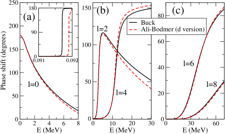
Figure 1: (Color online) Phase shifts (in degrees) as a function of the $\alpha-\alpha$ relative energy obtained with the Buck potential (solid curves) and the d-version of the Ali-Bodmer potential (dashed curves). The results for $\ell=0$ (panel a), $\ell=2,4$ (panel b), and $\ell=6,8$ (panel c) are shown. The inset in panel a shows the phase shifts in vicinity of the 0⁺ resonance in ⁸Be.

The bosonic nature of the $\alpha$-particle constrains the possible excited states to have even angular momenta and positive parity. In Fig.1 we show the phase shifts as a function of the $\alpha-\alpha$ relative energy for the $\ell=0,2,4,6,8$ partial waves. The solid and dashed curves correspond to the results obtained with the Buck potential and the Ali-Bodmer potential, respectively. The inset in panel (a) gives the extremely rapidly varying $s$-wave phase shifts in the vicinity of the $0^{+}$ resonance energy in ⁸Be. The computed phase shifts are remarkably similar for both potentials, even for large relative angular momenta. The computed ⁸Be spectrum is then expected not to change very much from one potential to the other.

As already mentioned, the complex scaling method permits an easy evaluation of the resonance energies and widths. The results obtained for ⁸Be are given in Table 1 along with the experimentally known resonance energies and widths til04 . The Buck and Ali-Bodmer potentials both, as expected from the phase shifts, provide very similar spectra. Together with the $0^{+}$, $2^{+}$, and $4^{+}$ states whose energies and widths reproduce rather well the experimental values, both potentials predict a $6^{+}$ and an $8^{+}$ state at about 34 MeV and 52 MeV, respectively. No experimental evidence of these states is known. In any case, the computed widths for these two last resonances are comparable to their energies and therefore they can not be considered as well defined resonances. A similar proportion between width and energy as for the 2⁺ and $4^{+}$ states would for the same energies give widths of about 2.5 times smaller values, that is 13 MeV and 21 MeV for the $6^{+}$ and $8^{+}$ states, respectively.

An important point to take into account is the fact that the energy of the $0^{+}$ resonance is very sensitive to the $\hbar^{2}/m_{\alpha}$-value (with $m_{\alpha}$ being the mass of the alpha-particle) used in the calculation. The experimentally known value is $\hbar^{2}/m_{\alpha}=10.446$ MeV$\cdot$fm². This is used for all the calculations with the Ali-Bodmer potential. However, when the same value is used with the Buck potential buc77 the $0^{+}$ resonance appears at 0.18 MeV, almost a factor of 2 higher than the experimental value. The potential parameters given in buc77 are therefore probably obtained with $\hbar^{2}/m_{\alpha}=10.368$ MeV$\cdot$fm², which places the $0^{+}$ resonance at the correct value. The effects on the $0^{+}$ resonance and the $s$-wave phase shifts are given in table 1 and the solid line in the inset of Fig.1a. The other resonances (with $\ell>0$) are much less sensitive to this change in $\hbar^{2}/m_{\alpha}$. This original value is maintained when the Buck-potential is used in this paper.

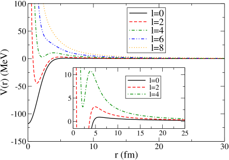
Figure 2: (Color online) Total two-body potential (Buck potential + Coulomb repulsion + Centrifugal barrier) for the lowest angular momenta. The inset shows the details of the potential barrier for $\ell=$ 0, 2, and 4.

The two-body potentials giving rise to all these resonances are shown in Fig.2. Together with the nuclear interaction (that for the figure has been chosen to be the Buck potential) the potentials shown in the figure contain as well the Coulomb repulsion and the centrifugal barrier. For $\ell=0$ the potential barrier is hardly noticeable but the resonance energy is still smaller and the state experiences an extremely thick barrier leading to almost bound state properties. For $\ell=2,4$ the barrier is much higher and thinner but the energy is not far from the top and the resulting widths are rather large. The details of the different potential barriers are shown in the inset. For $\ell=6,8$, the potentials are repulsive. It is therefore surprising that the $S$-matrix poles apparently are well defined and independent of the interactions, determined solely from the phase shifts of the partial waves of smaller $\ell$-values. For this reason we include the results for $\ell=6,8$, although a resonance description is a stretch of this concept.

Table 1: Properties of the five lowest computed resonances in ⁸Be. The first two rows give, when available, the corresponding experimental energies, $E_{r}$, and widths, $\Gamma_{r}$, taken from Ref.til04 . The computed values with the Buck and Ali-Bodmer potentials are given by the third and fourth rows, and by the fifth and sixth rows, respectively. All the energies and widths are given in MeV. The following four rows give, also for the two $\alpha-\alpha$ potentials, the real and imaginary parts of $\sqrt{<r^{2}>}$, computed with the complex scaling method. These values are given in fm. The rows marked $E_{r}^{(0)}$, $E_{r}^{(1)}$, and $E_{r}^{(Z_{0})}$ are rotational energies (in MeV) defined through Eq.(1) and the corresponding moments of inertia $\hbar^{2}/(2{\cal I})$, which are denoted by $B_{0}$ (in MeV) when obtained by fitting the energies through Eq.(1), $B_{1}$ when obtained from Eq.(19) with constant $\alpha$-$\alpha$ distance ($Z_{0}=3.0$ fm), and $B_{Z_{0}}$ when obtained from Eq.(19) with angular momentum dependent $\alpha$-$\alpha$ distance. While $B_{1}$ takes the value of 0.621 MeV, $B_{0}$ and $B_{Z_{0}}$ are angular momentum dependent and they are given in the table for each resonance (the values given for $E_{r}^{(0)}$ have been obtained with $B_{0}=0.475$ MeV, see text). The last row gives the excitation energies obtained in the microscopic cluster model har72 .

$J^{+}$	$0^{+}$	$2^{+}$	$4^{+}$	$6^{+}$	$8^{+}$
$E_{r}$ (Exp.)	0.0918	$2.94\pm 0.01$	$11.35\pm 0.15$	—	—
$\Gamma_{r}$ (Exp.)	$(5.57\pm 0.25)10^{-6}$	$1.51\pm 0.02$	$\sim 3.5$	—	—
$E_{r}$ (Buck)	0.091	2.88	11.78	33.55	51.56
$\Gamma_{r}$ (Buck)	$3.6\cdot 10^{-5}$	1.24	3.57	37.38	92.38
$E_{r}$ (Ali-Bodmer d)	0.092	2.90	11.70	34.38	53.65
$\Gamma_{r}$ (Ali-Bodmer d)	$3.1\cdot 10^{-6}$	1.27	3.07	37.19	93.74
Re$\sqrt{<r^{2}>}$ (Buck)	5.61	3.51	2.93	2.82	2.76
Im$\sqrt{<r^{2}>}$ (Buck)	0.01	1.29	0.82	1.44	1.77
Re$\sqrt{<r^{2}>}$ (Ali-Bodmer d)	5.80	3.58	2.91	2.70	2.73
Im$\sqrt{<r^{2}>}$ (Ali-Bodmer d)	0.001	1.24	0.76	1.40	1.73
$E_{r}^{(0)}=E_{0}+B_{0}J(J+1)$	$E_{0}=0.091$	2.9	9.6	20.0	34.3
$B_{0}$	—	0.475	0.563	0.807	0.721
$E_{r}^{(1)}=E_{0}+B_{1}J(J+1)$	$E_{0}=0.091$	3.8	12.5	26.2	44.8
$E_{r}^{(Z_{0})}=E_{0}+B_{Z_{0}}J(J+1)$	$E_{0}=0.091$	3.2	12.9	28.5	49.1
$B_{Z_{0}}$	—	0.511	0.639	0.677	0.680
$E_{r}$ har72	—	3.8	13.5	30.5	49.7

With the complex rotated wave functions of resonances at hand it is possible to compute the corresponding expectation values of $r^{2}$, which for resonances are complex numbers in contrast to the real values obtained for bound states even if the corresponding wave functions have been complex rotated. As discussed in moi98 , the real part of the expectation value of a given complex rotated operator can be understood as a corresponding average value over continuum wave functions in a range of energies around the resonance. It is then tempting to associate the imaginary part with an uncertainty of the same expectation value. This is analogous to the energy associated with the expectation value of the complex rotated hamiltonian.

In Table 1 the real and imaginary parts of $\langle r^{2}\rangle^{1/2}$ for the five resonances found in ⁸Be with the two different $\alpha-\alpha$ potentials are shown. Again, both potentials give very similar values. We refer to the imaginary parts as the uncertainty which according to gya72 ; moi98 arises from two sources, i.e. the finite width of the state and the fact that the resonance wave function is not an eigenfunction of the $r^{2}$ operator. For the $0^{+}$ case the uncertainty in $\langle r^{2}\rangle^{1/2}$ is very small, as it has to be for such a narrow resonance. For the $2^{+}$ and $4^{+}$ states the uncertainty in the size of the resonance is about three or four times smaller than their average values, while for the $6^{+}$ and $8^{+}$ cases the uncertainty increases up to half the average value. The computed real parts of the average values of $\langle r^{2}\rangle^{1/2}$ are quite similar for the $4^{+}$, $6^{+}$, and $8^{+}$ resonances. By increasing the relative orbital angular momentum, the two $\alpha$-particles appear more and more spatially confined, as discussed below in more details. This apparent confinement is in spite of the broad resonance structures arising from being in the continuum, where extended spatial extension intuitively is expected. It is worth emphasizing that the radii discussed so far are well defined theoretical quantities but they are not observables. The expectation value of the operator $r^{2}$ in a continuum wave function is infinitely large.

The three lowest resonance energies have traditionally been interpreted as energies of a rotational band following the behavior in Eq.(1) with a structure of two $\alpha$-clusters at a given distance from each other. Therefore, the value of $B_{0}=\hbar^{2}/(2{\cal I})$ should be constant, and it could be extracted for instance from Eq.(1) and the energy of the $2^{+}$ resonance. This gives a value of $B_{0}=0.475$ MeV, and the resulting energies of the different levels in the rotational band become those denoted by $E_{r}^{(0)}$ in table 1. In this case the energy of the $4^{+}$ resonance appears at about 2 MeV below the measured (and computed) value, and the energies of the $6^{+}$ and $8^{+}$ states are clearly smaller than the computed ones. Obviously, the reason is that the $B_{0}$ value changes quite a lot when extracted by use of the different resonance energies, as we can see in table 1. The fact that $B_{0}$ is clearly energy dependent suggests that the structure of ⁸Be does not really correspond to a rigid rotor system, i.e., it does not match with an almost frozen deformed structure.

In any case, if we still assume that the two $\alpha$-particles are fixed at positions $z=\pm Z_{0}/2$ on the $z$-axis, the rigid moment of inertia ${\cal I}_{rig}$ around the $y$-axis is then given by:

$${\cal I}_{rig}=\frac{1}{2}m_{\alpha}Z_{0}^{2}+\frac{4}{5}m_{\alpha}R_{\alpha}^{2},$$ (19)

where $m_{\alpha}$ is the mass of the alpha particle, $\langle r_{\alpha}^{2}\rangle^{1/2}\approx 1.7$ fm is its root mean square radius, and the corresponding sharp cut-off radius is $R_{\alpha}^{2}=5/3\langle r_{\alpha}^{2}\rangle$. If we take a $Z_{0}$ value of 3.0 fm we then get $B_{1}=\hbar^{2}/(2{\cal I}_{rig})=0.621$ MeV, which is a kind of average of the four $B_{0}$ values previously obtained. The estimates of the resonance energies from Eqs.(1) and (19) are given in Table 1 as $E_{r}^{(1)}$. The agreement of this rotational sequence with the experimental and computed values is not perfect but perhaps acceptable.

The fact that the intrinsic structure of ⁸Be is changing with angular momentum is also evident from the root mean square radii of the resonances. In other words, the moment of inertia is also angular momentum dependent, and it can be obtained for each resonance from Eq.(19) by simply assuming that for each of them the two $\alpha$-particles are located at the corresponding distances, $Z_{0}=\mbox{Re}\sqrt{\langle r^{2}\rangle}$. In this way, we get the $\hbar^{2}/(2{\cal I}_{rig})$ values given in table 1 as $B_{Z_{0}}$, and the energy sequence, Eq.(1), given by $E_{r}^{(Z_{0})}$. They match very nicely with the energies obtained directly by solving the two-body problem with the corresponding $\alpha-\alpha$ potential. The results for the excitation energies from a classical microscopic cluster model har72 are given in the last row of the table, and they are remarkably similar although obtained with a completely different two-body nucleon-nucleon potential.

This latter result seems to confirm that the ⁸Be spectrum has a rotational character. However, the best agreement has been obtained by using different values of $\mbox{Re}\sqrt{\langle r^{2}\rangle}$ for $Z_{0}$ for each resonance. The moments of inertia are correspondingly very different, and surprisingly the largest variation in $\sqrt{\langle r^{2}\rangle}$ is found for the lowest two, 0⁺ and 2⁺, of the three experimentally known states. This fact reveals that the idea of ⁸Be as a rigid rotor of two alpha particles separated by a given distance is questionable. Only for the 4⁺, $6^{+}$, and $8^{+}$ states the distance remains roughly the same, and therefore also ${\cal I}_{rig}$ is more stable. However, it is worth emphasizing that the intrinsic $\alpha$-particle structure still is maintained, although the particles are located at different separation.

III.2 Transitions

In Section II.2 we have described two different methods to obtain the transition strength ${\cal B}^{(E2)}$ from the computed cross section for a given transition. The first one assumes a Breit-Wigner shape for the cross section in the vicinity of the resonance energy for the incident channel. This fact permits to extract the decay probability $\Gamma_{\gamma}$ for that transition and, from Eq.(17), obtain then the transition strength. We shall denote the strength computed in this way as ${\cal B}^{(E2)}_{\gamma}$.

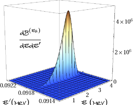
Figure 3: (Color online) Contour plots of the transition strength in Eq.(8) as function of initial, $E$, and final state, $E^{\prime}$, energies. The units are $e^{2}$ fm${}^{4}/$MeV². The Buck potential is used. Upper and lower parts are for $2^{+}\rightarrow 0^{+}$ and $4^{+}\rightarrow 2^{+}$, respectively.

The second method constructs $d{\cal B}^{(E2)}/dEdE^{\prime}$ by dividing the differential cross section in Eq.(7) by the average value of the photon energy and by the remaining constant factors. Integration of the differential transition strength around the peak of the resonance provides the total transition strength that will be denoted as ${\cal B}^{(E2)}_{\sigma}$. In Fig.3 we show the $d{\cal B}^{(E2)}/dEdE^{\prime}$ strength for the $2^{+}\rightarrow 0^{+}$ and $4^{+}\rightarrow 2^{+}$ transitions. The distribution for the first case is a very thin slice of the given final state energy along the initial energy, both directions extending roughly as far as the respective resonance widths. This is for the same reason reflected in the contour plot of the much broader $4^{+}\rightarrow 2^{+}$ transition.

The transition strengths obtained with these two methods depend on the energy window chosen around the resonance energy in the final state. This window defines the integration range for $E^{\prime}$ in Eq.(5). In Ref.gar13 the details about these two methods are given, as well as the transition-strength values obtained with them for different final energy windows. We have also found that the computed strengths are insensitive to the two-body potential used, and, for this reason, from now on only the results obtained with the Buck potential will be given.

In table 2 we have collected the results obtained in gar13 for the $2^{+}\rightarrow 0^{+}$, $4^{+}\rightarrow 2^{+}$, $6^{+}\rightarrow 4^{+}$, and $8^{+}\rightarrow 6^{+}$ transitions for final energies $E^{\prime}$ within the windows $E^{\prime}_{r}\pm\Gamma^{\prime}_{r}/2$ and $E^{\prime}_{r}\pm\Gamma^{\prime}_{r}$, where $E^{\prime}_{r}$ is the resonance energy in the final channel and $\Gamma^{\prime}_{r}$ its corresponding width. These results are in fairly good agreement with the ones obtained in lan86 ; lan86b (8^th column in the table). However, the strength obtained for the $2^{+}\rightarrow 0^{+}$ transition in Quantum Monte-Carlo calculations wir00 is clearly smaller, although similar to gar13 ; lan86 ; lan86b for the $4^{+}\rightarrow 2^{+}$ case (9^th column in the table). The results shown for the $4^{+}\rightarrow 2^{+}$, transition are consistent with the experimental value of $25\pm 8$ $e^{2}$fm⁴ quoted in dat05 .

Table 2: ${\cal B}^{(E2)}$-values (in $e^{2}$fm⁴) for the different possible $E2$-transitions between the ⁸Be resonances. Columns from two to five are the results obtained in gar13 with the two methods described in the text for a final energy window $E^{\prime}_{r}\pm\Gamma^{\prime}_{r}/2$ (2^nd and 3^rd columns) and $E^{\prime}_{r}\pm\Gamma^{\prime}_{r}$ (4^th and 5^th columns), where $E^{\prime}_{r}$ and $\Gamma^{\prime}_{r}$ are the energy and width of the resonance in the final state. The next two columns are the results obtained assuming a rotational model, Eq.(20), when $Z_{0}$ is fixed to 3 fm (6^th column) and when $Z_{0}$ is taken equal to $\mbox{Re}\sqrt{\langle r^{2}\rangle}$ for each resonance (7^th column). The results within parenthesis are the ratios ${\cal B}^{(E2)}(\ell\rightarrow\ell^{\prime})/{\cal B}^{(E2)}(2^{+}\rightarrow 0^{+})$ for each of the calculations. The results from previous calculations wir00 ; lan86 ; lan86b ; har72 are given in columns 8 to 10. The last column is the result obtained after a complex scaling calculation assuming a resonance to resonance transition.

${\cal B}^{(E2)}$	$E^{\prime}_{r}\pm\Gamma^{\prime}_{r}/2$		$E^{\prime}_{r}\pm\Gamma^{\prime}_{r}$		Rotational model		lan86 ; lan86b	wir00	har72	Comp. scaling.
	${\cal B}^{(E2)}_{\gamma}$	${\cal B}^{(E2)}_{\sigma}$	${\cal B}^{(E2)}_{\gamma}$	${\cal B}^{(E2)}_{\sigma}$	$Z_{0}=3$ fm	$Z_{0}$
$2^{+}\rightarrow 0^{+}$	53.4 (1)	32.9 (1)	79.1 (1)	48.4 (1)	6.4 (1)	84.0 (1)	71.3	14.8	16.8	$-4.6+i33.6(1)$
$4^{+}\rightarrow 2^{+}$	15.5 (0.29)	12.1 (0.37)	22.1 (0.28)	17.2 (0.36)	9.2 (1.43)	18.1 (0.22)	18.0	18.2	25.9	$2.1+i11.8(0.336-i0.0483)$
$6^{+}\rightarrow 4^{+}$	6.7 (0.13)	4.5 (0.14)	10.1 (0.13)	6.9 (0.14)	10.1 (1.57)	9.1 (0.11)	-	-	33.9	$3.0+i12.6(0.356-i0.139)$
$8^{+}\rightarrow 6^{+}$	6.6 (0.12)	2.5 (0.08)	13.0 (0.16)	5.2 (0.11)	10.6 (1.65)	7.6 (0.09)	-	-	-	$-6.1+i13.2(0.410+i0.124)$

An additional, and in a sense decisive, test of the rotational character of the states in ⁸Be is provided by the total transition strength given in Eq.(16). For rotational bands with an inert intrinsic structure, the total strength for two inert $\alpha$-particles at $\pm Z_{0}/2$ is bohrII

$${\cal B}^{(E2)}(\ell\rightarrow\ell^{\prime})=\frac{5e^{2}}{4\pi}Z_{0}^{4}\langle\ell 020|\ell^{\prime}0\rangle^{2}\;.$$ (20)

The spatial extension of the spherical $\alpha$-particle distribution does not enter this expression in contrast to the moment of inertia in Eq.(19). The different transition strengths are then related by the expression:

$$\frac{{\cal B}^{(E2)}(\ell_{i}\rightarrow\ell^{\prime}_{f})}{{\cal B}^{(E2)}(\tilde{\ell}_{i}\rightarrow\tilde{\ell^{\prime}}_{f})}=\frac{\langle\ell_{i}020|\ell^{\prime}_{f}0\rangle^{2}}{\langle\tilde{\ell}_{i}020|\tilde{\ell^{\prime}}_{f}0\rangle^{2}}\;.$$ (21)

The approximation in Eq.(21) is valid for rigorous rotational bands, and therefore in particular also for two rotating $\alpha$-particles where Eq.(20) applies. Comparing to Eq.(16) this is seen to imply that the integrals should be independent of the transition, which reflects that the radial wave functions and then the intrinsic structure is the same for all the states.

In the schematic rotational model of Eq.(20) we get all the transition strengths for a given $Z_{0}$. They are useful for comparison and interpretation. We first choose a constant $Z_{0}=3$ fm, which was the value chosen to obtain the sequence of states denoted by $E_{r}^{(1)}$ in table 1. The strength values given by Eq.(20) are shown in the 6^th column of table 2. They are clearly different to the ${\cal B}^{(E2)}$-values obtained in gar13 , no matter the size of the window used and the procedure used to extract it. It is quite clear that the transition strengths do not follow the rule dictated by the strict rotational model.

The same conclusion is reached when examining the transition strength ratios. The value of $\langle\ell_{i}020|\ell^{\prime}_{f}0\rangle^{2}$ is 0.2, 0.29, 0.31, and 0.33 for the $2^{+}\rightarrow 0^{+}$, $4^{+}\rightarrow 2^{+}$, $6^{+}\rightarrow 4^{+}$, and $8^{+}\rightarrow 6^{+}$ transitions, respectively. When taking the $2^{+}\rightarrow 0^{+}$ transition as a reference, the ratios given by the rotational model, Eq.(21), are shown by the numbers within parenthesis in the 6^th column of the table. The last three transitions should then have a rather similar strength, which in turn should be larger than the strength corresponding to the $2^{+}\rightarrow 0^{+}$. Nothing of this happens with the $\alpha-\alpha$ potentials. The ratios obtained with the transition strengths in Ref.gar13 (given by the corresponding numbers within parenthesis in each of the columns in table 2) are clearly smaller, and the maximum transition strength is actually obtained for the $2^{+}\rightarrow 0^{+}$ transition.

The behavior predicted by the rotational model coincides with the one found with the microscopic cluster model har72 (10^th column in the table), although the absolute values are about a factor of 3 different. This corresponds to a larger value of $Z_{0}\approx 4$ fm consistent with the spatial extension found in har72 . This resemblance of the rotational model and the classical microscopic cluster model results is perhaps not very surprising, since the $\alpha-\alpha$ structure after all is imposed in both cases.

However, the cluster model in har72 is based on a generator coordinate description where angular momentum projection before and after variation both start out with the same $\alpha-\alpha$ cluster structure. The different angular momentum states are then related through a similar intrinsic structure, which can be somewhat differently deformed depending on angular momentum, but still the basic rotational model assumptions are approached and almost fulfilled. In contrast, the potential models with effective $\alpha-\alpha$-interactions provide independent solutions for each of the angular momenta. The solutions are only related through the same central potential.

It is then clear that the radial integrals in Eq.(16) change with angular momentum and produce unexpected transition strengths. The different spatial structure of the resonances was already seen when analyzing the $\langle r^{2}\rangle^{1/2}$-values, which for instance for the $0^{+}$ case is about twice the value in the $4^{+}$, $6^{+}$, or $8^{+}$ cases. In fact, in the previous section we saw that when using different values for $Z_{0}=\mbox{Re}\sqrt{\langle r^{2}\rangle}$ for each resonance, the energy sequence in ⁸Be was nicely reproduced. It is then very tempting to check if the same good agreement is recovered when using $Z_{0}=\mbox{Re}\sqrt{\langle r^{2}\rangle}$ for each resonance in Eq.(20). More precisely we have chosen for each transition the $Z_{0}$ value corresponding to the final state resonance. The results obtained are given in the 7^th column of table 2. As we can see, now the agreement with the results in gar13 is definitely much better, especially with the ${\cal B}^{(E2)}_{\gamma}$-values when using the $E^{\prime}_{r}\pm\Gamma^{\prime}_{r}$ final energy window. As a consequence, the corresponding ratios (numbers within parenthesis) also agree much better now. This result seems to confirm the conclusion reached in the previous section, namely, the ⁸Be spectrum has a rotational character provided that the $\alpha-\alpha$ distance is angular momentum dependent. Still the principal $\alpha$-cluster structure is maintained.

IV Discussion

To discuss quantitatively we should preferentially apply the method to specific systems as we did in the previous sections. We shall here first discuss the radial dependence of wave functions in the continuum. This is numerically simple by use of the complex scaling method. However, the properties of the corresponding complex rotated wave function then only represent a part of the cross section. Other parts related to continuum contributions are necessary to obtain the full observable cross sections. Complex scaling mixes these contributions in a complicated manner, but we expect the resonance structures to be strongly indicative for the overall behavior.

To supplement we discuss instead the properties of the wave functions and the resulting transitions for real energies, where the interesting physics is hiding behind diverging integrals. We continue to discuss basic conditions for appearance of rotational motion in two-body systems. We then turn high-spin states created in heavy-ion collisions often claimed to be of rotational structure.

IV.1 Continuum resonance structures

The definition of transition probabilities is in practice not well defined since the states are not well defined either in the continuum. It is then interesting to know the results for transitions between the rigorously defined resonance states found by complex rotation. However, the probabilities are then “rotated” into the complex values given in the last row of table 2. The results in the present work do not depend significantly on the potential, and we therefore only give the results for the Buck potential. They are independent of rotation angle as required by well defined resonances, but obviously they cannot represent observable quantities. First, the results are complex numbers. Second, they are only part of the full observables, which include both resonance-to-resonance and continuum background contributions gar13a ; myo98 .

The ratios of these partial transition probabilities (in brackets in the last column in table 2) now show the same behavior of the factor of $3$ decrease from the $2^{+}\rightarrow 0^{+}$ to the $4^{+}\rightarrow 2^{+}$ transition as for the full calculation using only real energies. The imaginary part is 10 times smaller than the real part. However, the real parts of the next two ratios involving the rather artificial $6^{+}$ and $8^{+}$ resonances increases almost in line with the schematic rotational model. The imaginary parts of these complex numbers are still a factor of 3 smaller than the real parts of these ratios.

Therefore, the observable relative transition probabilities for the first 3 resonances (not the last) in the first columns of table 2 are almost recovered in the complex resonance-to-resonance relative transitions. These can in turn be understood by their decreasing $\sqrt{\langle r^{2}\rangle}$-values of the resonances as given in table 1. Thus, we can conclude that the very large deviations from the rotational model arise from a decreasing spatial extension of the $0^{+}$, $2^{+}$ and $4^{+}$ resonances.

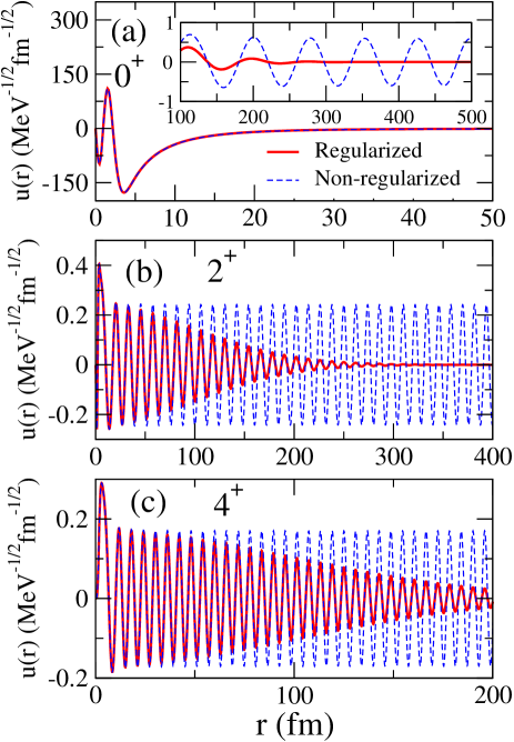
Figure 4: (Color online) The radial wave functions for the three lowest resonances, $0^{+}$, $2^{+}$, and $4^{+}$, are shown as function of $r$. The solid and dashed curves correspond to the regularized and non-regularized wave functions, respectively. The regularization has been performed by introducing the Zel’dovich factor $\exp(-\eta^{2}r^{2}/2)$, with $\eta=0.01$ fm^-1. The energy of each wave function is taken at the center of the resonance, $E_{r}$.

However, an understanding of the properties obtained entirely by calculations for real energies is much more complicated. Nevertheless, we shall in the following attempt a detailed explanation. The radial wave functions for the lowest three resonances are shown in Fig.4 both non-regularized and multiplied by an appropriate Zel’dovich factor. In principle, for a given value of the Zel’dovich parameter, the radial wave functions should be accordingly renormalized, such that Eqs.(4) or (10) are restored. However, the wave functions are already initially normalized, and when taking the limit of zero $\eta$-value the correct normalization condition is recovered faster than the converged value of the radial integral. Therefore, in practice the renormalization is not needed.

As seen in the figure, the $0^{+}$ state behaves as a bound state, although tiny oscillations are visible at large distances before the Zel’dovich cut-off becomes efficient (inset in Fig.4a). The two nodes at small distances are due to the deep potential with two spurious strongly bound states.

For both the $2^{+}$ and $4^{+}$ resonances the oscillations are very pronounced up to about $200$ fm, where the Zel’dovich regularized wave function essentially has vanished. The resonance structures are only visible at very small distances, where the first oscillation of each state inside the attractive region of the potential, has twice the amplitude of the second. Note that in Fig.4 only the radial wave functions $u(r)$ are shown, while the total radial wave function is actually given by $u(r)/r$. When dividing by $r$ we can see that the $0^{+}$ resonance behaves as a bound state, and both, the $2^{+}$ and $4^{+}$ states, reveal resonance character only at distances smaller than about $5$ fm. The period in the oscillations in Fig.4 depends only on the resonance energies through the wave number, $k=\sqrt{2\mu E/\hbar^{2}}$, which gives wave lengths $2\pi/k\approx 70$ fm, 12 fm, and 6 fm, respectively. The Coulomb barriers for these states extend correspondingly to about 60 fm, 10 fm, and 5 fm, that is the regular oscillations all occur outside the barriers for positive kinetic energies.

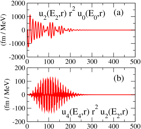
Figure 5: (Color online) The radial integrands of the two lowest transitions, $2^{+}\rightarrow 0^{+}$ and $4^{+}\rightarrow 2^{+}$ as function of $r$ after Zel’dovich regularization with the factor (squared) in Fig.4, and for the same energies.

The transitions are determined as integrals over radial wave functions, see Eq.(16). We show in Fig.5 the integrands of the matrix elements for the lowest transitions for energies corresponding to resonance peaks. The oscillations appearing now are the results of combining the two oscillating wave functions. Their different periods produce the different (from the wave functions) but regular oscillation extending to about 200 fm. For $2^{+}\rightarrow 0^{+}$, the revival after destructive interference is seen before the Zel’dovich cut-off reduce the amplitude to be insignificant. For $4^{+}\rightarrow 2^{+}$, the amplitude increases to about 100 fm/MeV up to 100 fm and is in fact only a few fm/MeV at small distances.

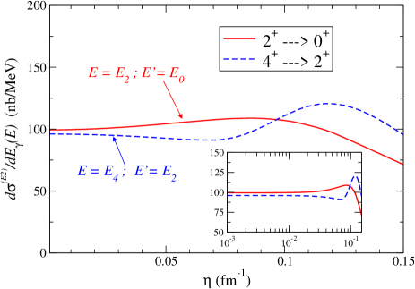
Figure 6: (Color online) Differential cross section (Eq.(2)) for given initial and final energies ($E$ and $E^{\prime}$) for the $2^{+}\rightarrow 0^{+}$ (solid curve) and $4^{+}\rightarrow 2^{+}$ (dashed curve) transitions in ⁸Be as a function of the Zel’dovich parameter $\eta$. The initial and final energies for each transition correspond to the $0^{+}$, $2^{+}$, and $4^{+}$ resonance energies (same energies as in Figs.4 and 5). The inset shows the same as in the main figure but with the $\eta$-axis in logarithmic scale.

It is now highly significant that the integrals themselves are only a few fm²/MeV. This means that the oscillations of the integrands cancel to a very large extent, where it may be necessary to emphasize that a substantial range of Zel’dovich parameters, $\eta\lesssim 0.1$ fm^-1, produces precisely the same matrix element. This is illustrated in Fig.6, where the solid and dashed curves show the integrals of the functions in Figs.5a and 5b, but as a function of the Zel’dovich parameter $\eta$. As we can see, for sufficiently small values of $\eta$, the computed integrals become constant. The wave functions and the matrix elements in Figs.4 and 5 are shown for $\eta=0.01$ fm^-1, which reveal the large amplitude oscillations at rather large distances. A variation of $\eta$ from very small to large values, $\eta\sim 0.01$ fm^-1, would move the damping of the wave functions in Fig.4 and the oscillating structures in Fig.5 down to smaller distances, bit still leaving untouched the small distance part of the wave functions, where the resonance structure is contained.

It is then remarkable that the transition probabilities between states of given energies are numerically well defined to values much smaller than corresponding to the large amplitudes at large distances. However, to extract the decisive short-distance properties of the resonance wave functions is much more difficult. The cancellation at large distances implies that these oscillations only play a minor role in the determination of the transition probability. In fact, only distances of less than about $5$ fm contribute corresponding to the spatial extension of the regions where resonance character is seen in Fig.4. To be on the safe side where the matrix elements still can be reliably obtained numerically, we choose the value of $\eta=0.01$ fm${-1}$ in all cases investigated in the present work. More detail will be presented in ref.gar13a .

If we use the complex scaling method, the oscillations in Figs.4 and 5 disappear altogether in the complex scaled resonance wave functions, and radii and transition matrix elements are well defined. This does not prevent larger distances from giving significant contributions. The smaller radii for larger angular momenta seen in table 1 are the opposite of the ordinary centrifugal stretching. This is related to properties of real energy calculations where the increasing widths of the resonances arise as they approach the top of the barriers. The states then approach free waves in most space.

The free wave oscillations are quickly approached in Figs.4 and 5 before the Zel’dovich factor is applied. Only deviations from the free wave can contribute to resonance properties, and in turn to results for transition probabilities like ${\cal B}^{(E2)}$-values. Therefore, the smaller the radii of the space exhibiting deviations from free waves, the smaller are the radial moments, and in turn the radial transition matrix elements also decrease.

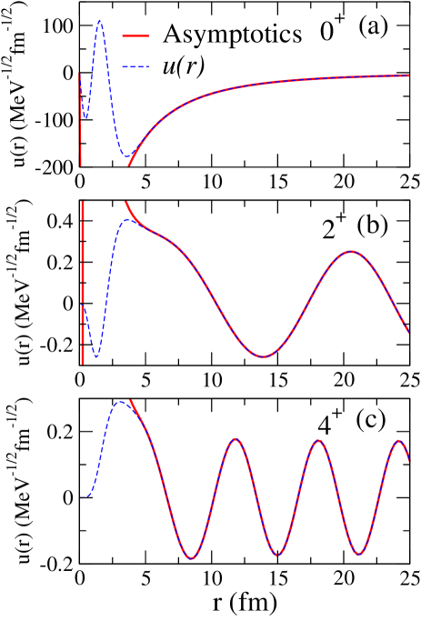
Figure 7: (Color online) The solid curves show the asymptotic wave function, Eq.(3), for the three lowest resonances, $0^{+}$, $2^{+}$, and $4^{+}$. The corresponding radial functions $u(r)$, already shown in Fig.4, are given by the dashed curves. The energy of each wave function is taken at the center of the resonance, $E_{r}$.

To understand this a little better we turn to the asymptotic behavior of the continuum wave functions in Eq.(3). Let us first define the asymptotically vanishing function

$$\tilde{u}_{\ell}(E,r)=u_{\ell}(E,r)-u_{\ell}^{asymp}(E,r)\;$$ (22)

$$u_{\ell}^{asymp}(E,r)=\lim_{r\rightarrow\infty}u_{\ell}(E,r)\;.$$ (23)

The remaining function, $\tilde{u}_{\ell}$, now contains the resonance structure revealed at short distances, and traces of the oscillating continuum structures are removed. The precise asymptotic behavior from Eq.(3) is only correct for point-like charge distributions, or at distances where the charges do not overlap. At smaller distances the function in Eq.(3) is incorrect and even diverging for distances approaching zero. To get physically meaningful results we have to account for the finite extension of the charges. This is easily done by a regularization procedure or by extending the Coulomb wave functions down to zero by combinations of sine and cosine functions as in the case of no Coulomb interaction or from the corresponding asymptotic limit of the Coulomb functions. We choose first the true asymptotics from Eq.(3) and show in Fig.7 the three resonance wave functions, $u$ (dashed curves), and its asymptotic behavior (solid curves), as function of $r$. At distances larger than $5$ fm the full and the asymptotic wave functions are indistinguishable. This is in full agreement with the resonance radii in Table 1, Fig.4, as well as the discussion in connection with the transition matrix elements in Fig.5.

The division into short and asymptotic parts in Eqs.(22) and (23) is now directly applicable in a separation of contributions from the different parts. This is highly desirable in analyses of experimental data using the $R$-matrix formulation where any continuum contribution appears as spurious resonances strongly depending on the channel radius. We can calculate the radial transition matrix element, $B_{\ell,\ell^{\prime}}(E,E^{\prime})=\langle u_{\ell}(E,r)|r^{2}|u_{\ell^{\prime}}(E^{\prime},r)\rangle$, which naturally is divided into four types of terms involving short-distance and asymptotic parts in different combinations, i.e.

$$B^{(sh,sh)}_{\ell,\ell^{\prime}}=\langle\tilde{u}_{\ell}(E,r)|r^{2}|\tilde{u}_{\ell^{\prime}}(E^{\prime},r)\rangle\;,$$ (24)

$$B^{(sh,as)}_{\ell,\ell^{\prime}}=\langle\tilde{u}_{\ell}(E,r)|r^{2}|{u}^{asymp}_{\ell^{\prime}}(E^{\prime},r)\rangle\;,$$ (25)

$$B^{(as,sh)}_{\ell,\ell^{\prime}}=\langle{u}^{asymp}_{\ell}(E,r)|r^{2}|\tilde{u}_{\ell^{\prime}}(E^{\prime},r)\rangle\;,$$ (26)

$$B^{(as,as)}_{\ell,\ell^{\prime}}=\langle{u}^{asymp}_{\ell}(E,r)|r^{2}|{u}^{asymp}_{\ell^{\prime}}(E^{\prime},r)\rangle\;,$$ (27)

$$B_{\ell,\ell^{\prime}}=B^{(sh,sh)}_{\ell,\ell^{\prime}}+B^{(sh,as)}_{\ell,\ell^{\prime}}+B^{(as,sh)}_{\ell,\ell^{\prime}}+B^{(as,as)}_{\ell,\ell^{\prime}}\;,$$ (28)

where the notation of the contributions to $B_{\ell,\ell^{\prime}}$ refers to short-distance and asymptotic combinations. A tempting interpretation is the correspondence of contributions from respectively resonance to resonance $(sh,sh)$, resonance to continuum $(sh,as)$, continuum to resonance $(as,sh)$, and continuum to continuum $(as,as)$.

At very large distances the wave functions $u_{\ell}$ are governed by a combination of sine and cosine functions of $(\kappa r)$, as it can be seen from Eq.(3). The terms of the type $B^{(as,as)}_{\ell,\ell^{\prime}}$ contain then in the integrand products of either two sine functions, or two cosine functions, or one sine and one cosine functions. These integrals are therefore not well defined unless the Zel’dovich regularization is applied. When done, we obtain vanishing results both when two $\sin(\kappa r)$-type and two $\cos(\kappa r)$-type functions are combined, whereas finite results emerge when products of $\sin(\kappa r)$ and $\cos(\kappa^{\prime}r)$ functions appear (or the other way around). These conclusions assume that $E\neq E^{\prime}$. All other terms in $B_{\ell,\ell^{\prime}}$ have the $\tilde{u}$-functions as factors, and the corresponding integrals are convergent and well defined.

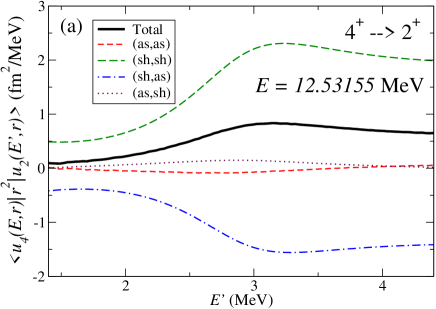
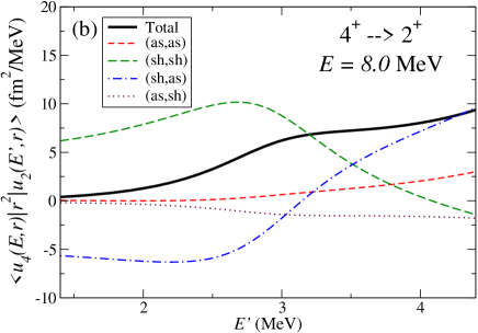
Figure 8: (Color online) Radial transition matrix element $B_{\ell,\ell^{\prime}}(E,E^{\prime})$ for the $4^{+}\rightarrow 2^{+}$ transition as a function of the final energy $E^{\prime}$. The total transition matrix element is given by the solid curve. The $(as,as)$, $(sh,sh)$, $(sh,as)$, and $(as,sh)$ contributions are shown by the short-dashed, long-dashed, dot-dashed, and dotted curves, respectively. In part (a) the initial energy is $E=12.53155$ MeV for which the $4^{+}$ phase-shift is equal to $\pi/2$. In part (b) the initial energy ($E=8$ MeV) has been chosen to be outside the $4^{+}$ resonance peak.

One immediate consequence is that $B^{(as,as)}_{\ell,\ell^{\prime}}$ is zero when initial and final state wave functions both correspond precisely with resonance states, where the phase shifts are $\pi/2$. The products of the asymptotic parts are equal to zero since $\cos(\pi/2)=0$, and only terms of the type $\cos(\kappa r)$ survive in the asymptotic part of the wave function. Therefore, only terms where the $\tilde{u}$ wave functions enter give non-vanishing contributions to $B_{\ell\ell^{\prime}}$. This is illustrated in Fig.8a, where we plot $B_{4^{+},2^{+}}(E,E^{\prime})$ as a function of the final energy $E^{\prime}$ and for an initial energy of $E=12.53155$ MeV, which corresponds to a $4^{+}$ phase-shift equal to $\pi/2$. The total value is shown by the solid curve. The $B^{(as,as)}_{4^{+},2^{+}}$-contribution is given by the short-dashed curve, which is very small for all the final energies shown, and it is particularly close to zero in the vicinity of $E^{\prime}=3.33$ MeV, which is the value at which the 2⁺ phase shift is $\pi/2$.

This is consistent with our classical intuition where resonances are located in the continuum with large amplitudes at short distances and comparably small and non-contributing amplitudes at large distance. Still, even here the terms $B^{(as,sh)}_{\ell,\ell^{\prime}}$ and $B^{(sh,as)}_{\ell,\ell^{\prime}}$ are non-vanishing, although only relatively short distances can contribute due to the $\tilde{u}$-functions. These terms may represent unavoidable continuum background contributions as it can be seen in Fig.8a, where especially the $(sh,as)$ contribution (dot-dashed curve) is very significant. The interference between the different contributions is very substantial. However, the contributions must arise from radii where the $\tilde{u}$ functions are finite, that is the large amplitude oscillation seen in Fig.5 necessarily cancels completely.

When the initial and final state energies differ from the resonance energies the $B^{(as,as)}_{\ell,\ell^{\prime}}$-contribution is then not identically equal to zero, although well defined after the Zel’dovich regularization. This is shown in Fig.8b, where the initial energy ($E=8$ MeV) does not correspond to any $4^{+}$ resonance. The interference contribution is again substantial. In this case the $(as,as)$ contribution (short-dashed curve) is clearly relevant, although the major contribution from the asymptotic part is again the $(sh,as)$ one, given by the dot-dashed curve.

We are now equipped to summarize the validity of the ordinarily used long wavelength approximation where the contributing radii should be smaller than the inverse of the wave number. The total resonance wave function in Fig.4 reveals a larger amplitude at small distances than for the asymptotic oscillations. This is much clearer seen in Fig.7, where the deviation between full and asymptotic wave functions are shown. The radial extension is in agreement with the root-mean-square values of the resonances given in Table 1. The contribution to the matrix elements arise from rather small distances as seen by comparing amplitudes of the integrand in Fig.5 with the very much smaller integrated result. The large large-distance oscillations must therefore essentially cancel.

The non-vanishing values of $\tilde{u}$ necessary to get contributions are confined to radii less than 5 fm as seen in Fig.7. This is much smaller than the smallest contributing wavelength of $25$ fm arising from the largest contributing photon energy of $10-12$ MeV. The estimate of the contributing photon energy interval can be seen in Fig.3, where we show the distribution of strength for the transition cross sections from given initial to final state energies. The bulk contribution are concentrated in peaks corresponding to a photon energy of substantially less than $12$ MeV in the worst case of the tail of the $4^{+}\rightarrow 2^{+}$ transition. Thus, the long wavelength approximation is rather accurate.

IV.2 Validity of the rotational model

The classical rotation of an isolated inert system is characterized by its kinetic energy, which can be expressed as either the square of the angular momentum divided by twice the moment of inertia around the rotation axis, or half of the square of the rotation frequency times the same moment of inertia.

The convenient quantum mechanical version is in terms of the conserved and quantized angular momentum. An ideal analogue is then a two-body cluster structure with a strongly attractive one-dimensional delta-shell potential like $\delta(r-Z_{0})$. The ground state wave function of zero angular momentum is localized at the relative distance $r=Z_{0}$. This corresponds to an intrinsic wave function localized in one point, $z=Z_{0}$, and averaged with equal weights over all spatial directions. For finite angular momentum, $\ell$, the energy is increased by $\hbar^{2}\ell(\ell+1)/(2{\cal I})$, where ${\cal I}=\mu Z_{0}^{2}$. The relative distance for a bound state would still be $Z_{0}$, and the use of relative coordinate requires the use of the reduced mass $\mu$. The rotational spectrum is then recovered.

For an attractive potential of finite range like a square well or a gaussian potential, the rotational structures do not automatically appear. A repulsion at short distance and a confining barrier at larger distances would lead to a potential of $\delta$-shell character. If it is deep enough the rotational spectrum would then again arise. These repulsive potentials could in principle be provided by a Coulomb interaction between point-like particles. Both short and long-range repulsions would appear. However, these barriers are very easily either small or not present at all.

Conditions for a rotational spectrum with only an attractive finite range potential can be seen by use of simple potentials. The harmonic oscillator potential gives energies linear in $\ell$ while the energies for a spherical square well potential are more promising. For a deep-lying bound state the boundary condition is approximately, $j_{\ell}(\kappa R)=0$, where $j_{\ell}$ is the spherical Bessel function of order $\ell$, $R$ is the radius and $\kappa$ the wave number. The nodes of these Bessel functions approach $(\ell+1/2)(1+1.86/(\ell+1/2)^{2/3})$ for large $\ell$, and the corresponding energies found from the square of $\kappa$ are then approaching $(\ell+1/2)^{2}$ which is the semiclassical analog of $\ell(\ell+1)$. Thus in this limit the rotational spectrum also emerges, and three levels of the rotational sequence can approximately be reproduced with one free parameter like the radius or the moment of inertia. Then, we conclude that if a flat potential is sufficiently deep then the rotational energy sequence arises. This reflects the classical knowledge that the kinetic energy is responsible for the rotational character of a system described by a rotational invariant hamiltonian. The other limit, where the potential is unable to support bound states of non-zero or moderate angular momenta, is for the same reason not necessarily of rotational character. It is then somewhat surprising that the ⁸Be states to some extent reveal this character even as resonances.

For states deeply bound in a short-range attractive potential the centrifugal barrier term is comparatively small and the radial wave functions are expected to be roughly independent of $\ell$. Then the rotational sequence of transition probabilities would be approximately obeyed. However, these states must be strongly bound, and certainly not simply unbound resonance structures in the continuum. We can then conjecture that the rotational model for a two-body inert structure is valid for very strong short-range attractions, and viceversa invalid when the attraction becomes comparable to the centrifugal barrier term.

It is still not excluded that resonance structures approximately could obey the necessary independence of the radial integrals in order to validate the rotational transition sequences. The regularization of the continuum wave functions influences the corresponding radial integrals but it is not obvious that the higher-lying energy and angular momentum states are less spatially extended. The explanation is that the oscillating behavior appears at shorter distances when the state is closest to the barrier. The regularization removes the corresponding contribution by subtraction of the diverging large-distance part of the wave function. The result is decreasing radial integral and increasing deviation from the rotational model. This could be an artifact of the present procedure but the measured datum confirms this interpretation. It is therefore highly interesting to obtain more experimental data for verification or possibly falsification of the present interpretation.

We should finally emphasize that the presence of other types of excitation also may destroy the validity of the pure rotational model. Such bound states or resonances are abundantly arising from intrinsic degrees of freedom or other collective motion like vibrations. Effective decoupling of rotational states from other excited states would be achieved when the excitation energies of the rotations are much lower than all other excitations. However, this can not continue indefinitely to high excitations where other degrees of freedom may be excited as well. For comparable energies the coupling producing mixed states can be very moderate and the pure pictures are no longer valid. It is still possible to have rotational states at relatively high energy provided that other degrees of freedom either produce excited states far away and of much larger energy separation than the rotations, or in practice decoupled due to e.g. disparate structures of all other excited states of comparable excitation energies.

IV.3 Rotational states of heavy nuclei

The fact that a large number of nuclear spectra exhibit rotational structure bohrII ; cas00 demands an explanation. The heavy-ion populated high-spin states reach more than 50 units of $\hbar$. Many different high-spin bands apparently appear in the same nucleus, a typical example can be found in ril88 . Transitions are measured between intra, as well as inter, band members. Still, the interpretation is in terms of rotational bands.

As discussed above, the validity of the rotational model seems to rely on an effectively strong binding which allows the exited states to be strongly bound as well. This is achieved for nuclear states where lifetimes or widths are determined or dominated by photon emission processes. Any other decays like fission, nucleon and cluster emission are then strongly hindered. A barrier must then effectively be present in all other decay channels than photon emission. The result is that the nucleus then must behave as a strongly bound system.

This apparent strong binding can be directly due to a huge barrier against decay as for example fission of intermediate mass nuclei. A barrier may also be effectively present if restructuring is required to arrive at the final decay product as for example for $\alpha$-emission of nuclei without traces of $\alpha$-clustering.

The pronounced rotational structures are also first of all found for relatively small energies. The numerous high-spin states and the abundantly experimentally obtained rotational spectra are not necessarily contradicting this interpretation.

The transition probabilities for the high-spin states are also often not following the rotational model that well. There is always the centrifugal stretching, higher order corrections even to the rotational energy spectra, deformation and pairing variations, etc. bohrII ; cas00 . Furthermore, if the preferred decay channel is fission, particle or cluster emission, the large width of the states prohibit accurate direct measurement of the transition probabilities. Such states may possibly be members of a rotational sequence of energies, but their photon emission probabilities are not observables. A full population and decay history in terms of cross sections are required to get a meaningful description as in the case of ⁸Be discussed in this paper.

V Summary and conclusion

We investigate the simplest structure able to exhibit quantum mechanical rotational motion: two spin-zero inert $\alpha$-particles. We first sketch the formalism which is precisely valid for bound states, but present increasing problems as the continuum properties becomes more pronounced. We first explain that it is absolutely necessary to use observables for continuum calculations. The structure information via the ${\cal B}^{(E2)}$-values cannot be obtained directly without very severe restrictions to energies around the resonances between which the transition occurs.

Staying with observables has the positive implication that direct comparison with measurements is possible. However, the structure information is then hidden in pieces of the observables. One conclusion is therefore that structure and reaction cannot be disentangled and we have to live with this lack of information about the continuum structures. We show that it is possible to derive structure information, although the results are inherently uncertain due to the unavoidable use of non-observable quantities. We describe two procedures to derive the non-observable ${\cal B}^{(E2)}$-values which contain information about the structure of the resonances.

We show that the rotational energy sequence and corresponding radii are followed by the resonances. However, in contrast the transition probabilities deviate substantially from the rotational model predictions. First, this is not due to the uncertainties arising from the extraction of these non-observable continuum properties. It is also not due to neglect of intrinsic $\alpha$-structure, $\alpha$-polarization or effective charges, or centrifugal stretching effects. The deviations are traced to an unexpected radial dependence of the relative resonance wave functions. They contract as the barrier is approached, and the only experimental point confirms this result. However, it is worth emphasizing that the corresponding continuum wave functions are a priory non-normalizable. A suitable regularization procedure is necessary to extract observable quantities, which in turn can be related to the mentioned radial contraction.

In classical cluster models the rotational predictions are followed much more accurately, as these models resemble rigid rotors. Modern variational or shell model calculations are often treating the resonances as bound states. These calculations therefore altogether unphysically avoid the problems connected to continuum properties. The results are an uncontrolled average comparable to those of proper continuum models but the tendencies do not point in one direction.

Our results are independent of the potentials employed as long as the low-energy $\alpha-\alpha$ phase shifts reproduce the measured values. This is somewhat surprising as the transition operator seems to be sensitive to the contributing short-distance properties of the wave functions. The potentials are only marginally able to hold resonances, and for example $\ell=4$ is even higher than the barrier but still clearly revealing a pole in the $S$-matrix. This is, strangely enough, also the case for $\ell=6,8$ where the widths are huge and normally would be contradicting a description as resonance states. A better interpretation is in terms of a broad background contribution at these energies.

The many known low-energy rotational states in intermediate and heavy nuclei presumably require no new interpretation. They effectively behave as bound states since they are below separation thresholds or an enormous restructuring is required to decay through other channels than photon emission. We expect this cannot also hold for the high-lying high-spin states so abundantly observed and described as rotations. Their energies may form rotational sequences, perhaps somewhat modified, but corresponding transition probabilities do not necessarily also follow the predictions of the rotational model. This is briefly discussed in the present investigation. Closer inspection of the transition probabilities between the expected rotational states in heavier nuclei could reveal a similar behavior as for ⁸Be. Such projects should be formulated and carried out, although we anticipate this would be very difficult for these many-body systems.

A short-term direct perspective of the present investigation is to apply the understanding to more complicated cluster structures like three $\alpha$-particles. This is straightforward with the hyperspherical adiabatic expansion method, although numerically much more elaborate. More generally, the lessons about transitions between continuum states must be incorporated in analyses and interpretations of the corresponding (few- and many-body) experimentally and theoretically obtained structures.

Another short-term application is related to the extracted structure information obtained from transition matrix elements. We have formulated a simple procedure to divide the contributions into four pieces, that is the wave function is a sum of short-distance and regularized asymptotic parts. The tempting interpretation is corresponding to resonance-resonance, continuum-resonance, resonance-continuum, and continuum-continuum contributions. Substantial contributions are found for the resonance-to-continuum matrix element even when both initial and final state energies are chosen to be precisely at the resonances. The interference between the various terms constitute a major contribution to the total transition probability.

However, the interpretation of this division cannot be taken too far for two reasons. First, because far away from resonance energies the short-distance contributions may still dominate, and hence not qualify as a resonance contribution. Second, the transition probability is obtained by squaring the matrix element which necessarily further entangles the division between resonance and continuum contributions. We believe that appropriately defined energy windows combined with the suggested division will be helpful in future analyses of experimental data where continuum background contributions should be separated from that of the pure resonance structure. This perspective deserves much more attention in future investigations.

In conclusion, rotational bands embedded in the continuum may still be a meaningful concept but unexpected tendencies and significant deviations from schematic model predictions can be present. This warning is so far only based on the decay and structure of the ⁸Be two-body system. The traditional rotational structure investigations of the ⁸Be excited states has to be quantitatively substantially modified. The scarce experimental evidence supports the present theoretical interpretation. In general, the continuum background plays an important role, and should be separated out in analyses where only resonance properties enter. On the other hand, corresponding contributions can probably not be avoided, and has therefore to be included.

- (1) A. Bohr and B.R. Mottelson, Nuclear Structure, Volume II: Nuclear Deformations, World Scientific Pub. Co. (1998), Chapter 4.
- (2) C. Xu, C. Qi, R.J. Liotta, R. Wyss, S.M. Wang, F.R. Xu, and D.X. Jiang, Phys. Rev. C 81 (2010) 054319.
- (3) D.A. Bromley, J.A. Kuehner, and E. Almqvist, Phys. Rev. Lett. 4 (1960) 365.
- (4) R.L. McGrath, D. Abriola, J. Karp, T. Renner, and S. Y. Zhu, Phys. Rev. C 24 (1981) 2374.
- (5) V. Metag, A. Lazzarini, K. Lesko, and R. Vandenbosch, Phys. Rev. C 25 (1982) 1486.
- (6) C. Beck et al., Phys. Rev. C 80 (2009) 034604.
- (7) R.B. Wiringa, S.C. Pieper, J. Carlson, and V.R. Pandharipande, Phys. Rev. C 62 (2000) 014001.
- (8) K. Arai, Phys. Rev. C 69 (2004) 014309.
- (9) W. von Oertzen, M. Freer, Y. Kanada-En’yo, Phys. Rep. 432 (2006) 43.
- (10) M. Thoennessen, Rep. Prog. Phys. 67 (2004) 1187.
- (11) M. Freer, Rep. Prog. Phys. 70 (2007) 2149.
- (12) R. Álvarez-Rodríguez, A.S. Jensen, E. Garrido, D.V. Fedorov, H.O.U. Fynbo, Phys. Rev. C 77 (2008) 064305.
- (13) R. Álvarez-Rodríguez, A.S. Jensen, E. Garrido, D.V. Fedorov, Phys. Rev. C 82 (2010) 034001.
- (14) D.R. Tilley, J.H. Kelley, J.L. Godwin, D.J. Millener, J. Purcell, C.G. Sheu, and H.R. Weller, Nucl. Phys. A 745 (2004) 155.
- (15) M. Pfützner, M. Karny, L. V. Grigorenko, and K. Riisager, Rev. Mod. Phys. 84 (2012) 567.
- (16) A.S. Jensen, K. Riisager, D.V. Fedorov and E. Garrido, Rev. Mod. Phys. 76 (2004) 215.
- (17) V.M. Datar, S. Kumar, D.R. Chakrabarty, V. Nanal, E.T. Mirgule, A. Mitra, and H.H. Oza, Phys. Rev. Lett. 94 (2005) 122502.
- (18) K. Langanke, Phys. Lett. B 174 (1986) 27.
- (19) K. Langanke and C. Rolfs, Phys. Rev. C 33 (1986) 790.
- (20) E. Garrido, A.S. Jensen, D.V. Fedorov, Phys. Rev. C 86 (2012) 064608.
- (21) M. Harvey and A.S. Jensen, Nucl. Phys. A 179 (1972) 33.
- (22) H. Horiuchi, Prog.Theor.Phys. 43 (1970) 375.
- (23) Ya.B. Zel’dovich, Zh. Exp. Theor. Fiz. 39 (1960) 776.
- (24) B. Gyarmati and T. Vertse, Nucl. Phys. A 160 (1971) 523.
- (25) B. Gyarmati, F. Krisztinkovics, and T. Vertse, Phys. Lett. B 41 (1972) 110.
- (26) E. Garrido, A.S. Jensen, D.V. Fedorov, In preparation, to be submitted for publication.
- (27) Y.K. Ho, Phys. Rep. 99 (1983) 1.
- (28) N. Moiseyev, Phys. Rep. 302 (1998) 247.
- (29) T. Myo, A. Ohnishi, and K. Kato, Prog. Theor. Phys. 99 (1998) 801.
- (30) B. Buck, H. Friedrich, and C. Wheatley, Nucl. Phys. A 275 (1977) 246.
- (31) S. Ali and A.R. Bodmer, Nucl. Phys. A 80 (1966) 99.
- (32) E. Garrido, D.V. Fedorov, and A.S. Jensen, Nucl. Phys. A 650 (1999) 247.
- (33) Richard F. Casten, Nuclear structure from a simple perspective, Oxford University Press, (2000)
- (34) M. A Riley et al., Nucl. Phys. A 486 (1988) 456.