Connecting active and passive microrheology in living cells

Abstract

We use a model based on the fractional Langevin equation with external noise to describe the anomalous dynamics observed in microrheology experiments in living cells. This model reproduces both the subdiffusive short-time and the superdiffusive long-time behavior. We show that the former reflects the equilibrium properties of the cell, while the latter is due to the nonequilibrium external noise. This allows to infer the transport properties of the system under active measurements from the transient behavior obtained from passive measurements, extending the connection between active and passive microrheology to the nonequilibrium regime. The active and passive results can be linked via a generalized Stokes-Einstein relation based on an effective time-dependent temperature, which can be determined from the transient passive behavior. In order to reproduce experimental data, we further find that the external noise describing the active components of the cell has to be nonstationary. We establish that the latter leads to a time-dependent noise spectral density.

Particle tracking microrheology is a powerful tool to examine biological cells in a non-destructive manner [2, 3, 4, 5]. Small tracer particles are injected into the cytoplasm and useful information about the mechanical properties and the internal dynamics of the cell can be gained by observing their motion; important examples include elastic and viscous moduli [6, 7, 8, 9, 10] and the characteristics of fluctuating forces [11, 12, 13]. Two complementary approaches are usually distinguished: In passive microrheology, the tracer particles are allowed to move freely through the cell, thus highlighting the diffusive features of the cytoplasm. On the other hand, in active microrheology, an external force is applied to the particles and their response is recorded, revealing the cytoplasm’s transport properties. For equilibrium systems, the diffusive and transport aspects are linked via the Stokes-Einstein relation (a consequence of the fluctuation-dissipation relation [14]). Accordingly, the result of active measurements can be successfully deduced from the much simpler passive ones, and vice versa [6, 7, 8, 9]. However, the Stokes-Einstein relation breaks down in nonequilibrium systems such as living cells [11, 12, 13, 15], where the active nature of the cytoplasm plays an essential role [4, 16, 17]. A striking example of this nonequilibrium nature are the observed diffusive properties of the cytoplasm: while tracer particles in a passive crowded equilibrium system exhibit subdiffusion [18, 19], active forces in cells lead to a superdiffusive spreading [13, 15]. In view of the above, it did not seem possible to obtain transport properties of living cells from single-particle passive experiments [11, 12, 13, 15].

In this paper, we develop a formalism that enables to connect passive and active single-particle microrheology in nonequilibrium systems, where the Stokes-Einstein relation does not hold, and apply it to biological cells. To this end, we use a fractional Langevin equation, with an external noise term that models active forces inside the cell [20, 21]. We derive a generalized Stokes-Einstein relation by defining an effective time-dependent temperature relating the mobility to the diffusivity. Using the latter, we elucidate how the transport properties can be obtained from the comparison of the transient and long-time behavior observed in a passive measurement, without the need for active measurements. In addition, we show that the external noise force has to be nonstationary in order to explain experimental data, that is, its fluctuating properties are not invariant under time shift [14]. We find that this nonstationarity leads to a time-dependent noise spectral density which we compute explicitly. The latter should be observable experimentally, revealing a new facet of cell dynamics.

1 Generalized Langevin equation

The diffusive dynamics of a tracer particle inside living cells has been successfully described by a generalized Langevin equation of the form [11, 12, 13, 21],

$$m\ddot{x}(t)=-\int_{0}^{t}{\rm d}t^{\prime}\gamma(t-t^{\prime})\dot{x}(t^{\prime})+F_{\rm p}(t)+\eta_{\rm i}(t),$$ (1)

where $x(t)$ is the position of the particle, $m$ its mass, $\gamma(t)$ a retarded friction kernel describing the delayed back-action of the viscous medium, $F_{\rm p}(t)$ a probe force (in the active measurement scheme) and $\eta_{\rm i}(t)$ a thermal noise force describing random collision events between the tracer and constituents of the environment—hence the subscript ”i” for internal. At thermal equilibrium, the noise correlation function and the friction kernel are connected by the fluctuation-dissipation relation [14],

$$\langle\eta_{\rm i}(t)\eta_{\rm i}(t^{\prime})\rangle=k_{B}T\gamma(t-t^{\prime}),$$ (2)

where $\langle\ldots\rangle$ denotes an ensemble average, $T$ the temperature and $k_{B}$ the Boltzmann constant. Equation (1) is called fractional Langevin equation, if the friction kernel is given by a power law [22, 23],

$$\gamma(t)=\frac{\gamma_{\alpha}}{\Gamma(\alpha)}t^{\alpha-1}\quad\text{with}\quad 0<\alpha<1,$$ (3)

where $\Gamma(\alpha)$ is the Gamma function and $\gamma_{\alpha}$ a generalized friction coefficient. The exponent $\alpha$ characterizes the dynamics of the system: For $\alpha\rightarrow 0$, we recover the usual memory-less Langevin equation corresponding to a purely viscous liquid, while for $\alpha\rightarrow 1$, Eq. (1) describes an elastic system. For intermediate values of $\alpha$ between $0$ and $1$, the system is thus referred to as viscoelastic. The internal noise in this case corresponds to fractional Gaussian noise, i.e. Gaussian noise with power law correlations.

The diffusive behavior observed in the passive measurement scheme may be characterized by the mean-square displacement [14],

$$\langle\Delta x^{2}(t)\rangle=\langle(x(t)-x(0))^{2}\rangle-\langle x(t)-x(0)\rangle^{2}.$$ (4)

On the other hand, the time-dependent viscoelastic response of a system to a variation of the probe force $F_{\rm p}(t)$ during an active measurement is given by the creep function $J(t)$ defined as [15, 5],

$$\langle x(t)-x(0)\rangle=\int_{0}^{t}{\rm d}t^{\prime}J(t-t^{\prime})\frac{{\rm d}F_{\rm p}(t^{\prime})}{{\rm d}t^{\prime}}+J(t)F_{\rm p}(0).$$ (5)

Using the fractional Langevin equation (1), the long-time behavior, $t\gg(m/\gamma_{\alpha})^{1/(\alpha+1)}$, of the two quantities is found to be [23, 24],

$$\langle\Delta x^{2}(t)\rangle \simeq\frac{2k_{B}T}{\gamma_{\alpha}\Gamma(2-\alpha)}t^{1-\alpha},$$ (6)

$$J(t) \simeq\frac{1}{\gamma_{\alpha}\Gamma(2-\alpha)}t^{1-\alpha}.$$ (7)

These two equations immediately lead to,

$$\langle\Delta x^{2}(t)\rangle=2k_{B}TJ(t),$$ (8)

which is an expression of the Stokes-Einstein relation linking diffusivity (the time derivative of the mean-square displacement) and mobility (the time derivative of the creep function) [2, 3, 4, 5]. The above equality is a fundamental property of equilibrium systems and, from a practical point of view, allows to infer the response of the system to an external perturbation solely by studying its diffusive behavior. Since $0<\alpha<1$, the equilibrium system is always subdiffusive.

In living cells, however, a tracer particle is not only acted upon by the internal thermal noise, it also experiences forces due to the active components of the cytoplasm, e.g. molecular motors moving along microtubuli or actin filaments. While these often lead to straight, directed motion, it has been realized recently that they also result in random, diffusive-like motion [17, 20, 21]. We model the latter by introducing an additional, external noise term $\eta_{\rm e}(t)$ into the Langevin equation (1) following Ref. [21]. This external noise does not satisfy the fluctuation-dissipation relation (2) and drives the system out of equilibrium. The expression for the creep function (7) will be left unchanged by the presence of the unbiased external noise, but there will be an additional contribution to the mean-square displacement (6). In order to reproduce the measured power-law behavior of the noise power spectrum [11, 12, 13], the correlation function of the external noise was taken to be of the form [21],

$$\langle \eta_{\rm e}(t)\eta_{\rm e}(t^{\prime})\rangle\sim(t-t^{\prime})^{\beta-1},$$ (9)

with $0<\beta<1$. The above expression was shown to quantitatively describe the experimentally observed transition between subdiffusion and superdiffusion of melanosomes in Xenopus laevis melanocytes, as well as to provide a good estimate of in vivo motor forces [21]. However, the correlation function (9) is stationary, as it only depends on the time difference $t-t^{\prime}$. We will show below that it fails to account for the nonstationary behavior observed in a majority of experiments [25, 26]. In the following, we will hence use a more general form of the noise correlation function which, in Laplace space, reads,

$$\langle\tilde{\eta}_{\rm e}(s)\tilde{\eta}_{\rm e}(s^{\prime})\rangle=D_{\beta}\frac{(ss^{\prime})^{-\frac{\beta}{2}}}{s+s^{\prime}}\quad\text{with}\quad\beta>0.$$ (10)

Here $\tilde{f}(s)=\int_{0}^{\infty}{\rm d}te^{-st}f(t)$ is the Laplace transform of the function $f(t)$. In the time domain, the correlation function becomes ($t>t^{\prime}$),

$$\langle \eta_{\rm e}(t)\eta_{\rm e}(t^{\prime})\rangle=(-1)^{-\frac{\beta}{2}}\frac{D_{\beta}}{\Gamma^{2}\left(\frac{\beta}{2}\right)}(t-t^{\prime})^{\beta-1}{\rm B}\left(-\frac{t^{\prime}}{t-t^{\prime}},\frac{\beta}{2},\frac{\beta}{2}\right),$$ (11)

where ${\rm B}(x,a,b)$ is the incomplete Beta function [27]. Equation (11) depends explicitly on time $t^{\prime}$ and is therefore nonstationary. For $\beta<1$, it reduces to stationary fractional Gaussian noise,

$$\langle\eta_{\rm e}(t)\eta_{\rm e}(t^{\prime})\rangle\simeq\frac{D_{\beta}}{\pi}\Gamma(1-\beta)\sin\left(\pi\frac{\beta}{2}\right)(t-t^{\prime})^{\beta-1},$$ (12)

in the long time limit, $t^{\prime}\gg t-t^{\prime}$, and is thus equivalent to Eq. (9). In this regime, the external noise is akin to the internal one, but more strongly correlated for $\beta>\alpha$. By contrast, for $\beta>1$, the external noise stays nonstationary and its variance grows with time as $\langle\eta_{\rm e}(t)\eta_{\rm e}(t)\rangle\sim t^{\beta-1}$. Figure 1 summarizes the properties of the noise correlations in the different regimes. We emphasize that our results will not depend on the specific form of the correlation function (11), but only on its asymptotic behavior at long times.

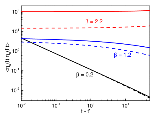
Figure 1: Autocorrelation function of the external nonequilibrium noise (11) for different values of the exponent $\beta$ as a function of the time difference $t-t^{\prime}$. The dashed and solid lines correspond to $t^{\prime}=10$ and $t^{\prime}=50$, respectively. For $\beta<1$ (black), the noise is stationary and its correlation function depends only on the time difference in the long-time limit. For $1<\beta<2$ (blue), the variance of the noise increases with time $t^{\prime}$ and its correlation function is nonstationary, i.e. explicitly dependent on $t^{\prime}$. Finally, for $\beta>2$ (red), the noise correlation function increases both as a function of the absolute time $t^{\prime}$ and of the difference $t-t^{\prime}$, indicating that the process is becoming more correlated with time.

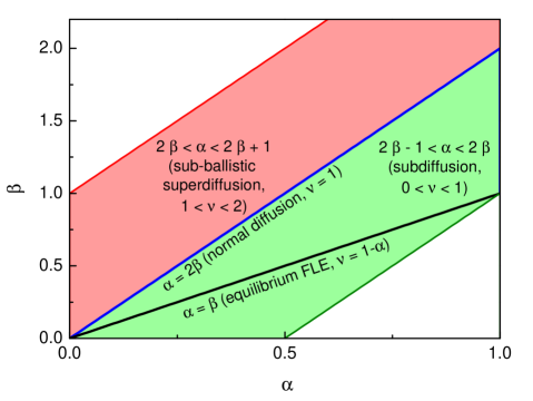
Figure 2: The diffusive phases due to the external noise as a function of the exponents $\alpha$ of the memory kernel and $\beta$ of the external noise. The shaded area corresponds to the experimentally relevant regime $0<\nu<2$.

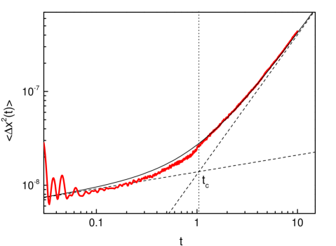
Figure 3: Comparison between the asymptotic result for the mean-square displacement (17) (black) and the numerical simulations of the Langevin equation (1) (red) for $\alpha=0.82$ and $\beta=2.13$. The transition from the subdiffusive equilibrium behavior (17) to superdiffusion is clearly visible and indicated by the dashed lines. The vertical dotted line marks the crossover time $t_{c}$, Eq. (18).

To compute the contribution of the external noise force to the mean-square displacement (6), we take the Laplace transform of Eq. (1) (for $F_{\rm p}=0$) and find,

$$m(s^{2}\tilde{x}(s) -sx_{0}-v_{0})=-\tilde{\gamma}(s)(s\tilde{x}(s)-x_{0})+\tilde{\eta}_{\rm i}(s)+\tilde{\eta}_{\rm e}(s),$$ (13)

where $x_{0}$, $v_{0}$ are the initial position and velocity. Solving for $\tilde{x}(s)$, we obtain the Laplace transform of the position autocorrelation,

$$\langle\tilde{x}(s)\tilde{x}(s^{\prime})\rangle=\langle\tilde{x}(s)\tilde{x}(s^{\prime})\rangle_{\rm i}+\tilde{g}(s)\tilde{g}(s^{\prime})\langle\tilde{\eta}_{\rm e}(s)\tilde{\eta}_{\rm e}(s^{\prime})\rangle,$$ (14)

where $\langle\tilde{x}(s)\tilde{x}(s^{\prime})\rangle_{\rm i}$ denotes the part of the correlation function due to the internal noise (we have here assumed that internal and external noise are statistically independent, since they have different sources). The kernel function $\tilde{g}(s)$ in Eq. (14) is defined as,

$$\tilde{g}(s)=\frac{1}{s(ms+\tilde{\gamma}(s))}.$$ (15)

The position autocorrelation in the time domain can be evaluated after Laplace inversion by using the correlation function (10). We find,

$$\langle x(t)x(t^{\prime})\rangle =\langle x(t)x(t^{\prime})\rangle_{\rm i}+D_{\beta}\int_{0}^{{\rm min}(t,t^{\prime})}dt^{\prime\prime}F(|t-t^{\prime}|+t^{\prime\prime})F(t^{\prime\prime})$$ (16)

with $$F(t)=\frac{1}{m}t^{\frac{\beta}{2}+1}E_{\alpha+1,\frac{\beta}{2}+1}\left(-\frac{\gamma_{\alpha}}{m}t^{\alpha+1}\right),$$

where $E_{a,b}(x)$ is the generalized Mittag-Leffler function [28]. The asymptotic behavior of the mean-square displacement, for $t=t^{\prime}\gg(m/\gamma_{\alpha})^{1/(\alpha+1)}$, then follows as,

$$\langle\Delta x^{2}(t)\rangle \simeq\langle\Delta x^{2}(t)\rangle_{\rm i}+\frac{D_{\beta}}{\gamma_{\alpha}^{2}}\frac{1}{\nu\Gamma^{2}\left(\frac{\nu+1}{2}\right)}t^{\nu},$$ (17)

with $\nu=\beta-2\alpha+1$. Here $\langle\Delta x^{2}(t)\rangle_{\rm i}$ is the equilibrium contribution to the mean-square displacement given by Eq. (6) and the second term on the right stems from the external noise. Comparing the two expressions, we see that for $\beta>\alpha$, the contribution from the external noise dominates for long times. The latter is subdiffusive for $\beta<2\alpha$ and superdiffusive for $\beta>2\alpha$ (see Fig. 2). For the experimentally observed values of the diffusion exponent $0<\nu<2$ [18, 15, 19, 25, 26, 13, 21], we have $2\alpha-1<\beta<2\alpha+1$. In Fig. 3, the asymptotic result for the mean-square displacement Eq. (17) is compared to those of numerical simulations of Eq. (1), showing excellent agreement.

To characterize the transition between the two diffusion regimes, we introduce the crossover time $t_{c}$, at which the contributions from the internal and external noise to the mean-square displacement (17) are of the same magnitude (see Fig. 3). Using Eq. (6), we find,

$$t_{c}=\left(\frac{2\nu\Gamma^{2}\left(\frac{\nu+1}{2}\right)}{\Gamma(2-\alpha)}\frac{k_{B}T\gamma_{\alpha}}{D_{\beta}}\right)^{\frac{1}{\nu+\alpha-1}}.$$ (18)

The equilibrium mean-square displacement (6) correctly describes the dynamics in the time window $(m/\gamma_{\alpha})^{1/(\alpha+1)}\ll t\ll t_{c}$, while the nonequilibrium external noise term dominates for $t\gg t_{c}$.

The behavior of the mean-square displacement (17) can be better understood by calculating the velocity autocorrelation function, which for long times is given by ($t>t^{\prime}$),

$$\langle v(t)v(t^{\prime})\rangle\simeq\langle v(t)v(t^{\prime})\rangle_{\rm i}+\frac{D_{\beta}}{\gamma_{\alpha}^{2}}\frac{1}{\pi}\Gamma(2-\nu)\sin\left(\pi\frac{\nu-1}{2}\right)(t-t^{\prime})^{\nu-2}.$$ (19)

Expression (19) is stationary and decays as a power law; it is negative for $\beta<2\alpha$ and positive for $\beta>2\alpha$. The latter correspond, respectively, to anticorrelated subdiffusion and correlated superdiffusion. The long-ranged nature of the velocity correlations is responsible for the anomalous dynamics of the system.

2 Nonequilibrium Stokes-Einstein relation

In contrast to the equilibrium internal noise force (2), the nonequilibrium external noise (11) may lead to a violation of the Stokes-Einstein relation (8). Indeed, if the external noise is more strongly correlated than the thermal noise ($\beta>\alpha$), the asymptotic behavior of the mean-square displacement is given by Eq. (17), which is no longer related to the response (7) via the temperature. However, we can establish a generalized Stokes-Einstein relation in the form,

$$\langle\Delta x^{2}(t)\rangle=2k_{B}T_{\rm eff}(t)J(t),$$ (20)

by introducing an effective time-dependent temperature,

$$k_{B}T_{\rm eff}(t) =\frac{D_{\beta}}{2\gamma_{\alpha}}\frac{\Gamma(2-\alpha)}{\nu\Gamma^{2}\left(\frac{\nu+1}{2}\right)}t^{\nu+\alpha-1}.$$ (21)

Effective temperatures are often used to measure how far away from equilibrium a system operates [29, 30]. For $\beta>\alpha$, Eq. (21) increases with time, indicating that the nonequilibrium properties of the system become more pronounced as time progresses. The latter can be understood by noting that the external noise injects energy into the system, driving it further away from equilibrium. For $\beta<\alpha$, the contribution from the external noise can be neglected asymptotically, and we have therefore $T_{\rm eff}=T$.

The introduction of the effective temperature (21) might at first glance appear purely formal. However, it gains physical significance by noting that it also measures the departure of the mean-square displacement (17) from its equilibrium expression (6). Indeed, for $t\ll t_{c}$, the effective temperature is equal to the actual physical temperature $T_{\rm eff}(t\ll t_{c})=T$, since the equilibrium contribution from the thermal noise dominates at short times (see Fig. 4). As a result, the asymptotic and transient behavior of the mean-square displacement are related via the effective temperature (21) as,

$$\langle\Delta x^{2}(t)\rangle=\frac{T_{\rm eff}(t)}{T}\langle\Delta x^{2}(t)\rangle_{t\ll t_{c}}.$$ (22)

Equations (20) and (22) provide two independent and complementary ways to determine the effective temperature: either by combining long-time active and passive measurements (as expressed by Eq. (20)), or by comparing short and long-time behavior in passive measurements alone (as indicated by Eq. (22)). Combining both equations, the transport properties of the system can thus be gained from passive measurements. The generalized Stokes-Einstein relation (20) with the effective temperature (21) therefore enable to connect passive and active microrheology in the nonequilibrium regime.

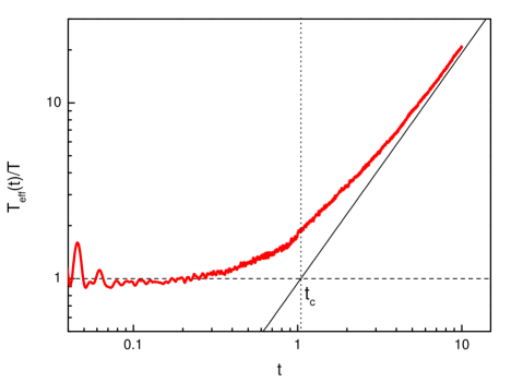
Figure 4: Time-dependent effective temperature $T_{\rm eff}(t)/T$ for $\alpha=0.82$ and $\beta=2.13$ ($\nu=1.49$). The red line is the result of numerical Langevin simulations, the solid black line corresponds to the asymptotic expression (21). For short times, $t\ll t_{c}$, $T_{\rm eff}(t)\simeq T$. On the other hand, the effective temperature grows as a power law with exponent $\nu+\alpha-1\simeq 1.31$ for long times, $t\gg t_{c}$.

In practice, system properties are often measured in frequency space by exerting a periodic force on the tracer particle [6, 17, 31]. It is thus desirable to define a frequency-dependent effective temperature. If the probe particle is acted on by a periodic force, $F_{\rm p}(t)=F_{0}\sin(\omega t)$, the response to this force may be characterized by the complex modulus $G(\omega)$, whose real and imaginary part describe the component of the force that is in-phase, respectively out-of-phase, with the response. From the expression (7) for the creep function, we find,

$$G^{\prime}(\omega) =\gamma_{\alpha}\omega^{1-\alpha}\sin\left(\pi\frac{\alpha}{2}\right),$$

$$G^{\prime\prime}(\omega) =\gamma_{\alpha}\omega^{1-\alpha}\cos\left(\pi\frac{\alpha}{2}\right).$$ (23)

As expected, the system behaves as a viscous liquid ($G^{\prime}=0$) for $\alpha=0$ and an elastic medium ($G^{\prime\prime}=0$) for $\alpha=1$. The sublinear frequency dependence of the modulus for low frequencies has been experimentally observed in Refs. [12, 31, 32]. For an equilibrium system, the imaginary part of the inverse complex modulus $G^{-1}(\omega)$ can be related to the power spectral density of the velocity $S_{v}(\omega)$ via,

$$S_{v}(\omega)=-2k_{B}T\omega[G^{-1}]^{\prime\prime}(\omega).$$ (24)

The latter is an expression of the fluctuation-dissipation relation in frequency space [14]. As before, this equilibrium relation can be generalized to the nonequilibrium case with external noise by introducing an effective temperature [33],

$$S_{v}(\omega) =-2k_{B}\mathcal{T}_{\rm eff}(\omega)\omega[G^{-1}]^{\prime\prime}(\omega).$$ (25)

Since the velocity process is stationary in the considered range of parameters $\alpha$ and $\beta$, its spectral density is given by the Fourier transform of its stationary autocorrelation function according to the Wiener-Khinchine theorem [14],

$$S_{v}(\omega)=\int_{-\infty}^{\infty}{\rm d}\tau\,e^{-i\omega\tau}\langle v(t+\tau)v(t)\rangle=\frac{D_{\beta}}{\gamma_{\alpha}^{2}}\omega^{1-\nu}.$$ (26)

As a consequence, we can identify the frequency-dependent effective temperature by comparing Eqs. (23) and (25). We find,

$$k_{B}\mathcal{T}_{\rm eff}(\omega) =\frac{D_{\beta}}{2\gamma_{\alpha}}\frac{1}{\cos\left(\pi\frac{\alpha}{2}\right)}\omega^{1-\nu-\alpha}.$$ (27)

The above definition of the effective temperature is equivalent to the one introduced for the mobility in Ref. [33]. Two other effective temperatures have been defined in a similar way, via the the spectral density of the position in Ref. [34] and via the spectral density of the noise in Ref. [13]. However, the latter are not suited to the superdiffusive, nonstationary regime as we will discuss below. The fact that $\mathcal{T}_{\rm eff}(\omega)$ increases with decreasing frequency for $\beta>\alpha$ indicates that the nonequilibrium properties of the system get more pronounced for low frequencies, corresponding to longer time scales, in complete analogy to the behavior of the effective temperature (21) in time; both measure the distance of the system from equilibrium.

In Eq. (25) the viscous modulus was related to the power spectral density of the velocity. Does a similar relation hold for the power spectral density of the position? For the subdiffusive regime $\beta<2\alpha$, the answer is yes; here, the two spectral densities are connected via,

$$\omega^{2}S_{x}(\omega)=S_{v}(\omega)\quad\text{for}\quad\beta<2\alpha.$$ (28)

Even though the position process is nonstationary (its variance increases with time), its power spectral density does not depend on time in this regime. However, in the superdiffusive regime $\beta>2\alpha$, the power spectral density now depends explicitly on time,

$$S_{x}(\omega,t)\simeq\frac{D_{\beta}}{\gamma_{\alpha}^{2}\nu\Gamma^{2}\left(\frac{\nu+1}{2}\right)}\omega^{-2}t^{\nu-1},$$ (29)

and cannot be related to the viscous modulus via a frequency-dependent temperature. Such a time-dependent spectral density is also found for the external noise (10):

$$S_{\eta_{\rm e}}(\omega,t)\simeq D_{\beta}\left\{\begin{array}[]{ll}\omega^{-\beta}&\text{for}\;\beta<2\\[4.30554pt] \frac{1}{(\beta-1)\Gamma^{2}\left(\frac{\beta}{2}\right)}\omega^{-2}t^{\beta-2}&\text{for}\;\beta>2.\end{array}\right.$$ (32)

The above unusual behavior is a direct consequence of the nonstationary properties of the external noise. For values of the noise exponent $0<\beta<1$, the noise correlation function is stationary, $\langle\eta_{\rm e}(t)\eta_{\rm e}(t^{\prime})\rangle\sim(t-t^{\prime})^{\beta-1}$ (see Eq. (12)), and its exponent is simply related to the exponent of the power spectral density $S_{\eta_{\rm e}}(\omega)\sim\omega^{-\beta}$ via the Wiener-Khinchine theorem. However, for $1<\beta<2$, even though the power spectral density is time independent, it would be wrong to conclude that the noise correlations also behave as $\langle\eta_{\rm e}(t)\eta_{\rm e}(t^{\prime})\rangle\sim(t-t^{\prime})^{\beta-1}$, since in this regime, the noise is actually nonstationary, and thus the Wiener-Khinchine relation no longer applies. Here, it is necessary to consider the full nonstationary noise correlation function (11).

3 Application to superdiffusion in living cells

Let us now apply our formalism to the description of anomalous diffusion in biological cells. The creep function and the mean-square displacement for muscle cells of adult mice were determined by means of active and passive microrheological measurements on the same sample in Ref. [13]. Sublinear growth of the creep function $J(t)\sim t^{0.18\pm 0.02}$ was observed, which corresponds to $\alpha=0.82\pm 0.02$ in our model. For an equilibrium system without external noise, one would thus expect $\langle\Delta x^{2}(t)\rangle\sim t^{\nu}$ with $\nu=0.18\pm 0.02$ from the Stokes-Einstein relation (8). This agrees well with the short-time behavior observed in the experiment, $\nu=0.12\pm 0.01$ [13]. For long times, however, the mean-square displacement was found to behave superdiffusively with an exponent $\nu=1.49\pm 0.06$. According to Eq. (17), this corresponds to $\beta=2.13\pm 0.08$ from the active measurement of the creep function and $\beta=2.25\pm 0.07$ from the passive measurement of the short-time behavior of the mean square displacement. Both values exhibit good agreement within the error margins, confirming the validity of the generalized Stokes-Einstein relation (20) connecting active and passive microrheology in the nonequilibrium regime.

The values of the diffusion exponent for short and long times appear to be universal for microrheological measurements performed on the cytoskeleton of a large class of cells [25, 26]: the short-time subdiffusion exponent is typically around $0.2$, whereas the superdiffusion exponent is around $1.6$. This corresponds to a value of $\beta\simeq 2.2$ in good agreement with the values stated above. The resulting parameter $\alpha\simeq 0.8$ also agrees with measurements of the viscoelastic modulus [31, 32]. The crossover time $t_{c}$ is found to be on the order of $1s$ [13, 26], and is therefore easily observed. The results of our analysis shows that the external noise is nonstationary for $\beta>2$ and that the noise power spectral density (32) is thus explicitly time-dependent, $S_{\eta}(\omega,t)\sim\omega^{-2}t^{\beta-2}$. The latter is in agreement with the $\omega^{-2}$ behavior of the intracellular stress fluctuations measured in Ref. [11] for a fixed time, and found in Ref. [35] for a model of the active cytoskeletal actin network. We emphasize that these findings cannot be reproduced using the stationary noise correlation (9) of Ref. [21]. In this experiment, $\beta\simeq 0.42$, a value corresponding to the stationary regime. The latter is due to a relatively large subdiffusion exponent $\nu$ close to 1, a value also observed in a couple of other experiments [18, 36].

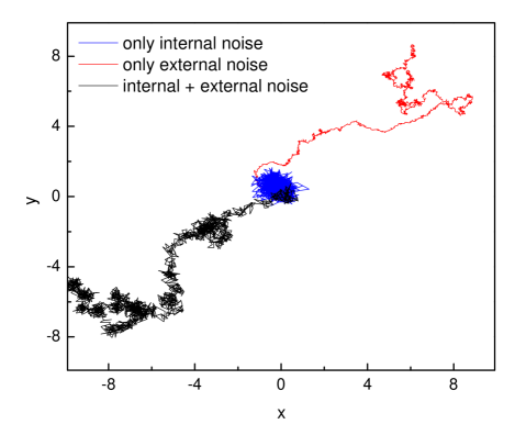
Figure 5: Typical trajectories obtained by simulating the fractional Langevin equation (1) for $\alpha=0.8$, $\beta=2.2$. The blue trajectory (center) corresponds to internal noise, the red one (top right) to external noise only. The black one (bottom left) is obtained for the combination of both noises. In the latter, the particle covers a large distance and, at the same time, explores its immediate surroundings. All trajectories start at the origin and have the same duration.

4 Discussion

Our model provides an extension of the fractional Langevin equation to describe anomalous diffusion in cells in the presence of nonequilibrium external noise. We have used the fact that the transient behavior in passive measurements is determined by the equilibrium properties to restore the connection between active and passive microrheology via a measurable effective temperature. We have confirmed the validity of the generalized Stokes-Einstein relation (20) by direct comparison with the experimental data of Ref. [13]. The observation that the response of living cells appears generic for a large class of cells [25, 26] hints at the widespread applicability of our formalism.

Typical trajectories obtained from numerical simulations of the Langevin equation are shown in Fig. 5. They exhibit remarkable similarity to experimentally observed trajectories [13, 15]. Under the sole action of the internal thermal noise, the particle thoroughly explores its immediate surroundings (blue trajectory). It has been shown that this subdiffusive motion is advantageous for reactions in the cell, leading to an increased probability of finding a nearby target site [37]. By contrast, in the presence of both internal (equilibrium) and external (nonequilibrium) noise, the dynamics becomes superdiffusive (black trajectory), and the particle covers large distances while still exploring the surrounding area. The latter allows for both fast transport and facilitated reactions—this last aspect is missing when only the nonequilibrium noise is present (red trajectory).

The origin of superdiffusion in living cells is thought to be the result of the collective behavior of molecular motors, switching on and off randomly, giving rise to correlated noisy motion [11, 12, 15]. A value of $\beta>2$ indicates that the external noise becomes slightly more correlated over time, as seen in Fig. 1. Our analysis thus suggests increasing cooperative action on part of the individual molecular motors in the nonstationary regime. An experimental confirmation of the resulting time-dependence of the power spectrum would therefore uncover some interesting new aspects of cell dynamics.

Acknowledgments: This work was supported by the Focus Area Nanoscale of the FU Berlin and the DFG (Contract No 1382/4-1). AD also thanks the Elsa-Neumann graduate funding for support.

References

- [1]
- [2] Gardel ML, Valentine MT, Weitz DA (2005). Microrheology. In Microscale Diagnostic Techniques, ed. KS Breuer, pp. 1-50. Berlin: Springer.
- [3] Wirtz D (2009) Particle-Tracking Microrheology of Living Cells: Principles and Applications. Annu. Rev. Biophys. 38: 301-326.
- [4] Squires TM, Mason TG (2010) Fluid Mechanics of Microrheology. Annu. Rev. Mater. Res. 42: 413-438.
- [5] Kollmannsberger P, Fabry B (2011) Linear and Nonlinear Rheology of Living Cells. Annu. Rev. Mater. Res. 41: 75-97.
- [6] Mason TG, Weitz DA (1995) Optical Measurements of Frequency-Dependent Linear Viscoelastic Moduli of Complex Fluids. Phys. Rev. Lett. 74: 1250-1253.
- [7] Mason TG, Ganesan K, van Zanten JH, Wirtz D, Kuo SC (1997) Particle Tracking Microrheology of Complex Fluids. Phys. Rev. Lett. 79: 3282-3285.
- [8] Schnurr B, Gittes F, MacKintosh FC, Schmidt CF (1997) Determining microscopic viscoelasticity in flexible and semiflexible polymer networks from thermal fluctuations. Macromolecules 30: 7781-7792.
- [9] Chen DT et al. (2003) Rheological Microscopy: Local Mechanical Properties from Microrheology. Phys. Rev. Lett. 90: 108301.
- [10] Brau RR et al. (2007) Passive and active microrheology with optical tweezers. J. Opt. A: Pure Appl. Opt. 9: 103-112.
- [11] Lau AWC, Hoffman BD, Davies A, Crocker JC, Lubensky TC (2003) Microrheology, Stress Fluctuations, and Active Behavior of Living Cells. Phys. Rev. Lett. 91: 198101.
- [12] Wilhelm C (2008) Out-of-Equilibrium Microrheology inside Living Cells. Phys. Rev. Lett. 101: 028101.
- [13] Gallet F, Arcizet D, Bohec P, Richert A (2009) Power spectrum of out-of-equilibrium forces in living cells: amplitude and frequency dependence. Soft Matter 5: 2947-2953.
- [14] Reif F (1965) Fundamentals of Statistical and Thermal Physics. New York: McGraw-Hill.
- [15] Bursac P et al. (2005) Cytoskeletal remodelling and slow dynamics in the living cell. Nat. Mater. 4: 557-561.
- [16] Mizuno D, Tardin C, Schmidt CF, MacKintosh FC (2007), Science 315: 370-373 .
- [17] Mizuno D, Head DA, MacKintosh FC, Schmidt CF (2008) Active and Passive Microrheology in Equilibrium and Nonequilibrium Systems. Macromolecules 41: 7194-7202.
- [18] Weiss M, Elsner M, Kartberg F, Nilsson T (2004) Anomalous Subdiffusion Is a Measure for Cytoplasmic Crowding in Living Cells. Biophys. J. 87: 3518-3524.
- [19] Golding I, Cox EC (2006) Physical Nature of Bacterial Cytoplasm. Phys. Rev. Lett. 96: 098102.
- [20] Brangwynne CP, Koenderink GH, MacKintosh FC, Weitz DA (2009) Intracellular transport by active diffusion. Trends Cell Biol. 19: 423-427.
- [21] Bruno L, Levi V, Brunstein M, Despósito MA (2009) Transition to superdiffusive behavior in intracellular actin-based transport mediated by molecular motors. Phys. Rev. E 80: 011912.
- [22] Mandelbrot BB, Van Ness JW (1968) Fractional Brownian Motions, Fractional Noises and Applications. SIAM Rev. 10: 422-437.
- [23] Lutz E (2001) Fractional Langevin equation. Phys. Rev. E 64: 051106.
- [24] Pottier N (2003) Aging properties of an anomalously diffusing particule. Physica A 317: 371-382.
- [25] Trepat X et al. (2007) Universal physical responses to stretch in the living cell. Nature 447: 592-596.
- [26] Trepat X, Lenormand G, Fredberg JJ (2008) Universality in cell mechanics. Soft Matter 4: 1750-1759.
- [27] Abramowitz M, Stegun IA (1964) Handbook of Mathematical Functions: With Formulas, Graphs, and Mathematical Tables. Mineola: Dover.
- [28] Bateman H, Erdélyi A (1955) Higher Transcendental Functions Vol III. New York: McGraw-Hill.
- [29] Cugliandolo LF, Kurchan J, Peliti L (1997) Energy flow, partial equilibration, and effective temperatures in systems with slow dynamics. Phys. Rev. E 55: 3898-3914.
- [30] Cugliandolo LF (2011) The effective temperature. J. Phys. A: Math. Theor. 44: 483001.
- [31] Hoffman BD, Crocker JC (2009) Cell Mechanics: Dissecting the Physical Responses of Cells to Force. Annu. Rev. Biomed. Eng. 11: 259-288.
- [32] Massiera G, Van Citters KM, Biancaniello PL, Crocker JC (2007) Mechanics of Single Cells: Rheology, Time Dependence, and Fluctuations. Biophys. J. 93: 3703-3713.
- [33] Pottier N (2005) Out of equilibrium generalized Stokes-Einstein relation: determination of the effective temperature of an aging medium. Physica A 345: 472-484.
- [34] Jabbari-Farouji S et al. (2008) Effective temperatures from the fluctuation-dissipation measurements in soft glassy materials. Europhys. Lett. 84: 20006.
- [35] MacKintosh FC, Levine AJ (2008) Nonequilibrium Mechanics and Dynamics of Motor-Activated Gels. Phys. Rev. Lett. 100: 018104.
- [36] Tseng T, Kole TP, Wirtz D (2002) Micromechanical Mapping of Live Cells by Multiple-Particle-Tracking Microrheology Biophys. J. 83: 3162-3176.
- [37] Guigas G, Weiss M. (2008) Sampling the Cell with Anomalous Diffusion? The Discovery of Slowness Biophys. J. 94: 90-94.