Abstract Geometrical Computation 8:
Small Machines, Accumulations & Rationality

Abstract

In the context of abstract geometrical computation, computing with colored line segments, we study the possibility of having an accumulation with small signal machines, i.e., signal machines having only a very limited number of distinct speeds. The cases of $2$ and $4$ speeds are trivial: we provide a proof that no machine can produce an accumulation in the case of $2$ speeds and exhibit an accumulation with $4$ speeds.

The main result is the twofold case of $3$ speeds. On the one hand, we prove that accumulations cannot happen when all ratios between speeds and all ratios between initial distances are rational. On the other hand, we provide examples of an accumulation in the case of an irrational ratio between two speeds and in the case of an irrational ratio between two distances in the initial configuration.

This dichotomy is explained by the presence of a phenomenon computing Euclid’s algorithm ($\gcd$): it stops if and only if its input is commensurate (i.e., of rational ratio).

Keywords

Abstract Geometrical Computation; Signal Machine; Accumulation; Unconventional Computing; Euclid’s Algorithm.

¹ Univ. Orléans, ENSI de Bourges, LIFO ÉA 4022, F-45067 Orléans, France

² CESI-IRISE, 959 rue de la Bergeresse, F-45160 Olivet, France

1 Introduction

Imagine yourself with some color pencils and a sheet of paper together with ruler and compass. There is something drawn in a corner of the paper and you are given rules so as to extend the drawing. According to the rules and the initial drawing/configuration you might stop soon, have to extend the paper indefinitely or draw forever in a bounded part of the paper as on top of Fig. 1(a). Already on this simple setting emerges the usual questions related to dynamical systems: liveness, unbounded orbit or convergence/accumulation.

In this article we concentrate on accumulation in the case where the dynamical system is a signal machine in the context of abstract geometrical computation. In this setting, one drawing direction is distinguished and used as time axis. Line segments are enlarged synchronously until they intersect another one. This goes on until no more collision can happen.

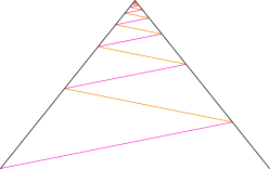
(a) Most basic accumulation.

(b) $1$ speed: no collision.

(c) $2$ speeds: no accumulation.

Figure 1: Basic cases.

The line segments are the traces of signals and their intersections are collisions of signals. Each signal corresponds to some meta-signal. In-coming signals are removed and new ones are emitted according to the meta-signals associated with the incoming signals. This is called a collision rule. Signals that correspond to the same meta-signal must travel at the same speed, the resulting traces are parallel. There are finitely many meta-signals so there are finitely many collision rules.

The signals move on a one dimensional Euclidean space orthogonal to the temporal axis (in the figures, space is horizontal and time elapses upwards). Considering the traces leads to two dimensional drawings called space-time diagrams (as illustrated throughout the article). Please let us point out that space and time are continuous spaces (the real line) and that signals as well as collisions are dimensionless points. Computations are exact, there is no noise nor approximation.

Signal machines are very powerful and colorful complex systems. Accumulation is easy to achieve and is in fact the cornerstone to hypercomputation in the model [Durand-Lose, 2009a]. In the present article, we investigate the minimum size of a machine so that an accumulation is possible or not. Already with four meta-signals of different speeds (or directions on the drawing) an accumulation can happen as depicted on Fig. 1(a).

In fact, we will see in the sequel of this article that the number of meta-signals is not relevant; the relevant measure here is the number of different speeds and in the case of three speeds, their values and the initial positions as explained below. One speed does not even allow any collision (see Fig. 1(b)). With two speeds, the number of collisions is finite and signals have to follow a regular grid which has no accumulation (see Fig. 1(c)).

When three signals of different speeds are present, in order to make accumulations more likely to occur, we can imagine that each collision generates all signals. Then, in the generated space-time diagrams, we can exhibit the emulation of Euclid’s algorithm to compute some greatest common divisor ($\gcd$). If the ratios involved are irrational, then the algorithm does not stop and brings forth an accumulation. On the contrary, if every ratio that could be involved in a $\gcd$ computation is rational, then a global $\gcd$ is generated and some global regular mesh emerges. Whatever the number of meta-signals and whatever the collision rules are, there is no way for the signals to escape this mesh. The signals have to be on the mesh and the mesh does not have any accumulation point. Hence, the diagram cannot have an accumulation.

State of the art

Signal machines are one of the (unconventional) models of computation dealing with Euclidean geometry. To name a few, one can think of: Euclidean abstract machines [Mycka et al., 2006, Huckenbeck, 1989], piecewise constant derivatives systems [Bournez, 1997], colored universes [Jacopini and Sontacchi, 1990]…

Signal machines were originally introduced as a continuous counterpart of cellular automaton to provide a context for the underlying Euclidean reasoning often found in the discrete cellular automata literature as well as propose an abstract formalization of the concept of signal [Durand-Lose, 2008b, Mazoyer, 1996, Mazoyer and Terrier, 1999].

Signal machines are able to compute in the classical Turing understanding. This paper is somehow a companion to [Durand-Lose, 2011] where a Turing-universal signal machine is presented with only $13$ meta-signals and $4$ speeds. This research takes place in the quest for minimality in order to compute, and thus get unpredictable behavior. Let us cite [Rogozhin, 1996, Woods and Neary, 2007] for Turing machines, [Cook, 2004, Ollinger and Richard, 2011] for cellular automata, and [Margenstern, 2000] for a more general picture.

Being in a continuous setting, signal machines can carry out analog computations in the sense of both the BSS’s model [Blum et al., 1989, Durand-Lose, 2008a] and Computable analysis [Weihrauch, 2000, Durand-Lose, 2009b].

Massive parallelism and the capability to approximate a fractal (with potentially infinitely many accumulations) allows to provide efficient solutions to hard problems: SAT for the class NP [Duchier et al., 2010] and Q-SAT for PSPACE [Duchier et al., 2012]. From previous work on signal machine, accumulations are known to be easy to generate. They are a powerful tool to accelerate a computation and provide hypercomputation [Durand-Lose, 2009a]. Recently, it has been proved that, starting from a rational machine and configuration, the locations of isolated accumulations have to be d-c.e (difference of computably enumerable) real numbers and that any such number can be reached [Durand-Lose, 2012].

Outline

Formal definitions of signal machines, their dynamics, space-time diagrams, properties and normalizations are given in Sec. 2, as well as an introductory example: the computation of the remainder of Euclidean division (later embedded inside the $\gcd$ computation). In Sec. 3, the case of two and four speeds are settled. Section 4 studies the case of three speed systems, where the rationality of ratios enters into play. With an irrational ratio in distances (resp. in speeds), an accumulation is susceptible to happen, this is proven by following the steps of Euclid’s algorithm into the space-time diagram and proving that the accumulation occurs in finite time. Otherwise, if all ratios are rational, then we prove that all generated signals must be on a regular mesh, this mesh has no accumulation, so that the initial space-time diagram cannot have any. Section 5 concludes this paper.

2 Signal machines

This section introduces basic definitions about signal machines and their space-time diagrams, with several formulations: in terms of machines, topology and dynamics. Subsect. 2.2 gives two toy examples —geometrical computation of a substraction and a modulo— that will be used to implement Euclid’s algorithm with signals. Some notions and geometrical properties such as affine transformations of machines and inclusions of diagrams are given in Subsect. 2.3.

2.1 Definitions

We formalize here the definition of a signal machine, which corresponds to a set of meta-signals, a speed function assigning a real speed to each meta-signal and a function describing the result of a meta-signals collision:

Definition 1 (Signal machine).

A signal machine $\mathfrak{M}$ is a triplet $\mathfrak{M}=(\mathcal{M},\mathcal{S},\mathcal{R})$ where:

1. $\mathcal{M}$ is a finite set of meta-signals;

2. $\mathcal{S}:\mathcal{M}\to\mathbb{R}$ is the speed function which assigns a real speed value $\mathcal{S}(\mu)$ to each meta-signal $\mu$;

3. $\mathcal{R}:\mathcal{P}(\mathcal{M})\to\mathcal{P}(\mathcal{M})$ is the collision function: each set of meta-signals $C^{-}\in\mathcal{P}(\mathcal{M})$ such that $|C^{-}|\geq 2$ and $\mathcal{S}_{\restriction C^{-}}$ is $injective$, is mapped to a set of meta-signals $C^{+}$ so that $\mathcal{S}_{\restriction C^{+}}$ is $injective$.

Figure 2 provides an example of a very simple signal machine, and an evolution of this machine, that we call a space-time diagram. The meta-signals are listed in Fig. 2(a), and collision rules are given by Fig. 2(c). Figure 2(b) provides an example of a space-time diagram for this machine.

Name	Speed
s1	$1$
s2	$-1/2$
s3	$3$
s4	$0$

(a) Meta-signals.

(b) Space-time diagram.

$\{\textsf{\sf{s${}_{2}$}},\textsf{\sf{s${}_{1}$}}\}$ $\rightarrow$	$\{\textsf{\sf{s${}_{2}$}},\textsf{\sf{s${}_{1}$}},\textsf{\sf{s${}_{3}$}}\}$
$\{\textsf{\sf{s${}_{3}$}},\textsf{\sf{s${}_{4}$}}\}$ $\rightarrow$	$\{\textsf{\sf{s${}_{2}$}}\}$

(c) Collision rules.

Figure 2: Example of a signal machine and one of its possible evolution.

Condition (iii) of $\mathcal{R}$ definition means that signals can collide only if they have distincts speeds, and a collision involves at least two signals. The signals resulting from a collision must also have distinct speeds. Since we interpret $\mathcal{R}(C^{-})=C^{+}$ as a rule, we rather note $C^{-}\rightarrow C^{+}$ instead of $\mathcal{R}(C^{-})=C^{+}\enspace$.

We call $n$-speed machine any signal machine having exactly $n$ distinct values for its meta-signals speeds, i.e., $\mathfrak{M}$ is a $n$-speed machine if $|\mathcal{I}m(\mathcal{S})|=n\enspace$.

Configurations

A configuration is a function from the real line (space) into the set of meta-signals and collision rules plus two extra values: $\oslash$ (for nothing there) and ✺ (for accumulation). We note $\mathcal{V}$ the set of values, i.e., $\mathcal{V}=\mathcal{M}\cup\mathcal{R}\cup\{\oslash\}\cup\{\text{\char 90}\}$. A configuration can be seen as the “global state” of the signal machine at a given time, and describes the presence and the disposition of signals and collisions in the space $\mathbb{R}$.

Any signal or collision must be spatially isolated: there is nothing else but $\oslash$ arbitrarily closed. The accumulation points of non-$\oslash$ locations must be ✺. These are spatial static accumulations.

Definition 2 (Configuration).

A configuration, $c$, is a function from the real line into meta-signals, rules, $\oslash$ and ✺ (let $\mathcal{V}=\mathcal{M}\cup\mathcal{R}\cup\{\oslash,\text{\char 90}\}$ so that $c:\mathbb{R}\rightarrow\mathcal{V}$) such that:

1. all signals and collisions are isolated:
   $\forall x\in\mathbb{R},\ c(x)\in\mathcal{M}\cup\mathcal{R}\ \Rightarrow\exists\varepsilon>0,\ \forall y,\ 0<|x-y|<\varepsilon\Rightarrow c(y)=\oslash\enspace$;

2. spatial accumulation are marked accordingly: any $x$ that is an accumulation point of $c^{-1}(\mathcal{V}\setminus\{\oslash\})$ verifies $c(x)=\text{\char 90}$ ($x$ in $\mathbb{R}$ is an accumulation point of a subset E of $\mathbb{R}$ iff $\forall\varepsilon$, $1<|E\cap(x-\varepsilon,x+\varepsilon)|$).

If there is a signal of speed $s$ at $x$, then, unless there is a collision before, after a duration $\Delta t$, its position is $x+s{\cdot}\Delta t$. At a collision, all incoming signals are immediately replaced by outgoing signals in the following configurations according to collision rules.

For the next definition, the support of a configuration $c$ will denote the set of non-$\oslash$-valued positions, i.e., $support(c)=\{x\in\mathbb{R}~{}|~{}c_{0}(x)\neq\oslash\}$.

Definition 3 (Initial configuration).

An initial configuration is a configuration $c_{0}:\mathbb{R}\rightarrow\mathcal{V}$ so that:

1. the support of $c_{0}$ is finite, i.e., $\{x\in\mathbb{R}~{}|~{}c_{0}(x)\neq\oslash\}$ is finite;

2. for all $x\in\mathbb{R}$, $c_{0}(x)\neq\text{\char 90}\enspace$.

Accumulations (the ✺ values) are forbidden in the initial configuration. The case of an initial collision is interpreted by the possibility of having several signals with distinct speeds at the same initial position: for an initial collision $\{\mu_{1},\ldots,\mu_{p}\}\rightarrow\{\mu_{1}^{\prime},\ldots,\mu_{q}^{\prime}\}$ occuring at position $x$, we rather note $[\mu_{1}^{\prime},\ldots,\mu_{q}^{\prime}]@x$ or $\mu_{1}^{\prime}@x,\ldots,\mu_{q}^{\prime}@x$. In this way, an initial configuration can be expressed only in terms of signals at some positions (the other positions taking the value $\oslash$). So we can give an initial configuration $c_{0}$ by a finite set of the form $c_{0}=\{\mu_{1}@x_{1},\ldots,\mu_{k}@x_{k}\}\enspace$ where $\mu_{i}@x_{i}$ means $\mu_{i}$ is initially located at the spatial position $x_{i}$ i.e. $c_{0}(x_{i})=\mu_{i}$.

We insist that $[\mu_{1}^{\prime},\ldots,\mu_{q}^{\prime}]@x=\mu_{1}^{\prime}@x,\ldots,\mu_{q}^{\prime}@x$ is just a notation to simplify the writing of collisions when we express a configuration as a set of non-$\oslash$ values. But by definition, a configuration $c$ is a function from $\mathbb{R}$ in $\mathcal{V}$: for each $x\in\mathbb{R}$, the value $c(x)$ is unique (and is either a meta-signal, a collision, ✺ or $\oslash$). We will also use this notation of collision in any configuration (and not only for an initial one), and $c_{t}=\{\mu_{1}^{\prime}@x,\ldots,\mu_{q}^{\prime}@x\}$ has to be interpreted by “any collision producing $\{\mu_{1},\ldots,\mu_{q}^{\prime}\}$ and occuring at $x$”, i.e., $c_{t}(x)=C$ with $C^{+}=\{\mu_{1}^{\prime},\ldots,\mu_{q}^{\prime}\}$. We allow initial configurations (and only initial configurations) to contain some signals of distinct speeds at the same initial position, even if this set of signals doesn’t correspond to a collision outcoming set of signals.

Definition 4 (Rational signal machine).

A signal machine is rational if all speeds are rational numbers and non-$\oslash$ positions in the initial configuration are also rational numbers.

Since the position of collisions are solutions of rational linear equations systems, they are rational. In any space-time diagram of a rational signal machine, as long as there is no accumulation, the coordinates of all the collisions are rational.

Definition 5 (Rational-like).

A signal machine is rational-like if all its speeds are two-by-two commensurate, i.e., all ratios between speeds are rationnal. A configuration is rational-like if all distances are two-by-two commensurate.

This means that a signal machine is rational-like if all its speeds are rational up to a multiplicative coefficient. In particular, any rational machine is rational-like.

Space-time diagrams

A space-time diagram can be formulated in a topological way, based on the classical topology of $\mathbb{R}^{2}$, whose open sets are generated by the Euclidean distance. The topological formulation of diagram implies that space and time are considered like a whole object —the space-time structure— and there is a priori no dynamics.

We define first a notion that will be used to define accumulation: the notion of causal past of a point.

Definition 6 (Causal past and isolated accumulation).

Let $\nu_{max}$ (maximal right speed) and $\nu_{min}$ (maximal left speed) be the maximum and minimum values taken by the speed function $\mathcal{S}$. The value at position $(x,t)$ in the space-time diagram only depends on the values at the position on the causal past or backward light cone:

$$\Gamma^{-}(x,t)=\left\{\rule{0.0pt}{11.00008pt}\,(x^{\prime},t^{\prime})\,\middle|\,t^{\prime}<t\wedge\nu_{max}{\cdot}(t^{\prime}{-}t)<x^{\prime}-x<\nu_{min}{\cdot}(t^{\prime}{-}t)\,\right\}\enspace.$$

This notion is illustrated in Fig. 3(a).

We can now give the formalization of space-time diagrams:

Definition 7 (Space-time diagram).

A space-time diagram is a map $\mathbb{D}$ from a time interval $[0,T]\subset\mathbb{R^{+}}$ ($T$ can be infinite) to the set of configurations (i.e. $\mathbb{D}$ can be identified to a map $\mathbb{R}\times\mathbb{R^{+}}\to\mathcal{V}$) such that:

1. $\forall t\in[0,T]\ \{x\in\mathbb{R}\ |\ c_{t}(x)\neq\oslash\}$ is finite;

2. if $c_{t}(x)=\mu\in\mathcal{M}$ then $\exists t_{i},t_{f}\in[0,T]$ with $t_{i}<t<t_{f}$ or $0=t_{i}=t<t_{f}$ or $t_{i}<t=t_{f}=T$ such that:

   • $\forall t^{\prime}\in~{}]t_{i},t_{f}[\ c_{t^{\prime}}(x+\mathcal{S}(\mu)(t-t^{\prime}))=\mu$,

   • $t_{i}=0$ or $c_{t_{i}}(x_{i})\in\mathcal{R}$ and $\mu\in(c_{t_{i}}(x_{i}))^{+}$ where $x_{i}=x+\mathcal{S}(\mu)(t_{i}-t)$,

   • $t_{f}=T$ or $c_{t_{f}}(x_{f})\in\mathcal{R}$ and $\mu\in(c_{t_{f}}(x_{f}))^{-}$ where $x_{f}=x+\mathcal{S}(\mu)(t_{f}-t)$;

3. if $c_{t}(x)=C^{-}\rightarrow C^{+}\in\mathcal{R}$ then $\exists\ \varepsilon>0\ \forall t^{\prime}\in[t-\varepsilon,t+\varepsilon]\ \forall x^{\prime}\in[x-\varepsilon,x+\varepsilon]$

   • $c_{t^{\prime}}(x^{\prime})\in C^{-}\cup C^{+}\cup\{\oslash\}$,

   • $\forall\mu\in C^{-}\ :(\ c_{t^{\prime}}(x^{\prime})=\mu\ )\Leftrightarrow(\ t<t^{\prime}\text{ and }x^{\prime}=x+\mathcal{S}(\mu)(t^{\prime}-t)\ )$,

   • $\forall\mu\in C^{+}\ :(\ c_{t^{\prime}}(x^{\prime})=\mu\ )\Leftrightarrow(\ t^{\prime}<t\text{ and }x^{\prime}=x+\mathcal{S}(\mu)(t^{\prime}-t)\ )$;

4. if $c_{t}(x)=\text{\char 90}$ then

   • $\exists\ \varepsilon>0\ \forall(x^{\prime},t^{\prime})\notin\Gamma^{-}(x,t)$ s.t. $|x-x^{\prime}|<\varepsilon,\ |t-t^{\prime}|<\varepsilon$ we have $c_{t^{\prime}}(x^{\prime})=\oslash$,

   • $\forall\ \varepsilon>0,\ |\{\ (x^{\prime},t^{\prime})\in\Gamma^{-}(x,t)\ |\ t-\varepsilon<t^{\prime}<t\wedge c_{t^{\prime}}(x^{\prime})\in\mathcal{R}\ \}|=\infty\enspace$.

As done for configurations, we can define the support of a diagram $\mathbb{D}$ by $support(\mathbb{D})=\{(x,t)\in\mathbb{R}\times\mathbb{R^{+}}~{}|~{}\mathbb{D}(x,t)\neq\oslash\}$.

Equivalent diagrams

To formalize the idea that two geometrical computations are “the same”, we define the notion of equivalent diagrams. Intuitively, two diagrams are equivalent if they have the same structure, i.e., the same causality links between their respective collisions and signals, independently of their positions or the meta-signal names. We formalize such an invariancy of structure with the notion of homeomorphism: a diagram obtained by a continuous transformation will keep the same structure.

Definition 8 (Equivalent diagrams).

Let $\mathbb{D}$ and $\mathbb{D}^{\prime}$ two space-time diagrams with respective value sets $\mathcal{V}=\mathcal{M}\cup\mathcal{R}\cup\{\oslash,\text{\char 90}\}$ and $\mathcal{V}^{\prime}=\mathcal{M}^{\prime}\cup\mathcal{R}^{\prime}\cup\{\oslash,\text{\char 90}\}$. We say that $\mathbb{D}$ and $\mathbb{D}^{\prime}$ are equivalent if:

1. there is an homeomorphism $h:\mathbb{R}\times\mathbb{R^{+}}\to\mathbb{R}\times\mathbb{R^{+}}$, and

2. there is a bijection $\Phi:\mathcal{V}\to\mathcal{V}^{\prime}$ so that $\Phi[\mathcal{M}]=\mathcal{M}^{\prime}$, $\Phi[\mathcal{R}]=\mathcal{R}^{\prime}$, $\Phi(\text{\char 90})=\text{\char 90}$ and $\Phi(\oslash)=\oslash$ and so that $\forall\mu\in\mathcal{M},\forall\rho\in\mathcal{R},\ \,\mu\in C^{-}\ (resp.C^{+})\Rightarrow\Phi(\mu)\in\Phi(\rho)^{-}\ (resp.\Phi(\rho)^{+})$,

satisfying $\forall(x,t)\in\mathbb{R}\times\mathbb{R^{+}},\ \mathbb{D}^{\prime}(x,y)=\Phi(\mathbb{D}(h(x,y)))$.

The second condition means that $\Phi$ induces a bijection from the sets of meta-signals of $\mathbb{D}$ into the set of meta-signals of $\mathbb{D}^{\prime}$ and from the set of rules of $\mathbb{D}$ to the set of rules of $\mathbb{D}^{\prime}$ so that the place of meta-signals into the rules is kept.

Dynamics

We give a presentation of a machine evolution in terms of dynamics. This definition has been introduced by [Durand-Lose, 2012], in which it has been used to characterize the exact coordinates of isolated accumulations.

Definition 9 (Dynamics).

Considering a configuration $c$, the time to the next collision, $\Delta(c)$, is equal to the minimum of the positive real numbers $d$ such that:

$$\exists x_{1},x_{2}\in\mathbb{R},\exists\mu_{1},\mu_{2}\in\mathcal{M}\left\{\begin{array}[]{l@{}}x_{1}+d{\cdot}\mathcal{S}(\mu_{1})=x_{2}+d{\cdot}\mathcal{S}(\mu_{2})\\ c(x_{1})=\mu_{1}\vee(c(x_{1})=C^{-}\rightarrow C^{+}\wedge\mu_{1}\in C^{+})\\ c(x_{2})=\mu_{2}\vee(c(x_{2})=C^{-}\rightarrow C^{+}\wedge\mu_{2}\in C^{+})\end{array}\right.\enspace.$$

It is $+\infty$ if there is no such $d$.

Let $c_{t}$ be the configuration at time $t$; for $t^{\prime}$ between $t$ and $t+\Delta(c_{t})$, the configuration at $t^{\prime}$ is defined as follows. First, signals are set according to $c_{t^{\prime}}(x^{\prime})=\mu$ iff $c_{t}(x)=\mu\vee(c_{t}(x)=C^{-}\rightarrow C^{+}\wedge\mu\in C^{+})$ where $x=x^{\prime}+(t{-}t^{\prime}){\cdot}\mathcal{S}(\mu)$. There is no collision to set ($t^{\prime}$ is before the next collision). Then (static) accumulations are set: $c_{t^{\prime}}(x^{\prime})=\text{\char 90}$ iff $x^{\prime}$ is an accumulation point of $c_{t^{\prime}}^{-1}(\mathcal{M})$. It is $\oslash$ everywhere else.

For the configuration at $t^{\prime}=t+\Delta(c_{t})$, collisions are set first: $c_{t^{\prime}}(x^{\prime})=C^{-}\rightarrow C^{+}$ iff for all $\mu\in C^{-}$, $c_{t}(x_{\mu})=\mu\vee(c_{t}(x_{\mu})=C^{-}\rightarrow C^{+}\wedge\mu\in C^{+})$ where $x_{\mu}=x^{\prime}+(t{-}t^{\prime}){\cdot}\mathcal{S}(\mu)$. Then meta-signals are set (where there is not already a collision), and finally (static) accumulations.

The sequence of collision time is defined by: $t_{0}=0$, $t_{n+1}=t_{n}+\Delta(c_{t_{n}})$. This sequence is finite if there is an $n$ such that $\Delta(c_{t_{n}})=+\infty$. Otherwise, since it is non-decreasing, it admits a limit. If the sequence is finite or its limit is infinite, then the whole space-time diagram is defined. These cases are of no interest here since there are no non-static accumulations.

Only the last case is considered from now on: there is a finite limit, say $\tilde{t}$. The configuration at $\tilde{t}$ is defined as follows. First (dynamic) accumulations are set: $c_{\tilde{t}}(x)=\text{\char 90}$ iff $\forall\varepsilon>0\$ then there exists $x^{\prime}$ and $t^{\prime}$ such that $|x-x^{\prime}|<\varepsilon$, $\tilde{t}-\varepsilon<t^{\prime}<\tilde{t}$ and $c_{t^{\prime}}(x^{\prime})\in\mathcal{R}$. Then collisions are set: $c_{\tilde{t}}(x)=C^{-}\rightarrow C^{+}$ iff for all $\mu\in C^{-}$, $\exists\varepsilon$, $\forall\varepsilon^{\prime}$, $0{<}\varepsilon^{\prime}{<}\varepsilon$, holds $c_{\tilde{t}-\varepsilon^{\prime}}(x^{\prime}-\varepsilon^{\prime}{\cdot}\mathcal{S}(\mu))=\mu$. Then meta-signals are set: $c_{\tilde{t}}(x)=\mu$ iff $\exists\varepsilon$, $\forall\varepsilon^{\prime}$, $0{<}\varepsilon^{\prime}{<}\varepsilon$, then $c_{\tilde{t}-\varepsilon^{\prime}}(x^{\prime}-\varepsilon^{\prime}{\cdot}\mathcal{S}(\mu))=\mu$. Finally, static accumulations are set.

At each time, a position is set only if it is not already set. At the end every unset position is assigned by $\oslash$. The dynamics is uniform in both space and time. Please note that this definition does not always define an extension to the computation (when there are infinitely many signals, $\Delta(c)$ is an infimum that could be equal to zero), nevertheless it does, in the cases considered here. Figure 3(b) illustrates the sequence of collision times for the previously given in example.

(a) Causal past or backward light cone.

(b) First collision times of the diagram of Fig. 2(b).

Figure 3: Example of a space-time diagram and causal past.

Notations

In the whole paper, $\mathfrak{M}$ will always designate a signal machine, and the function (resp. the parameters) of the machine can be indicated as index (resp. exponent). For instance, $\mathfrak{M}_{2}^{a,b}$ will designate a $2$-speed machine, having its speed values equal to $a$ and $b$. A signal name will be noted in sf font, and the sign of its speed will be indicated by a right or left overlined arrow. Configurations at time $t$ will always be noted by $c_{t}$, and some parameters can be expressed as exponent, e.g., $c_{0}^{x}$ stands for an initial configuration in which the value $x$ is used for some positions. The notations $\mathbb{D}$ and $\mathcal{V}$ respectively represent diagrams and diagrams values, i.e., $\mathcal{V}$ is the set $\mathcal{M}\cup\mathcal{R}\cup\{\oslash\}\cup\{\text{\char 90}\}$.

2.2 A 3-speed toy example: computing the modulo

When considering small signal machines, that is with few distinct speeds, one natural question is whether such machines can still process meaningful computations. As a matter of fact, we may see in Sec. 3.2 that allowing only two distinct speeds is too restrictive.

In this section, we provide two detailed (yet informal) examples of 3-speed machines illustrating our computational model on simple practical algorithms. Those two machines geometrically compute the subtraction and modulo operators, respectively, between two positive reals.

The notions of euclidean division, modulo and greatest common divisor (which will be used in Sec. 4.1), usually defined above integers, are generalized here to real numbers in a natural way. More precisely, for $a,b\in\mathbb{R}$, the euclidean division (or integer division) of $a$ by $b$ is the unique $n\in\mathbb{Z}$ (given by $\lfloor\frac{a}{b}\rfloor$) so that $a=b\cdot n+r$, where $r\in\mathbb{R}$ and $0\leq r<|b|$. The remainder $r$ defines the value of $a$ modulo $b$, noted by $a\bmod b$. We say that the real number $b$ divides the real number $a$ if $a\bmod b=0$. The greatest common divisor of two reals $a$ and $b$, denoted by $\gcd(a,b)$, is the greatest real which divides both $a$ and $b$. By now, we will only consider positive real numbers, since divisions, modulo and $\gcd$ of any reals can easily be deduced from those of their absolute values.

Geometrical encoding of a value

There may be several ways to geometrically encode values in a signal machine. In this article, we choose to encode any value $x\neq 0$ (integer or real) by the distance between two stationary signals w₀ and w_x (where w stands for “wall”), the stationary signal w₀ being unique and common to every encoded value.

A 3-speed machine for the subtraction

We first illustrate our computational model by constructing a 3-speed machine $\mathfrak{M}_{sub}$ computing a single subtraction $a-b$ between two positive values $a$ and $b$. For the sake of comprehension, we suppose $a>b$.

We define meta-signals and collision rules in order to implement the following idea. The two positive values $a$ and $b$ are encoded by the distance between a common stationary meta-signal w₀ and respective stationary meta-signals w_a and w_b, as explained above. Using several temporary meta-signals of speed $-1$ and $1$ ($\overrightarrow{\textsf{\sf{zig}}}$, $\overleftarrow{\textsf{\sf{zag}}}$, $\overrightarrow{\textsf{\sf{ZIG}}}$, $\overleftarrow{\textsf{\sf{ZAG}}}$), we geometrically copy the distance between w₀ and w_b, which represents the value $b$, and shift the signal w_a to the left by this exact distance (which is then renamed w_r as being the result of the subtraction operation). The initial configuration is set to $c_{0}^{a,b}=\{\overrightarrow{\textsf{\sf{init}}}@{-1},\textsf{\sf{w${}_{0}$}}@0,\textsf{\sf{w${}_{b}$}}@b,\textsf{\sf{w${}_{a}$}}@a\}$.

Using basic geometry notions and observing that the signals shifting operation defines a parallelogram on the machine’s diagram, one can easily prove that the position of the signal w_r is such that the distance between w₀ and w_r corresponds exactly to $r=a-b$. The definition of this machine is given in Fig. 4(a), and we give a run example of this machine for values $a=11$ and $b=3$ in Fig. 4(b).

Meta-signals Speeds $\overrightarrow{\textsf{\sf{init}}}$, $\overrightarrow{\textsf{\sf{zig}}}$, $\overrightarrow{\textsf{\sf{ZIG}}}$ $1$ w0, wa, wb, wr $0$ $\overleftarrow{\textsf{\sf{zag}}}$, $\overleftarrow{\textsf{\sf{ZAG}}}$ $-1$

Collision rules   (1) { $\overrightarrow{\textsf{\sf{init}}}$, wb } $\rightarrow$ { $\overleftarrow{\textsf{\sf{zag}}}$, wb, $\overrightarrow{\textsf{\sf{ZIG}}}$ }   (2) { w0, $\overleftarrow{\textsf{\sf{zag}}}$ } $\rightarrow$ { w0, $\overrightarrow{\textsf{\sf{zig}}}$ }   (3) { $\overrightarrow{\textsf{\sf{zig}}}$, wb } $\rightarrow$ { $\overrightarrow{\textsf{\sf{ZIG}}}$ }   (4) { $\overrightarrow{\textsf{\sf{ZIG}}}$, wa } $\rightarrow$ { $\overleftarrow{\textsf{\sf{ZAG}}}$ }   (5) { wb, $\overleftarrow{\textsf{\sf{ZAG}}}$ } $\rightarrow$ { $\overleftarrow{\textsf{\sf{ZAG}}}$, wb }   (6) { $\overrightarrow{\textsf{\sf{ZIG}}}$, $\overleftarrow{\textsf{\sf{ZAG}}}$ } $\rightarrow$ { wr }   (7) { $\overrightarrow{\textsf{\sf{zig}}}$, $\overleftarrow{\textsf{\sf{ZAG}}}$ } $\rightarrow$ { wr }   (8) { $\overrightarrow{\textsf{\sf{zig}}}$, wb, $\overleftarrow{\textsf{\sf{ZAG}}}$ } $\rightarrow$ { wr }

(a) Meta-signals and collisions rules of $\mathfrak{M}_{sub}$.

(b) A run of $\mathfrak{M}_{sub}$, computing $11-3=8$.

Figure 4: Computation of the subtraction operator, using three distinct speeds.

A 3-speed machine for the modulo

We now construct a 3-speed machine $\mathfrak{M}_{mod}$ computing the mathematical operation $a\bmod b$ between two positive values $a$ and $b$. This mathematical operation corresponds basically to successive (possibly zero) subtractions of $b$ to $a$ until the result is strictly smaller than $b$. We therefore consider and adapt the 3-speed machine $\mathfrak{M}_{sub}$ defined above which computes a single subtraction $a-b$.

We define meta-signals and collision rules in order to implement the following idea. As for the $\mathfrak{M}_{sub}$ 3-speed machine, the two positive values $a$ and $b$ are encoded by the distance between a stationary meta-signal w₀ and respective stationary signals w_a and w_b. We reuse most of the meta-signals and collision rules defined for the $\mathfrak{M}_{sub}$ 3-speed machine, and adapt rules 4(a), 4(a), 4(a) and 4(a) of $\mathfrak{M}_{sub}$ so that the machine repeats the subtraction operation as long as the result $r=a-i\times b$ is still greater or equal to $b$ (where $i\geq 0$ is the number of subtractions processed so far), that is as long as the shift of the meta-signal w_r has not crossed the meta-signal w_a. Note that the collisions rules handling the end of the computation must consider the two possible cases, where either $r=a\bmod b>0$ (rule 5(a)) or $r=a\bmod b=0$ (rule 5(a), then rule 5(a)). The initial configuration of this machine is set to $c_{0}^{a,b}=\{\overrightarrow{\textsf{\sf{init}}}@-1,\textsf{\sf{w${}_{0}$}}@0,\textsf{\sf{w${}_{b}$}}@b,\textsf{\sf{w${}_{a}$}}@a\}$.

As for the previous machine, using basic geometry notions and observing that the signals shifting operation defines a parallelogram on the machine’s diagram, one can easily prove that the position of the final signal w_r is such that the distance between w₀ and w_r corresponds exactly to $r=a\bmod b$. The definition of this machine is given in Fig. 5(a), and we give a run example of this machine for $a=11$ and $b=3$ in Fig. 5(b).

Meta-signals Speeds $\overrightarrow{\textsf{\sf{init}}}$, $\overrightarrow{\textsf{\sf{zig}}}$, $\overrightarrow{\textsf{\sf{ZIG}}}$ $1$ w0, wa, wb, wr $0$ $\overleftarrow{\textsf{\sf{zag}}}$, $\overleftarrow{\textsf{\sf{ZAG}}}$ $-1$

Collision rules   (1) { $\overrightarrow{\textsf{\sf{init}}}$, wb } $\rightarrow$ { $\overleftarrow{\textsf{\sf{zag}}}$, wb, $\overrightarrow{\textsf{\sf{ZIG}}}$ }   (2) { w0, $\overleftarrow{\textsf{\sf{zag}}}$ } $\rightarrow$ { w0, $\overrightarrow{\textsf{\sf{zig}}}$ }   (3) { $\overrightarrow{\textsf{\sf{zig}}}$, wb } $\rightarrow$ { $\overleftarrow{\textsf{\sf{zag}}}$, wb, $\overrightarrow{\textsf{\sf{ZIG}}}$ }   (4) { $\overrightarrow{\textsf{\sf{ZIG}}}$, wa } $\rightarrow$ { $\overleftarrow{\textsf{\sf{ZAG}}}$ }   (5) { wb, $\overleftarrow{\textsf{\sf{ZAG}}}$ } $\rightarrow$ { $\overleftarrow{\textsf{\sf{ZAG}}}$ }   (6) { $\overrightarrow{\textsf{\sf{zig}}}$, wb, $\overleftarrow{\textsf{\sf{ZAG}}}$ } $\rightarrow$ { $\overleftarrow{\textsf{\sf{ZAG}}}$ }   (7) { $\overrightarrow{\textsf{\sf{ZIG}}}$, $\overleftarrow{\textsf{\sf{ZAG}}}$ } $\rightarrow$ { $\overleftarrow{\textsf{\sf{ZAG}}}$ }   (8) { $\overrightarrow{\textsf{\sf{zig}}}$, $\overleftarrow{\textsf{\sf{ZAG}}}$ } $\rightarrow$ { wr }   (9) { w0, $\overleftarrow{\textsf{\sf{ZAG}}}$ } $\rightarrow$ { w0 }

(a) Meta-signals and collisions rules of $\mathfrak{M}_{mod}$.

(b) A run of $\mathfrak{M}_{mod}$, computing $11\bmod 3=2$.

Figure 5: Computation of the modulo ($\mathfrak{M}_{mod}$), using three distinct speeds.

2.3 Some geometrical properties

We give some properties and relations between signal machines, which will be useful for characterizing diagrams having accumulations, relatively to diagrams of some other machines. Notions and properties presented below define informally relations of embedding and equivalence between signal machines, based on Def. 8 of equivalent diagrams. Indeed, two signal machines generating equivalent diagrams are intuitively equivalent. We also introduce a notion of inclusion between diagrams.

Transformations under affine functions

We show in this paragraph that every signal machine can be transformed into an equivalent signal machine whose speed values include $0$ and $1$ (or any two other distinct real numbers). In fact, we show that applying an affine function to speed values does not change the space-time diagram structure:

Lemma 1.

Let $\mathfrak{M}$ be a signal machine and $f:\mathbb{R}\to\mathbb{R}$ an affine function of strictly positive ratio. Let $\mathfrak{M}_{f}$ be the signal machine obtained by applying $f$ to all speeds of $\mathfrak{M}$, i.e., the speed function of $\mathfrak{M}_{f}$ is $f\circ\mathcal{S}$ (where $\mathcal{S}$ is the one of $\mathfrak{M}$). Then $\mathfrak{M}_{f}$ generates space-time diagrams topologicaly equivalent to the ones generated by the machine $\mathfrak{M}$.

Proof.

Let $a\in\mathbb{R}^{+}$ and $b\in\mathbb{R}$ so that $f(x)=a\cdot x+b$ for all $x\in\mathbb{R}$. Let $\mathbb{D}$ be a space-time diagram of $\mathfrak{M}$ and $\mathbb{D}^{\prime}$ the diagram generated by $\mathfrak{M}_{f}$ with the same initial configuration.

Adding the constant $b$ to all speeds drifts progressively all positions and leaves all dates unchanged. It can easily be checked that for all $(x,t)\in\mathbb{R}\times\mathbb{R^{+}}$, $\mathbb{D}^{\prime}(x,t)=\mathbb{D}(x-b\cdot t,t)\enspace$. In the case of a signal $\mu$ located in $x_{0}$ at a given time $t$, its new position (in $\mathbb{D}$) after a time duration $\Delta t$ is given by $x_{1}=\Delta t\cdot\mathcal{S}(\mu)+x_{0}$ (unless it collides before). In $\mathbb{D}^{\prime}$, its new position is given by $x_{1}^{\prime}=\Delta t\cdot(\mathcal{S}(\mu)+b)+x_{0}=\Delta t\cdot\mathcal{S}(\mu)+x_{0}+\Delta t\cdot b=x_{1}+\Delta t\cdot b$ and we have indeed $\mathbb{D}^{\prime}(x,t)=\mathbb{D}(x-b\cdot t,t)\enspace$. In the case of a collision happening at coordinates $(x,t)$ between two signals $\mu_{1}$ and $\mu_{2}$ (if more than two signals collide, the argument is the same but with a system of equations instead of one), we know that there is a time $t_{0}$ so that $t$ is solution of the equation $(t-t_{0})\cdot\mathcal{S}(\mu_{1})+x_{1}=(t-t_{0})\cdot\mathcal{S}(\mu_{2})+x_{2}\enspace$, where $x_{1}$ (resp. $x_{2}$) is the spatial position of $\mu_{1}$ (resp. $\mu_{2}$) at time $t_{0}$. Adding $b$ to speeds does not change the equation ($(t-t_{0})\cdot b=\Delta t\cdot b$ appears on both side of the equation), so that the time $t$ of the collision remains the same in the drifted diagram $\mathbb{D}^{\prime}$. After drifting, the new location $x^{\prime}$ of the collision is given by $x^{\prime}=(t-t_{0})\cdot(\mathcal{S}(\mu_{1})+b)+x_{1}=x+\Delta t\cdot b\enspace$, so we also obtain in the case of a collision $\mathbb{D}^{\prime}(x,t)=\mathbb{D}(x-b\cdot t,t)\enspace$. As position of all signals and collisions are drifted, the position of an accumulation will also be drifted.

We show in the same way that multiplying all speeds by $a$ modifies all dates but keep the spatial position values (because $a>0$). We have for all $(x,t)\in\mathbb{R}\times\mathbb{R^{+}}$, $\mathbb{D}^{\prime}(x,t)=\mathbb{D}(x,a\cdot t)\enspace$.

Finally, applying $f$ to speeds is equivalent to the condition that for all $(x,t)\in\mathbb{R}\times\mathbb{R^{+}}$, $\mathbb{D}^{\prime}(x,t)=\mathbb{D}(x-b\cdot t,a\cdot t)\enspace$.

Since adding $b$ to speeds only drifts all positions and multiplying speeds by $a$ contracts (or distends) uniformly all times, parallel signals, colliding signals and simultaneous collisions in $\mathbb{D}$ still are in $\mathbb{D}^{\prime}$.

The function $h:\mathbb{R}\times\mathbb{R^{+}}\to\mathbb{R}\times\mathbb{R^{+}}$ defined by $h(x,t)=(x-b\cdot t,a\cdot t)$ is a homeomorphism (both components of $h$ are continuous and the bijectivity is easily checked). So there exists a homeomorphism $h$ so that for all $(x,t)\in\mathbb{R}\times\mathbb{R^{+}}$, $\mathbb{D}^{\prime}(x,t)=\mathbb{D}(h(x,t))$, i.e., $\mathbb{D}$ and $\mathbb{D}^{\prime}$ are equivalent by Def. 8. ∎

It follows that, given a signal machine $\mathfrak{M}$ whose speed values include $a$ and $b$ (with $a<b$), we can always transform $\mathfrak{M}$ into an equivalent machine $\mathfrak{M}_{f}$ so that speed values of $\mathfrak{M}_{f}$ include the values $c$ and $d$ with $c<d$. Indeed, the function $f:\mathbb{R}\to\mathbb{R}$ given by $f(x)=\frac{d-c}{b-a}\cdot x+\frac{cb-ad}{b-a}$ is an affine function of strictly positive ratio (since $c<d$ and $a<b$), and $f$ verifies $f(a)=c$ and $f(b)=d$. We obtain by the previous lemma that $\mathfrak{M}$ and $\mathfrak{M}_{f}$ generate equivalent topological space-time diagrams.

We show the same way that we can apply affine functions to initial configurations without changing the structure of the generated diagram:

Lemma 2.

Let $f:\mathbb{R}\to\mathbb{R}$ be an affine function of strictly positive ratio and $\mathbb{D}$ a diagram generated by a machine $\mathfrak{M}$ from a configuration $c_{0}$. Then the diagram $\mathbb{D}^{\prime}$ generated by $\mathfrak{M}$ from the configuration $c_{0}^{\prime}$ defined by $c_{0}^{\prime}(x)=c_{0}(f(x))$ for all $x\in\mathbb{R}$, is equivalent to the diagram $\mathbb{D}$.

Indeed, for all $(x,t)\in\mathbb{R}\times\mathbb{R^{+}}$, we have $\mathbb{D}^{\prime}(x,t)=\mathbb{D}(x-b,\frac{1}{a}\cdot t)$.

Notion of support

We will define now a notion of support, both for machines and diagrams. Intuitively, given a signal machine $\mathfrak{M}$, the support signal machine $\widehat{\mathfrak{M}}$ of $\mathfrak{M}$ will be defined by considering the set of distinct speed values of $\mathfrak{M}$. As we are looking for accumulations, all the collision rules will be set to produce the maximal number of outcoming signals. This follows the intuitive idea that accumulations occur more easily when collisions create a lot of signals. Then, any space-time diagram of $\mathfrak{M}$ will be embedded into a support space-time diagram of $\widehat{\mathfrak{M}}$, with the property of keeping the existence of accumulations.

Let $\mathfrak{M}=(\mathcal{M},\mathcal{S},\mathcal{R})$ be a signal machine. We define on $\mathcal{M}$ the binary relation $\sim$ so that for all $\mu,\sigma\in\mathcal{M}$, $\mu\sim\sigma\Leftrightarrow\mathcal{S}(\mu)=\mathcal{S}(\sigma)$. $\sim$ is clearly an equivalence relation. An equivalence class for $\sim$ contains exactly all meta-signals of $\mathcal{M}$ having the same speed. We write $[\mu]_{\sim}$ to designate the equivalence class of the meta-signal $\mu$. Since each class is finite, we can choose a system of representants $\{\mu_{i}\}_{1\leq i\leq n}$, where $n$ is the number of equivalence classes, i.e., the number of distinct speed values of $\mathfrak{M}$.

Definition 10.

Let $\mathfrak{M}=(\mathcal{M},\mathcal{S},\mathcal{R})$ be a signal machine. The support machine $\widehat{\mathfrak{M}}$ of $\mathfrak{M}$ is the machine $\widehat{\mathfrak{M}}=(\mathcal{M}^{\prime},\mathcal{S}^{\prime},\mathcal{R}^{\prime})$ so that:

1. $\mathcal{M}^{\prime}=\mathcal{M}/\!\raisebox{-2.79857pt}{$\sim$}$ ;

2. $\mathcal{S}^{\prime}:\mathcal{M}^{\prime}\to\mathbb{R}$ is defined by $\mathcal{S}^{\prime}([\mu]_{\sim})=\mathcal{S}(\mu)$ for all $\mu$;

3. $\mathcal{R}^{\prime}=\{\ C^{-}\rightarrow C^{+}\ |\ C^{-}\subseteq\mathcal{M}^{\prime},|C^{-}|\geq 2\text{ and }C^{+}=\mathcal{M}^{\prime}\ \}$.

For each distinct speed value, we choose only one meta-signal of the original machine $\mathfrak{M}$ having this speed. The set of collision rules is defined as follow: for each possible collision, the set of outcoming signals is $\mathcal{M}^{\prime}$ (the whole set of meta-signals). Such rules can be defined since all meta-signals in $\mathcal{M}^{\prime}$ have distinct speeds. Note that if $\mathfrak{M}$ is a $n$-speed machine, then $\widehat{\mathfrak{M}}$ is also a $n$-speed machine.

We can extend the canonical surjection $\mu\mapsto[\mu]_{\sim}$ into a surjection $\Pi:\mathcal{R}\to\mathcal{R}^{\prime}$. For each $C=\{\mu_{i}^{-}\}_{i\in I}\rightarrow\{\mu_{j}^{+}\}_{j\in J}\in\mathcal{R}$, we define $\Pi(C)=C^{\prime}\in\mathcal{R}^{\prime}$ where $C^{\prime}=\{[\mu_{i}^{-}]_{\sim}\}\rightarrow\mathcal{M}^{\prime}$ (since the set of outcoming meta-signals of $C^{\prime}$ is the whole set of meta-signals $\mathcal{M}^{\prime}$, $C^{\prime}$ is indeed in $\mathcal{R}$’ defined previously). We can also extend this surjection to the set of initial configurations. Given an initial configuration $c_{0}$ of the machine $\mathfrak{M}$, we write $\widehat{c_{0}}$ for the configuration $c_{0}$ in which every meta-signal $\mu$ is replaced by the meta-signal $[\mu]_{\sim}$. Clearly, $\widehat{c_{0}}$ is an initial configuration of the machine $\widehat{\mathfrak{M}}$.

We can now define the notion of support space-time diagram:

Definition 11 (Support diagram).

Let $\mathbb{D}$ be a space-time diagram of the signal machine $\mathfrak{M}$ started from the initial configuration $c_{0}$. We define $\widehat{\mathbb{D}}$, the support diagram of $\mathbb{D}$, as the space-time diagram of $\widehat{\mathfrak{M}}$ executed on the initial configuration $\widehat{c_{0}}$.

This notion of support diagram of another diagram has to be carefully distinguished from the notion of support of a diagram: the support diagram of a diagram $\mathbb{D}$ is a diagram (generated by a support machine) whereas the support of the diagram $\mathbb{D}$ is a set (given by $support(\mathbb{D})=\{(x,t)\in\mathbb{R}\times\mathbb{R^{+}}~{}|~{}\mathbb{D}(x,t)\neq\oslash\}$.

(a) A space-time diagram.

(b) The corresponding support diagram.

Figure 6: A space-time diagram and its support diagram.

Inclusion of diagrams

A relation of inclusion can be defined between diagrams (resp. configurations): a diagram (resp. configuration) is said to be included in another diagram (resp. configuration) if all its non-$\oslash$ positions are also non-$\oslash$ positions for the second diagram (resp. configuration).

Definition 12 (Diagrams inclusion).

Let $\mathbb{D}$ and $\mathbb{D}^{\prime}$ be two space-time diagrams, respectively defined on $\mathbb{R}\times[0;T]$ and $\mathbb{R}\times[0;T^{\prime}]$. We say that $\mathbb{D}^{\prime}$ is included in $\mathbb{D}$ (or that $\mathbb{D}^{\prime}$ is supported by $\mathbb{D}$) if $support(\mathbb{D}^{\prime})\cap\mathbb{R}\times[0;inf(T,T^{\prime})]\subseteq support(\mathbb{D})\cap\mathbb{R}\times[0;inf(T,T^{\prime})]$.

We note $\mathbb{D}^{\prime}\subseteq\mathbb{D}$ if $\mathbb{D}^{\prime}$ is included in $\mathbb{D}$. The restriction of supports to the set $\mathbb{R}\times[0;inf(T,T^{\prime})]$ is necessary to compare supports of diagrams only on a space-time area on which they are both defined.

We can show that support diagrams “bound” the structures of diagrams in the sense that any diagram is included in its support diagram:

Lemma 3.

For any diagram $\mathbb{D}$, we have $\mathbb{D}\subseteq\widehat{\mathbb{D}}$.

Proof.

Let $\mathbb{D}$ be a diagram of a signal machine $\mathfrak{M}=(\mathcal{M},\mathcal{S},\mathcal{R})$ and $\widehat{\mathbb{D}}$ be the support diagram of $\mathbb{D}$, generated by $\widehat{\mathfrak{M}}=(\mathcal{M}^{\prime},\mathcal{S}^{\prime},\mathcal{R}^{\prime})$, the support machine of $\mathfrak{M}$. Suppose that $\mathbb{D}$ and $\widehat{\mathbb{D}}$ are respectively defined on $\mathbb{R}\times[0;T]$ and $\mathbb{R}\times[0;T^{\prime}]$. Taking the support diagram do not remove any signal or collision of the previous diagram and can only add new object. For each signal (resp. collision) in $\mathbb{D}\cap\mathbb{R}\times[0;inf(T,T^{\prime})]$ occuring at $(x,t)$, there exists a signal (resp. a collision) in $\widehat{\mathbb{D}}\cap\mathbb{R}\times[0;inf(T,T^{\prime})]$ occuring at $(x,t)$. Indeed, for a collision $C=\{\mu_{i}^{-}\}_{i\in I}\rightarrow\{\mu_{j}^{+}\}_{j\in J}$ so that $\mathbb{D}(x,t)=C$, we have $\widehat{\mathbb{D}}(x,t)=\Pi(C)=\{[\mu_{i}^{-}]_{\sim}\}_{i\in I}\rightarrow\mathcal{M}^{\prime}\enspace$. $\Pi(C)$ has the same position $(x,t)$ that $C$, but it outputs more signals, corresponding exactly to all meta-signals of the support machine. For a signal $\mu$ so that $\mathbb{D}(x,t)=\mu$, either $t=0$ and we have $\widehat{\mathbb{D}}(x,t)=\widehat{\mathbb{D}[0]}(x)=[\mu]_{\sim}\enspace$, or $\mu$ was created by a collision $C$ at $(x_{0},t_{0})$. In this case, we have $\widehat{\mathbb{D}}(x_{0},t_{0})=\Pi(C)$ and the set of outcoming signals of $\Pi(C)$ is $\mathcal{M}^{\prime}$, so $\Pi(C)$ generates the signal $[\mu]_{\sim}$. As $\mu$ and $[\mu]_{\sim}$ are both generated in $(x_{0},t_{0})$ in their respective diagrams and as their speeds are equal by definition of $[\mu]_{\sim}$, they have the same motion equations and will take the same positions. In particular we have $\widehat{\mathbb{D}}(x,t)=[\mu]_{\sim}\enspace$. So in both cases, if $\mathbb{D}(x,t)=\mu$ then $\widehat{\mathbb{D}}(x,t)=[\mu]_{\sim}\enspace$.

Assume that $\mathbb{D}$ contains an accumulation at $(x,t)$: $\mathbb{D}(x,t)=\text{\char 90}$. There is an infinite number of signals and collisions in $\Gamma^{-}(x,t)$ (the causal past of $(x,t)$ in $\mathbb{D}$). As for every signal (resp. collision) occuring in $\Gamma^{-}(x,t)$ in the diagram $\mathbb{D}$, there is a signal (resp. a collision) exactly at the same position in the support diagram $\widehat{\mathbb{D}}$, there must also be an infinite number of signals and collisions in $\widehat{\Gamma^{-}}(x,t)$, the causal past of $(x,t)$ in $\widehat{\mathbb{D}}$. So we have $\widehat{\mathbb{D}}(x,t)=\text{\char 90}\enspace$.

Finally, we have $\forall(x,t)\ \mathbb{D}(x,t)\neq\oslash\Rightarrow\widehat{\mathbb{D}}\neq\oslash$, i.e., $support(\mathbb{D})\subseteq support(\widehat{\mathbb{D}})$. ∎

More generally, we can show that the relation of inclusion between diagrams keeps the existence of accumulations:

Lemma 4.

Let $\mathbb{D}$ and $\mathbb{D}^{\prime}$ be two diagrams so that $\mathbb{D}^{\prime}\subseteq\mathbb{D}$. Then:
$\forall(x,t)\in\mathbb{R}\times\mathbb{R^{+}}\ \mathbb{D}(x,t)\neq\text{\char 90}\ \Rightarrow\forall(x,t)\in\mathbb{R}\times\mathbb{R^{+}}\ \mathbb{D}^{\prime}(x,t)\neq\text{\char 90}$.

That is, if $\mathbb{D}^{\prime}$ is included in $\mathbb{D}$ and $\mathbb{D}$ have no accumulation, then neither does $\mathbb{D}^{\prime}$.

Proof.

We have $support(\mathbb{D}^{\prime})\subseteq support(\mathbb{D})$. Since $\mathbb{D}$ doesn’t contain any accumulation, we have $\forall(x,t)\in\mathbb{R}\times\mathbb{R^{+}}$, $\mathbb{D}(x,t)\neq\text{\char 90}$. For all $(x,t)$ and for all neighbourhood $\mathcal{V}_{(x,t)}\subseteq\mathbb{R}\times\mathbb{R^{+}}$, there is only a finite number of non-$\oslash$ positions in $\mathcal{V}_{(x,t)}$, i.e. $\mathcal{V}_{(x,t)}\cap support(\mathbb{D})$ is finite. From $support(\mathbb{D}^{\prime})\subseteq support(\mathbb{D})$, we deduce that $\mathcal{V}_{(x,t)}\cap support(\mathbb{D}^{\prime})$ is also finite. So for all $(x,t)\in\mathbb{R}\times\mathbb{R^{+}}$, $\mathbb{D}^{\prime}(x,t)\neq\text{\char 90}$ i.e. $\mathbb{D}^{\prime}$ have no accumulation. ∎

Combination of Lem. 3 and 4 implies the following corollary:

Corollary 1.

Let $\mathbb{D}$ be a space-time diagram of a machine $\mathfrak{M}$. If $\widehat{\mathbb{D}}$ doesn’t contain any accumulation, then neither does $\mathbb{D}$.

We can also define the notion of inclusion of configurations: a configuration $c^{\prime}$ is included in a configuration $c$ if $support(c^{\prime})\subseteq support(c)$.

Please note that by definition of support machines, if two initial configurations $c_{0}$ and $c_{0}^{\prime}$ of the same support machine, producing respectively the diagrams $\mathbb{D}$ and $\mathbb{D}^{\prime}$ (which are support diagrams since the machine is a support machine), are such that any signal in $c_{0}^{\prime}$ is also in $c_{0}$ at the same position, it follows that $\mathbb{D}^{\prime}$ is included in $\mathbb{D}$.

Topological accumulations and dynamics

The following lemma links accumulation with dynamics:

Lemma 5.

There is a (dynamic) accumulation at $(x,t)$ if and only if there exists a sequence $(C_{n})_{n\in\mathbb{N}}$ of collisions ordered by dates so that $\lim\limits_{n\to\infty}(x_{n},t_{n})=(x,t)$, where $(x_{n},t_{n})$ are the coordinates of the collision $C_{n}$.

Proof.

In the case of a dynamic accumulation at $(x,t)$, Def. 6 provides the sequence $(C_{n})_{n\in\mathbb{N}}$: it is the sequence of collisions accumulating in $\Gamma^{-}$ (x,t), the causal past of $(x,t)$. Since for all $n$, $C_{n}\in\Gamma^{-}(x,t)$, we have $\lim\limits_{n\to\infty}(x_{n},t_{n})=(x,t)$. For the other implication, Def. 9 implies directly that $(x,t)$ is a dynamic accumulation. ∎

3 Cases of 2 and 4 speeds

This paper deals with the link between accumulation and the numer of speeds of a signal machine. We address in this section two cases that provide some bounds on the number of speeds that allow or forbid accumulations: they can be generated by $4$-speed machines, whereas $2$-speed machines are unable to produce accumulations. The case of $1$-speed signal machines is not detailed since it is trivial (no collision can occur between signals having the same speed), and the border case of $3$-speed machines will be handled in Sec. 4.

3.1 Case of 4 speeds

The case of $4$ speeds is directly settled by an accumulation example with a $4$-speed machine, and we prove here formally that the diagram of Fig. 1(a) in Sec. 1 contains an accumulation.

Zeno’s paradoxes

Accumulations can be seen as a variant of the famous Zeno’s paradox called the dichotomy paradox. This paradox is a characterization of continuous spaces, in which distances can be divided infinitely in smaller non-zero parts. Yet, such a distance can be runned in a finite time even though an infinite number of (smaller and smaller) distances have to be runned. Accumulations can be understood in this paradox meaning: an accumulation is the realization of an infinite number of steps —mainly collisions— during a finite time. For instance, the accumulation given below corresponds to an infinite number of back-and-forth (with two collisions at each step) between two signals so that the distance between them gets smaller and smaller.

A simple example of accumulation with 4 speeds

To provide the simple accumulation of Fig. 7(b) with only $4$ distinct speeds, we consider the signal machine $\mathfrak{M}_{4}$ defined by Fig. 7(a), in which collision rules define a bounce of $\overrightarrow{\textsf{\sf{zig}}}$ (resp. $\overleftarrow{\textsf{\sf{zag}}}$) on $\overleftarrow{\textsf{\sf{right}}}$ (resp. $\overrightarrow{\textsf{\sf{left}}}$).

Meta-signal Speed $\overrightarrow{\textsf{\sf{zig}}}$ $4$ $\overrightarrow{\textsf{\sf{left}}}$ $1/2$ $\overleftarrow{\textsf{\sf{right}}}$ $-1/2$ $\overleftarrow{\textsf{\sf{zag}}}$ $-4$

Collision rules { $\overrightarrow{\textsf{\sf{left}}}$, $\overleftarrow{\textsf{\sf{zag}}}$ } $\rightarrow$ { $\overrightarrow{\textsf{\sf{left}}}$, $\overrightarrow{\textsf{\sf{zig}}}$ } { $\overrightarrow{\textsf{\sf{zig}}}$, $\overleftarrow{\textsf{\sf{right}}}$ } $\rightarrow$ { $\overleftarrow{\textsf{\sf{zag}}}$, $\overleftarrow{\textsf{\sf{right}}}$ }

(a) Meta-signals and rules of $\mathfrak{M}_{4}$.

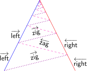
(b) Accumulating with $4$ speeds.

Figure 7: Meta-signals, rules and an accumulation of the machine $\mathfrak{M}_{4}$.

This machine allows to generate an accumulation, when started from a well-chosen but very simple initial configuration:

Lemma 6.

The signal machine $\mathfrak{M}_{4}$ generates an accumulation at coordinates $(0,2)$ when started from $c_{0}=\{\ \overrightarrow{\textsf{\sf{left}}}@{-1},\ \overrightarrow{\textsf{\sf{zig}}}@{-1},\ \overleftarrow{\textsf{\sf{right}}}@{1}\ \}$,

Proof.

We consider the sequence $(C_{n})_{n\in\mathbb{N}}$ of consecutive collisions on the diagram generated by $\mathfrak{M}_{4}$ from the configuration $c_{0}$ and we note $(x_{n},t_{n})$ the corresponding (spatial and temporal) coordinates. We also define $\delta_{n}$ as the duration between two consecutive collisions $C_{n}$ and $C_{n+1}$, i.e., $\delta_{n}=t_{n+1}-t_{n}\enspace$.

We compute coordinates of each $C_{n}$ and show that the sequence of collisions happening during the computation is an alternation of the two collision rules defined previously, i.e., for all $n\geq 0$ we have:

$$C_{n}=\begin{cases}\ \{\overrightarrow{\textsf{\sf{zig}}},\overleftarrow{\textsf{\sf{right}}}\}\rightarrow\{\overleftarrow{\textsf{\sf{zag}}},\overleftarrow{\textsf{\sf{right}}}\}&\text{ if }n\text{ is odd}\textit{ (right-bounce)}\\[3.00003pt] \ \{\overrightarrow{\textsf{\sf{left}}},\overleftarrow{\textsf{\sf{zag}}}\}\rightarrow\{\overrightarrow{\textsf{\sf{left}}},\overrightarrow{\textsf{\sf{zig}}}\}&\text{ if }n\text{ is even}\textit{ (left-bounce)}\end{cases}\enspace.$$

We suppose by convention that $C_{0}$ of coordinate $(x_{0},t_{0})$ is so that $x_{0}=-1$ (initial positions of $\overrightarrow{\textsf{\sf{left}}}$ and $\overrightarrow{\textsf{\sf{zig}}}$) and $t_{0}=0$, and that $C_{0}$ is a right-bounce. This can be interpreted as a collision happening in the initial configuration and produces the same configuration as $c_{0}$. Note that positions of $\overrightarrow{\textsf{\sf{left}}}$ and $\overleftarrow{\textsf{\sf{right}}}$ are always opposite since they have opposite speeds and they are initially disposed symetrically to $0$ (collision rules ensure that they keep their motions after each collision).

Suppose that a configuration at a time $t_{n}$ is $c_{t_{n}}=\{\ \overrightarrow{\textsf{\sf{left}}}@{x_{n}},\ \overrightarrow{\textsf{\sf{zig}}}@{x_{n}},\ \overleftarrow{\textsf{\sf{right}}}@{-x_{n}}\ \}$. Any configuration coming from a left-bounce collision $C_{n}$ of coordinates $(x_{n},t_{n})$ verifies this displaying of signals. In particular, this is the case for the initial configuration $c_{0}$ with $x_{0}=-1$. It is clear from the disposition of signals that the next collision $C_{n+1}$ to happen is a right-bounce i.e. $\{\overrightarrow{\textsf{\sf{zig}}},\ \overleftarrow{\textsf{\sf{right}}}\}\rightarrow\{\overleftarrow{\textsf{\sf{zag}}},\ \overleftarrow{\textsf{\sf{right}}}\}$ because $\overrightarrow{\textsf{\sf{zig}}}$ (of speed $4$) is moving right and is located on the left of $\overleftarrow{\textsf{\sf{right}}}$ (of speed $-\frac{1}{2}$) which is moving left. Signals $\overrightarrow{\textsf{\sf{left}}}$ and $\overrightarrow{\textsf{\sf{zig}}}$ cannot collide since $\overrightarrow{\textsf{\sf{left}}}$ is on the left of $\overrightarrow{\textsf{\sf{zig}}}$, which moves to the right faster than $\overrightarrow{\textsf{\sf{left}}}$. The collision between $\overrightarrow{\textsf{\sf{zig}}}$ and $\overleftarrow{\textsf{\sf{right}}}$ is deduced from the respective dynamics, and its coordinates $(x,t$) satisfy: $\begin{cases}x=4\cdot(t-t_{n})+x_{n}&\text{(motion of $\overrightarrow{\textsf{\sf{zig}}}$)}\\ x=-\frac{1}{2}\cdot(t-t_{n})-x_{n}&\text{(motion of $\overleftarrow{\textsf{\sf{right}}}$)}\end{cases}\enspace.$

At the time $t_{n+1}$, the next collision happens and both signals $\overrightarrow{\textsf{\sf{zig}}}$ and $\overleftarrow{\textsf{\sf{right}}}$ occupy the same position after the duration $\delta_{n}=t_{n+1}-t_{n}$ which satisfies $4\cdot\delta_{n}+x_{n}=-\frac{1}{2}\cdot\delta_{n}-x_{n}$. The delay $\delta_{n}$ and the position $x_{n+1}$ are given by:

$$\delta_{n}=-\frac{4}{9}\cdot x_{n}\quad\text{ and }\quad x_{n+1}=-\frac{7}{9}\cdot x_{n}\enspace.$$ (1)

Since incoming signals of the collision $C_{n+1}$ have been replaced by outcoming signals, the configuration at the time $t_{n+1}$ is given by: $c_{t_{n+1}}=\{\ \overrightarrow{\textsf{\sf{left}}}@{-x_{n+1}},\ \overleftarrow{\textsf{\sf{zag}}}@{x_{n+1}},\ \overleftarrow{\textsf{\sf{right}}}@{x_{n+1}}\ \}$.

For the symmetric case, when $c_{t_{n}}=\{\ \overrightarrow{\textsf{\sf{left}}}@{-x_{n}},\ \overrightarrow{\textsf{\sf{zig}}}@{x_{n}},\ \overleftarrow{\textsf{\sf{right}}}@{x_{n}}\ \}$ and $C_{n}$ is a right-bounce, the next collision $C_{n+1}$ is a left-bounce and we obtain by the same way its position $x_{n+1}$ and the duration $\delta_{n}$ between $C_{n}$ and $C_{n+1}$:

$$\delta_{n}=\frac{4}{9}\cdot x_{n}\quad\text{and}\quad x_{n+1}=-\frac{7}{9}\cdot x_{n}$$ (2)

So, starting from the initial configuration $c_{0}$ and applying successively the previous computations for each configuration after each collision, we obtain an alternation of right-bounces and left-bounces (starting with a right-bounce). By Eq. (1) and Eq. (2), sequences $(x_{n})_{n\in\mathbb{N}}$ and $(\delta_{n})_{n\in\mathbb{N}}$ satisfy:

$$\left\{\begin{array}[]{l@{}}x_{0}=-1\ ;\ x_{n+1}=-\frac{7}{9}\cdot x_{n}\\[5.0pt] \delta_{n}\ =\ \left(-1\right)^{n+1}\cdot\frac{4}{9}\cdot x_{n}\end{array}\right.\text{ which gives }\forall n\in\mathbb{N},\left\{\begin{array}[]{l@{}}x_{n}=(-1)^{n+1}\cdot\left(\frac{7}{9}\right)^{n}\\[5.0pt] \delta_{n}=\frac{4}{9}\cdot\left(\frac{7}{9}\right)^{n}\end{array}\right.\enspace.$$

Finally, from the relation $t_{n+1}=t_{n}+\delta_{n}$ and $t_{0}=0$, we obtain for all $n\in\mathbb{N}\,$:

$$t_{n+1}\ =\ \sum\limits_{i=0}^{n}\delta_{i}\ =\ \sum\limits_{i=0}^{n}\frac{4}{9}\times\left(\frac{7}{9}\right)^{i}\ =\ \frac{4}{9}\times\sum\limits_{i=1}^{n}\left(\frac{7}{9}\right)^{i}\enspace.$$

The sequence $(t_{n})_{n\in\mathbb{N}}$ is infinite, strictly increasing and positive. It admits a limit which is given by the sum of the geometrical sequence of ratio $\frac{7}{9}~{}<~{}1\,$:

$$\lim\limits_{n\to\infty}t_{n}=\ \frac{4}{9}\times\lim\limits_{n\to\infty}\sum\limits_{i=0}^{n}\left(\frac{7}{9}\right)^{i}\ =\ \frac{4}{9}\times\frac{1}{1-\frac{7}{9}}\ =\ 2\enspace.$$

The sequence $(x_{n})_{n\in\mathbb{N}}$ of spatial positions also admits a limit:

$$\lim\limits_{n\to\infty}x_{n}\ =\ \lim\limits_{n\to\infty}\left|\left(-1\right)^{n}\cdot\left(\frac{7}{9}\right)^{n}\right|\ =\ \lim\limits_{n\to\infty}\left(\frac{7}{9}\right)^{n}\ =\ 0\enspace.$$

So the machine $\mathfrak{M}_{4}$ runned from initial configuration $c_{0}$ produces a sequence of successive collisions at coordinates $(x_{n},t_{n})$ satisfying $\lim\limits_{n\to\infty}(x_{n},t_{n})=(0,2)$. According to Def. 9 and Lem. 5, we have $c_{\tilde{t}}(0)=c_{2}(0)=\text{\char 90}$, i.e., the point $(0,2)$ is an accumulation. ∎

Example of the machine $\mathfrak{M}_{4}$ gives us the following:

Corollary 2.

Accumulations can be generated by $4$-speed signal machines.

Remark.  As soon as a signal machine contains four meta-signals, all having distinct speeds so that two of them can bounce alternatively between the two other ones, then this signal machine can generate accumulations in kind of the one described above (with proper initial positions for three of these four meta-signals). This suggests that the ability to accumulate is not so rare for signal machines having a sufficient number of speed values.

3.2 Case of 2 speeds

We now consider the case of $2$-speed machines, and prove that no matter what are these two speeds, no accumulation can occur in such machine.

Reduction to a normalized machine

Let $\mathfrak{M}^{a,b}=(\mathcal{M},\mathcal{S},\mathcal{R})$ be a signal machine with meta-signals having only two distinct speeds $a$, $b$ $\in\mathbb{R}$ with $a<b$. We define a function $g:\mathbb{R}\to\mathbb{R}$ by $g(x)=\frac{x}{b-a}-\frac{a}{b-a}$. We have $g(a)=0$ and $g(b)=1$ (in fact, $g$ is the function $f$ defined in Subsect. 2.3, with $c=0$ and $d=1$).

We normalize the machine $\mathfrak{M}^{a,b}$ into the machine $\mathfrak{M}^{0,1}=(\mathcal{M},\mathcal{S}^{\prime},\mathcal{R})$ where $\mathcal{S}^{\prime}=g\circ\mathcal{S}$. Speed values of $\mathfrak{M}^{0,1}$ are $0$ and $1$. As $g$ is an affine function with a strictly positive ratio (because $a<b$) and $\mathfrak{M}^{0,1}=\mathfrak{M}_{g}^{a,b}$, we obtain by Lem. 1 that $\mathfrak{M}^{0,1}$ produces space-time diagrams equivalent to the ones generated by $\mathfrak{M}^{a,b}$. In particular, if $\mathfrak{M}^{a,b}$ produces accumulations, then $\mathfrak{M}^{0,1}$ will also produce accumulations.

Accumulating is impossible with only 2 speeds

We can now give the proof that no signal machine having only two distinct speeds can produce an accumulation. By Lem. 1 and Coro. 1, it is enough to prove that no accumulation can occur in any support diagrams of the signal machine having only two meta-signals, one of speed $0$ and one of speed $1$.

Hence we can consider, without any loss of generality, a signal machine $\mathfrak{M}_{2}$ having only two meta-signals: S of speed $0$ and $\overrightarrow{\textsf{\sf{R}}}$ of speed $1$. As $\mathfrak{M}_{2}$ contains only two meta-signals, there is only one collision rule to be defined in the machine and to have $\mathfrak{M}_{2}$ to be a support machine, we necessarily have: $\{\overrightarrow{\textsf{\sf{R}}},\textsf{\sf{S}}\}\rightarrow\{\textsf{\sf{S}},\overrightarrow{\textsf{\sf{R}}}\}\enspace.$

Lemma 7.

Let $c_{0}$ an initial configuration for $\mathfrak{M}_{2}$. Let $i$ be the number of signals $\overrightarrow{\textsf{\sf{R}}}$ in $c_{0}$ and $j$ the number of signals S. Then the diagram generated by $\mathfrak{M}_{2}$ starting from $c_{0}$ contains at most $i\times j$ collisions.

Proof.

Any finite initial configuration (see e.g. Fig. 8(a)) can be rearranged in an initial configuration that maximize the number of possible collisions. Indeed, the maximum number of collisions is obtained if each signal $\overrightarrow{\textsf{\sf{R}}}$ collides with each signal S. This is possible only if each $\overrightarrow{\textsf{\sf{R}}}$ is initially disposed at the left of each signal S. So for computing the exact upper-bound of the number of collisions, we consider an initial configuration similar to the one displayed Fig. 8(b), i.e., the position of each signal $\overrightarrow{\textsf{\sf{R}}}$ is strictly lower than the positions of any signal S.

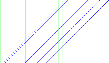
(a) Diagram from a random initial configuration.

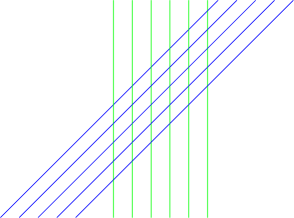
(b) Bounding the number of collisions.

Figure 8: Diagrams of the machine $\mathfrak{M}_{2}$.

Since the unique collision rule outputs all incoming signals, each signal $\overrightarrow{\textsf{\sf{R}}}$ is not annihilated after colliding the first (i.e., the left-most) signal S encountered but $\overrightarrow{\textsf{\sf{R}}}$ continues and collides with all the signals S, that is the $j$ signals S present in the initial configuration. After colliding the last (i.e., the right-most) signal S, $\overrightarrow{\textsf{\sf{R}}}$ propagates to the right ad infinitum and does not collide again.

Thus each signal $\overrightarrow{\textsf{\sf{R}}}$ generates $j$ collisions. As the number of signals $\overrightarrow{\textsf{\sf{R}}}$ is $i$ and as each one collides with all signals S, the total number of collisions is $i\times j\enspace$. ∎

Remark.  Given $n$ signals in the initial configuration, the maximum number of collisions $i\times j$ is obtained by taking $i=\lfloor\frac{n}{2}\rfloor$ signals $\overrightarrow{\textsf{\sf{R}}}$ and $j=n-i$ signals S in the initial configuration so that each signal $\overrightarrow{\textsf{\sf{R}}}$ is initially located at the left of any signal S.

Proposition 1.

Accumulations cannot be generated by a signal machine (rational-like or not) having only two distinct speeds and starting from a finite configuration.

Proof.

As explained before, any $2$-speed machine $\mathfrak{M}$ can be normalized into a $2$-speed machine $\mathfrak{M}^{0,1}$ (with speeds $0$ and $1$). This machine has for support machine the machine $\mathfrak{M}_{2}$. By Lem. 7, $\mathfrak{M}_{2}$ runned from a finite initial configuration can produce at most a finite number of collisions, and as a necessary (but no sufficient) condition for having accumulation is to contain an infinite number of signals/collisions in the diagram, it follows that $\mathfrak{M}_{2}$ cannot generate accumulation. Lemma 1 and Coro. 1 imply that neither $\mathfrak{M}^{0,1}$ nor $\mathfrak{M}$ can produce accumulation. We conclude that no accumulation can be generated by any $2$-speed machine. ∎

It has to be underlined that in the case of two signals, the rationality of speeds or initial positions doesn’t play any role (the normalization of speeds $a$ and $b$ to speeds $0$ and $1$ can be done for any numbers $a$ and $b$, rationals or not, and initial positions do not need to be rational in the proof of Lem. 7). But the hypothesis of finitude of the initial configuration is necessary.

Obviously, it is always possible to create an accumulation with only two speeds if we consider infinite initial configurations: it is enough to place stationary signals such that a (static) accumulation is present in the initial configuration e.g. an accumulation in $0$ by placing a stationary signal at each position $-1/n$ (this infinite initial configuration remains rational). Then a right signal $\overrightarrow{\textsf{\sf{R}}}$ (having speed $1$) at position $-2$ will collide all stationary signals before time $2$, producing a (dynamic) accumulation at coordinates $(0,2)$, as illustrated by Fig. 9 (wihere the rule used is $\{\overrightarrow{\textsf{\sf{R}}},\textsf{\sf{S}}\}\rightarrow\{\overrightarrow{\textsf{\sf{R}}}\}$).

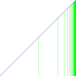
Figure 9: Accumulation with $2$ speeds and an infinite initial configuration.

4 Case of 3 speeds

We showed in the previous section that building an accumulation is easy with $4$ speeds, whereas it is impossible with only $2$ distinct speeds. In this section, we study the border case —accumulations with $3$ speeds— and we show that two sub-cases have to be distinguished: one treating rational-like signal machines and the other one dealing with fully irrational machines. The main result is that a $3$-speed machine $\mathfrak{M}$could produce accumulations if and only if $\mathfrak{M}$ involves an irrational ratio (there exists an irrational ratio either between two speed values or between two initial positions). First, we exhibate a simple signal machine and an irrational configuration from which the machine produces an accumulation: this is done by implementing a geometrical version of Euclid’s algorithm, and by executing an infinite run of this algorithm. We also provide, with a slight modification of this machine, an example of accumulation from a rational initial configuration and with $3$ speeds, one of them having an irrational value. In a second part, we prove that any diagram of a $3$-speed rational machine is included in some regular diagrams called meshes; none of these meshes contain accumulation, and so neither does any diagram of a $3$-speed rational machine.

4.1 Case of irrational machines

Euclid’s algorithm is based on the computation of the remainder of two numbers, and to implement it on signal machines, we use the geometrical computation of the modulo of two reals values, as mentionned in Subsect. 2.2: starting with a configuration that encodes some values $a$ and $b$, we can obtain after some number of collisions the value of $a\bmod b$, also encoded between two vertical signals. We describe below how we can compute the greatest common divisor of two values by iterating the process of a modulo computation, and we use the properties of Euclid’s algorithm to build an accumulation.

A $3$-speed machine implementing Euclid’s algorithm

To provide an accumulation with three speeds, we define a simple $3$-speed machine, $\mathfrak{M}_{gcd}$. This machine computes the greates common divisor of two values by implementing and following the steps of Euclid’s algorithm.

Euclid’s algorithm, starting from two real numbers $a$ and $b$ ($b\leq a$), defines the sequences $(a_{n})_{n\in\mathbb{N}}$ and $(b_{n})_{n\in\mathbb{N}}$ by the following recursion:

$\begin{cases}a_{0}=a\\ b_{0}=b\end{cases}$  et

$\begin{cases}a_{n+1}=b_{n}\\ b_{n+1}=a_{n}\bmod b_{n}\end{cases}\enspace.$

This recursion also provides the sequence $(r_{n})_{n\in\mathbb{N}}$ of remainders of the successive euclidean divisions, given by $r_{n}=a_{n}\bmod b_{n}$, and the sequence $(q_{n})_{n\in\mathbb{N}}$ of the quotients, defined by $q_{n}=a_{b}/b_{n}$. If the sequence $(a_{n})_{n\in\mathbb{N}}$ becomes equal to zero from one rank, then the greatest $a_{n}$ so that $a_{n}\neq 0$ is the greatest common divisor ($\gcd$) of $a$ and $b$. Otherwise, the $\gcd$ of $a$ and $b$ is not defined.

This algorithm can be geometrically implemented by a $3$-speed machine composed by seven meta-signals (three of speed $0$, two of speed $1$ and two of speed $-1$) and eight rules. We give in Fig. 10(a) the definition of such a machine $\mathfrak{M}_{gcd}$, and a run example is displayed in Fig. 10(b), which corresponds to the computation of $\gcd(8,3)$ (coded by the distance between the two remaining signals w₀ at the very top of the diagram).

Meta-signal Speed $\overrightarrow{\textsf{\sf{zig}}}$, $\overrightarrow{\textsf{\sf{ZIG}}}$ $1$ w0, wa, wb $0$ $\overleftarrow{\textsf{\sf{zag}}}$, $\overleftarrow{\textsf{\sf{ZAG}}}$ $-1$

Collision rules   (1) { $\overrightarrow{\textsf{\sf{zig}}}$, wb } $\rightarrow$ { $\overleftarrow{\textsf{\sf{zag}}}$, wb, $\overrightarrow{\textsf{\sf{ZIG}}}$ }   (2) { w0, $\overleftarrow{\textsf{\sf{zag}}}$ } $\rightarrow$ { w0, $\overrightarrow{\textsf{\sf{zig}}}$ }   (3) { wa, $\overrightarrow{\textsf{\sf{ZIG}}}$ } $\rightarrow$ { $\overleftarrow{\textsf{\sf{ZAG}}}$ }   (4) { wb, $\overleftarrow{\textsf{\sf{ZAG}}}$ } $\rightarrow$ { $\overleftarrow{\textsf{\sf{ZAG}}}$, wa }   (5) { $\overrightarrow{\textsf{\sf{zig}}}$, $\overleftarrow{\textsf{\sf{ZAG}}}$ } $\rightarrow$ { $\overleftarrow{\textsf{\sf{zag}}}$, wb }   (6) { $\overrightarrow{\textsf{\sf{ZIG}}}$, $\overleftarrow{\textsf{\sf{ZAG}}}$ } $\rightarrow$ { $\overleftarrow{\textsf{\sf{ZAG}}}$ }   (7) { $\overrightarrow{\textsf{\sf{zig}}}$, wb, $\overleftarrow{\textsf{\sf{ZAG}}}$ } $\rightarrow$ { $\overleftarrow{\textsf{\sf{ZAG}}}$, w0 }   (8) { w0, $\overleftarrow{\textsf{\sf{ZAG}}}$ } $\rightarrow$ { w0 }

(a) Meta-signals and rules of $\mathfrak{M}_{gcd}$.

(b) A run of $\mathfrak{M}_{gcd}$ computing $\gcd(8,3)=1$.

Figure 10: Meta-signals, rules and a run of the machine $\mathfrak{M}_{gcd}$.

As done in Subsect. 2.2, the stationary meta-signals (w₀, w_a and w_b) are used to encode two real numbers: the real value $a$ (resp. $b$) is the distance between signals w₀ and w_a (resp. w_b). In our geometrical version, the step $a_{n+1}=b_{n}$ is implemented by the rule (10(a)) of Fig. 10(a) and the step $b_{n+1}=a_{n}\bmod b_{n}$ by the rule (10(a)). Rules (10(a)) and (10(a)) correspond to the two last collisions when the process halts, as shown in the top of Fig. 10(b).

We denote by $c^{a,b}$ ($a>b$) the configuration using only four signals (including one non-stationary signal) and respecting the previous encoding of the values between the stationary signals: $c^{a,b}=\{\ \textsf{\sf{w${}_{0}$}}@{0},\ \overrightarrow{\textsf{\sf{zig}}}@{0},\ \textsf{\sf{w${}_{b}$}}@{b},\ \textsf{\sf{w${}_{a}$}}@{a}\ \}$. The distance between w₀ and w_a (resp. w_b) is indeed $a$ (resp. $b$).

Remark.  Starting from a configuration having two stationary signals and one moving (say to the right) from the first stationary signal to the second the time of a back-and-forth depends on the distance $d$ between the stationary signals and the speeds of the signals making the bounce. This is the cases here with a configuration $c^{a,b}$, where $\overrightarrow{\textsf{\sf{zig}}}$ and $\overleftarrow{\textsf{\sf{zag}}}$ will make a back-and-forth between w₀ and w_b (resp. $\overrightarrow{\textsf{\sf{ZIG}}}$ and $\overleftarrow{\textsf{\sf{ZAG}}}$ making a back-and-forth between w₀ and w_a). This time is equal to the sum of the time for the right and left signal to reach the opposite wall and is given by $(1+1)\cdot d=2d$ (remember the speeds are $1$ and $-1$). Note that in the general case of non-null speeds $\nu_{1}$ and $-\nu_{2}$, the time of a back-and-forth is given by $\frac{1}{\nu_{1}}d+\frac{1}{\nu_{2}}d=\left(\frac{1}{\nu_{1}}+\frac{1}{\nu_{2}}\right)\cdot d=\uptau\cdot d$, where $\uptau=\frac{1}{\nu_{1}}+\frac{1}{\nu_{2}}$ is the time a of unitary back-and-forth.

Let us describe briefly the evolution of $\mathfrak{M}_{gcd}$ on such a configuration. Consider first the case $a\bmod b\neq 0$. After signals $\overrightarrow{\textsf{\sf{ZIG}}}$ (firstly $\overrightarrow{\textsf{\sf{zig}}}$) and $\overleftarrow{\textsf{\sf{ZAG}}}$ (firstly $\overleftarrow{\textsf{\sf{zag}}}$) have completed the back-and-forth between w₀ and w_a, that is after the duration $\uptau a$ according to the previous remark, the configuration has the same form than the initial configuration $c^{a,b}$, but now with the two walls w_a and w_b that have been moved to new positions. Indeed, with respect to the rules, the initial w_a has now disappeared, the initial w_b has be turned into w_a by $\overleftarrow{\textsf{\sf{ZAG}}}$ and the collision between $\overrightarrow{\textsf{\sf{zig}}}$ (which was bouncing between signals w₀ and w_b, being turned alternatively into $\overrightarrow{\textsf{\sf{zig}}}$ and $\overleftarrow{\textsf{\sf{zag}}}$) and $\overleftarrow{\textsf{\sf{ZAG}}}$ has created a new w_b, the first wall w₀ remaining unchanged. This process is displayed in Fig. 11(a).

If we call $a^{\prime}$ (resp. $b^{\prime}$) the distance between w₀ and the new w_a (resp. w_b) as illustrated by Fig. 11(a), the new configuration at time $2a$ is $c^{a^{\prime},b^{\prime}}=\{\textsf{\sf{w${}_{0}$}}@0,\ \overrightarrow{\textsf{\sf{zig}}}@0,\ \textsf{\sf{w${}_{b}$}}@b^{\prime},\ \textsf{\sf{w${}_{a}$}}@a^{\prime}\}$. We have: $2a=k\cdot 2b+2r$, where $k\in\mathbb{N}$ and $0\leq 2r<2b$ (by definition of $2r$ which is defined from the wall appearing between walls encoding $b$). So $2r$ is the remainder in the Euclidean division of $2a$ by $2b$: $2r=2a\bmod 2b$, that is $r=a\bmod b$. We have $a^{\prime}=b$ and $b^{\prime}=r=a\bmod b\neq 0$. Finally, from the configuration $c^{a,b}$, we obtain after the duration $2a$ the configuration $c^{a^{\prime},b^{\prime}}=c^{b,a\bmod b}$.

For the case $r=0$ (i.e. when $b$ divides $a$), the collision involving $\overleftarrow{\textsf{\sf{ZAG}}}$ and w_b also involves $\overrightarrow{\textsf{\sf{zig}}}$ and the rule (10(a)) is applied. The next collision necessarily happens between w₀ and $\overleftarrow{\textsf{\sf{ZAG}}}$, and after the application of the rule (10(a)) only two signals w₀, spaced by the distance $b$ remains on the space.

By iterating the process and starting with $a=a_{0}$ and $b=b_{0}$, we can define the sequences $(a_{n})_{n\in\mathbb{N}}$ and $(b_{n})_{n\in\mathbb{N}}$ by identifying at each step of the process the distances $a,a^{\prime},b$ and $b^{\prime}$ respectively with the values $a_{n},a_{n+1},b_{n}$ and $b_{n+1}$. The sequences thus obtained correspond to the ones defined by the double recursion of Euclid’s algorithm with initial conditions $a_{0}=a$ and $b_{0}=b$: we have $a_{n+1}=b_{n}$ and $b_{n+1}=a_{n}\bmod b_{n}$. If for some $n_{0}$, $a_{n_{0}}$ is a multiple of $b_{n_{0}}$, it means that $\overleftarrow{\textsf{\sf{ZAG}}}$ and w_b will also collide with $\overrightarrow{\textsf{\sf{zig}}}$ into a triple collision. As mentionned above, rules (10(a)) and (10(a)) bring the process to a halt, leaving two signals w₀: the distance between them is the last non-null remainder and so, it is the $\gcd$ of $a_{0}$ and $b_{0}$.

(a) A step of the geometrical Euclid’s algorithm.

(b) An accumulation with $3$ speeds.

Figure 11: Achieving an accumulation with the machine $\mathfrak{M}_{gcd}$.

Non-termination of Euclid’s algorithm

To provide an accumulation, an infinite number of collisions should take place in a finite time, and so this process should be infinite. This means that we need to execute Euclid’s algorithm on some values $a$, and $b$ such that it doesn’t end. To achieve this, it is enough to use two incommensurate reals i.e., two reals such that their ratio is irrational. Indeed, it is know from [Hardy and Wright, 1960, Th. 161, p. 136] that:

$$\text{{\em Euclid's algorithm halts on inputs $a$ and $b$}}\ \ \Longleftrightarrow\ \ \frac{a}{b}\in\mathbb{Q}\enspace.$$

To obtain an infinite run, we set the values $a=\varphi$ and $b=1$, where $\varphi=\frac{1+\sqrt{5}}{2}$ is the golden number. The generated diagram is given by Fig. 11(b), and the corresponding initial configuration is $c_{0}^{\varphi,1}=\{\textsf{\sf{w${}_{0}$}}@0,\ \overrightarrow{\textsf{\sf{zig}}}@0,\ \textsf{\sf{w${}_{b}$}}@1,\ \textsf{\sf{w${}_{a}$}}@\varphi\}$.

Executed on these inputs, the algorithm doesn’t terminate because $\frac{a}{b}=\varphi$ is irrational, and it produces a sequence $(r_{n})_{n\in\mathbb{N}}$ of remainders wich is striclty positive and decreasing (by definition of the Euclidean division). Also, as $\varphi$ satisfies $\varphi=1+\frac{1}{\varphi}$, the developement of $\varphi$ into a continued fraction is:

$$\varphi=1+\frac{1}{1+\frac{1}{1+\frac{1}{\ldots}}}$$

and it provides that $q_{n}=1$ for all $n$ (see [Hardy and Wright, 1960, p. 134] for more details on the link between continued fraction and Euclid’s algorithm).

Convergence of sum of $a_{n}$ and limit of the sequence of collision times

We prove here that the diagram of Fig. 11(b) indeed contains an accumulation. Starting from $a_{0}=a$, $b_{0}=b$, by using the definition of $a_{n+1}=b_{n}$ and $b_{n+1}=r_{n}$ and the relation $a_{n}=b_{n}\cdot q_{n}+r_{n}$ for all $n\in\mathbb{N}$, we can prove in the general case that for all $n$ we have $a_{n+2}\leq\frac{1}{2}a_{n}$.
Indeed, we have:

$$a_{n} =b_{n}\cdot q_{n}+r_{n}$$

$$=a_{n+1}\cdot q_{n}+b_{n+1} \text{ since }a_{n+1}=b_{n}\text{ and }b_{n+1}=r_{n}\,,$$

$$=(b_{n+1}\cdot q_{n+1}+r_{n+1})\cdot q_{n}+b_{n+1}$$

$$=b_{n+1}(1+q_{n+1}\cdot q_{n})+r_{n+1}\cdot q_{n}$$

$$=a_{n+2}(1+q_{n+1}\cdot q_{n})+r_{n+1}\cdot q_{n} \text{ since }a_{n+2}=b_{n+1}\,,$$

$$\geq 2a_{n+2}+r_{n+1} \text{ because }\forall n\ q_{n}\geq 1\,.$$

We know that starting from $a_{0}=\varphi$ and $b_{0}=1$, since the ratio $a_{0}/b_{0}$ is irrational, the algorithm doesn’t terminate and so we have $r_{n}>0$ for all $n$. We also have for all $n$ $q_{n}=1$. So in the case of inputs $\varphi$ and $1$, the previous inequality simply becomes:

$$a_{n+2}<\frac{1}{2}a_{n}\enspace.$$

By a simple induction on $n$, we obtain $\forall n\geq 1$, $a_{2n}<\frac{1}{2^{n}}a_{0}$ and $a_{2n+1}<\frac{1}{2^{n}}a_{1}$. Finally:

$$\sum\limits_{i=0}^{n}a_{i} =\ \sum\limits_{i=0}^{\lfloor n/2\rfloor}a_{2i}+\sum\limits_{i=0}^{\lfloor n/2\rfloor}a_{2i+1}$$

$$<\ \sum\limits_{i=0}^{\lfloor n/2\rfloor}\frac{1}{2^{i}}\cdot a_{0}+\sum\limits_{i=0}^{\lfloor n/2\rfloor}\frac{1}{2^{i}}\cdot a_{1}$$

$$<\ a_{0}\cdot\sum\limits_{i=0}^{\lfloor n/2\rfloor}\frac{1}{2^{i}}+a_{1}\cdot\sum\limits_{i=0}^{\lfloor n/2\rfloor}\frac{1}{2^{i}}$$

and when $n\to\infty$, we get for the values $a_{0}=\varphi$ and $a_{1}=b_{0}=1$:

$$\lim\limits_{n\to\infty}\sum\limits_{i=0}^{n}a_{i} <\ 2\cdot(\varphi+1)$$

Since the series $\Sigma a_{i}$ is upper-bounded by $2\cdot(\varphi+1)$, and has positive terms, the infinite sum $\sum\limits_{i=0}^{\infty}a_{i}$ converges to a finite limit.

Each time a recursive step of the algorithm starts, at least one collision has occured (in fact at least $3$), and so each duration $2a_{i}$ contains at least one collision (remember that the value $2$ is the coefficient of a back-and-forth duration, and it only depends on the speeds, which values are here $1$ and $-1$). More precisely, for all $n\in\mathbb{N}$, there is a collision occuring at coordinates $(0,2\cdot\sum\limits_{i=0}^{n}a_{i})$, and between time $2\cdot\sum\limits_{i=0}^{n}a_{i}$ and $2\cdot\sum\limits_{i=0}^{n+1}a_{i}$, there is only a finite number of collisions.

The total sum of these durations is given by $\tilde{t}=\sum\limits_{i=0}^{\infty}2a_{i}$ and corresponds to the total height of the construction. As we showed previsouly, the infinite sum $\sum\limits_{i=0}^{\infty}a_{i}$ is bounded by $2\cdot(\varphi+1)$ and so $\tilde{t}$ is upper-bounded by $4\cdot(\varphi+1)$. We can conclude that before the finite time $\tilde{t}$, there is an infinite number of collisions, because there is at least one collision occuring at each time $t=2\cdot\sum\limits_{i=0}^{n}a_{i}<\tilde{t}$. This implies by definition of the sequence of collisions $(C_{n})_{n\in\mathbb{N}}$ (Def. 9), that the sequence of collision times is converging to $\tilde{t}$. In the general case, $\tilde{t}$ is bounded by $2\uptau\cdot(a_{0}+b_{0})$, where $\uptau=\frac{1}{\nu_{1}}+\frac{1}{\nu_{2}}$ (for non-null speeds $\nu_{1}$ and $\nu_{2}$) and $a_{0}$ and $b_{0}$ are positive real numbers.

By Lem. 5, the diagram of $\mathfrak{M}_{gcd}$ started on the initial configuration $c_{0}^{1,\varphi}$ contains an accumulation happening at coordinates $(0,\tilde{t})$ i.e. it satisfies $c_{\tilde{t}}(0)=\text{\char 90}$. More generally, by using the property that Euclid’s algorithm halts on inputs $a$ and $b$ if and only if $\frac{a}{b}$ is irrational, we obtain the following:

Lemma 8.

The machine $\mathfrak{M}_{gcd}$ produces an accumulation when executed from any initial configuration $c_{0}^{a,b}$ satisfying $\frac{a}{b}\notin\mathbb{Q}$.

Remark.  According to this lemma, $\varphi$ can be replaced by any other irrational value $x$ (greater than $1$): the machine $\mathfrak{M}_{gcd}$ run from $c_{0}^{1,x}$ will also produce an accumulation. Here, $\varphi$ has been chosen because of the regularity of the resulted diagram, coming from the fact that Euclid’s algorithm started on $\varphi$ and $1$ satisfies $q_{n}=1$ for all $n$.

We can also provide an accumulation by using $\widehat{\mathfrak{M}_{3}^{-1,0,1}}$, the support machine of $\mathfrak{M}_{gcd}$, using only three meta-signals, and by running it on $\widehat{c_{0}^{1,\varphi}}$, the support configuration of $c_{0}^{1,\varphi}$. We obtain the diagram of Fig. 12(a), in which an accumulation happens at position $x=1$ and strictly before the time $\tilde{t}$ computed previsouly. Another example is displayed by Fig. 12(b). The fact that these support diagrams contain an accumulation directly follow by Coro. 1 and Lem. 8.

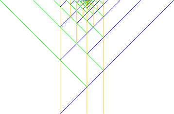
(a) Support diagram for $c_{0}^{1,\varphi}$.

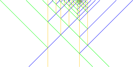
(b) Another example.

Figure 12: Examples of supports diagrams for $\mathfrak{M}_{gcd}$ with an accumulation.

Accumulation with an irrational speed and a rational initial configuration

We can also provide an accumulation starting with a rational initial configuration, but with a signal machine including meta-signals of irrational speed, which can be used to create an irrational distance.

To achieve this, we start from the machine $\mathfrak{M}_{gcd}$ in which all speeds $1$ are replaced by speeds $\varphi\in\mathbb{R}\smallsetminus\mathbb{Q}$. This new machine $\mathfrak{M}_{gcd}^{\varphi}$ is given in Fig. 13(a). We can easily set an initial rational configuration so that, by using the fact that $\frac{-1}{\varphi}$ (the ratio between the two non-zero speeds) is irrational, we obtain after two collisions an irrational configuration wich can be used to run Euclid’s algorithm. We use a new meta-signal, $\overrightarrow{\textsf{\sf{start}}}$, of speed $\varphi$, and the rule $\{\overrightarrow{\textsf{\sf{start}}},\ \overleftarrow{\textsf{\sf{zag}}}\}\rightarrow\{\overleftarrow{\textsf{\sf{zag}}},\ \textsf{\sf{w${}_{b}$}}\}$ to set a stationary signal w_b at an irrational position. Indeed, as illustrated by Fig. 13(b), if we start from the rational configuration $c_{0}=\{\textsf{\sf{w${}_{0}$}}@0,\ \overrightarrow{\textsf{\sf{start}}}@0,\ \overleftarrow{\textsf{\sf{zag}}}@1,\ \textsf{\sf{w${}_{a}$}}@1\}$, a simple computation shows that the first collision happens at the position $x=\frac{1}{1+\varphi}=\frac{1}{\varphi}=\varphi-1$ and that the configuration at time $1$ has the form $c_{1}^{1,\varphi-1}=\{\textsf{\sf{w${}_{0}$}}@0,\ \overrightarrow{\textsf{\sf{zig}}}@0,\ \textsf{\sf{w${}_{b}$}}@\varphi-1,\ \textsf{\sf{w${}_{a}$}}@1\}$, which is the required form to start an infinite execution of the Euclid’s algorithm explained previously. In this initialization, the irrational speeds is used to create an irrational distance from a rational initial configuration. After the initialization, the process never halts because the ratio $\frac{1}{\varphi-1}=\varphi$ is irrational, and because the rules of $\mathfrak{M}_{gcd}^{\varphi}$ (except the one involving $\overrightarrow{\textsf{\sf{start}}}$) are the same than $\mathfrak{M}_{gcd}$. The sequence $(a_{n})_{n\in\mathbb{N}}$ is the same than the previous example, but shifted by one step because of the initialization which sets the first values at $a_{0}=1$ and $a_{1}=\varphi-1$ (respectively to the values $a_{1}$ and $a_{2}$ of the previous example). An accumulation is thus produced at position $x=0$ and time $\tilde{t}=1+\uptau\sum\limits_{i=1}^{\infty}a_{n}$, where $\uptau$ is the time of a unitary back-and-forth: it depends only on speeds and is given by $\uptau=1+\frac{1}{\varphi}=\varphi$. The whole diagram is displayed in Fig. 13(c).

Meta-signal Speed $\overrightarrow{\textsf{\sf{zig}}}$, $\overrightarrow{\textsf{\sf{ZIG}}}$, $\overrightarrow{\textsf{\sf{start}}}$ $\varphi$ w0, wa, wb $0$ $\overleftarrow{\textsf{\sf{zag}}}$, $\overleftarrow{\textsf{\sf{ZAG}}}$ $-1$

Collision rules { $\overrightarrow{\textsf{\sf{start}}}$, $\overleftarrow{\textsf{\sf{zag}}}$ } $\rightarrow$ { $\overleftarrow{\textsf{\sf{zag}}}$, wb } { $\overrightarrow{\textsf{\sf{zig}}}$, wb } $\rightarrow$ { $\overleftarrow{\textsf{\sf{zag}}}$, wb, $\overrightarrow{\textsf{\sf{ZIG}}}$ } { w0, $\overleftarrow{\textsf{\sf{zag}}}$ } $\rightarrow$ { w0, $\overrightarrow{\textsf{\sf{zig}}}$ } { wa, $\overrightarrow{\textsf{\sf{ZIG}}}$ } $\rightarrow$ { $\overleftarrow{\textsf{\sf{ZAG}}}$ } { wb, $\overleftarrow{\textsf{\sf{ZAG}}}$ } $\rightarrow$ { $\overleftarrow{\textsf{\sf{ZAG}}}$, wa } { $\overrightarrow{\textsf{\sf{zig}}}$, $\overleftarrow{\textsf{\sf{ZAG}}}$ } $\rightarrow$ { $\overleftarrow{\textsf{\sf{zag}}}$, wb } { $\overrightarrow{\textsf{\sf{ZIG}}}$, $\overleftarrow{\textsf{\sf{ZAG}}}$ } $\rightarrow$ { $\overleftarrow{\textsf{\sf{ZAG}}}$ } { $\overrightarrow{\textsf{\sf{zig}}}$, wb, $\overleftarrow{\textsf{\sf{ZAG}}}$ } $\rightarrow$ { $\overleftarrow{\textsf{\sf{ZAG}}}$, w0 } { w0, $\overleftarrow{\textsf{\sf{ZAG}}}$ } $\rightarrow$ { w0 }

(a) Meta-signals and rules of $\mathfrak{M}_{gcd}^{\varphi}$.

(b) Creating an irrational distance.

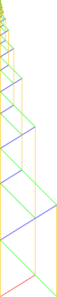
(c) Infinite run.

Figure 13: Meta-signals, rules and an infinite run of the machine $\mathfrak{M}_{gcd}^{\varphi}$.

With Lem. 8, we finally obtain:

Proposition 2.

There exists $3$-speed signal machines defined with an irrational ratio between either two speeds or two of its initial positions, that produce accumulations.

4.2 Case of rational-like machines

We show now that the existence of incommensurate values is a necessary condition for accumulating with some $3$-speed machine. This proof is done in two steps. First, we bring back the study of any rational-like $3$-speed machine to the study of a rational $3$-speed support machine (having speeds $-1$, $0$ and a third rational speed $\nu$). Second, we show that the diagrams of a rational $3$-speed support machine are included on some regular structures —called meshes— that cannot contain any accumulation.

4.2.1 Normalization of speeds

In the same way that we did for $2$-speed machines, we can reduce the problem of accumulating with $3$-speed machines to machines having speeds $-1$, $0$ and $\nu$ where $\nu$ is a real positive number.

Indeed, let $\mathfrak{M}^{a,b,c}$ be a signal machine having only three distinct speeds $a,b$ and $c$ with $a<b<c$. We define a machine $\mathfrak{M}^{-1,0,\nu}$, equivalent to $\mathfrak{M}^{a,b,c}$. Consider the function $h:\mathbb{R}\to\mathbb{R}$ defined in Subsect. 2.3, with $c=-1$ and $d=0$: $h(x)=\frac{x}{b-a}-\frac{b}{b-a}\enspace$. We have then $f(a)=-1$, $f(b)=0$ and $f(c)=\frac{c-b}{b-a}>0$. We call $\nu=f(c)$. By Lem. 1, since $h$ is an affine function of strictly positive ratio, diagrams of $\mathfrak{M}^{a,b,c}$ and $\mathfrak{M}^{-1,0,\nu}$ will be equivalent. In particular, if $\mathfrak{M}^{a,b,c}$ produces a space-time diagram including an accumulation, $\mathfrak{M}^{-1,0,\nu}$ will also produce a corresponding diagram including an accumulation.

In this section, we want to prove that no rational-like signal machine produces accumulation when started on rational-like initial configuration. As done for $2$ speeds, for any rational-like machine $\mathfrak{M}^{a,b,c}$, we will only consider by now the support signal machine $\widehat{\mathfrak{M}^{-1,0,\nu}}$ of the machine $\mathfrak{M}^{-1,0,\nu}$, equivalent to $\mathfrak{M}^{a,b,c}$, where $\nu=\frac{c-b}{b-a}$. The support machine $\widehat{\mathfrak{M}^{-1,0,\nu}}$ contains exactly $3$ meta-signals: one for each speed amoung $-1,0$ and $\nu$. Each collision rules of $\widehat{\mathfrak{M}^{-1,0,\nu}}$ outputs the maximal possible number of meta-signals, that is the $3$ meta-signals of the machine.

Note that if $\mathfrak{M}^{a,b,c}$ is rational-like, then $\mathfrak{M}^{-1,0,\nu}$ is a rational machine: if all ratios between $a$, $b$ and $c$ are rational, then $\nu$ will also be rational. Indeed, for any real non zero numbers $x,y$, the following holds: $\frac{x}{y}\in\mathbb{Q}\Longleftrightarrow\frac{x-y}{y}\in\mathbb{Q}\enspace.$ Since $\nu=\frac{c-b}{b-a}=\frac{c}{b-a}-\frac{b}{b-a}$, we deduce that $\frac{a}{b},\frac{a}{c}\in\mathbb{Q}\Rightarrow\nu\in\mathbb{Q}\enspace.$

So we will express $\nu$ in the form of a fraction $\nu=\frac{p}{q}$ where $p$ and $q$ are positive coprimes integer, so that the fraction is irreducible (and positive since $\nu$ is). To simplify the notation, we will note $\mathfrak{M}_{3}^{\nu}$ or $\mathfrak{M}_{3}^{p/q}$ to designate $\widehat{\mathfrak{M}^{-1,0,\nu}}$, the support machine having the $3$ rational speeds $-1,0$ and $\nu=\frac{p}{q}$.

4.2.2 Meshes and diagrams

We construct a family of diagrams such that every diagram generated by the support machine $\mathfrak{M}_{3}^{\nu}$ is included in one diagram of the family. Since no diagram in the family contains any ccumulation, the machine $\mathfrak{M}_{3}^{\nu}$ cannot produce an accumulation. This is done in two steps. In a first time, we show that diagrams obtained from a special form of initial configurations eventually become periodic: we call such a diagram a mesh. In a second time, we prove that any rational initial configuration $c_{0}$ of $\mathfrak{M}_{3}^{\nu}$ can be extended into one of the configurations that produce meshes and so there exists a mesh which includes the support diagram of the diagram started from $c_{0}$.

Notions of strips and meshes

We first introduce strips, which are used as the basic components of meshes. Recall that in this section, the speed $\nu$ is given by the rational number $p/q$, where $p,q\in\mathbb{N}$ are coprimes.

Definition 13 (Strip).

Let be $x_{0},w\in\mathbb{R}^{+}$. We call $(p,q,x_{0},w)$–$\mathcal{S}trip$ the diagram generated by $\mathfrak{M}_{3}^{\nu}$ from the initial configuration:

$$\left\{\ [\overleftarrow{\textsf{\sf{L}}},\overrightarrow{\textsf{\sf{R}}}]@{x_{0}},\ \textsf{\sf{S}}@{x_{0}+\frac{i}{p+q}\cdot w},\ [\overleftarrow{\textsf{\sf{L}}},\overrightarrow{\textsf{\sf{R}}}]@{x_{0}+w}\ \middle|\ 0\leq i\leq p+q\right\}\enspace.$$

Figure 14(b) displays a $(\frac{2}{3},5,0,1)$–$\mathcal{S}trip$ (the diagram has been croped on both sides, signals leaving on both sides are supposed to propagate indefinitely).

The parameter $x_{0}$ is the position of the begining of the strip i.e. the position of the left-most stationary signal, and $w$ is the total width of the strip (so the position of the right-most stationary is $x_{0}+w$). Parameters $p$ and $q$ (remember that we have the rational positive speed $\nu=p/q$) provides $p+q$, which the number of subdivisions of same length of the interval $[x_{0};x_{0}+w]$. This is the number of such subdivisions that would have been created during the evolution of the machine without placing all the initial stationary signals between the two extremal stationary signals, as illustrated by Fig. 14(a). Intuitively, it corresponds to the minimal number of divisions of the strip in equal parts so that all collisions between two signals $\overrightarrow{\textsf{\sf{R}}}$ and $\overleftarrow{\textsf{\sf{L}}}$ occurs exactly at the position of a subdivision So by placing a stationary signal S at each such position in the initial configuration every collision between $\overrightarrow{\textsf{\sf{R}}}$ and $\overleftarrow{\textsf{\sf{L}}}$ also involves S and is a triple collision.

So there are $p+q-1$ stationary signals between the left-most and the right-most stationary signals, and their position are $x_{0}+\frac{i}{p+q}\cdot w$ for $1\leq i\leq p+q-1$. Including the walls, a stationary signal S is set at each position $x_{0}+\frac{i}{p+q}$ for $0\leq i\leq p+q$. Figure 15(a) gives the geometrical meanings of a strip parameters.

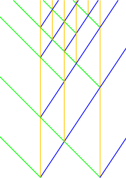
(a) An uncomplete strip.

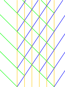
(b) A $(2,3,0,1)$–$\mathcal{S}trip$.

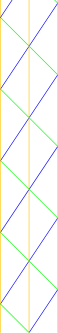
(c) Zig-zag on one and two subdivisions.

Figure 14: Basics structures for diagrams with $3$ speeds.

(a) Parameters of a $(p,q,x_{0},w)$–$\mathcal{S}trip$.

(b) Parameters of a $(p,q,x_{0},w,k)$–$\mathcal{M}esh$.

Figure 15: Parameters of strips and meshes.

We first prove two lemmata, stating that the structure of a strip is regular: in the central part of the strip, the diagram behaves with respect to a periodic pattern and space outside the central part contains only parallel signals that will never collide.

Lemma 9.

No collision can happen on the space outside the interval $[x_{0};x_{0}+w]$ in a $(p,q,x,w)$–$\mathcal{S}trip$.

Proof.

Any signal going crossing the left-most signal S, initially placed in $x_{0}$ is necessarily a signal $\overleftarrow{\textsf{\sf{L}}}$. By the form of the configuration $c_{0}$, there is no signal placed before the position $x_{0}$ and since signals going on the left side of the first stationary signal are all parallel, there is no possible collision on space before the position $x_{0}$. The same happens symetrically on the other side. ∎

We show next that for proper parameters, a strip is a regular structure, composed by a vertical grid with parallel signals leaving on both sides.

Lemma 10.

Any $(p,q,x_{0},w)$–$\mathcal{S}trip$ becomes periodic on the interval $[x_{0};x_{0}+w]$ after the time $t_{T}=\frac{q}{p+q}\cdot w$. After this time, the period is given by $T=\frac{w}{p}$.

This lemma means that for all $t\geq t_{T}$, for all $x\in[x_{0};x_{0}+w]$ we have: $c_{t+T}(x)=c_{t}(x)$. We cannot have a complete periodicity on the whole space because of signals leaving the strip on both sides. That is why we restrict the study of a strip evolution to the interval defined by the extremal stationary signals, that is the interval $[x_{0};x_{0}+w]$.

Proof.

Let us begin with a simple remark: for three signals S with same distance between the two first and the two last signals, times of back-and-forth of signals $\overleftarrow{\textsf{\sf{L}}}$ and $\overrightarrow{\textsf{\sf{R}}}$ starting both from the central S are the same, as illustrated by Fig. 14(c). Indeed, for two signals S spaced by a distance $l$ and a signal $\overrightarrow{\textsf{\sf{R}}}$ of speed $\nu$ starting from the first S, it will take a time $\nu l$ to $\overrightarrow{\textsf{\sf{R}}}$ for going the second S. After the collision, $\overrightarrow{\textsf{\sf{R}}}$ makes a bounce on S and is turned into a signal $\overleftarrow{\textsf{\sf{L}}}$ (of speed $-1$), which will need a time $1\cdot l$ to go back to the first S. The total time of the back-and-forth is $\nu l+l=(1+\nu)l$. The symetric back-and-forth (when starting with $\overleftarrow{\textsf{\sf{L}}}$ from the right S) requires the same amount of time $(1+\nu)l$. So for three signals S so that the middle S is at distance $l$ of the two other S, if one signal $\overleftarrow{\textsf{\sf{L}}}$ and one signal $\overrightarrow{\textsf{\sf{R}}}$ leave the central S at the same time, since the time of a back-and-forth is the same for both of them (because the distance to run is the same), they will collide with the central S exactly at the same time and the collision involved will be a triple collision. By the rules of a support machine, all possible signals will be output from this collision: $\overrightarrow{\textsf{\sf{R}}}$ and $\overleftarrow{\textsf{\sf{L}}}$ will leave at the same time and the previous computation will apply again. So from a triple collision, there will be a triple collisions after each duration $(1+\nu)l$. For the same reasons, this also holds for any number of signals S if two successive S are spaced by the same distance. In the case of a $(p,q,x_{0},w)$–$\mathcal{S}trip$, the speed is $\nu=\frac{p}{q}$, the distance between S signals is given by $\frac{w}{p+q}$ and so the time of a back-and-forth in a subdivision is $(1+\frac{p}{q})\cdot\frac{w}{p+q}=\frac{w}{q}$.

To claim that all collisions between a $\overrightarrow{\textsf{\sf{R}}}$ signal and a $\overleftarrow{\textsf{\sf{L}}}$ signal also involves a stationary signal S, it remains to show that the collision between the two non-stationary signals of the initial configuration happens exactly at the position of an initial S. Let us compute the coordinates of this “central” collision between the initial $\overrightarrow{\textsf{\sf{R}}}$ and $\overleftarrow{\textsf{\sf{L}}}$ signals, initially disposed at positions $x_{0}$ and $x_{0}+w$. This coordinates $(x_{C},t_{C})$ satisfy $\nu\cdot t_{C}+x_{0}=-t_{C}+x_{0}+w$ et $x_{C}=\nu\cdot t_{C}+x_{0}$, that is $x_{C}=\frac{\nu}{\nu+1}w+x_{0}$ and $t_{C}=\frac{w}{\nu+1}$. Since $\nu=\frac{p}{q}$, we get $x_{C}=\frac{p}{p+q}w+x_{0}$ and $t_{C}=\frac{q}{p+q}w$. So the position $x_{C}$ is $\frac{p}{p+q}w+x_{0}$ and can indeed be put in the form $x_{0}+\frac{i}{p+q}w$ where $0\leq i\leq n$, which corresponds to the position of an initial signal S.

With the remark made at the beginning of the proof, we can conclude that, from the time $t_{C}$, all collisions (except the ones happening on the two extremal walls) are triple collisions. Thus the diagram become periodic between the two walls (i.e. between positions $x_{0}$ and $x_{0}+w$) after the time $t_{T}=t_{C}$, and the duration of a period is given by the time of a back-and-forth i.e. $T=\frac{w}{q}$. ∎

Regarding the “external parts” of the strip, some signals are generated with a regular spacing and propagate indefinitely. On the left part, signals $\overleftarrow{\textsf{\sf{L}}}$ (moving on the left) are all spaced by a distance $d=(1+\frac{p}{q})\times\frac{w}{p+q}$, which is the distance covered by a signal $\overleftarrow{\textsf{\sf{L}}}$ during the time of a back-and-forth on a subdivision. On the right part, signals $\overrightarrow{\textsf{\sf{R}}}$ are all spaced by a horizontal distance $d=\frac{(1+\frac{p}{q})\cdot w\cdot p}{q(p+q)}$.

In fact, the number $p+q$ of subdivisions corresponds to $1/gcd\left(\frac{\nu}{\nu+1},1\right)$ (note that when $\nu$ is rationnal, this number is indeed an integer). This value is deduced from the study of the coordinates of the collision $C$. Any other multiple of $1/gcd\left(\frac{\nu}{\nu+1},1\right)$ for the number of subdivisions also allows to get a strip which becomes perdiodic after the time $t_{T}$ (the difference being that the subdivisions are more or less narrow in function of the multiple chosen).

From strips that we use as elementary structures, we can now define a more general and regular structure:

Definition 14 (Mesh).

Let be $k\in\mathbb{N}$ and $x_{0},w\in\mathbb{R}^{+}$. We call $(p,q,x_{0},w,k)$–$\mathcal{M}esh$ a diagram generated by $\mathfrak{M}_{3}^{\nu}$ from the initial configuration:

$$\left\{[\overleftarrow{\textsf{\sf{L}}},\textsf{\sf{S}},\overrightarrow{\textsf{\sf{R}}}]@{x_{0}+l\cdot w},\ \textsf{\sf{S}}@{x_{0}+\left(\frac{i}{p+q}+j\right)\cdot w}\ \middle|\ 0\leq l\leq k,\ 0<i<p+q\text{ and }0\leq j<k\right\}\enspace.$$

A $(p,q,x_{0},w,k)$–$\mathcal{M}esh$ corresponds to $k$ copies of a $(p,q,x_{0},w)$–$\mathcal{S}trip$ juxtaposed side by side so that the walls of two glued copies are superposed. Since all copies have the same parameters $w$ (the width) and $p+q$ (the number of equal subdivisions of $w$, also the number of zig-zag substrips), their substrips have all the same width given by $\frac{w}{p+q}$.

Note that a $(p,q,x_{0},w)$–$\mathcal{S}trip$ is a $(p,q,x_{0},w,1)$–$\mathcal{M}esh$. A $(2,3,0,1,3)$–$\mathcal{M}esh$ is given in Fig. 16: it corresponds to three copies of the strip given in Fig. 14(b).

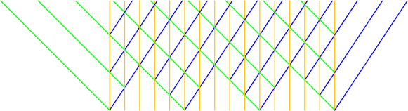
Figure 16: A $(2,3,0,1,3)$–$\mathcal{M}esh$.

The regularity of meshes can be deduced from the one of strips:

Lemma 11.

Any $(p,q,x_{0},w,k)$–$\mathcal{M}esh$ becomes periodic in the interval $[x_{0};x_{0}+k\cdot w]$, with a period $T=\frac{w}{p}$ and after the time $t_{T}=\frac{q}{p+q}\cdot w$.

Proof.

For all $j\in\llbracket 0;k-1\rrbracket$, the configuration

$$\left\{\ \textsf{\sf{S}}@{x_{0}+\left(\frac{i}{p+q}+j\right)\cdot w},\overleftarrow{\textsf{\sf{L}}}@{x_{0}+j\cdot w},\overrightarrow{\textsf{\sf{R}}}@{x_{0}+j\cdot w}\ \middle|\ 0\leq i\leq p+q\ \right\}$$

generates a $(p,q,x_{0}+jw,w)$–$\mathcal{S}trip$ (by definition of a strip). The initial configuration corresponding to the $(p,q,x_{0},w,k)$–$\mathcal{M}esh$ can be decomposed into such configurations (with a junction at each position $x=x_{0}+j\cdot w$). Since all these configurations correspond to strips having all the same parameters, back-and-forths in all subdivisions take the same duration. It follows from the proof of Lem. 10 that all collisions between signals $\overleftarrow{\textsf{\sf{L}}}$ and $\overrightarrow{\textsf{\sf{R}}}$ also involve stationary signals S, including the ones at the junction of two strips of the mesh. Since all strips are periodic with the same period from the same time $t_{C}$, the mesh is also periodic. Its period is the same that the strips and is given by Lem. 10: the $(p,q,x_{0},w,k)$–$\mathcal{M}esh$ is perdiodic in the interval $[x_{0};x_{0}+k\cdot w]$ with a period $T=\frac{w}{p}$ and from the time $t_{T}=\frac{q}{p+q}\cdot w$. ∎

One essential consequence of this lemma is the following corollary:

Corollary 3.

No accumulation can occur on a $(p,q,x_{0},w,k)$–$\mathcal{M}esh$.

Proof.

Because of Lem. 9, we just need to show that no accumulation occurs in the interval $[x_{0};x_{0}+k\cdot w]$. By Lem. 11, any mesh becomes periodic of period $T=\frac{w}{p}$, after a finite time $t_{T}$. There is only a finite number of collisions before the time $t_{T}$. For any time $t>t_{T}$, there can be only of finite number of collisions happening during the time interval $[t;t+T]$. Since a necessary condition for having an accumulation is the existence of a time interval during which an infinite number of collision occurs, no accumulation can appear in a mesh. ∎

Inclusion in a mesh

We show here that for any finite initial configuration $c_{0}$ having only rational ratio between distances, there is a configuration $c_{0}^{mesh}$ of a mesh $\mathcal{S}$ so that $c_{0}$ is included in $c_{0}^{mesh}$. It will follow directly that the whole diagram generated from $c_{0}$ is entirely included in $\mathcal{S}$. Figure 17 illustrates this idea, by providing an example of an arbitrary diagram and a mesh that includes the whole arbitrary diagram (extremal initial positions of the diagram of Fig. 17(a) match with those of Fig. 17(b)).

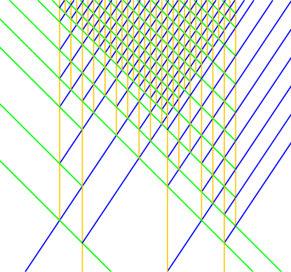
(a) Diagram $\mathbb{D}$ from an arbitrary initial configuration.

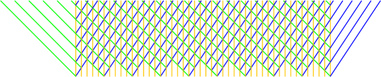
(b) The corresponding mesh $S$.

Figure 17: A diagram of $\mathfrak{M}_{3}^{\nu}$ and a mesh which includes it.

Lemma 12.

For every space-time diagram $\mathbb{D}$ generated by $\mathfrak{M}_{3}^{\nu}$ from a finite initial configuration having only rational ratio between distances, there exist $k\in\mathbb{N}$ and $x_{0},w\in\mathbb{R}$ so that $\mathbb{D}$ is included in a $(p,q,x_{0},w,k)$–$\mathcal{M}esh$.

Proof.

Let $c_{0}$ be a finite rational-like initial configuration i.e. $c_{0}=\{\sigma_{i}@x_{i}\ |\ x_{i}\in\mathbb{R}\}_{1\leq i\leq m}$ where $x_{1}\leq x_{2}\leq\ldots\leq x_{m}$ and so that for all $i,j,l\in\llbracket 0;m\rrbracket$ the value $\frac{x_{i}-x_{j}}{x_{j}-x_{l}}$ $(x_{j}\neq x_{l})$ is rational. Let $\mathbb{D}$ be a diagram generated by $\mathfrak{M}_{3}^{\nu}$ from $c_{0}$. Let us show that $\mathbb{D}$ is included in $\mathcal{S}$, the $(p,q,x_{0},w,k)$–$\mathcal{M}esh$ with parameters:

• $w=gcd(x_{1}-x_{0},x_{2}-x_{1},\ldots,x_{m}-x_{m-1})$,

• $k=\frac{x_{m}-x_{0}}{w}$.

These parameters are indeed valid parameters for a mesh: $w\in\mathbb{R}^{+}$ is well-defined because all ratios between distances in $c_{0}$ are rational (and is positive); and $k\in\mathbb{N}$ by definition of $w$. Note that $\mathcal{S}$ starts from the configuration $c_{0}^{\mathcal{S}}$ defined by:

$\left\{[\overleftarrow{\textsf{\sf{L}}},\textsf{\sf{S}},\overrightarrow{\textsf{\sf{R}}}]@{x_{0}+l\cdot w},\ \textsf{\sf{S}}@{x_{0}+\left(\frac{i}{p+q}+j\right)\cdot w}\ \middle|\ 0\leq l\leq k,\ 0<i<p+q,\ 0\leq j<k\right\}.$

It is enough to show that $c_{0}$ is included in $c_{0}^{\mathcal{S}}$ i.e. any signal $\sigma_{i}$ of $c_{0}$ at position $x_{i}$ is also present in $c_{0}^{\mathcal{S}}$ at the same position $x_{i}$. To prove this fact, we show that the position $x_{i}$ can be written $x_{i}=x_{0}+l\cdot w$, where $0\leq l\leq k$. Since there are always the three signals ($\overleftarrow{\textsf{\sf{L}}}$, S, $\overrightarrow{\textsf{\sf{R}}}$) at each of these positions, we don’t have to distinguish some subcases, according to $\sigma$ is either a signal S, $\overleftarrow{\textsf{\sf{L}}}$ or $\overrightarrow{\textsf{\sf{R}}}$.

The position $x_{i}$ can be written $x_{i}=x_{0}+l\cdot w$. Indeed, the value $w$ divides $x_{i}-x_{0}$ because $w=gcd(x_{1}-x_{0},x_{2}-x_{1},\ldots,x_{m}-x_{m-1})$, and it follows that there exists $l\in\mathbb{N}$ such that $x_{i}-x_{0}=l\cdot w$, that is: $x_{i}=x_{0}+l\cdot w$. Now let us show that $l$ satisfies the inequality of the definition of $c_{0}^{mesh}$ i.e. that we have $0\leq l\leq k$. For $i\in\llbracket 0;m\rrbracket$, we have:

$$\begin{array}[]{c r@{\ \leq\ } c r@{\ \leq\ } c r}0&&x_{i}-x_{0}&&x_{m}-x_{0}\\ 0&&l\cdot w&&x_{m}-x_{0}\\ 0&&l&&\frac{x_{m}-x_{0}}{w}&\text{ since $w>0$,}\\ 0&&l&&k&\text{ by definition of $k$.}\\ \end{array}$$

So any signal $\sigma$ at position $x_{i}$ in $c_{0}$ is also an initial signal in $c_{0}^{\mathcal{S}}$. Since $\mathfrak{M}_{3}^{\nu}$ is a support machine, it follows directly that $\mathbb{D}$ is included in the mesh $\mathcal{S}$. ∎

We finally obtain:

Theorem 1.

No $3$-speed rational-like signal machine can produce accumulation when started from a rational-like initial configuration.

Proof.

As mentionned in the paragraph on normalizations, every $3$-speed rational-like signal machine $\mathfrak{M}$ can be reduced to a $3$-speed machine having only rational speeds ($-1$, $0$ and $\nu$) and whom support machine is $\mathfrak{M}_{3}^{\nu}$. It holds by Coro. 1 that if $\mathfrak{M}_{3}^{\nu}$ started from a configuration doesn’t generate accumulations, then neither does $\mathfrak{M}$ (started from the same configuration). By Lemma 12, every diagram generated by $\mathfrak{M}_{3}^{\nu}$ started from a rational-like configuration is included in a mesh of $\mathfrak{M}_{3}^{\nu}$, and since a mesh doesn’t contain accumulation by Coro. 3, it follows that no accumulation can appear in any diagram of $\mathfrak{M}_{3}^{\nu}$, and so, also in any diagram of $\mathfrak{M}$ started from a rational-like configuration. ∎

5 Conclusion

We have shown that $2$-speed signal machines can’t have accumulations and that $4$-speed can freely create accumulations. Three-speed signal machines can only accumulate if there is an irrational ratio between speeds or between distances in the initial configuration.

The computing power of $2$-speed signal machines is very limited since the length of a computation is at most quadratic in the number of signals in the initial configuration. The last constructions in [Durand-Lose, 2011], provides a Turing-universal signal machine with four speeds. The case of $3$ speeds has been studied in [Durand-Lose, 2013]: the same dichotomy arises. In the rational-like case, the dynamics is cyclic with bounded transient time and period; otherwise, any Turing machine could be simulated. We conjecture that there is a similar dichotomy for hypercomputation.

References

- [Blum et al., 1989] Blum, L., Shub, M., and Smale, S. (1989). On a theory of computation and complexity over the real numbers: NP-completeness, recursive functions and universal machines. Bulletin of the American Mathematical Society, 21(1):1–46.
- [Bournez, 1997] Bournez, O. (1997). Some bounds on the computational power of piecewise constant derivative systems. In 24th International Colloquium on Automata, Languages and Programming (ICALP ’97), number 1256 in LNCS, pages 143–153.
- [Cook, 2004] Cook, M. (2004). Universality in elementary cellular automata. Complex Systems, 15(1):1–40.
- [Duchier et al., 2010] Duchier, D., Durand-Lose, J., and Senot, M. (2010). Fractal parallelism: Solving SAT in bounded space and time. In Cheong, O., Chwa, K.-Y., and Park, K., editors, 21st International Symposium on Algorithms and Computation (ISAAC ’10), number 6506 in LNCS, pages 279–290. Springer.
- [Duchier et al., 2012] Duchier, D., Durand-Lose, J., and Senot, M. (2012). Computing in the fractal cloud: modular generic solvers for SAT and Q-SAT variants. In Agrawal, M., Cooper, S. B., and Li, A., editors, 9th International Conference on Theory and Applications of Models of Computation (TAMC ’12), number 7287 in LNCS, pages 435–447. Springer.
- [Durand-Lose, 2008a] Durand-Lose, J. (2008a). Abstract geometrical computation with accumulations: Beyond the Blum, Shub and Smale model. In Beckmann, A., Dimitracopoulos, C., and Löwe, B., editors, Logic and Theory of Algorithms, 4th International Conference on Computability in Europe (CiE ’08) (abstracts and extended abstracts of unpublished papers), pages 107–116. University of Athens.
- [Durand-Lose, 2008b] Durand-Lose, J. (2008b). The signal point of view: From cellular automata to signal machines. In Durand, B., editor, Journées Automates cellulaires 2008 (JAC ’08), pages 238–249.
- [Durand-Lose, 2009a] Durand-Lose, J. (2009a). Abstract geometrical computation 3: Black holes for classical and analog computing. Nat. Comput., 8(3):455–572.
- [Durand-Lose, 2009b] Durand-Lose, J. (2009b). Abstract geometrical computation and computable analysis. In Costa, J. and Dershowitz, N., editors, 8th International Conference on Unconventional Computation 2009 (UC ’09), number 5715 in LNCS, pages 158–167. Springer.
- [Durand-Lose, 2011] Durand-Lose, J. (2011). Abstract geometrical computation 4: small Turing universal signal machines. Theoret. Comp. Sci., 412:57–67.
- [Durand-Lose, 2012] Durand-Lose, J. (2012). Abstract geometrical computation 7: Geometrical accumulations and computably enumerable real numbers. Nat. Comput., to appear. Special issue on Unconv. Comp. ’11.
- [Durand-Lose, 2013] Durand-Lose, J. (2013). Irrationality is needed to compute with signal machines with only three speeds. In Bonizzoni, P., Brattka, V., and Löwe, B., editors, The Nature of Computation, 9th International Conference on Computability in Europe (CiE ’13), LNCS. Springer. To appear.
- [Hardy and Wright, 1960] Hardy, G. H. and Wright, E. M. (1960). An Introduction to the Theory of Numbers (4th edition). Oxford University Press.
- [Huckenbeck, 1989] Huckenbeck, U. (1989). Euclidian geometry in terms of automata theory. Theoret. Comp. Sci., 68(1):71–87.
- [Jacopini and Sontacchi, 1990] Jacopini, G. and Sontacchi, G. (1990). Reversible parallel computation: an evolving space-model. Theoret. Comp. Sci., 73(1):1–46.
- [Margenstern, 2000] Margenstern, M. (2000). Frontier between decidability and undecidability: a survey. Theor. Comput. Sci., 231(2):217–251.
- [Mazoyer, 1996] Mazoyer, J. (1996). Computations on one-dimensional cellular automata. Annals of Mathematics and Artificial Intelligence, 16:285–309.
- [Mazoyer and Terrier, 1999] Mazoyer, J. and Terrier, V. (1999). Signals in one-dimensional cellular automata. Theoret. Comp. Sci, 217(1):53–80.
- [Mycka et al., 2006] Mycka, J., Coelho, F., and Costa, J. F. (2006). The Euclid Abstract Machine: Trisection of the Angle and the Halting Problem. In Calude, C. S., Dinneen, M. J., Paun, G., Rozenberg, G., and Stepney, S., editors, 5th International Conference on Unconventional Computation (UC ’06), number 4135 in LNCS, pages 195–206. Springer.
- [Ollinger and Richard, 2011] Ollinger, N. and Richard, G. (2011). Four states are enough! Theoret. Comp. Sci., 412(1-2):22–32.
- [Rogozhin, 1996] Rogozhin, Y. (1996). Small universal turing machines. Theoret. Comp. Sci., 168(2):215–240.
- [Weihrauch, 2000] Weihrauch, K. (2000). Computable Analysis: an introduction. Springer Verlag.
- [Woods and Neary, 2007] Woods, D. and Neary, T. (2007). Four small universal turing machines. In Durand-Lose, J. and Margenstern, M., editors, 5th International Conference on Machines, Computations, and Universality (MCU ’07), number 4664 in LNCS, pages 242–254. Springer.