Associating long-term $\gamma$-ray variability
with the superorbital period of LS I $+$61^∘303

Abstract

Gamma-ray binaries are stellar systems for which the spectral energy distribution (discounting the thermal stellar emission) peaks at high energies. Detected from radio to TeV gamma rays, the $\gamma$-ray binary LS I $+$61^∘303 is highly variable across all frequencies. One aspect of this system’s variability is the modulation of its emission with the timescale set by the $\sim 26.4960$-day orbital period. Here we show that, during the time of our observations, the $\gamma$-ray emission of LS I $+$61^∘303 also presents a sinusoidal variability consistent with the previously-known superorbital period of 1667 days. This modulation is more prominently seen at orbital phases around apastron, whereas it does not introduce a visible change close to periastron. It is also found in the appearance and disappearance of variability at the orbital period in the power spectrum of the data. This behavior could be explained by a quasi-cyclical evolution of the equatorial outflow of the Be companion star, whose features influence the conditions for generating gamma rays. These findings open the possibility to use $\gamma$-ray observations to study the outflows of massive stars in eccentric binary systems.

1 Introduction

LS I $+$61^∘303 is one of the few X-ray binaries that have been detected from radio to TeV gamma rays (see Albert et al. 2006 and references therein). It is perhaps the most intriguing one due to the high variability and richness of its phenomenology at all frequencies. LS I $+$61^∘303  consists of a Be star of approximately 10 solar masses, and a compact object. Be stars are rapidly rotating B-type stars showing hydrogen Balmer lines in emission in the stellar spectrum, and which lose mass to an equatorial circumstellar disc. The nature of the compact object in LS I $+$61^∘303 has been much debated over the past few years: Pulsar wind interaction (see e.g., Maraschi & Treves, 1981; Dubus, 2006; Zamanov et al., 2001; Torres et al., 2012) and microquasar jets (see Bosch-Ramon & Khangulyan, 2009 for a review) have been proposed as the origin of the non-thermal emission. The recent detection of two short ($<0.1$ s), highly-luminous ($>10^{37}$ erg s^-1), thermal flares Papitto et al. (2012) have given support to the hypothesis that the compact object in LS I $+$61^∘303 is a neutron star, for only highly-magnetized neutron stars have been found to behave in this way.

The flux of LS I $+$61^∘303 is seen to be modulated by the orbital period of 26.4960 days Gregory (2002) at most wavelengths, including at high energies Torres et al. (2010); Zhang et al. (2010); Abdo et al. (2009); Albert et al. (2008). Orbital modulation of the GeV flux can be understood as a consequence of changing conditions for generation and absorption of gamma rays, which are mostly determined by the orbital geometry; e.g., the viewing angle to the observer and the position of the compact object with respect to the stellar companion. Unless other physical conditions change, we do not expect long-term variability of the emission level at a fixed orbital configuration. In order to investigate LS I $+$61^∘303’s variability, we analyzed Fermi-Large Area Telescope (LAT) data from the beginning of scientific operations on 2008 August 4 until 2013 March 24. We report on the results in this Letter.

2 Data Analysis

We used the LAT Science Tools package (v9r30), which is available from the Fermi Science Support Center, as is the LAT data, together with the P7v6 version of the instrument response functions. Only events passing the Pass 7 “Source” class cuts are used in the analysis. All gamma rays with energies $>100$ MeV within a circular region of interest (ROI) of 10^∘ radius centered on LS I $+$61^∘303 were extracted. To reduce the contamination from the Earth’s upper atmosphere time intervals when the Earth limb was in the field of view were excluded, specifically when the rocking angle of the LAT was greater than $52^{\circ}$ or when parts of the ROI were observed at zenith angles $>100^{\circ}$. The $\gamma$-ray flux of LS I $+$61^∘303  plotted in the light curves of this work are calculated by performing the binned or the unbinned maximum likelihood method, depending on the statistics, by means of the Science Tool gtlike. The spectral-spatial model constructed to perform the likelihood analysis includes all the sources of the second Fermi-LAT point-source catalog Nolan et al. (2012) (hereafter 2FGL) within 15^∘ of LS I $+$61^∘303. The spectral parameters were fixed to the catalog values, except for the sources within 3^∘ of LS I $+$61^∘303. For these latter sources, the flux normalization was left free. LS I $+$61^∘303 was modeled with an exponentially cut off power-law spectral shape. All its spectral parameters were allowed to vary (see Hadasch et al., 2012 for further details). The models adopted for the Galactic diffuse emission (gal_2yearp7v6_v0.fits) and isotropic backgrounds (iso_p7v6source.txt) were those recommended by the LAT team.

Systematic errors mainly originate in the uncertainties in the effective area of the LAT, as well as in the Galactic diffuse emission model. The current estimate of the uncertainties of the effective area is 10% at 100 MeV, decreasing to 5% at 560 MeV and increasing to 10% at 10 GeV and above. We assume linear extrapolations, in log space, between the quoted energies. The systematic effect is estimated by repeating the likelihood analysis using modified instrument response functions that bracket the “P7SOURCE_V6” effective areas. Specifically, they are a set of Instrument Response Functions in which the effective area has been modified considering its uncertainty as a function of energy in order to maximally affect a specific spectral parameter. In order to conservatively take into account the effect due to the uncertainties of the Galactic diffuse emission model, the likelihood fits are repeated changing the normalization of the Galactic diffuse model artificially by $\pm 6\%$. We have found flux systematic errors (for energies above 100 MeV) on the order of 9%, similar to the ones reported in Hadasch et al., 2012.

3 Results

Fig. 1 shows the orbitally-folded light curve of LS I $+$61^∘303 from 2008 August 4 to 2013 March 24. It shows a trend for the maximum of the $\gamma$-ray emission to appear near periastron (phases around 0.3), as in Hadasch et al., 2012, and significant $\gamma$-ray flux variability at fixed orbital phases.

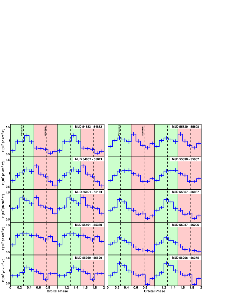
Figure 1: Gamma-ray flux from LS I $+$61^∘303 folded on the orbital period. The data are repeated over two cycles for clarity. Photons with energies above 100 MeV, as measured by Fermi-LAT are considered. The measurements cover the period from 2008 August 4 to 2013 March 24, from the top left panel to the bottom right. Each panel spans an equal interval of 169.2 days. The position of periastron and apastron are marked with dashed vertical lines (the ephemeris of Aragona et al., 2009 is used). The two background colors correspond to the periastron (orbital phases 0.0–0.5) and apastron (orbital phases 0.5-1.0) regions of the orbit.

We explore the possibility that the observed long term $\gamma$-ray variability could be related to the superorbital period of 1667$\pm$8 days as reported in radio and optical frequencies Gregory (2002). A variability signature with this period was also found along several years of X-ray observations Li et al. (2012); Chernyakova et al. (2012). Fig. 2 shows the long-term evolution of the average $\gamma$-ray flux; we use the superorbital period of Gregory (2002) to translate time to superorbital phase. The probability that this evolution is a random result out of a uniform distribution is $<1.1\times 10^{-12}$ ($\chi^{2}$, $ndf$ = 75.8, 9).

To check for a possible long-term modulation of the $\gamma$-ray flux at any orbital configuration, we have separated the data in orbital bins, and plotted the fluxes against the superorbital phase, as shown in Fig. 3. The black line in each of the panels of Fig. 3 represents a sinusoidal function fit to the data points. The period of this function has been kept (in all panels) at the value of the superorbital period found in radio (1667 days). Thus, the function we use to fit the data has three parameters: average flux level, amplitude, and phase. We have also fitted a constant line for comparison.

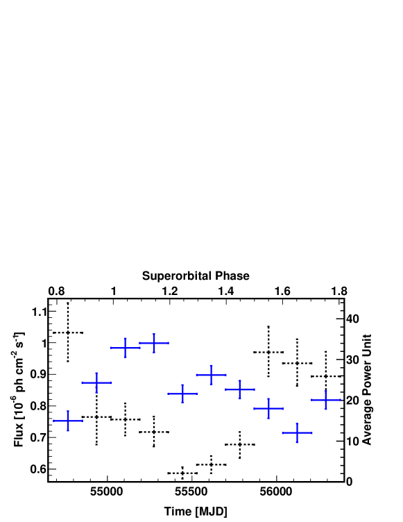
Figure 2: Long-term evolution of the average $\gamma$-ray flux (above 100 MeV) from LS I $+$61^∘303 (blue points, left y-axis scale). The superorbital phase is shown in the top axis. The right y-axis scale and the black dashed points show the long-term evolution of the power at the orbital period found in the Lomb-Scargle periodogram.

Table 1 shows the quality of the fitting results corresponding to Fig. 3. It has the following columns: the system’s orbital phase, the corresponding $\chi^{2}$ and dof as well as the probability that the data are described by either a constant or a sinusoidally varying flux, and finally the probability that the improvement found when fitting a sinusoid instead of a constant is produced by chance. To obtain the latter we consider the likelihood ratio test Mattox et al. (1996). The test is performed by computing the ratio $2\times\Delta log(Likelihood)$ for the two hypotheses (constant and sinusoidal) and assuming that for a chance coincidence the ratios are $\chi^{2}$-distributed according to the difference in the degrees of freedom between the two hypotheses. Thus, if the hypothesis of a constant is true, the likelihood ratio $R=-2\ln(L(constant)/L(sine))$ is approximately $\chi^{2}$-distributed with 2 degrees of freedom. The probability that one hypothesis is preferred over the other is defined as $P=\int_{0}^{R_{meas}}p(\chi^{2})d\chi^{2}$ where $p(\chi^{2})$ is the $\chi^{2}$ probability density function and $R_{meas}$ the measured value of $R$. The constant hypothesis will be rejected (and the sinusoidal will be accepted) if $P$ is greater than the confidence level, which is set to 95%. In Table 1, the last column states the probability that the fit improvement (of a sine over a constant) is happening by chance (thus, $1-P$).

Table 1: Quality of the fitting results corresponding to Fig. 3 (top panel) and sinusoidal fitting parameters for the flux near apastron (bottom panel).

Orbital	$\chi^{2}$, ndf	Constant Fit	$\chi^{2}$, ndf	Sine Fit	Prob. improvement
Phase	(constant)	Probability	(sine)	Probability	by chance
0.0–0.1	10, 9	$3.2\times 10^{-1}$	10, 7	$1.9\times 10^{-1}$	1.0
0.1–0.2	13, 9	$1.8\times 10^{-1}$	12, 7	$1.1\times 10^{-1}$	1.0
0.2–0.3	27, 9	$1.4\times 10^{-3}$	26, 7	$5.0\times 10^{-4}$	0.7
0.3–0.4	13, 9	$1.6\times 10^{-1}$	8, 7	$3.6\times 10^{-1}$	$7.0\times 10^{-2}$
0.4–0.5	15, 9	$9.9\times 10^{-2}$	6, 7	$5.4\times 10^{-1}$	$1.2\times 10^{-2}$
0.5–0.6	84, 9	$2.8\times 10^{-14}$	23, 7	$2.0\times 10^{-3}$	$<1.0\times 10^{-7}$
0.6–0.7	50, 9	$8.1\times 10^{-8}$	10, 7	$2.2\times 10^{-1}$	$<1.0\times 10^{-7}$
0.7–0.8	41, 9	$6.1\times 10^{-6}$	18, 7	$1.0\times 10^{-2}$	$1.4\times 10^{-5}$
0.8–0.9	100, 9	$2.4\times 10^{-17}$	8, 7	$3.0\times 10^{-1}$	$<1.0\times 10^{-7}$
0.9–1.0	50, 9	$9.1\times 10^{-8}$	10, 7	$2.2\times 10^{-1}$	$<1.0\times 10^{-7}$
Orbital	$F_{0}$	$A$	$\phi$
Phase	[$10^{-6}$ ph cm-2 s-1]	[$10^{-6}$ ph cm-2 s-1]
0.5–0.6	1.00$\pm$0.03	0.25$\pm$0.03	0.87$\pm$0.03
0.6–0.7	0.85$\pm$0.02	0.20$\pm$0.03	0.90$\pm$0.02
0.7–0.8	0.78$\pm$0.02	0.15$\pm$0.03	0.79$\pm$0.03
0.8–0.9	0.72$\pm$0.03	0.26$\pm$0.03	0.92$\pm$0.03
0.9–1.0	0.73$\pm$0.02	0.17$\pm$0.03	0.02$\pm$0.04

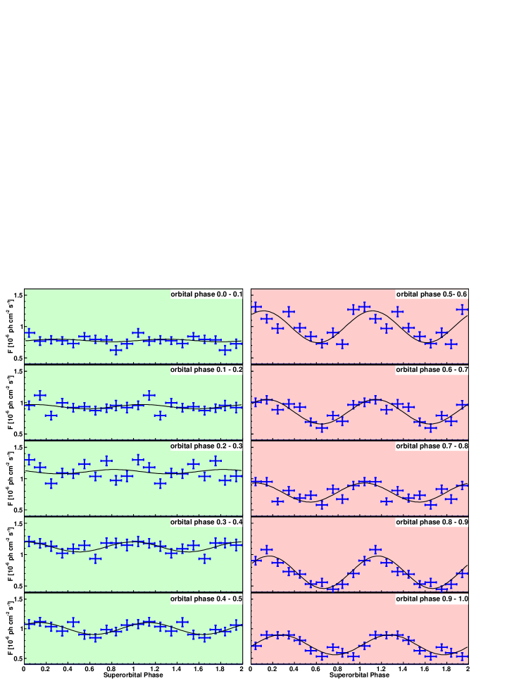
Figure 3: The evolution of the $\gamma$-ray flux (above 100 MeV) from LS I $+$61^∘303 at fixed orbital phases as a function of the superorbital phase. The data points are repeated over two superorbital periods for the sake of clarity. The left panels represent the region of the orbit near periastron (located at phase $\sim 0.3$, see Fig. 1) where the data are compatible with no superorbital variability beyond 3$\sigma$.). The right panels, instead, are regions close to apastron. The black line in each of the panels is a sinusoidal function fit to the data points, with a fixed period of 1667 days.

Table 1 also shows the sinusoidal fit parameters corresponding to the right-hand panels of Fig. 3. The functional form of the fit is $F_{0}+A\times\sin((t-T_{0})/T-\phi)\times 2\pi)$. Here, $T_{0}$ and $T$ are the zero time ($T_{0}$ = MJD 43366.275) and the period (always kept fixed at 1667 days in all panels) of the superorbit, respectively (both as in Gregory, 2002), $t$ is the time, $F_{0}$ is the average flux level, $A$ is the amplitude, and $\phi$ represents the phase shift in the superorbit. The choice of a sinusoidal function for fitting the data is not based on any a priori physical expectation; the superorbital variability could be periodic but have a different shape. However, any periodic function could be described by a series of sines. Thus, fitting with just one sinusoidal function as done above is motivated by the relatively low number of data points.

No strong variability is found at orbital phases 0.0–0.5, while it is clearly present in the range 0.5–1.0. Concurrently, data at the orbital phases 0.0 to 0.5 are not significantly better-represented by a sine than by a constant. However, this is not the case for the data at the orbital phases 0.5 to 1.0. The probability that the sinusoidal fit improvement occurs by chance is less than $1.0\times 10^{-7}$ at orbital phases 0.5–0.6, 0.6–0.7, 0.8–0.9, and 0.9–1.0; and $1.4\times 10^{-5}$ at orbital phases 0.7-0.8. Whereas the sinusoidal variation is always a better fit in this part of the orbit, the amplitude of the fit is maximal in orbital phases before and after the apastron.

In order to test for the appearance/disappearance of the orbital signature in gamma rays, we subdivided the data into the same time intervals of Fig. 1 and applied the Lomb-Scargle periodogram technique Lomb (1976); Scargle (1982) to each of them. To calculate the power spectrum the event selection was restricted to a ROI of 3^∘ radius centered on LS I $+$61^∘303. The selected events were used to create a light curve of weighted counts over exposure with equally spaced time bins of 2.4 hours width. The weight associated to each event corresponds to the probability that the $\gamma$-ray was emitted by LS I $+$61^∘303, rather than by nearby sources or has a diffuse origin The weights are calculated using the Science Tool gtsrcprob, adopting the best spectral-spatial models obtained by the binned likelihood fits described in the previous section. Before calculating the power spectrum, we also applied to the light curve the exposure weighting described in Corbet et al., 2007. Fig. 4 shows the power spectra calculated in each of the time intervals. The vertical line marks the orbital period (as in Gregory, 2002). The y-axis in the periodograms is given in average power units, which converts the original spectrum in units of (ph cm^-2 s^-1)² by normalizing it with the average of the power over all the frequencies $<P>$. In this way, the units are directly linked to the significance of the peak, which for a peak of power $\bar{P}$ is computed as ${\rm Prob}(P>\bar{P})=\exp{(-\bar{P}/<P>)}$ Scargle (1982). These average power values are plotted in Fig. 2. A significant peak is detected at the orbital period, but not in all time intervals. Note that in some of the panels of Fig. 4 there appears to be a shift of the 26.5-day peak, even though it is within the fundamental frequency ($1/T_{obs}$) of the orbital period. A claim that the period shift of these peaks is significant would then imply a severe oversampling of the Fourier resolution, which for the duration of this dataset is 3.84 days. The shifted peaks are not significant either in the single-trial (looking for an specific frequency) or in the all-trials probability analysis of these power spectra. Thus, we have now found that along the time covered by our observations, the power spectrum peak at the orbital period is significant only at superorbital phases $\sim 0.5-1.0$. At other superorbital phases, the peak is absent or has a significance less than 3$\sigma$.

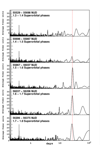
Figure 4: Periodogram of the $\gamma$-ray data for different time intervals. The dashed line marks the orbital period of LS I $+$61^∘303.

4 Discussion

Over the last two decades, systematic monitoring of many Be X-ray systems allowed the discovery of many cases of superorbital cycles (see, e.g., Alcock et al., 2001, Rajoelimanana et al., 2011). Thus, in order to connect the discovered $\gamma$-ray observational pattern to conditions that vary over the superorbit, a quasi-cyclical expansion and shrinking of the circumstellar disc of a Be star may offer an alternative (e.g., Negueruela et al., 2001). The sizes of the stellar discs of Be stars are hypothesized to correlate with the equivalent width (EW) of the H$\alpha$ emission line (e.g., Grundstrom et al., 2006). In the longest-running campaign observing LS I $+$61^∘303  the maximum of the H$\alpha$ EW has been found in a broad region around superorbital phase $0.2$ (see Zamanov et al., 1999; Zamanov & Martí, 2000 and references therein). Thus, the X-ray Li et al. (2012) as well as the $\gamma$-ray emission are enhanced at superorbital phases where maximal values of the H$\alpha$ EW have been measured. Concurrently, the power spectrum peak at the orbital period is less significant. This suggests that the disc may play a role in modulating both the gamma and the X-ray signals.

From the results in Fig. 3, one may conclude that in the periastron region, when the emission from the system is subject to essentially no superorbital variability, the conditions for the generation of gamma rays in the GeV range must not significantly change. We can thus assume that the compact object could be inside or severely affected by the Be disc matter when it is closer to the companion star (i.e., at orbital phases 0.0 to 0.5), for all superorbital phases. If this is the case, even when the EW of the H$\alpha$ line (and thus the radius within which the disc influences) changes by a factor of a few along the superorbital period , this does not necessarily imply a significant change in the $\gamma$-ray modulation above the sensitivity of Fermi-LAT when the compact object is near periastron. However, in a two-component model typically assumed for Be stellar winds (an equatorial wind generating the disc, and a polar outflow) the conditions in the apastron region (e.g., the pressure exerted by the wind, or the mass gravitationally captured by the compact object) could change by more than 3 orders of magnitude if one or the other component dominates (see, e.g., Gregory & Neish, 2002 and references therein). In such a case, it is reasonable to suppose that the GeV emission would be affected at an observable level.

We notice from Fig. 3 that between the orbital phase ranges 0.9–1.0 and 0.0–0.1 there is a significant change of the long-term behavior of the $\gamma$-ray emission. Closer to periastron the flux evolution flattens. We can then estimate the radius at which the matter in the disc of the Be star produces a stable influence with time by computing the system separation at orbital phase $\sim 0.1$. Using the ephemeris given by Aragona et al. (2009), we obtain a separation of $\sim 9R_{s}$, where $R_{s}$ is the stellar radius of the Be star. On the other hand, from the fact that the maximal amplitude of the superorbital variability is before and after the apastron of the system, the system separation at orbital phases 0.7 and 0.9 ($\sim 13R_{s}$) could also have a physical meaning. It is a qualitative upper limit to the influence of the matter in the equatorial outflow when maximally enhanced by the long-term change of the stellar mass-loss rate.

The ratio between what appears to be the maximal and the stable radii of influence of the disc matter is consistent with a possible increase of the EW of the H$\alpha$ line. Outer radii of discs in binaries are expected to be truncated by the gravitational influence of their compact companions; at the periastron distances in systems of high eccentricity, and by resonances between the orbital period and the disc gas rotational periods in the low-eccentricity systems Okazaki et al. (2001). LS I $+$61^∘303 is a system between these two cases. The effects of the Be star’s rotation, which have only recently started to be taken into account, may modify this conclusion, predicting disc sizes in excess of 10 $R_{s}$ Lee (2013). Assuming the relation between disc size and the EW of the H$\alpha$ by Grundstrom et al. (2006), and not taking into account rotation effects, typical values of the EW of LS I $+$61^∘303 would lead to an estimation of the disc radius of the order of the periastron distance Grundstrom et al. (2007). Simulations indicate that tidal pulls at periastron can lead to the development of large spiral waves in the disc that can extend far beyond the truncation radius and out to the vicinity of the companion (see e.g., Okazaki et al., 2001), promoting accretion Grundstrom et al. (2007). The $\gamma$-ray data apparently provide a window to infer the extent of these waves.

Depending on the period and dipolar magnetic field, a highly-magnetized neutron star can transition between states along the orbital evolution of LS I $+$61^∘303, changing its behavior from propeller (near periastron) to ejector (near apastron) along each orbit Zamanov et al. (2001); Torres et al. (2012); Papitto et al. (2012). These changes of state can be affected by the superorbital variability, since for a larger disc-influence radius, the system will remain in the same environment for a longer time Papitto et al. (2012). The orbital variability is consequently reduced, leading to the disappearance of the orbital peak in the power spectrum Torres et al. (2012). The data presented in this report will put the details of this model to the test while opening the $\gamma$-ray window for studying the discs of Be binaries.

References

- Abdo et al. (2009) Abdo, A. A., Ackermann, M., Ajello, M., et al. 2009, ApJ 701, L123
- Albert et al. (2006) Albert, J., Aliu, E., Anderhub, H., et al. 2006, Science 312, 1771
- Albert et al. (2008) Albert, J., Aliu, E., Anderhub, H., et al. 2008, ApJ 684, 1351
- Alcock et al. (2001) Alcock, C., Allsman, R. A., Alves, D. R., et al. 2001, MNRAS 321, 678
- Aragona et al. (2009) Aragona, C., McSwain, M. V., Grundstrom, E. D., Marsh, A. N., Roettenbacher, R. M., Hessler, K. M., Boyajian, T. S., & Ray, P. S. 2009, ApJ 698, 514
- Bosch-Ramon & Khangulyan (2009) Bosch-Ramon, V., & Khangulyan, D. 2009, Int. J. Mod. Phys. D 18, 347
- Chernyakova et al. (2012) Chernyakova, M., Neronov, A., Molkov, S., Malyshev, D., Lutovinov, A., Pooley, G. 2012, ApJ 747, L29
- Corbet et al. (2007) Corbet, R. H. D., Markwardt, C. B., & Tueller, J. 2007, ApJ 655, 458
- Dubus (2006) Dubus, G. 2006, A&A 456, 801
- Gregory (2002) Gregory, P. C. 2002, ApJ 575, 427 (2002).
- Gregory et al. (1989) Gregory, P. C., Xu, H.-J., Bachhouse, C. J., & Reid, A. 1989, ApJ 339, 1054
- Gregory & Neish (2002) Gregory, P. C., & Neish, C. 2002, ApJ 580, 1133
- Grundstrom et al. (2006) Grundstrom, E. D., & Gies, D. R. 2006, ApJ 651, L53
- Grundstrom et al. (2007) Grundstrom, E. D., Caballero-Nieves, S. M., Gies, D. R., et al. 2007, ApJ 656, 437
- Hadasch et al. (2012) Hadasch, D., Torres, D. F., Tanaka, T., et al. 2012, ApJ 749, 54
- Lee (2013) Lee, U. 2013, PASJ in press, arXiv:1304.6471
- Li et al. (2012) Li, J., Torres, D. F., Zhang, S., et al. 2012, ApJ 744, L13
- Lomb (1976) Lomb, N. R. 1976, Ap&SS 39, 447
- Maraschi & Treves (1981) Maraschi, L., & Treves, A. 1981, MNRAS 194, 1P
- Mc Swain et al. (2010) McSwain, M. V., Grundstrom, E. D., Gies, D. R., & Ray, P. S. 2010, ApJ 724, 379
- Mattox et al. (1996) Mattox, J. R., et al. 1986, ApJ 461, 396
- Negueruela et al. (2001) Negueruela, I. Okazaki, A. T., Fabregat, J., Coe, M. J., Munari, U., Tomov, T. 2001, A&A 369, 117
- Nolan et al. (2012) Nolan, P. L., et al. 2012, Astrophys. J. Suppl. 199, 31
- Okazaki et al. (2001) Okazaki, A. T., & Negueruela, I. 2001, A&A 377, 161
- Papitto et al. (2012) Papitto A., Torres D. F., & Rea N. 2012, ApJ 756, 188
- Rajoelimanana et al. (2011) Rajoelimanana, A. F., Charles, P. A., & Udalski, A. 2011, MNRAS 413, 1600
- Scargle (1982) Scargle, J. D. 1982, ApJ 263, 835
- Torres et al. (2010) Torres, D. F., Zhang, S., Li, J., et al. 2010, ApJ 719, L104
- Torres et al. (2012) Torres, D. F., Rea, N., Esposito, P., et al. 2012, ApJ 744, 106
- Zamanov et al. (1999) Zamanov, R. K., Martí, J., Paredes, J. M., et al. 1999, A&A 351, 543
- Zamanov & Martí (2000) Zamanov, R. K., & Martí, J. M. 2000, A&A 358, 55
- Zamanov et al. (2001) Zamanov, R. K., Martí, J. M., & Marziani, P. 2001, The Second National Conf. Astrophysics of Compact Objects, p. 50, arXiv:astro-ph/0110114
- Zamanov et al. (2007) Zamanov, R. K., Stoyanov, K. A., & Tomov, N. A. 2007, Information Bulletin on Variable stars 5776
- Zhang et al. (2010) Zhang, S., Torres, D. F., Li, J., et al. 2010, MNRAS 408, 642