Analytical transformed harmonic oscillator basis for
three-body nuclei of astrophysical interest: Application to ⁶He

Abstract

Recently, a square-integrable discrete basis, obtained performing a simple analytical local scale transformation to the harmonic oscillator basis, has been proposed and successfully applied to study the properties of two-body systems. Here, the method is generalized to study three-body systems. To test the goodness of the formalism and establish its applicability and limitations, the capture reaction rate for the nucleosynthesis of the Borromean nucleus ⁶He (${}^{4}\text{He}+n+n$) is addressed. Results are compared with previous publications and with calculations based on actual three-body continuum wave functions, which can be generated for this simple case. The obtained results encourage the application to other Borromean nuclei of astrophysical interest such as ⁹Be and ¹²C, for which actual three-body continuum calculations are very involved.

I Introduction

The study of three-body Borromean nuclei is known to be important for astrophysical questions such as stellar nucleosynthesis. Borromean nuclei are three-body systems whose binary subsystems are unbound Zhukov93 . One of the Borromean nuclei which has attracted more interest is ¹²C $(\alpha+\alpha+\alpha)$ due to the relevance of the triple-$\alpha$ reaction in the red giant phase of stars Hoyle . This process allows the formation of heavier elements in stars, where mainly $\alpha$ particles and nucleons are present, overcoming the $A=5$ and $A=8$ instability gaps Aprahamian05 . The production rate of such process has not yet been determined accurately for the entire temperature range relevant in astrophysics Nguyen1 . This is due to experimental problems to measure these processes as well as to discrepancies in the theoretical predictions about the structure of ¹²C. The formation of ¹²C has traditionally been studied as a sequential process Efros96 ; Sumiyoshi02 ; Bartlett06 . But, at low temperatures, the three $\alpha$ particles have no access to intermediate resonances and therefore they fuse directly Nguyen1 . The description of this process requires an accurate three-body model.

Other Borromean nuclei are also important for nucleosynthesis in different astrophysical scenarios. For instance, massive stars usually end up with the explosion of a supernova and the possible formation of a neutron star. These neutron-rich environments, with low density and high temperature (hot bubbles), are an ideal medium for nucleosynthesis by rapid neutron capture (or r-process) Meyer92 ; Meyer94 . Among these processes one finds the formation of ⁶He $(\alpha+n+n)$ or ⁹Be $(\alpha+\alpha+n)$ that could also overcome the $A=5,8$ gaps Bartlett06 . Therefore, as in the case of the triple-$alpha$ capture, understanding of these processes requires a very accurate description of the states of ⁶He and ⁹Be in a three-body model as well as the corresponding electromagnetic transition probabilities.

In particular, the ⁶He nucleus has a halo structure. The halo nuclei are weakly-bound exotic systems in which one or more particles have a large probability of being at distances far away from typical nuclear radii Hansen95 . A common characteristics of these systems is their small separation energy and hence their large breakup probability. This process can be understood as an excitation of the nucleus to unbound or scattering states that form a continuum of energies JALay10 . For that reason, the study of weakly bound three-body systems, such as ⁶He, demands a proper treatment of the three-body problem with a reasonable description of their continuum structure. In this work, a method, which includes these characteristics, is proposed and then applied to ⁶He as a benchmark calculation. It is worth noting that more fundamental few-body methods can be applied to ⁶He considered as a six-nucleon system, such as the Resonating Group Tang78 or the Lorentz Integral Transform Efros94 ; Bacca02 methods.

From the theoretical point of view, the treatment of unbound states of a quantum-mechanical system deals with the drawback that the corresponding wave functions are not square-normalizable and their energies are not discrete values. Solving this problem is a difficult task, especially as the number of charged particles increases, since one needs to know the asymptotic behavior of the unbound states. Nevertheless, there are various procedures to address this problem such as the R-matrix method Wigner47 ; IJThompson00 ; Desc06 , not without difficulties. Another approach to solve the continuum problem consists in using the so-called discretization methods. These methods replace the true continuum by a finite set of normalizable states, i.e., a discrete basis that can be truncated to a relatively small number of states and nevertheless provide a reasonable description of the system. Several discretization methods have been proposed Zhukov93 . For instance, one can solve the Schrödinger equation in a box RdDiego10 , being the energy level density governed by the size of the box. As this is larger, the energy level density increases but numerical problems begin to appear. Another method is the binning procedure, used traditionally in the Continuum-Discretized Coupled-Channels (CDCC) formalism Austern87 . In this method the continuum spectrum is truncated at a maximum energy and divided into a finite number of energy intervals or bins. For each bin, a normalizable state is constructed by superposition of the scattering states within that interval. This approach requires, first the calculation of the unbound states and then the matching with the correct asymptotic behavior. As mentioned above, the calculation of this asymptotic behavior for a three-body system with charged particles is by no means an easy task.

An alternative method to obtain a discrete representation of the continuum spectrum is the pseudostate (PS) method, which consists in diagonalizing the three-body Hamiltonian in a complete set of $\mathcal{L}^{2}$ wave functions (that is, square integrable). The eigenstates of the Hamiltonian are then taken as a discrete representation of the spectrum of the system. The advantage of this procedure is that it does not require going through the continuum wave functions and the knowledge of the asymptotic behavior is not needed. A variety of bases have been proposed for two-body HaziTaylor70 ; Matsumoto03 ; MRoGa04 ; AMoro09 and also for three-body calculations Matsumoto04 ; Rasoanaivo89 ; MRoGa05 .

In previous works, a PS method based on a local scale transformation (LST) of the harmonic oscillator (HO) basis has been proposed FPeBe01 . When the ground state of the system is known, a useful procedure to discretize the continuum consists in performing a numerical LST that transforms the actual ground-state wave function of the system into the HO ground state. Once the LST is obtained, the inverse transformation is applied to the HO basis, giving rise to the transformed harmonic oscillator (THO) basis. This method has been used to describe the two-body continuum in structure MRoGa04 and reactions AMoro01 ; AMoro06 studies, showing that the THO method together with the CDCC technique is useful to describe continuum effects in nuclear collisions. The method was also applied to ⁶He MRoGa05 ; MRoGa08 , showing that the numerical THO method is appropriate to describe three-body weakly bound systems with a relative small THO basis. In most recent works AMoro09 ; JALay10 an alternative prescription to define the LST was proposed, introducing an analytical transformation taken from Karataglidis et al. Karataglidis . This analytical transformation keeps the simplicity of the HO functions, but converts their Gaussian asymptotic behavior into an exponential one, more appropriate to describe bound systems. This analytical THO method has been applied to study two-body systems, providing a suitable representation of the bound and unbound spectrum to calculate structure and scattering observables within the CDCC method AMoro09 . The analytical THO presents several advantages over the numerical THO. (1) It is not needed to know previously the ground-state wave function of the system considered. (2) Due to the analytical form of the transformation, it can be easily implemented in a numerical code. (3) The parameters of the transformation govern the radial extension of the THO basis allowing the construction of an optimal basis for each observable of interest.

In this work, we extend the analytical THO method to study three-body systems. We start with the construction of the basis, then we diagonalize the three-body Hamiltonian, and we compute the transition probabilities needed for the calculation of the reaction rate. As a simple example of application, we check the formalism for the Borromean nucleus ⁶He. For this, a rich variety of data is available Aksough03 ; Egelhof03 ; Aumann98 ; Aumann99 ; Aguilera01 ; Aguilera00 ; Kakuee03 and can be used to benchmark theoretical models. Finally, the structure calculation allows us to determine the rate of the radiative capture reaction ${}^{4}\text{He}+n+n\rightarrow$ ${}^{6}\text{He}+\gamma$. It is known this reaction is not of great astrophysical interest but provides a robust test for our three-body model. In this case, with just one charged particle, one can generate easily the continuum wave functions and our model results can be confronted to actual continuum calculations. The study of this reaction will validate our formalism so as to make it reliable when applied to cases in which such comparisons with the true continuum cannot be easily done. This will be the case of ⁹Be, ¹²C, or ¹⁷Ne, that are subjects for future research.

The manuscript is structured as follows. In Sec. II the analytical THO method for three-body systems is completely worked out: basis, matrix elements, and calculation of transition probabilities. In Sec. III the expressions and concepts involved in the calculation of the radiative capture reactions of three particles into a bound nucleus are discussed. In Sec. IV the full formalism is applied to the case of ⁶He. Finally, in Sec. V, the main conclusions of this work are summarized.

II PS Method: Analytical THO for three-body systems

Jacobi coordinates $\{\boldsymbol{x},\boldsymbol{y}\}$, illustrated in Fig. 1, are used to describe three-body systems [six-dimensional problems]. The variable $\boldsymbol{x}$ is proportional to the relative coordinate between two of the particles and $\boldsymbol{y}$ is proportional to the coordinate from the center of mass of these two particles to the third one, both with a scaling factor depending on their masses MRoGa05 . Please, note that there are three different Jacobi systems. From the Jacobi coordinates, one can define the hyperspherical coordinates $\{\rho,\alpha,\widehat{x},\widehat{y}\}$, where $\rho=\sqrt{x^{2}+y^{2}}$ is the hyper-radius and $\tan\alpha=x/y$ defines the hyperangle.

The PS method consists in diagonalizing the Hamiltonian of the system of interest in a discrete basis of $\mathcal{L}^{2}$ functions. Using hyperspherical coordinates, and introducing $\Omega\equiv\{\alpha,\widehat{x},\widehat{y}\}$ for the angular dependence, the state wave functions of that basis can be expressed as

$$\psi_{i\beta j\mu}(\rho,\Omega)=R_{i\beta}(\rho)\mathcal{Y}_{\beta j\mu}(\Omega).$$ (1)

Here $\mathcal{Y}_{\beta j\mu}(\Omega)$ are states of good total angular momentum, expanded in hyperspherical harmonics (HH) Zhukov93 ; MRoGaTh $\Upsilon_{Klm_{l}}^{l_{x}l_{y}}(\Omega)$ as

$$\mathcal{Y}_{\beta j\mu}(\Omega) = \sum_{\nu\iota}\langle j_{ab}\nu I\iota|j\mu\rangle\kappa_{I}^{\iota}$$ (2)

$$\times \sum_{m_{l}\sigma}\langle lm_{l}S_{x}\sigma|j_{ab}\nu\rangle\Upsilon_{Klm_{l}}^{l_{x}l_{y}}(\Omega)\chi_{S_{x}}^{\sigma},$$

and $\beta\equiv\{K,l_{x},l_{y},l,S_{x},j_{ab}\}$ is a set of quantum numbers called channel. In this set, $K$ is the hypermomentum, $l_{x}$ and $l_{y}$ are the orbital angular momenta associated with the Jacobi coordinates $\boldsymbol{x}$ and $\boldsymbol{y}$, respectively, $l$ is the total orbital angular momentum ($\boldsymbol{l}=\boldsymbol{l_{x}}+\boldsymbol{l_{y}}$), $S_{x}$ is the spin of the particles related by the coordinate $\boldsymbol{x}$, and $j_{ab}$ results from the coupling $\boldsymbol{j_{ab}}=\boldsymbol{l}+\boldsymbol{S_{x}}$. If we denote by $I$ the spin of the third particle, which we assume to be fixed, the total angular momentum $j$ is $\boldsymbol{j}=\boldsymbol{j_{ab}}+\boldsymbol{I}$. With that notation, $\chi_{S_{x}}^{\sigma}$ is the spin wave function of the two particles related by the Jacobi coordinate $\boldsymbol{x}$, and $\kappa_{I}^{\iota}$ is the spin function of the third particle. The HH are eigenfunctions of the hypermomentum operator $\widehat{K}^{2}$, and can be expressed in terms of the spherical harmonics as

$$\Upsilon_{Klm_{l}}^{l_{x}l_{y}}(\Omega) = \sum_{m_{x}m_{y}}\langle l_{x}m_{x}l_{y}m_{y}|lm_{l}\rangle\Upsilon_{K}^{l_{x}l_{y}m_{x}m_{y}}(\Omega),$$ (3)

$$\Upsilon_{K}^{l_{x}l_{y}m_{x}m_{y}}(\Omega) = \varphi_{K}^{l_{x}l_{y}}(\alpha)Y_{l_{x}m_{x}}(\widehat{x})Y_{l_{y}m_{y}}(\widehat{y}),$$ (4)

$$\varphi_{K}^{l_{x}l_{y}}(\alpha) = N_{K}^{l_{x}l_{y}}(\sin\alpha)^{l_{x}}(\cos\alpha)^{l_{y}}$$ (5)

$$\times P_{n}^{l_{x}+\frac{1}{2},l_{y}+\frac{1}{2}}(\cos 2\alpha)$$

where $P_{n}^{a,b}$ is a Jacobi polynomial with order $n=(K-l_{x}-l_{y})/2$ and $N_{K}^{l_{x}l_{y}}$ is the normalization constant.

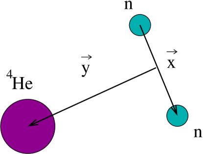
Figure 1: (Color online) The Jacobi $T$-coordinate system used to describe the ⁶He nucleus.

On the other hand, $R_{i\beta}(\rho)$ are the hyperradial wave functions, where the label $i$ denotes the hyperradial excitation. The form of these functions depends on the PS method used. Then, the states of the system are given by diagonalization of the three-body Hamiltonian in a finite basis up to $i_{\rm max}$ hyperradial excitations in each channel,

$$\Psi_{nj\mu}(\rho,\Omega)= \sum_{\beta}\sum_{i=0}^{i_{max}}C_{n}^{i\beta j}\psi_{i\beta j\mu}(\rho,\Omega)$$

$$= \sum_{\beta}\underbrace{\left(\sum_{i=0}^{i_{\rm max}}C_{n}^{i\beta j}R_{i\beta}(\rho)\right)}_{\mathcal{R}^{nj}_{\beta}(\rho)}\mathcal{Y}_{\beta j\mu}(\Omega),$$ (6)

being $C_{n}^{i\beta j}$ the diagonalization coefficients and $\mathcal{R}^{nj}_{\beta}(\rho)$ the hyperradial wave function corresponding to the channel $\beta$. The label $n$ enumerates the eigenstates.

II.1 Analytical THO method

As stated in the introduction, several PS bases have been proposed for three-body studies Matsumoto04 ; Rasoanaivo89 ; MRoGa05 ; FPeBe01 . Here, we use the THO method based on a LST of the HO functions, so the hyperradial wave functions are obtained as

$$R_{i\beta}^{\text{THO}}(\rho)=\sqrt{\frac{ds}{d\rho}}R_{iK}^{\text{HO}}[s(\rho)].$$ (7)

Note that, meanwhile the THO hyperradial wave functions depend, in general, on all the quantum numbers included in a channel $\beta$, the HO hyperradial wave functions only depend on one of them, the hypermomentum $K$. The transformation $s(\rho)$ is not unique, and in this work we adopt the analytical form of Karataglidis et al. Karataglidis ,

$$s(\rho)=\frac{1}{\sqrt{2}b}\left[\frac{1}{\left(\frac{1}{\rho}\right)^{\xi}+\left(\frac{1}{\gamma\sqrt{\rho}}\right)^{\xi}}\right]^{\frac{1}{\xi}},$$ (8)

depending on the parameters $\xi$, $\gamma$, and the oscillator length $b$. The HO hyperradial variable $s$ is dimensionless according to the transformation defined above [Eq. (8)]. In this way, we take the oscillator length $b$ as another parameter of the transformation.

The function $s(\rho)$ behaves asymptotically as $\frac{\gamma}{b}\sqrt{\frac{\rho}{2}}$ and hence the THO hyperradial wave functions obtained behave at large distances as $\exp{(-\gamma^{2}\rho/2b^{2})}$. Therefore, the ratio $\gamma/b$ governs the asymptotic behavior of the THO functions: as $\gamma/b$ increases, the hyperradial extension of the basis decreases and some of the eigenvalues obtained by diagonalizing the Hamiltonian explore higher energies JALay10 . That is, $\gamma/b$ determines the density of PSs as a function of the energy. Concerning the parameter $\xi$, the authors of Ref. Karataglidis found a very weak dependence of the results on this parameter. Because of that, we have fixed for all calculations $\xi=4$ as in Refs. JALay10 ; AMoro09 .

The freedom to control the hyperradial extension of the THO basis is an advantage of the analytical THO method. Depending on the observable of interest, one is able to choose either a basis with a finer description of the low energy region (close to the breakup threshold) or a basis carrying more information on the high energy spectrum. In Fig. 2 the LSTs for a fixed $b$ and different $\gamma$ values are presented.

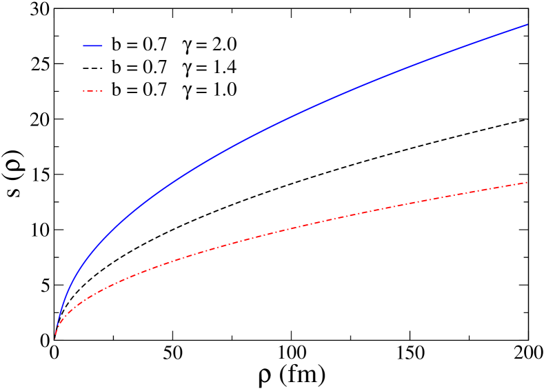
Figure 2: (Color online) Different LSTs with parameter $b=0$.$7$ fm and three values of $\gamma$: 2.0, 1.4, and 1.0 fm^1/2.

II.2 Hamiltonian matrix elements

The three-body Hamiltonian in hyperspherical coordinates is written as

$$\widehat{\mathcal{H}}(\rho,\Omega)=\widehat{T}(\rho,\Omega)+\widehat{V}(\rho,\Omega).$$ (9)

The kinetic energy operator is Nielsen01 ; MRoGa05

$$\widehat{T}(\rho,\Omega)=-\frac{\hbar^{2}}{2m}\left[\frac{\partial^{2}}{\partial\rho^{2}}+\frac{5}{\rho}\frac{\partial}{\partial\rho}-\frac{1}{\rho^{2}}\widehat{K}^{2}(\Omega)\right],$$ (10)

where $m$ is a normalization mass that we take as the nucleon mass and $\widehat{K}^{2}(\Omega)$ represents the hyperangular momentum or hypermomentum operator. $\widehat{T}(\Omega)$ does not connect different channels $\beta$ or states with different total angular momentum $j$. The Hamiltonian matrix elements have to be calculated between states given by Eq. (1), which separates the hyperradial and hyperangular parts. The hyperradial wave functions are constructed with Eq. (7) and satisfy the same normalization condition as the HO functions in six dimensions MRoGaTh ,

$$\int_{0}^{\infty}d\rho~{}\rho^{5}R_{i\beta}^{\text{THO}}(\rho)R_{i^{\prime}\beta}^{\text{THO}}(\rho)=\delta_{ii^{\prime}}.$$ (11)

For convenience, we introduce the hyperradial wave functions $U_{i\beta}^{\text{THO}}(\rho)$ as

$$U_{i\beta}^{\text{THO}}(\rho)=\rho^{5/2}R_{i\beta}^{\text{THO}}(\rho),$$ (12)

which satisfy the orthonormality relationship

$$\int_{0}^{\infty}d\rho~{}U_{i\beta}^{\text{THO}}(\rho)U_{i^{\prime}\beta}^{\text{THO}}(\rho)=\delta_{ii^{\prime}}.$$ (13)

With these functions, the kinetic energy operator can be re-written as

$$\widehat{T}_{U}(\rho)=-\frac{\hbar^{2}}{2m}\left[\frac{d^{2}}{d\rho^{2}}-\frac{15/4+K(K+4)}{\rho^{2}}\right]$$ (14)

and its matrix elements are JCasalMSc

$$\langle i\beta j|\widehat{T}(\rho,\Omega)|i^{\prime}\beta^{\prime}j\rangle=\langle i\beta j|\widehat{T}_{U}(\rho)|i^{\prime}\beta j\rangle~{}\delta_{\beta\beta^{\prime}}$$

$$=\delta_{\beta\beta^{\prime}}~{}\frac{\hbar^{2}}{2m}~{}\left[\int_{0}^{\infty}d\rho~{}\frac{dU_{i\beta}^{\text{THO}}(\rho)}{d\rho}~{}\frac{dU_{i^{\prime}\beta}^{\text{THO}}(\rho)}{d\rho}\right.$$

$$+\left(\frac{15}{4}+K(K+4)\right)\left.\int_{0}^{\infty}d\rho~{}U_{i\beta}^{\text{THO}}(\rho)\frac{1}{\rho^{2}}U_{i^{\prime}\beta}^{\text{THO}}(\rho)\right],$$

where the anti-hermiticity of the derivation operator has been taken into account.

The potential energy operator does connect, in general, different channels within the same $j$. The hyperangular integration is performed by using a set of subroutines from the code FaCE IJThompson04 that provides the hyperangular matrix elements $V_{\beta\beta^{\prime}}^{j}(\rho)$, depending on $\rho$. These functions are then integrated in the hyperradial variable, obtaining the potential energy matrix elements as

$$\langle i\beta j|\widehat{V}(\rho,\Omega)|i^{\prime}\beta^{\prime}j\rangle=$$

$$\int_{0}^{\infty}d\rho~{}U_{i\beta}^{\text{THO}}(\rho)V_{\beta\beta^{\prime}}^{j}(\rho)~{}U_{i^{\prime}\beta^{\prime}}^{\text{THO}}(\rho).$$ (16)

Once the kinetic energy and potential matrix elements are computed, the Hamiltonian is diagonalized in a truncated THO basis with $i_{\rm max}$ and the eigenstates of the system are obtained.

II.3 Transition probabilities $\boldsymbol{B(E\lambda)}$

As in Ref. MRoGa05 , we follow the notation of Brink and Satchler BrinkSatchler . The reduced transition probability between states of a system is defined as

$$B(E\lambda)_{nj,n^{\prime}j^{\prime}} \equiv B(E\lambda;nj\rightarrow n^{\prime}j^{\prime})$$ (17)

$$= |\langle nj\|\widehat{Q}_{\lambda}\|n^{\prime}j^{\prime}\rangle|^{2}\left(\frac{2\lambda+1}{4\pi}\right),$$

where $\widehat{Q}_{\lambda}$ is the electric multipole operator of order $\lambda$.

When a three-body system with only one charged particle, such as ⁶He (${}^{4}\text{He}+n+n$), is considered and the Jacobi system T illustrated in Fig. 1 is used, the operator $\widehat{Q}_{\lambda}$ reads as

$$Q_{\lambda M_{\lambda}}(\boldsymbol{y})=\left(\frac{4\pi}{2\lambda+1}\right)^{1/2}Z~{}e~{}\left(\frac{\sqrt{ma_{y}}}{m_{c}}\right)^{\lambda}y^{\lambda}Y_{\lambda M_{\lambda}}(\widehat{y}).$$ (18)

In this expression $Z$ is the atomic number of the system, $e$ is the electron charge, $m$ the mass of the nucleon, $a_{y}$ the reduced mass of the subsystem related by the Jacobi coordinate $\boldsymbol{y}$ and $m_{c}$ the mass of the charged particle (the core in the case of ⁶He). The reduced matrix elements of this operator can be expanded in terms of the THO basis obtaining the expression MRoGaTh ; MRoGa08

$$\langle nj\|\widehat{Q}_{\lambda}\|n^{\prime}j^{\prime}\rangle = (-1)^{j+2j^{\prime}}\text{ }\hat{j}^{\prime}Z\text{ }e\left(\frac{\sqrt{ma_{y}}}{m_{c}}\right)^{\lambda}$$

$$\times \sum_{\beta\beta^{\prime}}\delta_{l_{x}l_{x}^{\prime}}\delta_{S_{x}S_{x}^{\prime}}\delta_{jj_{ab}}\delta_{j^{\prime}j_{ab}^{\prime}}(-1)^{l_{x}+S_{x}}$$

$$\times \hat{l}_{y}\hat{l}_{y}^{\prime}\hat{l}\hat{l}^{\prime}W(ll^{\prime}l_{y}l_{y}^{\prime};\lambda l_{x})W(jj^{\prime}ll^{\prime};\lambda S_{x})$$

$$\times \begin{pmatrix}l_{y}&\lambda&l_{y}^{\prime}\\ 0&0&0\end{pmatrix}\sum_{ii^{\prime}}C_{n}^{i\beta j}C_{n^{\prime}}^{i^{\prime}\beta^{\prime}j^{\prime}}$$

$$\times \int\int d\alpha~{}d\rho~{}(\sin\alpha)^{2}(\cos\alpha)^{2}$$

$$\times U^{\text{THO}}_{i\beta}(\rho)\varphi^{l_{x}l_{y}}_{K}(\alpha)y^{\lambda}\varphi^{l_{x}l_{y}^{\prime}}_{K^{\prime}}(\alpha)U^{\text{THO}}_{i^{\prime}\beta^{\prime}}(\rho).$$

Since $n$ and $n^{\prime}$ enumerate the different eigenstates, transition probabilities given by Eq. (17) are a set of discrete values. In order to obtain continuous energy distributions from discrete values, the best option is to do the overlap with the continuum wave functions MRoGa11 , if they are known. In this case the smoothed THO $B(E1)$ distribution must coincide perfectly with the actual continuum $B(E1)$ distribution. When the continuum states are not available, it is considered that, in general, a PS with energy $\varepsilon_{n}$ is the superposition of continuum states in the vicinity. There are several ways to assign an energy distribution to a PS PDes12 ; Macias87 . In this work, for each discrete value of $B(E\lambda)(\varepsilon_{n})$, a Poisson distribution $D(\varepsilon,\varepsilon_{n},w)$ with the following form is assigned,

$$D(\varepsilon,\varepsilon_{n},w)=\frac{(w+1)^{(w+1)}}{\varepsilon_{n}^{w+1}\Gamma(w+1)}\varepsilon^{w}\exp{\left(-\frac{w+1}{\varepsilon_{n}}\varepsilon\right)},$$ (20)

which is properly normalized. The parameter $w$ controls the width of the distributions; as $w$ decreases, the width of the distributions increases. Finally, the $B(E\lambda)$ distribution is given by the expression

$$\frac{dB(E\lambda)}{d\varepsilon}(\varepsilon,w)=\sum_{n}D(\varepsilon,\varepsilon_{n},w)~{}B(E\lambda)(\varepsilon_{n}).$$ (21)

The $B(E1)$ distribution so obtained can be compared easily in the case of ⁶He with the continuum distribution in order to check the smoothing procedure.

One can also calculate the sum rules for electric transitions from the ground state (g.s.) to the states $(n,j)$ in order to test the completeness of the basis used. Using the Eq. (17)

$$\sum_{n}B(E\lambda)_{\text{g.s.},nj}=\left(\frac{2\lambda+1}{4\pi}\right)\sum_{n}|\langle\text{g.s.}\|\widehat{Q}_{\lambda}\|nj\rangle|^{2},$$ (22)

a closed expression is obtained

$$\sum_{n}B(E\lambda)_{\text{g.s.},nj}=\frac{2\lambda+1}{4\pi}\frac{Z^{2}e^{2}m^{\lambda}a_{y}^{\lambda}}{m_{c}^{2\lambda}}\langle\text{g.s.}|y^{2\lambda}|\text{g.s.}\rangle.$$ (23)

III Radiative capture reaction rate

The formalism introduced above allows calculations of astrophysical interest. As stated in the introduction, some Borromean nuclei are important in the nucleosynthesis processes, and an accurate knowledge of their reaction and production rates in different scenarios is essential to understand the origin of the different elements in the Universe. We focus on radiative capture reactions of three particles, ($abc$), into a bound nucleus $A$ of binding energy $|\varepsilon_{B}|$, i.e., $a+b+c\rightarrow$ $A+\gamma$. The energy-averaged reaction rate for such process, $\langle R_{abc}(\varepsilon)\rangle$, is given as a function of the temperature $T$ by the expression Garrido11

$$\langle R_{abc}(\varepsilon)\rangle(T)=\int R_{abc}(\varepsilon)F_{B}(\varepsilon,T)d\varepsilon.$$ (24)

The function $F_{B}(\varepsilon,T)$ is the Maxwell-Boltzmann distribution and $R_{abc}(\varepsilon)$ is the radiative capture reaction rate at a certain excitation energy $\varepsilon$. It can be obtained from the inverse photodissociation process RdDiego10 ; Garrido11 and is given by the expression

$$R_{abc}(\varepsilon)=\nu!\frac{\hbar^{3}}{c^{2}}\frac{8\pi}{(a_{x}a_{y})^{3/2}}\left(\frac{\varepsilon_{\gamma}}{\varepsilon}\right)^{2}\frac{2g_{A}}{g_{a}g_{b}g_{c}}\sigma_{\gamma}(\varepsilon_{\gamma}),$$ (25)

where $\varepsilon=\varepsilon_{\gamma}+\varepsilon_{B}$ is the initial three-body kinetic energy, $\varepsilon_{\gamma}$ is the energy of the photon emitted, $\varepsilon_{B}$ is the ground-state energy, $g_{i}$ are the spin degeneracy of the particles, $\nu$ is the number of identical particles in the three-body system, and $a_{x}$ and $a_{y}$ are the reduced masses of the subsystems related to the Jacobi coordinates $\{\boldsymbol{x},\boldsymbol{y}\}$. The photodissociation cross section $\sigma_{\gamma}(\varepsilon_{\gamma})$ of the nucleus $A$ can be expanded into electric and magnetic multipoles RdDiego10 ; Forseen03

$$\sigma_{\gamma}^{(\mathcal{O}\lambda)}(\varepsilon_{\gamma})=\frac{(2\pi)^{3}(\lambda+1)}{\lambda[(2\lambda+1)!!]^{2}}\left(\frac{\varepsilon_{\gamma}}{\hbar c}\right)^{2\lambda-1}\frac{dB(\mathcal{O}\lambda)}{d\varepsilon},$$ (26)

which are related to the transition probability distributions $dB(\mathcal{O}\lambda)/d\varepsilon$, for $\mathcal{O}=E,M$.

From Eqs. (24) and (25), we write the energy-averaged capture reaction rate expression for the contribution of order $\lambda$ as

$$\langle R_{abc}(\varepsilon)\rangle(T)= ~{}\nu!\frac{\hbar^{3}}{c^{2}}\frac{8\pi}{(a_{x}a_{y})^{3/2}}\frac{g_{A}}{g_{a}g_{b}g_{c}}\frac{1}{(k_{B}T)^{3}}$$

$$\times \int_{0}^{\infty}(\varepsilon+|\varepsilon_{B}|)^{2}\sigma_{\gamma}^{(\mathcal{O}\lambda)}(\varepsilon+|\varepsilon_{B}|)e^{\frac{-\varepsilon}{k_{B}T}}d\varepsilon.$$ (27)

This integral is very sensitive to the $dB(\mathcal{O}\lambda)/d\varepsilon$ behavior at low energy and, for that reason, a detailed description of the transition probability distribution in that region is needed to avoid numerical errors. Accordingly to the traditional literature Weiss , in absence of low energy resonances, the first multipole contribution is the dominant one and the electric contribution dominates over the magnetic one at the same order.

IV Application to ⁶He

The ⁶He nucleus can be explained as a three-body system, formed by an inert $\alpha$ core and two valence neutrons. This is the simplest case to test the formalism developed in this work since there is just one charged particle and the three-body continuum wave functions can be generated easily. Comparison with actual continuum wave functions may serve as a reference for any other calculation. In addition, valuable experimental information is available on the ground state: total angular momentum $j^{\pi}=0^{+}$, experimental binding energy of 0.975 MeV Brouder12 , and rms point nucleon matter radius within 2.5$-$2.6 fm Danilin05 . It has also a well-known $2^{+}$ resonance at 0.824 MeV over the breakup threshold.

To describe ⁶He, we use a model Hamiltonian that includes the two-body $n$-$n$ and $\alpha$-$n$ potentials, and also a simple central hyperradial three-body force. These potentials are those used in Ref. MRoGa05 ; the $n$-$\alpha$ potential taken from Refs. Bang79 ; IJThompson00 , with central and spin-orbit components, and the GPT $n$-$n$ potential GPT with central, spin-orbit, and tensor components. These two-body potentials are kept fixed for any total angular momentum and parity $j^{\pi}$. However, this Hamiltonian does not include all possible potential contributions. To include them effectively, a three-body force is usually introduced. In this work we have used the simple power form

$$V_{3b}(\rho)=\frac{v_{3b}}{1+\left(\frac{\rho}{r_{3b}}\right)^{a_{3b}}}.$$ (28)

The parameters $v_{3b}$, $r_{3b}$, and $a_{3b}$ have been chosen to adjust the energy of the $0^{+}$ ground state and the position of the known $2^{+}$ resonance to the experimental values.

In three-body models of halo nuclei, such as ⁶He, the Pauli principle treatment is important to block occupied core states to the valence neutrons. That is, Pauli blocking is needed to remove forbidden states, which would disappear under antisymmetrization. This can be taken into account by several methods. In this work, a “repulsive core” in the $s$-wave component of the $\alpha$-$n$ subsystem is introduced with the requirement that the experimental phase shifts are correctly calculated. This method is referred in the literature as the PC method IJThompson00 .

The radiative capture of two neutrons by an alpha particle producing ⁶He is dominated by a dipolar process from the $1^{-}$ continuum of ⁶He to the $0^{+}$ ground state RdDiego10 . For ⁶He, low-energy dipolar resonances have not been observed, then the electric dipole dominates over the magnetic dipole. A low-energy quadrupole resonance does exist (as mentioned above). We have calculated both dipolar and quadrupolar electric contributions, concluding the quadrupole is several orders of magnitude lower than the dipole. This means that the reaction rate for this capture process is mainly governed by the dipolar electric transition distribution $dB(E1)/d\varepsilon$ of ⁶He. Then, to compute this distribution we need to generate the THO basis for states $0^{+}$ and $1^{-}$. The $0^{+}$ THO basis must provide a well-converged ground state. The $1^{-}$ THO basis must have enough states close to the break-up threshold to get a smooth and detailed $B(E1)$ distribution in that region. Using the parameters $b$ and $\gamma$ from the analytical LST one can find the most suitable THO basis for each total angular momentum ($0^{+}$ and $1^{-}$). The THO bases were truncated at maximum hypermomentum $K_{max}=20$, as it was sufficient to have a good description of the system and provide converged results.

IV.1 States $j^{\pi}=0^{+}$

The $0^{+}$ states are described with an analytical THO basis defined by parameters $b=0.7$ fm and $\gamma=1.4$ fm^1/2, trying to minimize the size of the basis needed to reach convergence of the ground state. We found that a basis with larger $\gamma/b$ has a too large energy distribution to provide a fast convergence for the ground state. On the other hand, a basis with smaller $\gamma/b$ has a very large hyperradial extension and does not describe properly the interior region of the potential where the ground state probability is larger. The three-body force parameters are taken as $v_{3b}=-2.45$ MeV, $r_{3b}=5$ fm, and $a_{3b}=3$ in order to adjust both, the ground-state energy and the matter radius of ⁶He.

In Fig. 3 we show the first THO hyperradial wave functions for the channel $\beta\equiv\{2,0,0,0,0,0\}$, using the given LST and three-body force parameters. This channel is the most important ground-state channel, with a 78.6% contribution to the total norm. We can see in the figure that as $i$ increases, the functions are more oscillatory and explore larger distances.

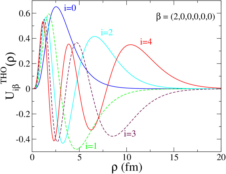
Figure 3: (Color online) First five THO hyperradial wave functions for the channel $\beta\equiv\{2,0,0,0,0,0\}$, the most important channel in the g.s. wave function.

In Fig. 4 the Hamiltonian eigenvalues for $j^{\pi}=0^{+}$, for an increasing number of hyperradial excitations, $i_{\rm max}$, are presented up to 10 MeV. The calculated ground-state is stable, has a binding energy of 0.9749 MeV and a rms point nucleon matter radius of 2.554 fm. Calculations assume an $\alpha$ radius of 1.47 fm. In Table I the ground-state energy $\varepsilon_{B}$ and matter radius $r_{mat}$ are shown as a function of the maximum number of hyperradial excitations $i_{\rm max}$. We observe a fast convergence of this two ground-state observables within this THO basis.

Figure 4: Eigenvalues for $j^{\pi}=0^{+}$ up to 10 MeV.

$i_{\rm max}$	$\varepsilon_{B}$ (MeV)	$r_{mat}$ (fm)
5	$-$0.9452	2.511
10	$-$0.9744	2.552
15	$-$0.9748	2.554
20	$-$0.9749	2.554
25	$-$0.9749	2.554

Table 1: Ground-state energy $\varepsilon_{B}$ and matter radius $r_{mat}$ as a function of $i_{\rm max}$. A fast convergence is observed.

The first three hyperradial components of the ground-state wave function for $i_{\rm max}=25$ are presented in Fig. 5. The curves match a reference calculation of the ground-state wave function corresponding to the same model Hamiltonian. By reference calculation we mean the procedure presented in Ref.  IJThompson00 and implemented in the codes FaCE IJThompson04 and sturmxx sturmxx , using a suitable basis for bound states, the so-called Sturmian basis.

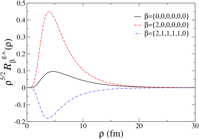
Figure 5: (Color online) Hyper-radial wave function, $\mathcal{R}_{\beta}^{\text{g.s.}}(\rho)$, for the first three channels included in the ground state of ⁶He.

Once the $0^{+}$ ground state is obtained, the $1^{-}$ states in the continuum have to be generated. However, no reference is available to fix the $1^{-}$ three-body force. For the $2^{+}$ continuum states there is a resonance experimentally observed at 0.824 MeV over the breakup threshold. Thus, usually the three-body force is fixed to set the $2^{+}$ resonance at the experimental value and it is accepted the same three-body force for the $1^{-}$ states. So we generate first the THO basis for 2⁺ states and adjust the position of the $2^{+}$ resonance by using a particular three-body force. Then we use the same force for the $1^{-}$ states.

IV.2 $\boldsymbol{2^{+}}$ states

The $2^{+}$ states were described with a basis defined by $b=0.7$ fm and $\gamma=2.0$ fm^1/2. This basis has a small hyperradial extension and spreads the eigenvalues obtained upon diagonalization at higher energies. This choice allows us to have only one pseudo-state presenting the characteristics of the resonance, since the rest of states are sufficiently above the resonance energy position for medium-size bases. In this way we can adjust the resonance energy, setting the energy of this state to the experimental value. Then, the three-body force parameters are taken as $v_{3b}=-0.90$ MeV, $r_{3b}=5$ fm, and $a_{3b}=3$.

Figure 6: Eigenvalues for $j^{\pi}=2^{+}$ up to 10 MeV.

In Fig. 6, the eigenvalues of the Hamiltonian for $j^{\pi}=2^{+}$ states, for an increasing number of hyperradial excitations, are shown. The lowest state is rather stable and close to the energy of the known $2^{+}$ resonance, 0.824 MeV. In Fig. 7, we present the probability density for this first $2^{+}$state, compared with the $0^{+}$ ground state probability. The contributions of the three most important channels for each one are shown. We can see the PS representing the resonance is a state with a large probability in the interior part, similar to a bound state.

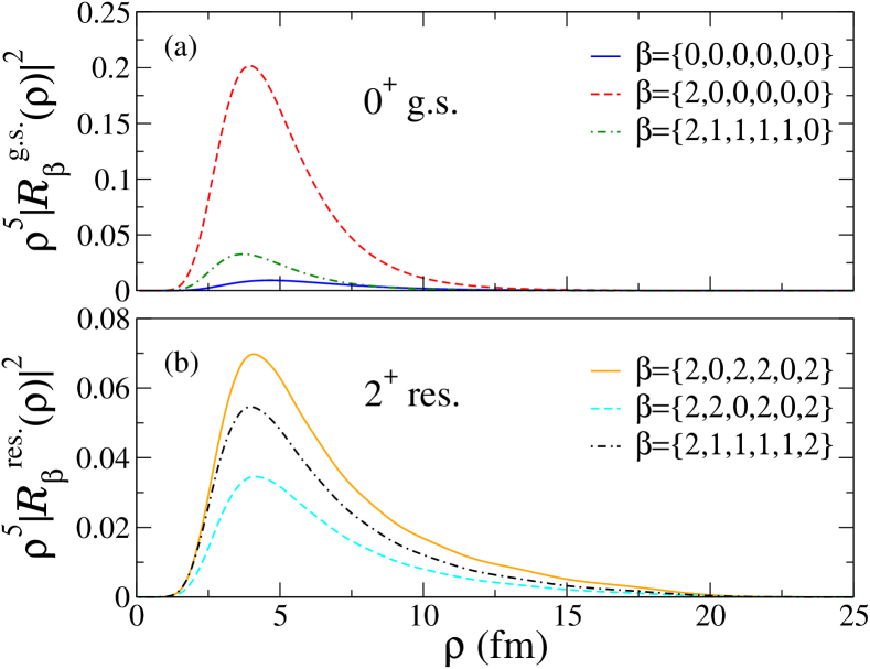
Figure 7: (Color online) Ground-state (a) and resonance state (b) probabilities.

IV.3 $\boldsymbol{1^{-}}$ states

The preceding calculation on $2^{+}$ states with the low-lying resonance as reference allows us to select the three-body force ($v_{3b}=-0.90$ MeV, $r_{3b}=5$ fm, $a_{3b}=3$) to be included in the calculation of the required $1^{-}$ states.

To get a well-defined $B(E1)$ distribution near the origin, we need, for $1^{-}$ states, a basis which has a large hyperradial extension to concentrate many eigenvalues close to the breakup threshold. For this purpose we use a THO basis with $b=0.7$ fm and $\gamma=1.0$ fm^1/2. The eigenvalues of the Hamiltonian for $j^{\pi}=1^{-}$ states are presented for different $i_{\rm max}$ values in Fig. 8. If we compare this $1^{-}$ spectrum with the $0^{+}$ and $2^{+}$ spectra for a fixed $i_{\rm max}$, it is clear the difference in eigenstates density depending on the extension of the basis, that is, depending on the LST parameters $b$ and $\gamma$.

Figure 8: Eigenvalues for $j^{\pi}=1^{-}$ up to 10 MeV.

Next we can calculate the discrete transition probabilities $B(E1)$ from the $0^{+}$ ground state to the $1^{-}$ eigenstates. We have first checked the completeness of the basis for a given $i_{\rm max}$ comparing the sum of the discrete $B(E1)$ transition probabilities with the sum rule Eq. (23). This is given in Table II. The summation converges to the exact value given by the sum rule, 1.493 e²fm².

$i_{\rm max}$		$\sum B(E1)$ (e2fm2)
5		1.402
10		1.489
15		1.492
20		1.492
25		1.493
30		1.493
35		1.493

Table 2: Sum of $B(E1)$ as a function of $i_{\rm max}$.

For the evaluation of the transition probabilities, we use a THO basis with $i_{\rm max}=35$ in order to obtain a detailed behavior for the low energy part of the $B(E1)$ distribution. In Fig. 9 we show, up to 6 MeV, a reference calculation obtained by using the actual three-body continuum wave functions which, in this simple case, can be computed easily IJThompson00 (dash red line). To generate the continuum wave functions we have used the codes FaCE IJThompson04 and sturmxx sturmxx with the same model Hamiltonian. If the smoothing of our THO calculation is done using the overlap with the continuum wave functions, the obtained $B(E1)$ distribution is indistinguishable from the reference one. This guarantees that the formalism presented here is working correctly. However, since our interest is to extend this formalism to other systems for which the true continuum wave functions are difficult to obtain, we propose an alternative smoothing procedure following Eqs. (20) and (21). In Fig. 9 the THO distribution for $B(E1)$, using this alternative smoothing, is shown (full black line). We have used Poisson distributions with parameter $w=30\sqrt{\varepsilon_{n}}$, such that it ensures a smooth $B(E1)$ distribution without spreading it unphysically. Due to the large number of basis states we have near the threshold, the energy dependence of $w$ is convenient to produce a smooth distribution in that region. The total $B(E1)$ strength is the same for both calculations (solid and dashed lines) and the behavior is similar, although small differences are observed in the medium energy range.

It is also included in Fig. 9 a calculation taken from Ref. RdDiegoTh . In that work, the hyperspherical adiabatic expansion method is used instead of the HH method. Then, the three-body states are calculated by box boundary conditions, obtaining a discrete spectrum. The discrete $B(E1)$ values are smoothed using the finite energy interval approximation. This calculation clearly have a different behavior at low energies. The difference comes from the difficulty to have a large energy level density at low energies solving the problem in a box. It is also apparent that the total $B(E1)$ from this calculation is considerably lower than ours. In our calculation the smoothed $B(E1)$ energy distribution is very well-defined close to the break-up threshold since we have been able, using the analytical THO, to build a basis for $1^{-}$ states concentrating many eigenvalues close to the breakup threshold. In the literature, one can find other $B(E1)$ distributions for ⁶He using different three-body formalisms. We would like to cite Myo01 and Baye09 , globally both compare reasonably well with our results but have not been included in Fig. 9 since it is not possible to extract from the plots presented in those publications the detailed behavior at low energies. Without this information, one cannot calculate converged reaction rates below 1–2 GK.

It is worth mentioning that the available experimental data Aumann99 (not shown in Fig. 9) differ significantly from all published theoretical calculations. In particular the data do not show the enhancement at energies around 1 MeV. Either new experiment or reanalysis of the existing data is clearly needed.

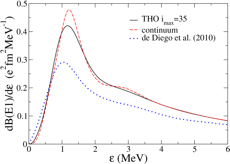
Figure 9: (Color online) $B(E1)$ distribution up to 6 MeV: this work (full black line), a calculation using the actual continuum wave functions, that in this case can be calculated, (broken red line), and Ref. RdDiegoTh (dotted blue line).

In order to show the convergence of calculations with $K_{\rm max}$ and that $K_{\rm max}=20$ is sufficient to provide converged results, we present in Fig. 10 the $B(E1)$ distribution for different $K_{\rm max}$ values. In these calculations the same two- and three-body forces are kept fixed. It is clear from the figure that the calculations for $K_{\rm max}=20$, 22, and 24 are very close together.

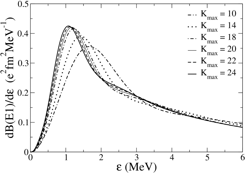
Figure 10: $B(E1)$ distribution up to 6 MeV as $K_{\rm max}$ increases.

Once obtained the $B(E1)$ energy distribution, we can finally calculate the reaction rate (Eq. (27)) for the radiative capture reaction $\alpha+n+n\to~{}^{6}\text{He}+\gamma$. In Fig. 11, we present the result for the low temperature region of astrophysical interest (0-5 GK). Our calculation is the full black line. In the same figure the reaction rate obtained using the actual three-body continuum wave functions and the corresponding $B(E1)$ is represented with a dash red line. The dotted blue line is the calculation of Ref. RdDiegoTh . We can see from the figure that our calculation agrees very well with the reference calculation for low and high temperatures. In the region between 0.1 and 1.5 GK, there are differences at most by a 3 or 4 factor. These differences with respect to the reference (red dashed line) calculation are more than one order of magnitude in the same temperature region for the calculation of Ref. RdDiegoTh . This is due to the already referred different behavior of the corresponding $B(E1)$ distributions at low energies (below 0.5 MeV). We have checked that this region is crucial for the computation of the reaction rates, especially at low temperatures (below 1–1.5 GK). We have also checked that small differences in the $B(E1)$ distributions between 0.5 and 3.5 MeV do not affect the calculated reaction rate provided the same total strength.

In Fig. 11, we have also included the results from a sequential model for the radiative capture Bartlett06 (dot-dashed orange). This calculation presents the same behavior as ours but is a factor of two larger above 0.2 GK. It is worth mentioning that this sequential calculation assumes first the formation of a dineutron, which is controversial, and then the capture of this by an $\alpha$ particle. An alternative sequential process, presented also in Ref. Bartlett06 , starts from a neutron capture by the $\alpha$ particle to give ⁵He followed by the capture of a second neutron. This provides a reaction rate more than two orders of magnitude smaller in all studied ranges of temperatures.

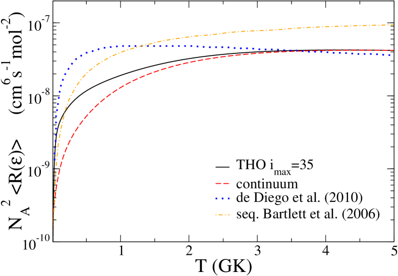
Figure 11: (Color online) Reaction rate for the radiative capture $\alpha+n+n\to^{6}\text{He}+\gamma$ with different models: this work (full black line), a reference calculation using the actual three-body continuum wave functions (dash red line), the results from Ref. RdDiegoTh (dotted blue line), and the results from a sequential calculation  Bartlett06 (dot-dashed orange line).

We would like to stress our calculation is based on a full three-body model that makes no assumptions about the reaction mechanism. In this sense all the physical sequential processes are implicitly included.

V Summary and conclusions

We have extended the analytical THO method for the study of three-body systems. There are several advantages of the analytical over the numerical THO method: (1) The previous knowledge of the ground-state of the system is not needed. (2) The analytical transformation is easy to be implemented in programming languages. (3) The versatility of the LST depending on the parameters $b$ and $\gamma$, allows one to design the best basis for the observable under study.

We have applied the formalism to the well-known Borromean nucleus ⁶He. This nucleus can be described as an $\alpha$ particle and two valence neutrons. We have seen that the use of the analytical THO method allows a specific basis selection depending on the needs for each angular momentum of the system and on the observable under study. We have calculated a well-converged $0^{+}$ ground state and a rather stable $2^{+}$ resonant state. For $1^{-}$ states we have chosen a basis concentrating many energy levels close to the breakup threshold in order to have a fine description for that region.

With these ingredients we have computed the $B(E1)$ transition probabilities from the $0^{+}$ ground state to the $1^{-}$ states. We have checked that the smoothing, using the overlap with the actual continuum wave functions, produce the same $B(E1)$. The smoothing using Poisson distributions produces a similar result with small differences in the medium-energy region. In this case, the obtained $B(E1)$ distribution is well-defined at low energies (below 0.5 MeV), which is crucial to estimate properly observables such as the reaction rate of the radiative capture $\alpha+n+n\to~{}^{6}\text{He}+\gamma$.

We have calculated the reaction rate of the radiative capture $\alpha+n+n\to~{}^{6}\text{He}+\gamma$ from the $B(E1)$ distribution for temperatures of astrophysical interest. The result with Poisson smoothing for the $B(E1)$ provides a reasonable approach to the continuum reaction rate. However it differs by a factor of 2 from the sequential mechanism presented in Ref. Bartlett06 , which assumes the dineutron preformation, what is controversial. The differences with the reaction rate calculated in Ref. RdDiegoTh , using also a full three-body model, come from the different behaviors at low energies of the $B(E1)$ distributions (below 0.5 MeV) and the different total $B(E1)$ strengths.

The present results encourage the application of this formalism to more interesting astrophysical cases, such as ⁹Be, the triple-$\alpha$ process to produce ¹²C, or ¹⁷Ne. In the study of these systems, one of the major problems is the proper treatment of the Coulomb interaction at large distances. However, this problem is absent in the PS methods, such as the analytical THO presented here.

- (1) M. V. Zhukov, B. V. Danilin, D. V. Fedorov, J. M. Bang, I. J. Thompson, and J. S. Vaagen, Phys. Rep. 231, 151 (1993)
- (2) F. Hoyle, Astrophys. J. Supp. Ser. 1, 121 (1954)
- (3) A. Aprahamian, K. Langanke, and M. Wiescher, Prog. Part. Nucl. Phys. 54, 535 (2005)
- (4) N. B. Nguyen, F. M. Nunes, I. J. Thompson, and E. F. Brown, Phys. Rev. Lett. 109, 141101 (2012)
- (5) V. D. Efros, W. Balogh, H. Herndl, R. Hofinger, and H. Oberhummer, Z. Phys. A 355, 101 (1996)
- (6) K. Sumiyoshi, H. Utsunomiya, S. Goko, and T. Kajino, Nucl. Phys. A 709, 467 (2002)
- (7) A. Bartlett, J. Görres, G. J. Mathews, K. Otsuki, M. Wiescher, D. Frekers, A. Mengoni, and J. Tostevin, Phys. Rev. C 74, 015802 (2006)
- (8) B. S. Meyer, G. J. Mathews, W. M. Howard, S. E. Woosley, and R. D. Hoffman, Astrophys. J. 399, 656 (1992)
- (9) B. S. Meyer, Annu. Rev. Astron. Astrophys. 32, 153 (1994)
- (10) P. G. Hansen, A. S. Jensen, and B. Jonson, Annu. Rev. Nucl. Part. Sci. 45, 591 (1995)
- (11) J. A. Lay, A. M. Moro, J. M. Arias, and J. Gómez-Camacho, Phys. Rev. C 82, 024605 (2010)
- (12) Y. C. Tang and D. R. Thompson, Phys. Rep. 47, 167 (1978)
- (13) V. D. Efros, W. Leidemann, and G. Orlandini, Phys. Lett. B 338, 130 (1994)
- (14) S. Bacca, M. A. Marchisio, N. Barnea, W. Leidemann, and G. Orlandini, Phys. Rev. Lett. 89, 052502 (2002)
- (15) E. P. Wigner and L. Eisenbud, Phys. Rev. 72, 29 (1947)
- (16) I. J. Thompson, B. V. Danilin, V. D. Efros, J. S. Vaagen, J. M. Bang, and M. V. Zhukov, Phys. Rev. C 61, 024318 (2000)
- (17) P. Descouvemont, E. Tursunov, and D. Baye, Nucl. Phys. A 765, 370 (2006)
- (18) R. de Diego, E. Garrido, D. V. Fedorov, and A. S. Jensen, Eur. Phys. Lett. 90, 52001 (2010)
- (19) N. Austern, Y. Iseri, M. Kamimura, M. Kawai, G. Rawitsher, and M. Yahiro, Phys. Rep. 154, 125 (1987)
- (20) A. U. Hazi and H. S. Taylor, Phys. Rev. A 1, 1109 (1970)
- (21) T. Matsumoto, T. Kamizato, K. Ogata, Y. Iseri, E. Hiyama, M. Kamimura, and M. Yahiro, Phys. Rev. C 68, 064607 (2003)
- (22) M. Rodríguez-Gallardo, J. M. Arias, and J. Gómez-Camacho, Phys. Rev. C 69, 034308 (2004)
- (23) A. M. Moro, J. M. Arias, J. Gómez-Camacho, and F. Pérez-Bernal, Phys. Rev. C 80, 054605 (2009)
- (24) T. Matsumoto, E. Hiyama, M. Yahiro, K.Ogata, Y. Iseri, and M. Kamimura, Nucl. Phys. A 738, 471 (2004)
- (25) R. Y. Rasoanaivo and G. H. Rawitscher, Phys. Rev. C 39, 1709 (1989)
- (26) M. Rodríguez-Gallardo, J. M. Arias, J. Gómez-Camacho, A. M. Moro, I. J. Thompson, and J. A. Tostevin, Phys. Rev. C 72, 024007 (2005)
- (27) F. Pérez-Bernal, I. Martel, J. M. Arias, and J. Gómez-Camacho, Phys. Rev. A 63, 052111 (2001)
- (28) A. M. Moro, J. M. Arias, J. Gómez-Camacho, I. Martel, F. Pérez-Bernal, R. Crespo, and F. Nunes, Phys. Rev. C 65, 011602(R) (2001)
- (29) A. M. Moro, F. Pérez-Bernal, J. M. Arias, and J. Gómez-Camacho, Phys. Rev. C 73, 044612 (2006)
- (30) M. Rodríguez-Gallardo, J. M. Arias, J. Gómez-Camacho, R. C. Johnson, A. M. Moro, I. J. Thompson, and J. A. Tostevin, Phys. Rev. C 77, 064609 (2008)
- (31) S. Karataglidis, K. Amos, and B. G. Giraud, Phys. Rev. C 71, 064601 (2005)
- (32) F. Aksough et al., Ricerca Scientifica ed Educazione Permanente Suppl. 122, 157 (2003)
- (33) P. Egelhof, Nucl. Phys. A 722, C254 (2003)
- (34) T. Aumann, L. V. Chulkov, V. N. Pribora, and M. H. Smedberg, Nucl. Phys. A 640, 24 (1998)
- (35) T. Aumann et al., Phys. Rev. C 59, 1252 (1999)
- (36) E. F. Aguilera et al., Phys. Rev. C 63, 061603(R) (2001)
- (37) E. F. Aguilera et al., Phys. Rev. Lett. 84, 5058 (2000)
- (38) O. R. Kakuee et al., Nucl. Phys. A 728, 339 (2003)
- (39) M. Rodríguez-Gallardo, Descripción del continuo en una base discreta: estructura del núcleo 6He y las reacciones que induce (ISBN: 978-84-692-6177-4), Ph.D. thesis, Universidad de Sevilla (2005), http://fondosdigitales.us.es/tesis/autores/953
- (40) E. Nielsen, D. V. Fedorov, A. S. Jensen, and E. Garrido, Phys. Rep. 347, 373 (2001)
- (41) J. Casal, Sistemas de tres cuerpos de interés en astrofísica: el caso de 6He, Master’s project, Universidad de Sevilla (2012)
- (42) I. J. Thompson, F. M. Nunes, and B. V. Danilin, Comput. Phys. Commun. 161, 87 (2004)
- (43) D. M. Brink and G. R. Satchler, Angular Momentum (Clarendon, Oxford, 1994)
- (44) M. Rodríguez-Gallardo and A. M. Moro, Int. J. Mod. Phys. E 20, 947 (2011)
- (45) P. Descouvemont, E. Pinilla, and D. Baye, Prog. Theor. Phys. Suppl. 196, 1 (2012)
- (46) A. Macías, F. Martín, A. Riera, and M. Yañez, Phys. Rev. A 36, 4179 (1987)
- (47) E. Garrido, R. de Diego, D. V. Fedorov, and A. S. Jensen, Eur. Phys. J. A 47, 102 (2011)
- (48) C. Forssén, N. B. Shul’gina, and M. V. Zhukov, Phys. Rev. C 67, 045801 (2003)
- (49) J. M. Blatt and V. F. Weisskopf, Theoretical Nuclear Physics (John Wiley and Sons, Inc., New York, 1966)
- (50) M. Brodeur, T. Brunner, C. Champagne, S. Ettenauer, M. J. Smith, A. Lapierre, R. Ringle, V. L. Ryjkov, S. Bacca, P. Delheij, G. W. F. Drake, D. Lunney, A. Schwenk, and J. Dilling, Phys. Rev. Lett. 108, 052504 (2012)
- (51) B. V. Danilin, S. N. Ershov, and J. S. Vaagen, Phys. Rev. C 71, 057301 (2005)
- (52) J. Bang and C. Gignoux, Nucl. Phys. A 313, 119 (1979)
- (53) D. Gogny, P. Pires, and R. De Tourreil, Phys. Lett. B 32, 591 (1970)
- (54) I. J. Thompson, Program sturmxx, available from: http://www.fresco.org.uk/programs/sturmxx/index.html
- (55) R. de Diego, Sistemas de tres cuerpos en el continuo y reacciones de interés astrofísico, Ph.D. thesis, Instituto de Estructura de la Materia, CSIC (2010)
- (56) T. Myo, K. Kato, S. Aoyama, and K. Ikeda, Phys. Rev. C 63, 054313 (2001)
- (57) D. Baye, P. Capel, P. Descouvemont, and Y. Suzuki, Phys. Rev. C 79, 024607 (2009)