Hydrodynamic limit in a particle system
with topological interactions

Abstract

We study a system of particles in the interval $[0,{\epsilon}^{-1}]\cap\mathbb{Z}$, ${\epsilon}^{-1}$ a positive integer. The particles move as symmetric independent random walks (with reflections at the endpoints); simultaneously new particles are injected at site $0$ at rate $j{\epsilon}$ ($j>0$) and removed at same rate from the rightmost occupied site. The removal mechanism is therefore of topological rather than metric nature. The determination of the rightmost occupied site requires a knowledge of the entire configuration and prevents from using correlation functions techniques.

We prove using stochastic inequalities that the system has a hydrodynamic limit, namely that under suitable assumptions on the initial configurations, the law of the density fields ${\epsilon}\sum\phi({\epsilon}x)\xi_{{\epsilon}^{-2}t}(x)$ ($\phi$ a test function, $\xi_{t}(x)$ the number of particles at site $x$ at time $t$) concentrates in the limit ${\epsilon}\to 0$ on the deterministic value $\int\phi\rho_{t}$, $\rho_{t}$ interpreted as the limit density at time $t$. We characterize the limit $\rho_{t}$ as a weak solution in terms of barriers of a limit free boundary problem.

1 Introduction and model definition

This paper is inspired by the analysis in [12] and we are indebted to Pablo Ferrari for discussions and in particular for suggesting the inequalities in Section 6. This is a first in a series of three papers where we study a particle system whose hydrodynamic limit is described by a free boundary problem.

Our system is made of particles confined to the lattice $[0,{\epsilon}^{-1}]\cap\mathbb{Z}$, for brevity in the sequel we shall just write $[0,{\epsilon}^{-1}]$. In this notation ${\epsilon}^{-1}$ is a positive integer denoting the system size and we will be eventually interested in the asymptotics as ${\epsilon}\to 0$. The evolution is a Markov process $\{\xi_{t},t\geq 0\}$ on the space of particles configurations $\xi=(\xi(x))_{x\in[0,{\epsilon}^{-1}]}$, the component $\xi(x)\in\mathbb{N}$ is interpreted as the number of particles at site $x$. The generator is denoted by

$$L=L^{0}+L_{b}+L_{a}$$ (1.1)

(the dependence on ${\epsilon}$ is not made explicit). $L^{0}$ is the generator of the independent random walks process, it is defined on functions $f$ by

$$L^{0}f(\xi)=\frac{1}{2}\sum_{x=0}^{{\epsilon}^{-1}-1}L^{0}_{x,x+1}f(\xi)$$ (1.2)

$$L^{0}_{x,x+1}f(\xi)=\xi(x)\left(f(\xi^{x,x+1})-f(\xi)\right)+\xi(x+1)\left(f(\xi^{x+1,x})-f(\xi)\right)$$ (1.3)

where $\xi^{x,y}$ denotes the configuration obtained from $\xi$ by removing one particle from site $x$ and putting it at site $y$, i.e.

$$\xi^{x,y}(z)=\left\{\begin{array}[]{ll}\xi(z)&\text{if }z\neq x,y,\\ \xi(z)-1&\text{if }z=x,\\ \xi(z)+1&\text{if }z=y.\end{array}\right.$$

Namely $L^{0}$ describes independent symmetric random walks which jump with equal probability after an exponential time of mean 1 to the nearest neighbor sites, the jumps leading outside $[0,{\epsilon}^{-1}]$ being suppressed (reflecting boundary conditions).

The term $L_{b}$ in (1.1) is

$$L_{b}f(\xi)=j{\epsilon}\left(f(\xi^{+})-f(\xi)\right),\quad\xi^{+}(x)=\xi(x)+\mathbf{1}_{x=0}$$ (1.4)

It describes the action of throwing into the system new particles at rate ${\epsilon}j$, $j>0$, which then land at site 0; instead $L_{a}$ removes particles:

$$L_{a}f(\xi)=j{\epsilon}\left(f(\xi^{-})-f(\xi)\right),\quad\xi^{-}(x)=\xi(x)-\mathbf{1}_{x=R(\xi)}$$ (1.5)

namely a particle is taken out from the edge $R_{\xi}$ of the configuration $\xi$ defined as

$$\text{ $R_{\xi}$ is such that:}\;\;\;\begin{cases}\xi(y)>0&\text{for $y=R_{\xi}$}\\ \xi(y)=0&\text{for $y>R_{\xi}$}\end{cases}$$ (1.6)

$L_{a}f(\xi)=0$ if $R_{\xi}$ does not exist, i.e. if $\xi\equiv 0$.

We interpret $L$ as the generator of a system of independent walkers with “current reservoirs” which impose a positive current ${\epsilon}j$ at site 0 and at the edge of the configuration. See [9, 10] for a comparison with the density reservoirs used in the analysis of the Fourier law. Here is a list of the main issues which are studied in this and in the other papers in this series.

• The interaction described by $L_{a}$ is highly non local as $R_{\xi}$ depends on the positions of all the particles. This spoils any attempt to use the BBGKY hierarchy of equations for the correlation functions, as customary in ${\epsilon}$ perturbations of the independent system, see for instance [8].

• The $L_{a}$ interaction is “topological rather than metric”, as the influence on a particle $i$ of a particle $j$ only depends on whether $j$ is to the right or left of $i$ and not on their distance. Topological interactions appear often in natural sciences as in population dynamics, in particular the motion of crowds of people [6], or of animals [1]. Our result shows that there are natural examples in physical systems as well. The relative simplicity of our model allows a rigorous analysis of such an interaction.

• To the left of $R_{\xi}$ the particles do not feel the $L_{a}$ interaction and move freely, but $R_{\xi}$ depends on the configuration of particles and hence on time as well. Ours therefore is a microscopic model for a free boundary problem and one may thus guess that the hydrodynamic limit is also ruled by a free boundary problem. In such a case the hydrodynamic equations would be the linear heat equation in an open, time dependent space interval with suitable boundary conditions complemented by a law for the speed of the right boundary.

• The action of $L_{b}$ and $L_{a}$ is to add from the left and respectively remove from the right particles at rate ${\epsilon}j$. They act therefore as “current reservoirs” [11, 9, 10] because they are imposing a current ${\epsilon}j$ (recall that for density reservoirs [7, 4] the particles current scales by ${\epsilon}$). Supposing the validity of Fick’s law the stationary macroscopic profiles are then linear functions with slope $-2j$: there are therefore infinitely many such profiles (as here the boundary densities are not fixed). Two scenarios are then possible: either there is a preferential profile or there is a second time scale beyond the hydrodynamical one, where we see that such profiles are not stationary.

We shall give answers to most of the above issues, our main results being stated in the next section.

2 Main results

Macroscopic profiles are functions $u\in L^{\infty}([0,1],\mathbb{R}_{+})$ that we also regard as positive Borel measures on $[0,1]$ via the correspondence $u\to u\,dr$. For any Borel positive measure $\mu$ on $[0,1]$ we define

$$F(r;\mu)=\int_{r}^{1}\mu(dr^{\prime}),\quad r\in[0,1]$$

setting, by an abuse of notation,

$$F(r;u)=\int_{r}^{1}u(r^{\prime})\,dr^{\prime},\quad r\in[0,1]$$ (2.1)

We then say that $u\in L^{\infty}([0,1],\mathbb{R}_{+})$ has “an edge” $R(u)$ if

$$R(u)=\inf\{r:F(r;u)=0\}<1$$ (2.2)

The definition extends naturally to Borel positive measures $\mu$ on $[0,1]$.

Definition 2.1 (Assumptions on the initial macroscopic profile).

We denote by $\rho_{\rm init}$ the initial macroscopic profile, we suppose that $\rho_{\rm init}\in L^{\infty}([0,1],\mathbb{R}_{+})$.

Remark. For some results we will need extra assumptions, namely that $\rho_{\rm init}\in C([0,1],\mathbb{R}_{+})$ and/or that it has an “edge”.

We shall next discuss in which way particle systems and evolution of macroscopic profiles are related.

Hydrodynamic limit.

Particle configurations $\xi$ are elements of $\mathbb{N}^{[0,{\epsilon}^{-1}]}$ which may be regarded as positive measures $\mu_{\xi}$ on the real interval $[0,{\epsilon}^{-1}]$ by setting

$$\mu_{\xi}=\sum_{x=0}^{{\epsilon}^{-1}}\xi(x)D_{x}$$

where $D_{x}$, the Dirac delta at $x$, is the probability measure supported by the point $x$. Analogously to (2.1) we set

$$F_{\epsilon}(x;\xi)=\int_{x}^{{\epsilon}^{-1}}\mu_{\xi}(dx^{\prime})=\sum_{y\geq x}\xi(y),\quad x\in[0,{\epsilon}^{-1}]$$ (2.3)

and, as for the macroscopic profiles, we say that $\xi$ has an edge $R_{\xi}$ if

$$R_{\xi}=\inf\{x:F(x;\xi)=0\}<{\epsilon}^{-1}$$ (2.4)

which means that $R_{\xi}<{\epsilon}^{-1}$ is the largest integer $x$ such that $\xi(x)>0$, in agreement with (1.6). To compare macroscopic profiles and particles configurations we shall use the functions $F_{\epsilon}(x;\xi)$ and $F(r;u)$. We define in particular the local averages:

$$\mathcal{A}_{\ell}(x,\xi):=\frac{1}{\ell}\Big{(}F_{\epsilon}(x;\xi)-F_{\epsilon}(x+\ell-1;\xi)\Big{)}=\frac{1}{\ell}\sum_{y=x}^{x+\ell-1}\xi(y)$$ (2.5)

with $\ell$ a positive integer and $x\in[0,{\epsilon}^{-1}-\ell+1]$. The corresponding quantity for macroscopic profiles $u\in L^{\infty}([0,1],\mathbb{R}_{+})$ is

$$\mathcal{A}^{\prime}_{\ell}(x,u)=\frac{1}{{\epsilon}\ell}\Big{(}F({\epsilon}x;u)-F({\epsilon}(x+\ell);u)\Big{)}$$ (2.6)

Definition 2.2 (Assumptions on the initial particle configuration).

We fix $b<1$ suitably close to 1 and $a>0$ suitably small, for the sake of definiteness we set $b=9/10$ and $a=1/20$. We then denote by $\ell$ the integer part of ${\epsilon}^{-b}$ and suppose that for any ${\epsilon}$ the initial configuration $\xi$ verifies

$$\max_{x\in[0,{\epsilon}^{-1}-\ell+1]}\Big{|}\mathcal{A}_{\ell}(x,\xi)-\mathcal{A}^{\prime}_{\ell}(x,\rho_{\rm init})\Big{|}\leq{\epsilon}^{a}$$ (2.7)

and moreover that if $\rho_{\rm init}$ has an edge $R(\rho_{\rm init})$, see (2.2), then

$$|{\epsilon}R_{\xi}-R(\rho_{\rm init})|\leq{\epsilon}^{a}$$ (2.8)

with $R_{\xi}$ as in (2.4). We shall denote by $P^{({\epsilon})}_{\xi}$ the law of the process $\{\xi_{t},t\geq 0\}$ in the interval $[0,{\epsilon}^{-1}]$ with generator $L$ given in (1.1) and started at time 0 from a configuration $\xi$ as above.

Thus the initial configuration $\xi$ converges to $\rho_{\rm init}$ as ${\epsilon}\to 0$ in the sense of (2.7). Our first result proves that the convergence extends to all positive times (but in a weaker sense).

Theorem 2.1 (Existence of hydrodynamic limit).

Let $\rho_{\rm init}\in L^{\infty}([0,1],\mathbb{R}_{+})$ and $\xi$ as in Definition 2.2. Then there exists a non negative, continuous function $\rho(r,t)$, $t>0$, $r\in[0,1]$, such that for any $r\in[0,1]$

$$\lim_{t\to 0}F(r;\rho(\cdot,t))=F(r;\rho_{\rm init}(\cdot))$$ (2.9)

and such that for any $t>0$ and $\zeta>0$

$$\lim_{{\epsilon}\to 0}P^{({\epsilon})}_{\xi}\Big{[}\max_{x\in[0,{\epsilon}^{-1}]}|{\epsilon}F_{\epsilon}(x;\xi_{{\epsilon}^{-2}t})-F({\epsilon}x;\rho(\cdot,t))|\leq\zeta\Big{]}=1$$ (2.10)

Moreover, if $\rho_{\rm init}\in C([0,1],\mathbb{R}_{+})$ then $\rho(r,t)$ is continuous in $[0,1]\times\{t\geq 0\}$ and $\rho(r,0)=\rho_{\rm init}$.

The above convergence implies weak convergence of the density fields against smooth test functions $\phi$:

$$\lim_{{\epsilon}\to 0}P^{({\epsilon})}_{\xi}\left[\Big{|}{\epsilon}\sum_{x}\xi_{{\epsilon}^{-2}t}(x)\phi({\epsilon}x)-\int_{0}^{1}\phi(r)\rho(r,t)dr\Big{|}\leq\zeta\right]=1,\;\;\text{for all $\zeta>0$.}$$

The free boundary problem.

Theorem 2.1 states the existence and some regularity properties of the hydrodynamic limit, but does not say about its qualitative features: in particular which equation is satisfied by the limit and which equation rules the motion of the edge, if it exists. The continuum analogue of our particle evolution is

$$\frac{\partial\rho}{\partial t}=\frac{1}{2}\frac{\partial^{2}\rho}{\partial r^{2}}+jD_{0}-jD_{R_{t}},\quad j>0$$ (2.11)

where the first term (on the right hand side) corresponds to the random walk evolution, $jD_{0}$ to the addition of particles at the origin and $jD_{R_{t}}$ to the removal of the rightmost particles.

In [2] a suitable notion of quasi-solutions for (2.11) in $\mathbb{R}_{+}$ is given and it is proved that the limit of such quasi-solutions coincide with the hydrodynamic limits found in Theorem 2.1. The main ingredient in the proof is established here and it is based on the notion of upper and lower barriers. These are “approximate solutions” of (2.11) which bound from below and from above the hydrodynamic limit $\rho(r,t)$, the inequalities being in the sense of mass transport.

This is defined as follows: two positive Borel measures $\mu$ and $\nu$ on $[0,1]$ are ordered with $\mu\leq\nu$ if

$$F(r;\mu)\leq F(r;\nu)\;\;\;\text{for all $r\in[0,1]$\;.}$$

We shall apply the notion to measures in $\mathcal{U}$ defined as follows:

Definition 2.3.

(The set $\mathcal{U}$ and the partial order). $\mathcal{U}$ is the set of all positive Borel measures $u$ on $[0,1]$ which have the form $u=c_{u}D_{0}+\rho_{u}(r)dr$, $c_{u}\geq 0$, $\rho_{u}\in L^{\infty}([0,1],\mathbb{R}_{+})$. By an abuse of notation we shall also write the elements of $\mathcal{U}$ as $u=c_{u}D_{0}+\rho_{u}$. For any $u,v\in\mathcal{U}$ we then set

$$u\leq v\;\;\;\text{iff}\;\;\;F(r;u)\leq F(r;v)\;\;\;\text{for all $r\in[0,1]$\;.}$$ (2.12)

We also write $|u-v|=|c_{u}-c_{v}|D_{0}+|\rho_{u}-\rho_{v}|\in\mathcal{U}$ so that

$$|u-v|_{1}:=F(0;|u-v|)=|c_{u}-c_{v}|+\int_{0}^{1}|\rho_{u}(r)-\rho_{v}(r)|\,dr$$ (2.13)

is the total variation of the measure $u-v$.

Definition 2.4.

(The cut and paste operator). We define for any $\delta>0$ the subset $\mathcal{U}_{\delta}\subset\mathcal{U}$ as

$$\mathcal{U}_{\delta}:=\{u=c_{u}D_{0}+\rho_{u}:\;F(0;\rho_{u})>j\delta\}$$ (2.14)

and the cut-and-paste operator $K^{(\delta)}:\mathcal{U}_{\delta}\to\mathcal{U}$

$$K^{(\delta)}u=j\delta D_{0}+\mathbf{1}_{r\in[0,R_{\delta}(u)]}u,\quad R_{\delta}(u)=\inf\{r:F(r;u)=j\delta\}$$ (2.15)

Observe that $F(0;K^{(\delta)}u)=F(0;u)$.

In the following definition of barriers we use the Green function $G_{\delta}^{\rm neum}(r,r^{\prime})$ (for the heat equation in $[0,1]$ with Neumann boundary conditions):

$$G_{t}^{\rm neum}(r,r^{\prime})=\sum_{k}G_{t}(r,r^{\prime}_{k}),\quad G_{t}(r,r^{\prime})=\frac{e^{-(r-r^{\prime})^{2}/2t}}{\sqrt{2\pi t}}$$ (2.16)

$r^{\prime}_{k}$ being the images of $r^{\prime}$ under repeated reflections of the interval $[0,1]$ to its right and left (see for instance [14] pag. 97 for details).

We denote by

$$G_{\delta}^{\rm neum}*f(r)=\int G_{\delta}^{\rm neum}(r,r^{\prime})f(r^{\prime})\,dr^{\prime}$$

and observe that $F(0;G_{\delta}^{\rm neum}*u)=F(0;u)$ and $G_{\delta}^{\rm neum}*u\in L^{\infty}([0,1];\mathbb{R}_{+})$.

Definition 2.5 (Barriers).

Let $u\in L^{\infty}([0,1],\mathbb{R}_{+})$ be such that $F(0;u)>0$. Then for all $\delta$ small enough $u\in\mathcal{U}_{\delta}$ and for such $\delta$ we define the “barriers” $S_{n\delta}^{(\delta,\pm)}(u)\in{\mathcal{U}}_{\delta}$, $n\in\mathbb{N}$, as follows: we set $S^{(\delta,\pm)}_{0}(u)=u$, and, for $n\geq 1$,

$$S^{(\delta,-)}_{n\delta}(u)=K^{(\delta)}G_{\delta}^{\rm neum}*S^{(\delta,-)}_{(n-1)\delta}(u)$$ (2.17)

$$S^{(\delta,+)}_{n\delta}(u)=G_{\delta}^{\rm neum}*K^{(\delta)}S^{(\delta,{+})}_{(n-1)\delta}(u)$$

The families $\{S_{n\delta}^{(\delta,+)}(u)\}_{\delta>0}$ are called upper barriers and $\{S_{n\delta}^{(\delta,-)}(u)\}_{\delta>0}$ lower barriers.

The functions $S_{n\delta}^{(\delta,\pm)}$ are obtained by alternating the map $G^{\rm neum}_{\delta}$ (i.e. a diffusion) and the cut and paste map $K^{(\delta)}$ (which takes out a mass $j\delta$ from the right and put it back at the origin, the macroscopic counterpart of $L_{b}$ and $L_{a}$). It can be easily seen that unlike the original process $\xi_{t}$ the evolutions $S_{n\delta}^{(\delta,\pm)}$ conserve the total mass, that $S_{n\delta}^{(\delta,+)}$ maps $L^{\infty}$ into $C^{\infty}$ while $S_{n\delta}^{(\delta,-)}$ has a singular component ($j\delta D_{0}$) plus a $L^{\infty}$ component (which is $C^{\infty}$ inside its support).

The name “upper and lower barriers” is justified by the following theorem:

Theorem 2.2 (Separated classes).

Let $u\in\L^{\infty}([0,1],\mathbb{R}_{+})$, $F(0;u)>0$, then

$$S_{t}^{(\delta,-)}(u)\leq S_{t}^{(\delta^{\prime},+)}(u)\quad\text{for all $\delta,\delta^{\prime},t$ such that $u\in\mathcal{U}_{\delta}\cap\mathcal{U}_{\delta^{\prime}}$ and $t=k\delta=k^{\prime}\delta^{\prime}$, with $k,k^{\prime}\in{\mathbb{N}}$}$$ (2.18)

where the inequality is in the sense of Definition 2.3.

It thus looks natural to look for elements which separate the barriers:

Definition 2.6 (Separating elements).

For a given non negative $u\in L^{\infty}$, the function $u=u(r,t)$, $r\in[0,1]$, $t\geq 0$, is below the upper barriers $\{S_{n\delta}^{(\delta,+)}(u)\}$ if

$$u(\cdot,t)\leq S_{t}^{(\delta,+)}(u)(\cdot)\quad\text{for all $\delta>0$ and $t$ such that $t=k\delta$, $k\in\mathbb{N}$}$$ (2.19)

It is above the lower barriers $\{S_{n\delta}^{(\delta,-)}(u)\}$ if

$$u(\cdot,t)\geq S_{t}^{(\delta,-)}(u)(\cdot)\quad\text{for all $\delta>0$ and $t$ such that $t=k\delta$, $k\in\mathbb{N}$}$$ (2.20)

If it is both above $\{S_{n\delta}^{(\delta,-)}(u)\}$ and below $\{S_{n\delta}^{(\delta,+)}(u)\}$ then $u(\cdot,t)$ separates the barriers $\{S_{n\delta}^{(\delta,\pm)}(u)(\cdot)\}$.

Observe that if $u(\cdot,t)$ separates $\{S_{n\delta}^{(\delta,\pm)}(u)\}$ then $u(\cdot,0)=u(\cdot)$.

Theorem 2.3 (Existence and uniqueness of separating elements).

Let $u\in L^{\infty}([0,1],\mathbb{R}_{+})$ and $F(0;u)>0$. Then there exists a unique function $u(r,t)$ which separates the barriers $\{S_{n\delta}^{(\delta,\pm)}(u)\}$. $u(r,t)$ is continuous on the compacts of $[0,1]\times(0,\infty)$ and $u(\cdot,t)$ converges weakly to $u(\cdot)$ as $t\to 0$.

More properties of the separating elements are established in Section 8, in particular we show that they can be obtained as monotonic limits of the upper or the lower barriers.

Theorem 2.4 (Characterization of hydrodynamic limit).

The hydrodynamic limit $\rho(r,t)$ of Theorem 2.1 separates the barriers $\{S_{n\delta}^{(\delta,\pm)}(\rho_{\rm init})\}$.

Super-hydrodynamic limit and further results.

In [3] we shall study the stationary solutions of (2.11), they are linear functions with slope $-2j$. We shall prove that any weak solution (in the sense of barriers) converges as $t\to\infty$ to a linear profile, the one with the same total mass as the initial state. We shall also prove that at super-hydrodynamic times, i.e. times of order ${\epsilon}^{-3}$ the particle processes is “close” to the manifold of linear profiles performing a brownian motion on such a set.

We conclude the list of results in this paper by a last theorem where we identify the limit equation for $\rho(\cdot,t)$ when $\rho_{\rm init}(\cdot)$ has no edge:

Theorem 2.5 (Hydrodynamic limit in the absence of an edge).

Let $\rho_{\rm init}$ such that $F(r;\rho_{\rm init})\geq\alpha(1-r)$, $\alpha>0$, then there exists $T>0$ such that $\rho(1,t)>0$ for $t\in[0,T]$ and $\rho(r,t)$ is given by

$$\rho(r,t)=G^{\rm neum}_{t}*\rho_{\rm init}(r)+j\int_{0}^{t}\{G^{\rm neum}_{s}(r,0)-G^{\rm neum}_{s}(r,1)\}ds,\;\;t\in[0,T]$$ (2.21)

$G^{\rm neum}_{t}(r,r^{\prime})$ being the Green function of the heat equation in $[0,1]$ with Neumann conditions, see (2.16).

Strategy of proof.

The key observation is that if we anticipate/posticipate the addition and removal of the particles which occur in the true process in a given time interval then we stochastically increase/decrease the final configuration (in the sense of mass transport to the right, i.e. the microscopic version of (2.12)).

To implement this we introduce the processes $\xi^{(\delta,\pm)}_{k{\epsilon}^{-2}\delta},k\in\mathbb{N}$. If for the true process the number of added and removed particles in the time interval $[k{\epsilon}^{-2}\delta,(k+1){\epsilon}^{-2}\delta]$ is equal to $N_{k;\pm}$ then $\xi^{(\delta,-)}_{(k+1){\epsilon}^{-2}\delta}$ is obtained from $\xi^{(\delta,-)}_{k{\epsilon}^{-2}\delta}$ by letting it evolve with generator $L^{0}$ and at the end adding $N_{k;+}$ particles at 0 and then removing the rightmost $N_{k;-}$ particles. In a similar fashion $\xi^{(\delta,+)}_{(k+1){\epsilon}^{-2}\delta}$ is obtained by reversing the order of the operations: first the addition/removal and then after the free evolution. We then have for all $\delta>0$ and all $k\in\mathbb{N}$

$$\xi^{(\delta,-)}_{k{\epsilon}^{-2}\delta}\leq\xi_{k{\epsilon}^{-2}\delta}\leq\xi^{(\delta,+)}_{k{\epsilon}^{-2}\delta}\;\;\;\text{\rm stochastically}$$ (2.22)

(see Section 6 for details, in particular the definition of microscopic notion of partial order).

The probabilistic part of the paper is essentially concentrated in the analysis of the hydrodynamic limit of the process $\xi^{(\delta,\pm)}_{k{\epsilon}^{-2}\delta}$: in Section 4 we prove that it converges to $S^{(\delta,\pm)}_{k\delta}(u)$ (if the initial $\xi$ “approximates” $u$) where convergence is in the sense of (2.10). This is important because it implies that the inequalities are preserved in the limit.

The hydrodynamic limit for the independent random walks process is easy and well known in the literature, but in our case there is an extra difficulty related to a macroscopic occupation at the origin, $\xi(0)\approx{\epsilon}^{-1}$, due to the cut and paste operations. This severely limits the choice of the parameters ($b$ close to 1, $a$ close to 0 which in normal situations have a much larger range of values) but luckily some room is left. Instead the convergence of the microscopic cut and paste to its macroscopic counterpart is easy, as the variables $N_{k;\pm}$ are modulo negligible deviations independent Poisson variables with mean $j{\epsilon}^{-1}\delta$.

Once we have convergence to $S^{(\delta,\pm)}_{k\delta}(u)$ we are left with the analytic problem of studying the limits of the latter as $\delta\to 0$. We first prove some regularity properties uniform in $\delta$, see Section 7, and then complete the proof of all theorems.

Sections content.

In Section 3 we introduce the $\delta$-approximate processes $\{\xi^{(\delta,\pm)}_{t}\}$ and prove that the law of the total particles number process $|\xi_{t}|$ is a symmetric random walk on $\mathbb{N}$ with reflection at the origin (a result which follows directly from the definition of the process $\xi_{t}$). We then state some consequences of such a result which will be used in the sequel.

In Section 4 we prove that if the initial configuration $\xi$ approximates a profile $u\in\mathcal{U}$ then $\xi_{{\epsilon}^{-2}k\delta}^{(\delta,\pm)}$ converges in law to $S_{k\delta}^{(\delta,\pm)}(u)$ as ${\epsilon}\to 0$. The proof exploits duality for the independent process but is not a consequence of well known results on the hydrodynamic limit for independent particles because we need to take into account the case when there is a macroscopic occupation number at the origin. As a consequence the bounds are not as strong as those which appear in the literature.

In Section 5 we introduce a probability space $({\Omega},P)$ where we can realize simultaneously all the processes $\xi_{t}$ and $\xi_{{\epsilon}^{-2}k\delta}^{(\delta,\pm)}$ for all ${\epsilon}$.

In Section 6 we relate the true process $\xi_{{\epsilon}^{-2}k\delta}$ and the auxiliary ones $\xi_{{\epsilon}^{-2}k\delta}^{(\delta,\pm)}$ by stochastic inequalities, in the sense of mass transport theory, exploiting the realization of the process of Section 5. By using the convergence proved in Section 4 the inequalities extend to flows $S_{k\delta}^{(\delta,\pm)}$, thus proving Theorem 2.2.

In Section 7 we prove regularity properties of the flows $S_{k\delta}^{(\delta,\pm)}$ which are uniform in $\delta$.

In Section 8 we prove we first prove existence and uniqueness of the separating element of barriers (Theorem 2.3) and then deduce our main results (Theorems 2.1 and 2.4). We conclude by giving the proof of Theorem 2.5.

3 The $\delta$-approximate particle processes

In this Section we define the stochastic processes $\xi^{(\delta,\pm)}_{k{\epsilon}^{-2}\delta},k\in\mathbb{N}$ which are analogous to the barriers $S^{(\delta,\pm)}_{k\delta}$ of Definition 2.5. As we shall explain below, these processes are defined in such a way that the number of added and removed particles in the time interval $[k{\epsilon}^{-2}\delta,(k+1){\epsilon}^{-2}\delta]$, denoted by $N_{k;\pm}$, are the same as those in the true process $\{\xi_{t}\}$.

The variables $N_{k;\pm}$, $k\in\mathbb{N}$ are determined by the increments of process $|\xi_{t}|$ yielding the particles’ number at time $t$. This last process, despite the complexity of the full process $\xi_{t}$, is very simple:

Theorem 3.1 (Distribution of the particles’ number).

$|\xi_{t}|$ has the law of a random walk $(n_{t})_{t\geq 0}$ on $\mathbb{N}$ which jumps with equal probability by $\pm 1$ after an exponential time of parameter $2j{\epsilon}$, the jumps leading to $-1$ being suppressed.

Proof. For any bounded function $f$ on $\mathbb{N}$ we have

$$Lf(|\xi|)=j{\epsilon}\Big{\{}\big{(}f(|\xi|+1)-f(|\xi|)\big{)}+\mathbf{1}_{|\xi|>0}\big{(}f(|\xi|-1)-f(|\xi|)\big{)}\Big{\}}$$ (3.1)

which coincides with the action of the generator of the random walk $(n_{t})_{t\geq 0}$ on the function $f(n)$. This proves that the law of $|\xi_{t}|$ is the same as that of the random walk. ∎

To introduce the $\delta-$approximate process we define

$$N_{k;+}=\;\;\text{number of {upwards} jumps of $|\xi_{t}|$ for $t\in[k{\epsilon}^{-2}\delta,(k+1){\epsilon}^{-2}\delta]$}$$ (3.2)

$$N_{k;-}=\;\;\text{number of {downwards} jumps of $|\xi_{t}|$ for $t\in[k{\epsilon}^{-2}\delta,(k+1){\epsilon}^{-2}\delta]$}$$ (3.3)

Definition 3.1 (The $\delta-$approximated processes).

The processes $\xi_{t}^{(\delta,\pm)}$ are defined successively in the time intervals $[k{\epsilon}^{-2}\delta,(k+1){\epsilon}^{-2}\delta]$, $k\geq 0$. We first distribute the variables $N_{k;\pm}$ as the increments of the Markov process $(|\xi_{t}|)_{t\geq 0}$ starting from $|\xi_{0}^{(\delta,\pm)}|$. Given such variables we use an induction procedure and suppose $\xi_{k{\epsilon}^{-2}\delta}^{(\delta,-)}=\xi$ given. Then $\xi_{t}^{(\delta,-)}$, $t\in[k{\epsilon}^{-2}\delta,(k+1){\epsilon}^{-2}\delta)$ has the law of the process $\xi^{0}_{t}$ with generator $L_{0}$ defined in (1.3) starting from $\xi$ at time $k{\epsilon}^{-2}\delta$. $\xi_{(k+1){\epsilon}^{-2}\delta}^{(\delta,-)}$ is then obtained from $\xi_{(k+1){\epsilon}^{-2}\delta}^{0}$ by adding $N_{k;+}$ particles all at the origin and then removing the $N_{k;-}$ rightmost particles.

$\xi_{t}^{(\delta,+)}$, $t\in(k{\epsilon}^{-2}\delta,(k+1){\epsilon}^{-2}\delta]]$, is defined as the independent random walk evolution starting at time $k{\epsilon}^{-2}\delta$ from $\xi^{\prime}$: $\xi^{\prime}$ is obtained from $\xi=\xi_{k{\epsilon}^{-2}\delta}^{(\delta,+)}$ by adding $N_{k;+}$ particles all at the origin and then removing the $N_{k;-}$ rightmost particles.

Thus in the $\xi_{t}^{(\delta,\pm)}$ processes births and deaths are concentrated at the times $k{\epsilon}^{-2}\delta$, in between such times the particles are independent random walks. While the analysis of the true process $(\xi_{t})_{t\geq 0}$ is rather complex due to the non local nature of $L_{a}$, the study of the hydrodynamical limit for $\xi_{t}^{(\delta,\pm)}$ is much simpler because the number of rightmost particles to delete is macroscopic and becomes deterministic, the analysis will be carried out in the next section.

We shall often use in the sequel the following explicit realization of the random walk process $(n_{t})_{t\geq 0}$.

Definition 3.2 (The probability space $({\Omega}_{0},P_{0})$).

We set ${\Omega}_{0}=\{{\omega}_{0}=(\underline{t}_{0},\underline{{\sigma}}_{0})\}$, where $\underline{t}_{0}=(t_{1;0},\ t_{2;0},\ldots)$, $\underline{{\sigma}}_{0}=({\sigma}_{1;0},{\sigma}_{2;0},...)$ are infinite sequences of increasing positive “times” $t_{h;0}$ and of symmetric “jumps”, ${\sigma}_{h;0}=\pm 1$. $({\Omega}_{0},P_{0})$ is the product of a Poisson process of intensity $2j{\epsilon}$ for the increments of the time sequence $\underline{t}_{0}$ and of a Bernoulli process with parameter $1/2$ for the jump sequence $\underline{{\sigma}}_{0}$.

Given $n_{0}\in\mathbb{N}$ and ${\omega}_{0}\in{\Omega}_{0}$ we define $(n_{t})_{t\geq 0}$, iteratively: we set $n_{t}=n_{t_{h;0}}$ in the time interval $[t_{h;0},t_{h+1;0})$, $h\geq 0$, ($t_{0;0}\equiv 0$) and define

$$n_{t_{h+1;0}}=\begin{cases}n_{t_{h;0}}+{\sigma}_{h+1;0}&\text{if $n_{t_{h;0}}+{\sigma}_{h+1;0}\geq 0$}\\ 0&\text{if $n_{t_{h;0}}+{\sigma}_{h+1;0}<0$}\end{cases}$$

It is readily seen that the law of $(n_{t})_{t\geq 0}$ as a process on $({\Omega}_{0},P_{0})$ (for a given initial value $n_{0}$) is the same as the Markov process of Theorem 3.1 and hence of the particles’ number $|\xi_{t}|$ in our original process once $n_{0}=|\xi_{0}|$.

When realized on $({\Omega}_{0},P_{0})$, $N_{k,+}\equiv N_{k,+}({\omega}_{0},n_{0})$ ($n_{0}$ the initial particles’ number) is the number of times $t_{h;0}\in[k{\epsilon}^{-2}\delta,(k+1){\epsilon}^{-2}\delta]$ where ${\sigma}_{h;0}=1$ (which does not depend on $n_{0}$) , while the number of times $t_{h;0}\in[k{\epsilon}^{-2}\delta,(k+1){\epsilon}^{-2}\delta]$ where ${\sigma}_{h;0}=-1$ is an upper bound for $N_{k,-}\equiv N_{k,-}({\omega}_{0},n_{0})$ as the values ${\sigma}_{h;0}=-1$ do not produce a jump if $n_{t_{h;0}}=0$ (hence the dependence on $n_{0}$).

Under the assumptions on the initial datum $\xi$, see Definition 2.2, the process of adding and removing particles becomes quite simple. For any integer $k>0$ define on ${\Omega}_{0}$

$$B^{0}_{k}({\omega}_{0})=\sum_{h}\mathbf{1}_{{\sigma}_{h;0}=+1}\,\,\mathbf{1}_{t_{h;0}\in[k{\epsilon}^{-2}\delta,(k+1){\epsilon}^{-2}\delta]}$$ (3.4)

$$A^{0}_{k}({\omega}_{0})=\sum_{h}\mathbf{1}_{{\sigma}_{h;0}=-1}\,\,\mathbf{1}_{t_{h;0}\in[k{\epsilon}^{-2}\delta,(k+1){\epsilon}^{-2}\delta]}$$ (3.5)

$B^{0}_{k}$ and $A^{0}_{k}$ are independent Poisson distributed variables with average ${\epsilon}^{-1}j\delta$.

Definition 3.3 (Good sets).

Given $T>0$ and ${\gamma}>0$ we define for any $\delta$ and ${\epsilon}$ positive

$$\mathcal{G}=\Big{\{}{\omega}_{0}\in{\Omega}_{0}:|A^{0}_{k}({\omega}_{0})-{\epsilon}^{-1}j\delta|\leq{\epsilon}^{-\frac{1}{2}-{\gamma}};|B^{0}_{k}({\omega}_{0})-{\epsilon}^{-1}j\delta|\leq{\epsilon}^{-\frac{1}{2}-{\gamma}},\;k:k\delta\leq T\Big{\}}$$ (3.6)

Theorem 3.2 (Reduction to Poisson variables).

Given $\xi$ as in Definition 2.2, $T>0$ and ${\gamma}>0$ there is $\delta^{*}>0$ so that for any $\delta<\delta^{*}$ and any ${\epsilon}>0$ small enough the following holds. For any ${\omega}_{0}\in\mathcal{G}$ (see (3.6)) and any $k$ such that $k\delta\leq T$,

$$N_{k,-}({\omega}_{0},|\xi|)=A^{0}_{k}({\omega}_{0}),\qquad N_{k,+}({\omega}_{0},|\xi|)=B^{0}_{k}({\omega}_{0})$$ (3.7)

where $N_{k,\pm}({\omega}_{0},|\xi|))$ denote the variables $N_{k,\pm}$ when realized on ${\Omega}_{0}$.

Finally, for any $n$ there is $c_{n}$ so that

$$P_{0}[\mathcal{G}]\geq 1-c_{n}{\epsilon}^{n}$$ (3.8)

Proof. By Definition 2.2 the initial number of particles $|\xi|$ is bounded from below by ${\epsilon}^{-1}\int\rho_{\rm init}-{\epsilon}^{-1+a}\geq{\epsilon}^{-1}C$, $C>0$. We choose $\delta^{*}:=C/(2j)$ and shall prove by induction that for any $\delta<\delta^{*}$ and all ${\epsilon}$ small enough we have in $\mathcal{G}$

$$n_{t_{k}}\geq{\epsilon}^{-1}C-k2{\epsilon}^{-\frac{1}{2}-{\gamma}},\;\;\;k\leq\frac{T}{\delta},\qquad t_{k}=k{\epsilon}^{-2}\delta$$

Suppose that the inequality holds for $k$ and let us prove it for $k+1$. Since $N_{k,-}({\omega}_{0},|\xi|)\leq A^{0}_{k}({\omega}_{0})$

$$n_{t}\geq n_{t_{k}}-{\epsilon}^{-1}j\delta-{\epsilon}^{-\frac{1}{2}-{\gamma}}\geq{\epsilon}^{-1}(C-j\delta^{*})-(2k+1){\epsilon}^{-\frac{1}{2}-{\gamma}},\quad t\in[t_{k},t_{k+1}]$$

which is strictly positive for any $k\leq T/\delta$ if ${\epsilon}$ is small enough. Thus (3.7) holds and

$$n_{t_{k+1}}\geq{n_{t_{k}}}-A^{0}_{k}({\omega}_{0})+B^{0}_{k}({\omega}_{0})\geq n_{t_{k}}-2{\epsilon}^{-\frac{1}{2}-{\gamma}}$$

because ${\omega}_{0}\in\mathcal{G}$. This proves the induction hypothesis and for what seen in the proof, (3.7) holds as well.

The variables $A^{0}_{k}({\omega}_{0})$ and $B^{0}_{k}({\omega}_{0})$, $k\leq T/\delta$, are independent Poisson variables with mean ${\epsilon}^{-1}j\delta$ hence (3.8). ∎

Once restricted to $\mathcal{G}$ the processes $\xi_{t}^{(\delta,\pm)}$, $0\leq t\leq{\epsilon}^{-2}T$, become quite simple. The particles move as independent random walks in the finitely many intervals $[k{\epsilon}^{-2}\delta,(k+1){\epsilon}^{-2}\delta]$, while births and deaths at the times $k{\epsilon}^{-2}\delta$ are “essentially deterministic” like in the $\delta$-approximated evolutions $S_{t}^{(\delta,\pm)}$ of Definition 2.5. Such considerations are made precise in Section 4 where we prove convergence of $\xi_{t}^{(\delta,\pm)}$ to $S_{t}^{(\delta,\pm)}(\rho_{\rm init})$ in the hydrodynamic limit.

4 Hydrodynamic limit for the approximating processes

The main result in this section is in Theorem 4.1 below. It states that the $\delta$-approximate processes $\xi_{t}^{(\delta,\pm)}$ of Definition 3.1 converge in the hydrodynamic limit to the evolutions $S_{t}^{(\delta,\pm)}(\cdot)$ of Definition 2.5.

Here we exploit duality to prove convergence in a very strong form of the independent system to the heat equation.

For any fixed $\delta$ and $T>0$, the processes $\xi_{t}^{(\delta,\pm)}$, $t\leq{\epsilon}^{-2}T$ are obtained by alternating independent random walk evolutions to cut and paste operations. The latter involve macroscopic quantities and can be controlled by means of Theorem 3.2 once we have the hydrodynamic limit for the independent process. This is well studied and very detailed estimates are available but in the present case we have the extra difficulty that the initial configurations may have a macroscopic occupation number at the origin $\xi(0)\approx{\epsilon}^{-1}$. This is because in the the cut and paste we actually paste $\approx j\delta{\epsilon}^{-1}$ particles at the origin. This is not a case studied in the literature (as far as we know) and indeed it affects greatly the decay of correlations in the hydrodynamic limit.

As in our iterative procedure we have initial data with macroscopic occupation at the origin, we may as well take more general initial conditions (than those in Definition 2.2) with macroscopic occupation at the origin, this will be actually useful in the sequel. Thus the “macroscopic initial profile $v_{0}$ ” is here taken in $\mathcal{U}$, namely it is the sum of a non negative $L^{\infty}$ function plus $cD_{0}$, with $c$ either equal to $0$ or to $j\delta$, we suppose that $\int v_{0}=F(0;v_{0})>0$. Analogously to (2.7) for any ${\epsilon}>0$ we choose the initial configuration $\xi_{0}$ so that

$$\max_{x\in[0,{\epsilon}^{-1}-\ell+1]}\Big{|}\mathcal{A}_{\ell}(x,\xi_{0})-\mathcal{A}^{\prime}_{\ell}(x,v_{0})\Big{|}\leq{\epsilon}^{a}$$ (4.1)

Theorem 4.1.

Given any $T>0$ for any $\delta>0$ small enough, any $k:k\delta\leq T$ and any $\zeta>0$

$$\lim_{{\epsilon}\to 0}P^{({\epsilon})}_{\xi_{0}}\Big{[}\max_{x\in[0,{\epsilon}^{-1}]}|{\epsilon}F_{\epsilon}(x;\xi^{(\delta,\pm)}_{k{\epsilon}^{-2}\delta})-F({\epsilon}x;S_{k\delta}^{(\delta,\pm)}(v_{0}))|\leq\zeta\Big{]}=1$$ (4.2)

where $v_{0}$ and $\xi_{0}$ are as above; $P^{({\epsilon})}_{\xi_{0}}$ as in Definition 2.2; $F$ and $F_{\epsilon}$ as in (2.1).

The theorem is proved at the end of the section, as we shall see stronger results actually hold but what stated is what needed for Theorem 2.1. In the course of the proof we shall introduce several positive parameters: $b$, $a$, $a^{*}$, ${\gamma}$: $b$ should be close to 1 and the others close to $0$, for the sake of definiteness we take:

$$a={\gamma}=\frac{1}{20},\;\;b=\frac{9}{10},\;\;a^{*}=\frac{1}{100}$$ (4.3)

We prove the theorem only for the process $\xi_{t}^{(\delta,-)}$, the analysis of $\xi_{t}^{(\delta,+)}$ is similar and omitted. The first step is a spatial discretization of the flow $S_{k\delta}^{(\delta,-)}$:

Definition 4.1 (The discrete evolution).

Denote by $p^{0}_{t}(x,y)$, $t\geq 0$, $x,y\in[0,{\epsilon}^{-1}]$, the transition probability of a continuous time, simple symmetric random walk with reflections at $0$ and ${\epsilon}^{-1}$ (i.e. the random walker jumps by $\pm 1$ with equal probability after an exponential time of mean 1, the jumps which would lead outside $[0,{\epsilon}^{-1}]$ are suppressed). For $\delta$ small enough we define functions $u_{k}(x)$, $x\in[0,{\epsilon}^{-1}]\cap\mathbb{Z}$, with the property that mass is conserved: $F_{\epsilon}(0;u_{k})=F_{\epsilon}(0;u_{0})$ for all $k$. The definition is iterative, we set $u_{0}(x):=v_{0}({\epsilon}x)$; then supposing that $u_{k-1}$ has been already defined and that $F_{\epsilon}(0;u_{k-1})=F_{\epsilon}(0;u_{0})$ we define $u_{k}$ as follows. We first call

$$u^{0}_{k}(x)=\sum_{y}p(x,y)u_{k-1}(y),\quad\quad p(x,y):=p^{0}_{{\epsilon}^{-2}\delta}(x,y)$$ (4.4)

$u_{k}$ is then obtained from $u^{0}_{k}$ by adding particles at 0 and removing particles on the right. To make this precise let $R_{k}$ be an integer such that $F_{\epsilon}(R_{k};u^{0}_{k})\geq{\epsilon}^{-1}j\delta$ while $F_{\epsilon}(R_{k}+1;u^{0}_{k})<{\epsilon}^{-1}j\delta$. The existence of $R_{k}$ for $\delta$ small enough follows from the assumption $F_{\epsilon}(0;u_{0})\geq c{\epsilon}^{-1}$, $c>0$, observing that $F_{\epsilon}(0;u^{0}_{k})=F_{\epsilon}(0;u_{k-1})=F_{\epsilon}(0;u_{0})$ by the inductive assumption and $F_{\epsilon}(0;u_{0})={\epsilon}^{-1}F(0;v_{0})$. We then set $v_{k}(x)=u^{0}_{k}(x)$ for $x<R_{k}$, $v_{k}(x)=0$ for $x>R_{k}$ and

$$v_{k}(R_{k}):=F_{\epsilon}(R_{k};u^{0}_{k})-{\epsilon}^{-1}j\delta$$

We can then finally define $u_{k}$ as

$$u_{k}:=v_{k}+{\epsilon}^{-1}j\delta\mathbf{1}_{0}$$ (4.5)

where $\mathbf{1}_{0}$ is the Krönecker delta at 0. To complete the induction we observe that $F_{\epsilon}(0;u_{k})={\epsilon}^{-1}j\delta+F_{\epsilon}(0;v_{k})$, $F_{\epsilon}(0;v_{k})=F_{\epsilon}(0;u^{0}_{k})-{\epsilon}^{-1}j\delta$ so that $F_{\epsilon}(0;u_{k})=F_{\epsilon}(0;u^{0}_{k})=F_{\epsilon}(0;u_{k-1})$.

In the next proposition we show that in (4.2) we can replace $S_{k\delta}^{(\delta,-)}(v_{0})$ by the sequence $u_{k}$ with a negligible error:

Proposition 4.2.

In the same context as in Theorem 4.1,

$$\lim_{{\epsilon}\to 0}\max_{x\in[0,{\epsilon}^{-1}]}|{\epsilon}F_{\epsilon}(x;u_{k})-F({\epsilon}x;S_{k\delta}^{(\delta,-)}(v_{0}))|=0$$ (4.6)

Proof. In this proof we shorthand by $g(r,r^{\prime})$ the Green function $G_{\delta}^{\rm neum}(r,r^{\prime})$, $r,r^{\prime}\in[0,1]$, defined in (2.16) and also write for brevity $p(x,y):=p^{0}_{{\epsilon}^{-2}\delta}(x,y)$, as in Definition 4.1. Let $u_{k}$, $u^{0}_{k}$ and $R_{k}$ be as in Definition 4.1. We define for any real $r$ between $0$ and ${\epsilon}^{-1}$,

$$\psi_{k}(r):=[S_{k\delta}^{(\delta,-)}(v_{0})-j\delta D_{0}]({\epsilon}r)$$

Analogously to (1.6) we denote by $R^{\prime}_{k}$ the real number in $[0,{\epsilon}^{-1}]$ such that $\psi_{k}(r)>0$ for $r<R^{\prime}_{k}$ and $\psi_{k}(r)=0$ for $r>R^{\prime}_{k}$. We also call

$$\psi^{0}_{k}(r)=j\delta g({\epsilon}r,0)+\int_{0}^{1}dr^{\prime}g({\epsilon}r,r^{\prime})\psi_{k-1}({\epsilon}^{-1}r^{\prime})$$

so that

$$\psi^{0}_{k}(r)=\psi_{k}(r),\;r<R^{\prime}_{k};\quad\int_{R^{\prime}_{k}}^{{\epsilon}^{-1}}\psi^{0}_{k}(r)={\epsilon}^{-1}j\delta$$

Claim. There are strictly positive constants $C_{\pm}$ which depend on $\delta$ so that for all $k$,

$$C_{-}\leq\psi^{0}_{k}\leq C_{+},\quad C_{-}\leq u^{0}_{k}\leq C_{+};\quad|\frac{d}{dr}\psi^{0}_{k}|\leq{\epsilon}C_{+}$$

$$|\sum_{x\in\mathbb{Z}:x\in[R_{k},{\epsilon}^{-1}]}\psi^{0}_{k}(x)-{\epsilon}^{-1}j\delta|\leq C_{+},\quad|F_{\epsilon}(x;\psi^{0}_{k})-\int_{x}^{{\epsilon}^{-1}}\psi^{0}_{k}|\leq C_{+}$$ (4.7)

The proof of the claim follows from classical estimates on random walks and Green functions:

$$\frac{c_{1}}{\sqrt{\delta}}\leq g(r,r^{\prime})\leq\frac{c_{2}}{\sqrt{\delta}};\quad\frac{c_{1}{\epsilon}}{\sqrt{\delta}}\leq p(x,y)\leq\frac{c_{2}{\epsilon}}{\sqrt{\delta}}$$ (4.8)

$$|\frac{d}{dr}g(r,r^{\prime})|\leq\frac{c_{3}}{\delta};\quad|p(x,y)-p(x,y+1)|\leq(\frac{c_{3}{\epsilon}}{\sqrt{\delta}})^{2}$$

$$j\delta+{\epsilon}\int_{0}^{{\epsilon}^{-1}}\psi_{k}=F(0;v_{0})$$

The crucial step in the proof of the proposition is the following statement:

$$\text{There are $\alpha>\beta>1$ so that}\;\;|u^{0}_{k}(x)-\psi^{0}_{k}(x)|\leq\frac{{\epsilon}}{\sqrt{\delta}}\alpha^{k},\quad|R_{k}-R^{\prime}_{k}|\leq\beta\alpha^{k}$$ (4.9)

We prove (4.9) by induction. We thus suppose that it holds for $k-1$. Calling $R^{*}_{k}$ the largest integer smaller or equal than $R_{k}$ and $R^{\prime}_{k}$

$$|u^{0}_{k}(x)-\psi^{0}_{k}(x)|\leq j\delta|{\epsilon}^{-1}p(x,0)-g({\epsilon}x,0)|$$

$$\hskip 28.45274pt+\sum_{y\leq R^{*}_{k-1}}\Big{|}p(x,y)u^{0}_{k-1}(y)-\int_{{\epsilon}y}^{{\epsilon}(y+1)}g({\epsilon}x,r)\psi^{0}_{k-1}({\epsilon}^{-1}r)\Big{|}$$

$$\hskip 28.45274pt+\sum_{y=R^{*}_{k-1}+1}^{R_{k-1}}p(x,y)u^{0}_{k-1}(y)+\int_{{\epsilon}R^{*}_{k-1}}^{{\epsilon}R^{\prime}_{k-1}}g({\epsilon}x,r)\psi^{0}_{k-1}({\epsilon}^{-1}r)$$

We use the local central limit theorem to bound:

$$\Big{|}p(x,y)-{\epsilon}g({\epsilon}x,{\epsilon}y)\Big{|}\leq\frac{c_{5}{\epsilon}^{2}}{\delta}$$ (4.10)

Thus

$$|u^{0}_{k}(x)-\psi^{0}_{k}(x)|\leq j\delta\frac{c_{5}{\epsilon}}{\delta}+\max_{x}|u^{0}_{k-1}(x)-\psi^{0}_{k-1}(x)|$$

$$\hskip 28.45274pt+\sum_{y\leq R^{*}_{k-1}}\Big{|}p(x,y)\psi^{0}_{k-1}(y)-\int_{{\epsilon}y}^{{\epsilon}(y+1)}g({\epsilon}x,r)\psi^{0}_{k-1}({\epsilon}^{-1}r)\Big{|}$$

$$\hskip 28.45274pt+2\frac{c_{2}{\epsilon}}{\sqrt{\delta}}|R_{k-1}-R^{\prime}_{k-1}|C_{+}$$

We write

$$\Big{|}\int_{{\epsilon}y}^{{\epsilon}(y+1)}g({\epsilon}x,r)\psi^{0}_{k-1}({\epsilon}^{-1}r)-{\epsilon}g({\epsilon}x,{\epsilon}y)\psi^{0}_{k-1}(y)\Big{|}\leq c_{6}{\epsilon}^{2}$$

and get using the induction assumption

$$|u^{0}_{k}(x)-\psi^{0}_{k}(x)|\leq jc_{5}{\epsilon}+\frac{{\epsilon}}{\sqrt{\delta}}\alpha^{k-1}+2\frac{c_{2}{\epsilon}}{\sqrt{\delta}}\beta\alpha^{k-1}C_{+}$$

$$\hskip 56.9055pt+{\epsilon}^{-1}\{c_{6}{\epsilon}^{2}+C_{+}\frac{c_{5}{\epsilon}^{2}}{\delta}\}$$

Choosing $\alpha\geq 1+j\sqrt{\delta}c_{5}+2c_{2}C_{+}\beta+\sqrt{\delta}\{c_{6}+C_{+}\frac{c_{5}}{\delta}\}$, we have

$$|u^{0}_{k}(x)-\psi^{0}_{k}(x)|\leq\frac{{\epsilon}}{\sqrt{\delta}}\alpha^{k-1}\Big{(}j\sqrt{\delta}c_{5}+1+2c_{2}C_{+}\beta+\sqrt{\delta}\{c_{6}+C_{+}\frac{c_{5}}{\delta}\}\Big{)}\leq\frac{{\epsilon}}{\sqrt{\delta}}\alpha^{k}$$

As a consequence:

$$|F_{\epsilon}(x;u^{0}_{k})-F_{\epsilon}(x;\psi^{0}_{k})|\leq({\epsilon}^{-1}-x+1)\frac{{\epsilon}}{\sqrt{\delta}}\alpha^{k}$$ (4.11)

Recalling that $\psi^{0}_{k}(x)\geq C_{-}$ and $u^{0}_{k}(x)\geq C_{-}$ we get

$$|F_{\epsilon}(R^{\prime}_{k};u^{0}_{k})-j\delta{\epsilon}^{-1}|\leq C_{+}+({\epsilon}^{-1}-R^{\prime}_{k}+1)\frac{{\epsilon}}{\sqrt{\delta}}\alpha^{k}$$

$$|F_{\epsilon}(R^{\prime}_{k};u^{0}_{k})-F_{\epsilon}(R_{k};u^{0}_{k})|\leq 2C_{+}+{\epsilon}^{-1}\frac{{\epsilon}}{\sqrt{\delta}}\alpha^{k}$$

$$C_{-}|R^{\prime}_{k}-R_{k}|\leq|F_{\epsilon}(R^{\prime}_{k};u^{0}_{k})-F_{\epsilon}(R_{k};u^{0}_{k})|\leq 2C_{+}+\frac{\alpha^{k}}{\sqrt{\delta}}$$

which is smaller than $\beta\alpha^{k}$ if $\beta\geq C_{-}^{-1}(2C_{+}+\delta^{-1/2})$, thus completing the proof of (4.9).

Using (4.11) we then conclude the proof of the proposition, details are omitted.

∎

The proof of Theorem 4.1 is thus reduced to showing that: for all $n$ so that $n\delta\leq T$,

$$\lim_{{\epsilon}\to 0}P^{({\epsilon})}_{\xi}\Big{[}{\epsilon}|F_{\epsilon}(x;\xi^{(\delta,-)}_{n{\epsilon}^{-2}\delta})-F_{\epsilon}(x;u_{n})|\leq\zeta\;\;\text{for all $x\in[0,{\epsilon}^{-1}]$}\Big{]}=1$$ (4.12)

which will be done in the sequel. Both sequences $\{\xi^{(\delta,-)}_{n{\epsilon}^{-2}\delta}\}$ and $\{u_{n}\}$ are determined by alternating free evolution and a cut and paste procedure. We first study the free evolution part proving that the independent random walk configuration $\xi^{0}_{{\epsilon}^{-2}\delta}$ is well approximated by its average. Call $P_{\xi}$ and $E_{\xi}$ law and expectation of the independent process starting from $\xi$, define for $x\in[0,{\epsilon}^{-1}]$

$$w(x|\xi):=\mathbb{E}_{\xi}[\xi^{0}_{{\epsilon}^{-2}\delta}(x)]=\sum_{y=0}^{{\epsilon}^{-1}}p(x,y)\xi(y),\quad p(x,y):=p^{0}_{{\epsilon}^{-2}\delta}(x,y)$$ (4.13)

with $p^{0}_{t}$ the transition probability used in Definition 4.1.

Proposition 4.3.

Let $c^{*}$ and $a^{*}$ be strictly positive and

$$\mathcal{X}_{c^{*},a^{*}}:=\Big{\{}\xi:|\xi|\leq c^{*}{\epsilon}^{-1},\;\max_{x\neq 0}\xi(x)\leq{\epsilon}^{-a^{*}}\Big{\}}$$ (4.14)

Then for any $\xi\in\mathcal{X}_{c^{*},a^{*}}$

$$\max_{x\in[0,{\epsilon}^{-1}]}\;w(x|\xi)\leq\frac{c_{2}c^{*}}{\sqrt{\delta}}$$ (4.15)

($c_{2}$ as in (4.8)). Moreover let $c^{*}$, $a^{*}$ and $b$ be strictly positive and such that

$$a^{*}<\frac{b}{2},\qquad b+a^{*}<1$$ (4.16)

(a condition which is satisfied by the choice (4.3)). Let $\ell$ be the integer part of ${\epsilon}^{-b}$ and $\mathcal{A}_{\ell}$ be as in (2.5), then for any integer $n$ there is $c^{\prime}_{n}$ so that

$$P_{\xi}\Big{[}\xi^{0}_{{\epsilon}^{-2}\delta}\in\mathcal{X}_{c^{*},a^{*}}\Big{]}\geq 1-c^{\prime}_{n}{\epsilon}^{n}$$ (4.17)

Finally there is a constant $c$ so that

$$\sup_{x\leq{\epsilon}^{-1}-\ell+1}E_{\xi}\big{[}\big{|}\mathcal{A}_{\ell}(x,\xi^{0}_{{\epsilon}^{-2}\delta})-\mathcal{A}_{\ell}(x,w(\cdot|\xi))\big{|}^{4}\big{]}\leq c{\epsilon}^{2b}$$ (4.18)

Proof. For brevity in this proof we shall write $w(x)$ instead of $w(x|\xi)$. Recalling that $p(x,y)$ is defined in (4.4) and bounded in (4.8), we have for any $\xi\in\mathcal{X}_{c^{*},a^{*}}$

$$w(x) = \sum_{y}p(x,y)\xi(y)\leq\frac{c_{2}{\epsilon}}{\sqrt{\delta}}\sum_{y}\xi(y)\leq\frac{c_{2}{\epsilon}}{\sqrt{\delta}}c^{*}{\epsilon}^{-1}$$ (4.19)

hence (4.15). The proof of (4.17) and (4.18) uses in a crucial way duality:

Duality. Given $\xi\in\mathbb{N}^{[0,N]}$ and a labeled configuration $\underline{x}=(x_{1},..,x_{n})$, $n\geq 1$, $x_{i}\in[0,{\epsilon}^{-1}]$, we define

$$\mathcal{D}(\xi,\underline{x})=\prod_{x}d_{\underline{x}(x)}(\xi(x)),\quad d_{k}(m)=m(m-1)\cdots(m-k+1),\;d_{0}(m)=1$$ (4.20)

$$\underline{x}(x)=\sum_{i=1}^{n}\mathbf{1}_{x_{i}=x}$$

$d_{k}(m)$ are called Poisson polynomials. We then have:

$$E_{\xi}\big{[}\mathcal{D}(\xi^{0}_{t},\underline{x})\big{]}=E_{\underline{x}}\big{[}\mathcal{D}(\xi,\underline{x}^{0}_{t})\big{]}$$ (4.21)

where $\underline{x}^{0}_{t}$ is the independent random walks evolution.

$\bullet$ Proof of (4.17). Call $\underline{x}=(x_{1},..,x_{2k})$ with $x_{i}=x$ for all $i=1,..,2k$. Then by (4.21) and (4.19)

$$E_{\xi}[d_{2k}(\xi^{0}_{{\epsilon}^{-2}\delta}(x))] = E_{\underline{x}}[\prod_{x}d_{\underline{x}^{0}_{{\epsilon}^{-2}\delta}(x)}(\xi_{0}(x))]\leq E_{\underline{x}}[\prod_{x}\xi(x)^{\underline{x}^{0}_{{\epsilon}^{-2}\delta}(x)}]$$ (4.22)

$$= \Big{[}\sum_{y}p(x,y)\xi(y)\Big{]}^{2k}\leq\Big{(}\frac{c_{2}{\epsilon}|\xi|}{\sqrt{\delta}}\Big{)}^{2k}\leq\Big{(}\frac{c_{2}c^{*}}{\sqrt{\delta}}\Big{)}^{2k}$$

By (4.22) we have that for any $k$ there is $c^{\prime\prime}_{k}$ (independent of ${\epsilon}$) so that

$$\max_{x\in[0,{\epsilon}^{-1}]}E_{\xi}\big{[}\xi^{0}_{{\epsilon}^{-2}\delta}(x)^{k}\big{]}\leq c^{\prime\prime}_{k}$$ (4.23)

Moreover by the Chebishev inequality and (4.22)

$$P_{\xi}\big{[}\max_{x\in[0,{\epsilon}^{-1}]}\xi^{0}_{{\epsilon}^{-2}\delta}(x)\leq{\epsilon}^{-a^{*}}\big{]}\geq 1-c^{\prime}_{m}{\epsilon}^{m}$$ (4.24)

which proves (4.17) because $|\xi^{0}_{{\epsilon}^{-2}\delta}|=|\xi|\leq{\epsilon}^{-1}c^{*}$.

To prove (4.18) we shall use again duality but also several maybe non totally straightforward algebraic manipulations. We start by expanding the product in the expectation:

$$\hskip-56.9055ptE_{\xi}\Big{[}\big{|}\mathcal{A}_{\ell}(x,\xi^{0}_{{\epsilon}^{-2}\delta})-\mathcal{A}_{\ell}(x,w)\big{|}^{4}\Big{]}=\frac{1}{\ell^{4}}\sum_{\underline{x}\in\mathcal{B}_{\ell}}E_{\xi}\Big{[}\prod_{i=1}^{4}\big{(}\xi^{0}_{{\epsilon}^{-2}\delta}(x_{i})-w(x_{i})\big{)}\Big{]}$$ (4.25)

where $x\in[0,{\epsilon}^{-1}-\ell+1]$ and $\mathcal{B}_{\ell}=\{\underline{x}=(x_{1},...x_{4}):x_{i}\in[x,x+\ell-1],i=1,..,4\}$.

Call $\mathcal{B}_{\ell}^{(i)}$, $i=1,2,3,4$, the set of $\underline{x}\in\mathcal{B}_{\ell}$ such that there are $i$ mutually distinct sites. We then have for $i\leq 2$:

$$\hskip-56.9055pt\frac{1}{\ell^{4}}\sum_{\underline{x}\in\mathcal{B}^{(i)}_{\ell}}|E_{\xi}\Big{[}\prod_{i=1}^{4}\big{(}\xi^{0}_{{\epsilon}^{-2}\delta}(x_{i})-w(x_{i})\big{)}\Big{]}|\leq c\ell^{-2}$$ (4.26)

as the expectation of products of $\xi^{0}_{{\epsilon}^{-2}\delta}(\cdot)$ is bounded, which is proved using (4.23).

We are thus left with the sum over $\underline{x}\in\mathcal{B}^{(i)}_{\ell}$ with $i=3,4$. When $i=4$, $\underline{x}=(x_{1},..,x_{4})$ with the entries mutually distinct. Call ${\sigma}=({\sigma}_{1},..,{\sigma}_{4})$, ${\sigma}_{i}\in\{-1,1\}$, and $|{\sigma}|_{-}$ the number of $-1$ in ${\sigma}$, then

$$\prod_{i=1}^{4}\big{(}\xi^{0}_{{\epsilon}^{-2}\delta}(x_{i})-w(x_{i})\big{)}=\sum_{\sigma}(-1)^{|{\sigma}|_{-}}\mathcal{D}(\xi^{0}_{{\epsilon}^{-2}\delta};\{x_{i}:{\sigma}_{i}=1\})\prod_{j:{\sigma}_{j}=-1}w(x_{j})$$ (4.27)

and using duality:

$$E_{\xi}[\prod_{i=1}^{4}\big{(}\xi^{0}_{{\epsilon}^{-2}\delta}(x_{i})-w(x_{i})\big{)}]=\sum_{\underline{y}}p(\underline{x},\underline{y})\sum_{\sigma}(-1)^{|{\sigma}|_{-}}\mathcal{D}(\xi;\{y_{i}:{\sigma}_{i}=1\})$$

$$\hskip 142.26378pt\times\Pi(\xi;\{y_{j}:{\sigma}_{j}=-1\})$$

$$\Pi(\xi;\{y_{j}:{\sigma}_{j}=-1\}):=\prod_{j:{\sigma}_{j}=-1}\xi(y_{j})$$ (4.28)

Suppose there is a singleton $h$, namely such that $y_{h}\neq y_{j}$ for all $j\neq h$, then

$$\hskip-56.9055pt\sum_{\sigma}(-1)^{|{\sigma}|_{-}}\mathcal{D}(\xi^{0}_{{\epsilon}^{-2}\delta};\{y_{i}:{\sigma}_{i}=1\})\Pi(\xi;\{y_{j}:{\sigma}_{j}=-1\})=0$$ (4.29)

Indeed let ${\sigma}$ a sequence with ${\sigma}_{h}=1$ and ${\sigma}^{\prime}$ the one obtained from ${\sigma}$ by changing only ${\sigma}_{h}$, then

$$(-1)^{|{\sigma}|_{-}}D(\xi^{0}_{{\epsilon}^{-2}\delta};\{y_{i}:{\sigma}_{i}=1\})\Pi(\xi;\{y_{j}:{\sigma}_{j}=-1\})$$

$$\hskip 28.45274pt=(-1)^{|{\sigma}|_{-}}D(\xi^{0}_{{\epsilon}^{-2}\delta};\{y_{i}:{\sigma}_{i}=1,i\neq h\})\Pi(\xi;\{y_{h},y_{j}:{\sigma}_{j}=-1\})$$

$$\hskip 28.45274pt=-(-1)^{|{\sigma}^{\prime}|_{-}}\mathcal{D}(\xi^{0}_{{\epsilon}^{-2}\delta};\{y_{i}:{\sigma}^{\prime}_{i}=1\})\Pi(\xi;\{y_{j}:{\sigma}^{\prime}_{j}=-1\})$$

We have thus proved that calling $\mathcal{X}_{\rm n.s.}$ the set of all $\underline{y}$ with no singletons then

$$E_{\xi}[\prod_{i=1}^{4}\big{(}\xi^{0}_{{\epsilon}^{-2}\delta}(x_{i})-w(x_{i})\big{)}]=\Phi_{4}(\underline{x})$$

$$\Phi_{4}(\underline{x})=\sum_{\underline{y}\in\mathcal{X}_{\rm n.s.}}p(\underline{x},\underline{y})\sum_{\sigma}(-1)^{|{\sigma}|_{-}}\mathcal{D}(\xi;\{y_{i}:{\sigma}_{i}=1\})\Pi(\xi;\{y_{j}:{\sigma}_{j}=-1\})$$

A similar property holds also when $\underline{x}\in\mathcal{B}^{(3,*)}_{\ell}$ which is the set of all $\underline{x}$ such that $x_{1}=x_{2}$, $x_{3}\neq x_{4},x_{1}$ and $x_{4}\neq x_{1}$ (modulo permutation of labels all $\underline{x}\in\mathcal{B}^{(3)}_{\ell}$ are in $\mathcal{B}^{(3,*)}_{\ell}$). We write

$$\Big{(}\xi(x)-w(x)\Big{)}^{2}=\{\xi(x)[\xi(x)-1]-2w(x)\xi(x)+w(x)^{2}\}+\{\xi(x)-w(x)\}+w(x)$$

Then analogously to (4.27) but with $\underline{x}\in\mathcal{B}^{(3,*)}_{\ell}$,

$$\hskip-42.67912pt\prod_{i=1}^{4}\big{(}\xi^{0}_{{\epsilon}^{-2}\delta}(x_{i})-w(x_{i})\big{)}=\sum_{{\sigma}\in\{-1,1\}^{4}}(-1)^{|{\sigma}|_{-}}D(\xi^{0}_{{\epsilon}^{-2}\delta};\{x_{i},{\sigma}_{i}=1\})\prod_{j:{\sigma}_{j}=-1}w(x_{j})$$

$$\hskip 28.45274pt+\sum_{{\sigma}=({\sigma}_{2},{\sigma}_{3},{\sigma}_{4})}(-1)^{|{\sigma}|_{-}}D(\xi^{0}_{{\epsilon}^{-2}\delta};\{x_{i},{\sigma}_{i}=1,i\geq 2\})\prod_{j\geq 2:{\sigma}_{j}=-1}w(x_{j})$$

$$\hskip 28.45274pt+w(x_{1})\sum_{{\sigma}=({\sigma}_{3},{\sigma}_{4})}(-1)^{|{\sigma}|_{-}}D(\xi^{0}_{{\epsilon}^{-2}\delta};\{x_{i},{\sigma}_{i}=1,i\geq 3\})\prod_{j\geq 3:{\sigma}_{j}=-1}w(x_{j})$$

(4.31)

$$E_{\xi}[\prod_{i=1}^{4}\big{(}\xi^{0}_{{\epsilon}^{-2}\delta}(x_{i})-w(x_{i})\big{)}]=\Phi_{4}(\underline{x})+\Phi_{3}(x_{2},x_{3},x_{4})+w(x_{1})\Phi_{2}(x_{3},x_{4})$$ (4.32)

where

$$\hskip-17.07182pt\Phi_{3}(x_{2},x_{3},x_{4})=\sum_{(y_{2},y_{3},y_{4})\in\mathcal{X}_{\rm n.s.}}\prod_{i=2}^{4}p(x_{i},y_{i})\sum_{{\sigma}_{2},{\sigma}_{3},{\sigma}_{4}}(-1)^{|{\sigma}|_{-}}\mathcal{D}(\xi;\{y_{i},{\sigma}_{i}=1,i\geq 2\})$$

$$\hskip 142.26378pt\times\Pi(\xi;j\geq 2:{\sigma}_{j}=-1)$$

$$\hskip-17.07182pt\Phi_{2}(x_{3},x_{4})=\sum_{(y_{3},y_{4})\in\mathcal{X}_{\rm n.s.}}\prod_{i=3}^{4}p(x_{i},y_{i})\sum_{{\sigma}=({\sigma}_{3},{\sigma}_{4})}(-1)^{|{\sigma}|_{-}}D(\xi;\{y_{i},{\sigma}_{i}=1,i\geq 3\})$$

$$\hskip 142.26378pt\times\Pi(\xi;j\geq 3:{\sigma}_{j}=-1)$$

with $\Phi_{4}(\underline{x})$ as in (4).

Going back to (4.25), using (4.26) and (4.15)

$$\hskip-56.9055ptE_{\xi}\Big{[}\big{|}\mathcal{A}_{\ell}(x,\xi^{0}_{{\epsilon}^{-2}\delta})-\mathcal{A}_{\ell}(x,w)\big{|}^{4}\Big{]}\leq\frac{c}{\ell^{2}}+\max_{\underline{x}\in\mathcal{B}_{\ell}^{(4)}}\Phi_{4}(\underline{x})+\frac{6}{\ell}\Big{(}|\max_{\underline{x}\in\mathcal{B}_{\ell}^{(3,*)}}\Phi_{4}(\underline{x})|$$

$$+|\max_{(x_{2},x_{3},x_{4}):{\rm distinct}}\Phi_{3}(x_{2},x_{3},x_{4})|+\frac{c_{2}c^{*}}{\sqrt{\delta}}|\max_{(x_{3},x_{4}):{\rm distinct}}\Phi_{2}(x_{3},x_{4})|\Big{)}$$ (4.33)

Let us bound one by one the functions $\Phi_{i}$ starting from $\Phi_{4}$. Recalling (4) the condition $\underline{y}\in\mathcal{X}_{\rm n.s.}$ is realized (modulo label permutations) in only two cases: (i)  $y_{1}=y_{2}\neq y_{3}=y_{4}$; (ii) $y_{1}=...=y_{4}$.

$$\sum_{\sigma}(-1)^{|{\sigma}|_{-}}D(\xi;\{y_{i}:{\sigma}_{i}=1\})\Pi(\xi;\{y_{j}:{\sigma}_{j}=-1\})=\begin{cases}\xi(y_{1})\xi(y_{3}),&\text{in case (i)}\\ 3\xi(y_{1})^{2}-6\xi(y_{1}),&\text{in case (ii)}\end{cases}$$ (4.34)

so that from (4.8) and since $\xi\in\mathcal{X}_{c^{*},a^{*}}$

$$|\Phi_{4}(\underline{x})|\leq(\frac{c_{2}{\epsilon}}{\sqrt{\delta}})^{4}\Big{(}6(c^{*}{\epsilon}^{-1})^{2}+3(c^{*}{\epsilon}^{-1})^{2}\Big{)}\leq c{\epsilon}^{2}$$ (4.35)

The condition $(y_{2},y_{3},y_{4})\in\mathcal{X}_{\rm n.s.}$ in $\Phi_{3}$ implies $y_{2}=y_{3}=y_{4}$ and for such a $\underline{y}$:

$$\sum_{{\sigma}=({\sigma}_{2},{\sigma}_{3},{\sigma}_{4})}(-1)^{|{\sigma}|_{-}}D(\xi;\{y_{i},{\sigma}_{i}=1,i\geq 2\})\Pi(\xi;j\geq 2:{\sigma}_{j}=-1)=2\xi(y_{2})$$ (4.36)

so that from (4.8) and since $\xi\in\mathcal{X}_{c^{*},a^{*}}$

$$|\Phi_{3}(x_{2},x_{3},x_{4})|\leq(\frac{c_{2}{\epsilon}}{\sqrt{\delta}})^{3}2(c^{*}{\epsilon}^{-1})\leq c{\epsilon}^{2}$$ (4.37)

Finally if $(y_{3},y_{4})\in\mathcal{X}_{\rm n.s.}$ then $y_{3}=y_{4}$ and for such a $\underline{y}$,

$$\sum_{{\sigma}=({\sigma}_{3},{\sigma}_{4})}(-1)^{|{\sigma}|_{-}}D(\xi;\{y_{i},{\sigma}_{i}=1,i\geq 3\})\Pi(\xi;j\geq 3:{\sigma}_{j}=-1)=-\xi(y_{3})\leq 0$$ (4.38)

Thus (4.18) follows from (4) together with the above inequalities.

∎

The cut and paste sequence of operations which appear in the definition of $\{\xi_{t_{k}}^{(\delta,-)}$, $k\leq k^{*}\}$, $k^{*}$ the largest integer such that $\delta k^{*}\leq T$, $t_{k}=k{\epsilon}^{-2}\delta$, is independent of the motion of the particles so that we have a rather explicit expression for the law of the variables $\{\xi_{t_{k}}^{(\delta,-)}$, $k\leq k^{*}\}$, see (4.42) below. We first write (with $\xi_{0}$ below the initial condition in Theorem 4.1)

$$p(\{n_{k}^{\pm},k=1,..,k^{*}\})=P_{\xi_{0}}^{({\epsilon})}\Big{[}N_{k-1,-}=n^{-}_{k},N_{k-1,+}=n^{+}_{k},k\leq k^{*}\Big{]}$$ (4.39)

where $N_{k,\pm}$ are defined in (3.3) and (3.2), their law depends only on $|\xi_{0}|$.

We also write

$$\pi(\xi^{\prime}|\xi)=P_{\xi}\Big{[}\xi^{0}_{{\epsilon}^{-2}\delta}=\xi^{\prime}\Big{]},\quad|\xi|=|\xi^{\prime}|,\;\;{\rm a.s.}$$ (4.40)

($\xi^{0}_{t}$ the independent random walk process). We finally denote by $K^{(n^{-},n^{+})}\xi$ the configuration obtained from $\xi$ by adding $n^{+}$ particles at 0 and then removing the $n^{-}$ rightmost particles (the definition requires that $|\xi|+n^{+}-n^{-}\geq 0$, condition automatically satisfied below as the variables $n^{\pm}$ are the increments of the particles’ number $n_{t}$). Then, writing

$$P\Big{[}\{n_{k}^{\pm},\xi_{k}^{0},\;k=1,..,k^{*}\}\Big{]}=p(\{n_{k}^{\pm},k\leq k^{*}\})\prod_{k=1}^{k^{*}}\pi(\xi_{k}^{0}|\xi_{k-1})$$

$$\xi_{k}:=K^{(n^{-}_{k},n^{+}_{k})}\xi^{0}_{k}$$ (4.41)

with $n_{0}^{\pm}:=0$, we have

$$P^{({\epsilon})}_{\xi_{0}}\Big{[}\{\xi^{(\delta,-)}_{k{\epsilon}^{-2}\delta})=\bar{\xi}_{k},\;k=1,..,k^{*}\}\Big{]}=\sum_{n_{k}^{\pm},\xi_{k}^{0},\;k=1,..,k^{*}}\mathbf{1}_{\xi_{k}=\bar{\xi}_{k},\;k=1,..,k^{*}}P\Big{[}\{n_{k}^{\pm},\xi_{k}^{0},\;k\leq k^{*}\}\Big{]}$$ (4.42)

By (3.8) for any $n$ there is $c_{n}$ so that

$$\sum_{\{n_{k}^{\pm},\;k=1,..,k^{*}\}\in\mathcal{G}}p(\{n_{k}^{\pm},k\leq k^{*}\})\geq 1-c_{n}{\epsilon}^{n}$$ (4.43)

$$\mathcal{G}:=\{n_{k}^{\pm},\;k=1,..,k^{*}:|n^{\pm}_{k}-{\epsilon}^{-1}j\delta|\leq{\epsilon}^{-\frac{1}{2}-{\gamma}}\}$$

The strategy now is to fix $\{n^{\pm}_{k},k=1,..,k^{*}\}\in\mathcal{G}$ and prove estimates uniform in the choice of $\{n^{\pm}_{k},k=1,..,k^{*}\}$, as the contribution to (4.2) of the complement of $\mathcal{G}$ has negligible probability. We have

$$\max_{k=1,..,k^{*}}|\xi^{(\delta,-)}_{k{\epsilon}^{-2}\delta}|\leq\bar{c}{\epsilon}^{-1},\quad\text{for all $\{n^{\pm}_{k},k=1,..,k^{*}\}\in\mathcal{G}$}$$ (4.44)

where $\bar{c}{\epsilon}^{-1}\geq|\xi_{0}|+2k^{*}{\epsilon}^{-\frac{1}{2}-{\gamma}}$.

Recalling (4.41) for notation and that $w$ is defined in (4.13), having fixed $\{n_{k}^{\pm},\;k=1,..,k^{*}\}\in\mathcal{G}$, see (4.43), with $n^{\pm}_{0}\equiv 0$, we call

$$\mathcal{C}=\Big{\{}\xi_{k}^{0},\;k=1,..,k^{*}:\max_{k=1,..,k^{*}}\max_{x}|\mathcal{A}_{\ell}(x,\xi_{k}^{0})-\mathcal{A}_{\ell}(x,w(\cdot|\xi_{k-1})|\leq{\epsilon}^{a};$$ (4.45)

$$\hskip 113.81102pt\max_{k=1,..,k^{*}}\|\xi^{0}_{k}\|_{\infty}\leq{\epsilon}^{-a^{*}}\Big{\}}$$

Then by Proposition 4.3 and (4.43) after using Chebishev with the fourth power,

$$P\Big{[}\{n_{k}^{\pm},\xi_{k}^{0},\;k=1,..,k^{*}\}\in\mathcal{G}\cap\mathcal{C}\Big{]}\geq 1-c{\epsilon}^{-1-4a+2b}=1-c{\epsilon}^{6/10}$$ (4.46)

The proof of (4.12) continues by showing that in the set $\mathcal{G}\cap\mathcal{C}$, $\xi_{k}$ (as defined in (4.41)) is “close” to $u_{k}$ (as in Definition 4.1). More precisely call $X_{k}$ and $R_{k}$ the integers such that

$$F_{\epsilon}(X_{k}+1;\xi^{0}_{k})<n^{+}_{k}\leq F_{\epsilon}(X_{k};\xi^{0}_{k});\quad F_{\epsilon}(R_{k}+1;u^{0}_{k})<{\epsilon}^{-1}j\delta\leq F_{\epsilon}(R_{k};u^{0}_{k})$$

(see again Definition 4.1 for notation). Then the analogue of (4.9) holds:

Proposition 4.4.

There are $\alpha>\beta>1$ so that if $\{n_{k}^{\pm},\xi_{k}^{0},\;k=1,..,k^{*}\}\in\mathcal{G}\cap\mathcal{C}$ then for all $k=1,..,k^{*}$

$$\max_{x}|\mathcal{A}_{\ell}(x,\xi^{0}_{k})-\mathcal{A}_{\ell}(x,u^{0}_{k})|\leq\alpha^{k}{\epsilon}^{a},\quad|X_{k}-R_{k}|\leq\beta\alpha^{k}{\epsilon}^{-1+a}$$ (4.47)

Proof. By (4.45)

$$|\mathcal{A}_{\ell}(x,\xi^{0}_{k})-\mathcal{A}_{\ell}(x,u^{0}_{k})|\leq{\epsilon}^{a}+|\mathcal{A}_{\ell}(x,u^{0}_{k})-A_{\ell}(x,w(\cdot|\xi_{k-1})|$$ (4.48)

Supposing for instance that $R_{k-1}\leq X_{k-1}$ we get

$$\hskip-28.45274pt|w(x|\xi_{k-1})-u^{0}_{k}(x)|=|\sum_{y}p(x,y)[\xi_{k-1}(y)-u_{k-1}(y)]|$$

$$\hskip 28.45274pt\leq p(x,0)|n^{+}_{k-1}-{\epsilon}^{-1}j\delta|+|\sum_{y<R_{k-1}}p(x,y)[\xi^{0}_{k-1}(y)-u^{0}_{k-1}(y)]|$$

$$\hskip 28.45274pt+p(x,R_{k-1})[\xi^{0}_{k-1}(R_{k-1})+u^{0}_{k-1}(R_{k-1})]+\sum_{R_{k-1}<y\leq X_{k-1}}p(x,y)\xi^{0}_{k-1}(y)$$

By (4.8)

$$p(x,0)|n^{+}_{k-1}-{\epsilon}^{-1}j\delta|\leq\frac{c_{2}{\epsilon}}{\sqrt{\delta}}{\epsilon}^{-\frac{1}{2}-{\gamma}}$$

We decompose the interval $[1,R_{k-1}-1]$ into consecutive intervals $[z_{i},z^{\prime}_{i}]$ of length $\ell$ with the last interval which may have length $<\ell$ and get using (4.8)

$$|\sum_{0<y<R_{k-1}}p(x,y)[\xi^{0}_{k-1}(y)-u^{0}_{k-1}(y)]|$$

$$\hskip 56.9055pt\leq\sum_{i}\{p(x,z_{i})\ell\alpha^{k-1}{\epsilon}^{a}+\sum_{z_{i}\leq y\leq z^{\prime}_{i}}|p(x,z_{i})-p(x,y)|2{\epsilon}^{-a^{*}}\}+\frac{c_{2}{\epsilon}}{\sqrt{\delta}}\ell 2{\epsilon}^{-a^{*}}$$

$$\hskip 56.9055pt\leq\frac{c_{2}{\epsilon}}{\sqrt{\delta}}{\epsilon}^{-1}\alpha^{k-1}{\epsilon}^{a}+(\frac{c_{3}{\epsilon}}{\sqrt{\delta}})^{2}2{\epsilon}^{-a^{*}}+\frac{c_{2}{\epsilon}}{\sqrt{\delta}}2{\epsilon}^{-b-a^{*}}\leq\frac{c_{2}}{\sqrt{\delta}}\alpha^{k-1}{\epsilon}^{a}+c{\epsilon}^{1-b-a^{*}}$$

We also have

$$p(x,R_{k-1})[\xi^{0}_{k-1}(R_{k-1})+u^{0}_{k-1}(R_{k-1})]\leq\frac{c_{2}{\epsilon}}{\sqrt{\delta}}2{\epsilon}^{-a^{*}}$$

By (4.8) and (4.15) and decomposing as before the interval $[R_{k-1}+1,X_{k-1}]$ into consecutive intervals of length $\ell$,

$$\sum_{R_{k-1}<y\leq X_{k-1}}p(x,y)\xi^{0}_{k-1}(y)\leq\sum_{R_{k-1}<y\leq X_{k-1}}p(x,y)w(y|\xi_{k-2})$$

$$\hskip 56.9055pt+|\sum_{R_{k-1}<y\leq X_{k-1}}p(x,y)[\xi^{0}_{k-1}(y)-w(y|\xi_{k-2})]|$$

$$\hskip 28.45274pt\leq\frac{c_{2}{\epsilon}}{\sqrt{\delta}}\frac{c_{2}c^{*}}{\sqrt{\delta}}|X_{k-1}-R_{k-1}|+\frac{c_{2}{\epsilon}}{\sqrt{\delta}}|X_{k-1}-R_{k-1}|\alpha^{k-1}{\epsilon}^{a}+(\frac{c_{3}{\epsilon}}{\sqrt{\delta}})^{2}2{\epsilon}^{-a^{*}}+\frac{c_{2}{\epsilon}}{\sqrt{\delta}}2{\epsilon}^{-b-a^{*}}$$

$$\hskip 28.45274pt\leq c\Big{(}{\epsilon}|X_{k-1}-R_{k-1}|+{\epsilon}^{1-b-a^{*}}\Big{)}$$

By collecting the above bounds and using the induction hypothesis:

$$\hskip-28.45274pt|w(x|\xi_{k-1})-u^{0}_{k}(x)|\leq\frac{c_{2}{\epsilon}}{\sqrt{\delta}}{\epsilon}^{-\frac{1}{2}-{\gamma}}+\frac{c_{2}}{\sqrt{\delta}}\alpha^{k-1}{\epsilon}^{a}+2c{\epsilon}^{1-b-a^{*}}+\frac{c_{2}}{\sqrt{\delta}}2{\epsilon}^{1-a^{*}}+c\beta\alpha^{k-1}{\epsilon}^{a}$$

$$\hskip 28.45274pt\leq\alpha^{k-1}{\epsilon}^{a}\Big{(}\frac{c_{2}}{\sqrt{\delta}}{\epsilon}^{\frac{1}{2}-{\gamma}-a}+\{\frac{c_{2}}{\sqrt{\delta}}+c\beta\}+2c{\epsilon}^{1-b-a^{*}-a}+\frac{c_{2}}{\sqrt{\delta}}2{\epsilon}^{1-a^{*}-a}\Big{)}$$

$$\hskip 28.45274pt\leq\alpha^{k-1}{\epsilon}^{a}\Big{(}\{\frac{c_{2}}{\sqrt{\delta}}+c\beta\}+{\epsilon}^{a^{\prime}}C\Big{)}$$

where $a^{\prime}=\min\{\frac{1}{2}-{\gamma}-a,1-b-a^{*}-a,1-a^{*}-a\}>0$. Hence

$$|\mathcal{A}_{\ell}(x,\xi^{0}_{k})-\mathcal{A}_{\ell}(x,u^{0}_{k})|\leq{\epsilon}^{a}[1+\alpha^{k-1}\Big{(}\{\frac{c_{2}}{\sqrt{\delta}}+c\beta\}+{\epsilon}^{a^{\prime}}C\Big{)}]$$

For ${\epsilon}$ small enough $C{\epsilon}^{a^{\prime}}\leq 1$,

$$|\mathcal{A}_{\ell}(x,\xi^{0}_{k})-\mathcal{A}_{\ell}(x,u^{0}_{k})|\leq\alpha^{k}{\epsilon}^{a},\quad\alpha=2+\{\frac{c_{2}}{\sqrt{\delta}}+c\beta\}$$ (4.50)

By (4.50)

$$|F_{\epsilon}(x;\xi^{0}_{k})-F_{\epsilon}(x;u^{0}_{k})|\leq({\epsilon}^{-1}-x)\alpha^{k}{\epsilon}^{a}+2{\epsilon}^{-b-a^{*}}$$ (4.51)

hence, recalling (4),

$$|F_{\epsilon}(R_{k};u^{0}_{k})-j\delta{\epsilon}^{-1}|\leq C_{+},\quad|F_{\epsilon}(X_{k};\xi^{0}_{k})-j\delta{\epsilon}^{-1}|\leq{\epsilon}^{-a^{*}}+{\epsilon}^{-\frac{1}{2}-{\gamma}}\leq 2{\epsilon}^{-\frac{1}{2}-{\gamma}}$$

$$|F_{\epsilon}(X_{k};u^{0}_{k})-j\delta{\epsilon}^{-1}|\leq 2{\epsilon}^{-\frac{1}{2}-{\gamma}}+|F_{\epsilon}(X_{k};u^{0}_{k})-F_{\epsilon}(X_{k};\xi^{0}_{k})|\leq 2{\epsilon}^{-\frac{1}{2}-{\gamma}}+{\epsilon}^{-1+a}\alpha^{k}+2{\epsilon}^{-b-a^{*}}$$

$$C_{-}|R_{k}-X_{k}|\leq|F_{\epsilon}(R_{k};u^{0}_{k})-F_{\epsilon}(X_{k};u^{0}_{k})|\leq C_{+}+2{\epsilon}^{-\frac{1}{2}-{\gamma}}+{\epsilon}^{-1+a}\alpha^{k}++2{\epsilon}^{-b-a^{*}}$$

which proves (4.47) with $\beta=C_{-}^{-1}(5+C_{+})$. ∎

Proof of Theorem 4.1. We need to prove (4.12). By (4.46) we can reduce to configurations in $\mathcal{G}\cap\mathcal{C}$ and want to prove that in such a set

$$\lim_{{\epsilon}\to 0}\max_{x\in[0,{\epsilon}^{-1}]}\;{\epsilon}|F_{\epsilon}(x;\xi_{k})-F_{\epsilon}(x;u_{k})|=0$$ (4.52)

Let us suppose for the sake of definiteness that $R_{k}\leq X_{k}$. Then for $x\leq R_{k}$

$$|F_{\epsilon}(x;\xi_{k})-F_{\epsilon}(x;u_{k})|\leq\Big{|}\sum_{y=x}^{R_{k}-1}(\xi^{0}_{k}-u^{0}_{k})\Big{|}+\sum_{y=R_{k}}^{X_{k}}\xi^{0}_{k}+u^{0}(R_{k})$$

Calling $\bar{R}_{k}\leq R_{k}$ the largest integer so that $\bar{R}_{k}-x$ is a multiple integer of $\ell$, we get from (4.47):

$$\Big{|}\sum_{y=x}^{R_{k}-1}(\xi^{0}_{k}-u^{0}_{k})\Big{|}\leq(\bar{R}_{k}-x)\alpha^{k}{\epsilon}^{a}+2{\epsilon}^{-a^{*}}{\epsilon}^{-b}\leq\alpha^{k}{\epsilon}^{-1+1/20}+2{\epsilon}^{-1+1/10-1/100}$$

Call $\bar{X}_{k}$ the smallest integer $\geq X_{k}$ such that $\bar{X}_{k}-R_{k}$ is a multiple integer of $\ell$, then

$$\sum_{y=R_{k}}^{X_{k}}\xi^{0}_{k}\leq|\bar{X}_{k}-R_{k}|\Big{(}\frac{c_{2}c^{*}}{\sqrt{\delta}}+{\epsilon}^{a}\Big{)}+\ell{\epsilon}^{-a^{*}}\leq c\{{\epsilon}^{-1+a}+{\epsilon}^{-b-a^{*}}\}\leq 2c{\epsilon}^{-1+\frac{1}{20}}$$

Analogous bounds hold for $x>R_{k}$ and (4.52) then follows. ∎

5 Realization of the process

Following [13] we introduce a graphical construction of the process. It is also convenient to enlarge the physical space $[0,{\epsilon}^{-1}]$ by adding two extra sites $\{-1,{\epsilon}^{-1}+1\}$ so that configurations $\xi$ are functions on $[-1,{\epsilon}^{-1}+1]$. We denote by $\mathcal{X}$ the subset of all configurations $\xi$ such that $\xi(-1)=\infty$ while $\xi(x)$ is finite for all $x\in[0,{\epsilon}^{-1}+1]$ By default in the sequel $\xi$ denotes elements of $\mathcal{X}$, thus $\xi$ is determined by its values for $x\geq 0$. Physical configurations are recovered by restricting $\xi$ to $[0,{\epsilon}^{-1}]$. We shall often work in the sequel with labeled particles:

Definition 5.1 (Ordered configurations in the enlarged space).

We denote by $\mathcal{X}^{\rm ord}$ the space of ordered sequences $\underline{x}=(x_{1},x_{2},..,x_{n},..)$, $x_{i}\geq x_{i+1}$, with values on $[-1,{\epsilon}^{-1}+1]$, such that there are finitely many entries with $x_{i}\geq 0$, their number is denoted by $N(\underline{x})$, so that $x_{i}=-1$ for $i>N(\underline{x})$ and $x_{i}\geq 0$ for $i\leq N(\underline{x})$. We also define $M(\underline{x})$ as the largest integer $n$ such that $x_{n}={\epsilon}^{-1}+1$. To each $\underline{x}$ we associate the configuration $\xi_{\underline{x}}\in\mathcal{X}$

$$\xi_{\underline{x}}(x)=\sum_{i\geq 1}\mathbf{1}_{x_{i}=x}\quad\text{for all $x\in[0,{\epsilon}^{-1}+1]$},\qquad\xi_{\underline{x}}(-1)=\infty$$ (5.1)

Viceversa, given any $\xi\in\mathcal{X}$ we define $\underline{x}_{\xi}$ by labeling the particles of $\xi$ consecutively starting from the right. Finally, given a sequence $\underline{y}$ with finitely many entries in $[0,{\epsilon}^{-1}+1]$, say $y_{i_{1}}...y_{i_{k}}$, its re-ordering is the sequence $\underline{x}$ where $x_{1}$ is the largest element in $y_{i_{1}}...y_{i_{k}}$, $x_{2}$ the second largest and so on; $x_{n}=-1$ for $n\geq k+1$.

We shall be exploiting the fact that the physically relevant quantities are the unlabeled configurations and we are therefore free to label the particles as we like.

Definition 5.2 (The probability space $({\Omega},P)$).

We set

$${\Omega}=\prod_{i\geq 0}{\Omega}_{i},\quad P=\prod_{i\geq 0}P_{i}$$

where ${\Omega}_{i}=\{{\omega}_{i}=(\underline{t}_{i},\underline{{\sigma}}_{i})\}$, $\underline{t}_{i}=(t_{1;i},\ t_{2;i},...)$ are infinite sequences of increasing positive “times” $t_{k;i}$ and $\underline{{\sigma}}_{i}=({\sigma}_{1;i},{\sigma}_{2;i},...)$ infinite sequences of symmetric “jumps”, ${\sigma}_{k;i}=\pm 1$. For $i\geq 1$ $P_{i}$ is the product probability law of a Poisson process of intensity $1$ for the time sequences $\underline{t}_{i}$ and of a Bernoulli process with parameter $1/2$ for the jump sequences $\underline{{\sigma}}_{i}$. $({\Omega}_{0},P_{0})$ is the probability space introduced in Definition 3.2.

Graphical representation. For each label $i\geq 0$ we draw a vertical time axis $\mathbb{R}_{+}$ (called the $i$-th time axis) and on each of them we put “marks” (with values $\pm$) as described below. For any element ${\omega}_{i}\in{\Omega}_{i}$, $i\geq 1$, we draw on the $i$-th time axis a sequence of arrows, at heights $t_{k;i}$ pointing to right or left if ${\sigma}_{k;i}=\pm 1$ respectively (the ${\sigma}_{k;i}$ are called marks). The marks on the 0-time axis are specified by ${\omega}_{0}$: they are $+$ or $-$ crosses which are put at the times $t_{k;0}$ with $\pm$ being the value of ${\sigma}_{k;0}$. To each arrow we associate a displacement operator and to each cross a creation or annihilation operator. Roughly speaking an arrow on the $i$-th axis indicates the displacement at that time of the $i$-th particle, provided it is in $[0,{\epsilon}^{-1}]$ before and after the displacement (otherwise the displacement is canceled). The creation operator moves a particle from $-1$ to $0$, while the annihilation operator takes to ${\epsilon}^{-1}+1$ the rightmost particle in $[0,{\epsilon}^{-1}]$ (if such a particle exists, otherwise the operation aborts). The precise definitions are given below:

Definition 5.3.

Creation, annihilation and displacement operators on $\mathcal{X}^{\rm ord}$, denoted respectively by $a_{0}^{\pm}$ and $a_{i}^{\pm}$, $i\geq 1$.

• Let $i\geq 1$. Then $a_{i}^{\pm}\underline{x}=\underline{x}$, $\underline{x}\in\mathcal{X}^{\rm ord}$, if $x_{i}=-1$ or if $x_{i}={\epsilon}^{-1}+1$. If instead $x_{i}\in[0,{\epsilon}^{-1}]$ then $a_{i}^{\pm}\underline{x}$ is the re-ordering (see Definition 5.1) of $\underline{y}$ where $y_{j}=x_{j}$ for $j\neq i$ and $y_{i}=x_{i}\pm 1$ if $x_{i}\pm 1\in[0,{\epsilon}^{-1}]$ while $y_{i}=x_{i}$ if $x_{i}\pm 1\notin[0,{\epsilon}^{-1}]$.

• $a_{0}^{+}\underline{x}=:\underline{y}^{+}$ is defined as follows: $y^{+}_{j}=x_{j}$ for $j\neq k\equiv N(\underline{x})+1$ and $y_{k}=0$, (see Definition 5.1). Thus $N(a_{0}^{+}\underline{x})=N(\underline{x})+1$.

• $a_{0}^{-}\underline{x}=:\underline{y}^{-}$ is defined as follows: $\underline{y}^{-}=\underline{x}$ if $N(\underline{x})=M(\underline{x})$ (i.e. no $x_{i}\in[0,{\epsilon}^{-1}]$), otherwise let $m:=M(\underline{x})+1\leq N(\underline{x})$, so that $x_{m}\in[0,{\epsilon}^{-1}]$. Then $y^{-}_{m}={\epsilon}^{-1}+1$; while $y^{-}_{j}=x_{j}$ for $j\neq m$; thus $N(a_{0}^{-}\underline{x})=N(\underline{x})$ and $M(a_{0}^{-}\underline{x})=M(\underline{x})+1$.

The enlarged space has been introduced to make simpler the proof of the inequalities of the next section, but in the end what is relevant is the restriction $\underline{x}\cap[0,{\epsilon}^{-1}]$ of the configuration to the physical space. To this end we shall use the following lemma:

Lemma 5.1.

Let $\underline{x}$ and $\underline{x}^{\prime}$ be such that $N(\underline{x})=N(\underline{x}^{\prime})$ and $M(\underline{x})=M(\underline{x}^{\prime})$ then

$$N(a_{i}^{\sigma}\underline{x})=N(a_{i}^{\sigma}\underline{x}^{\prime});\;\;M(a_{i}^{\sigma}\underline{x})=M(a_{i}^{\sigma}\underline{x}^{\prime});\;\;\quad\text{for any $i\geq 0$ and any $a_{i}^{\sigma}$}$$ (5.2)

$$N(a_{i}^{\sigma}\underline{x})=N(\underline{x});\;\;M(a_{i}^{\sigma}\underline{x})=M(\underline{x});\;\;\quad\text{for any $i\geq 1$ and any $a_{i}^{\sigma}$}$$ (5.3)

and for any sequence $a_{i_{j}}^{{\sigma}_{i_{j}}}$, $j=1,..,n$,

$$N\Big{(}\prod_{j=1}^{n}a_{i_{j}}^{{\sigma}_{i_{j}}}\underline{x}\Big{)}=N\Big{(}\prod_{j=1}^{n}(a_{i_{j}}^{{\sigma}_{i_{j}}})^{\mathbf{1}_{i_{j}=0}}\underline{x}\Big{)},\;\;\;M\Big{(}\prod_{j=1}^{n}a_{i_{j}}^{{\sigma}_{i_{j}}}\underline{x}\Big{)}=M\Big{(}\prod_{j=1}^{n}(a_{i_{j}}^{{\sigma}_{i_{j}}})^{\mathbf{1}_{i_{j}=0}}\underline{x}\Big{)}$$ (5.4)

Proof. $a_{i}^{\sigma}\underline{x}$, $i\geq 1$, differs from $\underline{x}$ only if $x_{i}\in[0,{\epsilon}^{-1}]$ and in such a case it is obtained by rearranging the particles in $\underline{x}\cap[0,{\epsilon}^{-1}]$, hence (5.3). Thus (5.2) is a consequence of (5.3) for $i\geq 1$. When $i=0$, $a_{0}^{+}\underline{x}$ increases $N(\cdot)$ by 1 leaving $M(\cdot)$ unchanged. $a_{0}^{-}\underline{x}=\underline{x}$ if $N(\underline{x})=M(\underline{x})$ while if $N(\underline{x})>M(\underline{x})$ then $M(a_{0}^{-}\underline{x})=M(\underline{x})+1$, $N(a_{0}^{-}\underline{x})=N(\underline{x})$. (5.4) follows by applying repeatedly (5.2).

∎

Definition 5.4.

Fix $t>0$. Then with $P$ probability 1 $\underline{t}_{0}\cap[0,t]$ has finitely many elements which are all mutually distinct. We define

$$C_{t}({\omega}_{0})={\rm card}\,\Big{\{}t_{k,0}\in\underline{t}_{0}:t_{k,0}\leq t,\;{\sigma}_{k;0}=+\Big{\}}$$ (5.5)

and given $\underline{x}\in\mathcal{X}^{\rm ord}$ let $n\geq C_{t}({\omega}_{0})+N(\underline{x})$. Thus it is well defined (with $P$ probability 1) the sequence $\underline{t}=(t_{1},..,t_{k})$, $0\leq t_{j}<t_{j+1}\leq t$ of all times $t_{k;i}\in[0,t]$, $k\geq 1$, $i=0,..,n$. We call $i_{j}$, $j=1,..,k$, the label of the time axis to which $t_{j}$ belongs and ${\sigma}_{j}$ the corresponding $\pm$ mark.

Definition 5.5 (The time flows).

$T^{0}_{t}(\underline{x},{\omega})$ and $T_{t}(\underline{x},{\omega})$, $t>0$, $\underline{x}\in\mathcal{X}^{\rm ord}$ and ${\omega}\in{\Omega}$, are defined ($P$ almost surely) as follows. Let $\underline{t}$ be as in the previous definition, then using the same notation,

$$T^{0}_{t}(\underline{x},{\omega})=\prod_{i=1}^{k}(a_{i}^{{\sigma}_{i}})^{\mathbf{1}_{i>0}}\underline{x},\qquad T_{t}(\underline{x},{\omega})=\prod_{i=1}^{k}a_{i}^{{\sigma}_{i}}\underline{x}$$ (5.6)

To define $T^{(\delta,\pm)}_{N\delta{\epsilon}^{-2}}(\underline{x},{\omega})$, $N$ a positive integer, we split $\underline{t}$ (defined as in Definition 5.4 with $t\to N\delta{\epsilon}^{-2}$) in $N$ groups: $\underline{t}^{(1)},..,\underline{t}^{(N)}$ where $\underline{t}^{(h)}=\underline{t}\cap[(h-1){\epsilon}^{-2}\delta,h{\epsilon}^{-2}\delta]$ (with $P$ probability 1 we may suppose that all such times are mutually distinct). We then set

$$T^{(\delta,-)}_{N\delta{\epsilon}^{-2}}(\underline{x},{\omega})=\prod_{h=1}^{N}\Big{\{}\prod_{i=1}^{k_{h}}(a^{{\sigma}^{(h)}_{i}}_{i})^{\mathbf{1}_{i=0}}\prod_{i=1}^{k_{h}}(a^{{\sigma}^{(h)}_{i}}_{i})^{\mathbf{1}_{i>0}}\Big{\}}\underline{x}$$ (5.7)

$$T^{(\delta,+)}_{N\delta{\epsilon}^{-2}}(\underline{x},{\omega})=\prod_{h=1}^{N}\Big{\{}\prod_{i=1}^{k_{h}}(a^{{\sigma}^{(h)}_{i}}_{i})^{\mathbf{1}_{i>0}}\prod_{i=1}^{k_{h}}(a^{{\sigma}^{(h)}_{i}}_{i})^{\mathbf{1}_{i=0}}\Big{\}}\underline{x}$$ (5.8)

We finally define $T^{(\delta,-)}_{t}(\underline{x},{\omega})$, $t\in((N-1){\epsilon}^{-2}\delta,N{\epsilon}^{-2}\delta)$ by dropping from the product in (5.7) all operators of the last group with $t_{i}^{(N)}>t$, $i\geq 1$, as well as all the creation-annihilation operators of $\underline{t}^{(N)}$. Also for $T^{(\delta,+)}_{N\delta{\epsilon}^{-2}}(\underline{x},{\omega})$, $t\in((N-1){\epsilon}^{-2}\delta,N{\epsilon}^{-2}\delta)$ we drop from the product in (5.8) all operators of the last group with $t_{i}^{(N)}>t$, $i\geq 1$, but we retain the creation-annihilation operators of $\underline{t}^{(N)}$.

In other words in $T^{(\delta,+)}_{N\delta{\epsilon}^{-2}}$ the creation-annihilation operators of the $N$-th group occur all at time $(N-1)\delta{\epsilon}^{-2}$, while in $T^{(\delta,-)}_{N\delta{\epsilon}^{-2}}$ they occur at time $N\delta{\epsilon}^{-2}$, thus the above rule for defining $T^{(\delta,\pm)}_{t}(\underline{x},{\omega})$ means that we drop all the operators which appear at times larger than $t$.

It is easy to see that the marginal over unlabeled configurations of each one of the processes $\{T^{0}_{t}(\underline{x},{\omega})$, $T_{t}(\underline{x},{\omega})$, $T^{(\delta,\pm)}_{t}(\underline{x},{\omega})\}$ has the law respectively of the free process $\xi^{0}_{t}$, the interacting process $\xi_{t}$ and the auxiliary processes $\xi_{t}^{(\delta,\pm)}$. It also follows from (5.4) that

$$N(T^{(\delta,\pm)}_{n{\epsilon}^{-2}\delta}(\underline{x},{\omega}))=N(T_{n{\epsilon}^{-2}\delta}(\underline{x},{\omega})),\;\;\;M(T^{(\delta,\pm)}_{n{\epsilon}^{-2}\delta}(\underline{x},{\omega}))=M(T_{n{\epsilon}^{-2}\delta}(\underline{x},{\omega}))$$ (5.9)

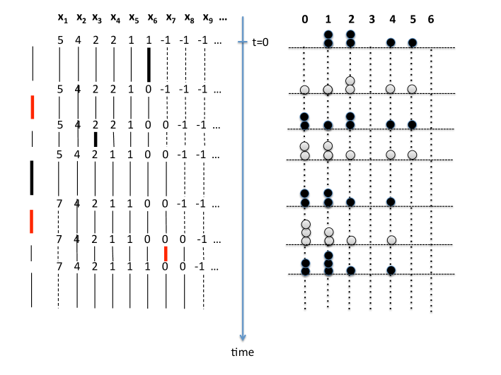
Figure 1: Graphical construction of the flow $T_{t}$ (left panel) and of the process with generator (1.1) (right panel) for a system of size ${\epsilon}^{-1}=6$. The legend for the left panel is as follows: continuous vertical line denotes the clocks of the particles involved in the dynamics; the clock of the boundaries is that on the left; the clock that rings first is depicted with a bold line with color red if it has associated a jump $+1$ and color black if corresponds to a jump $-1$. After jumps particles are re-ordered (if needed). On the right panel the motion in the physical space $[0,6]$ is displayed.

6 Mass transport inequalities

In this section we introduce a partial order among measures based on moving mass to the right, we are evidently in the context of mass transport theory from where we are borrowing the notions used in this section. We work first in the space of particle configurations $\xi$ regarding $\xi$ as a distribution of masses and then in the space $\mathcal{U}$, considering $u\in\mathcal{U}$ as a mass density (which may have a Dirac delta at 0), the notions are the same except for a change of language.

The main goal is to prove inequalities between $\xi_{t}$ and the auxiliary processes $\xi_{t}^{(\delta,\pm)}$ (recall that the hydrodynamic limit of the latter is known since Section 4) and then derive analogous inequalities for $S_{t}^{(\delta,\pm)}(u)$ and their limit as $\delta\to 0$.

We tacitly suppose in the sequel that the configurations $\xi$ are in $\mathcal{X}$ as specified in the beginning of Section 5.

Definition 6.1 (Partial order).

For any $\xi,\xi^{\prime}\in\mathcal{X}$, we say that $\xi\leq\xi^{\prime}$ iff

$$F_{\epsilon}(x;\xi)\leq F_{\epsilon}(x;\xi^{\prime})\quad\text{for all $x\in[0,{\epsilon}^{-1}+1]$}\;.$$ (6.1)

Observe that $\xi\leq\xi^{\prime}$ has not the usual meaning, i.e. $\xi(x)\leq\xi^{\prime}(x)$ for all $x$ !  The notion of order has rather to be interpreted in the sense of “the interfaces” $F_{\epsilon}(x;\xi)=\sum_{y\geq x}\xi(y)$, see Definition 2.3 and Figure 2 for a visual illustration. One can easily check that the above “$\leq$” relation has indeed all the properties of a partial order. Same considerations apply to the case of continuous mass distributions as in (2.12) where the notion is well known and much used in mass transport theory.

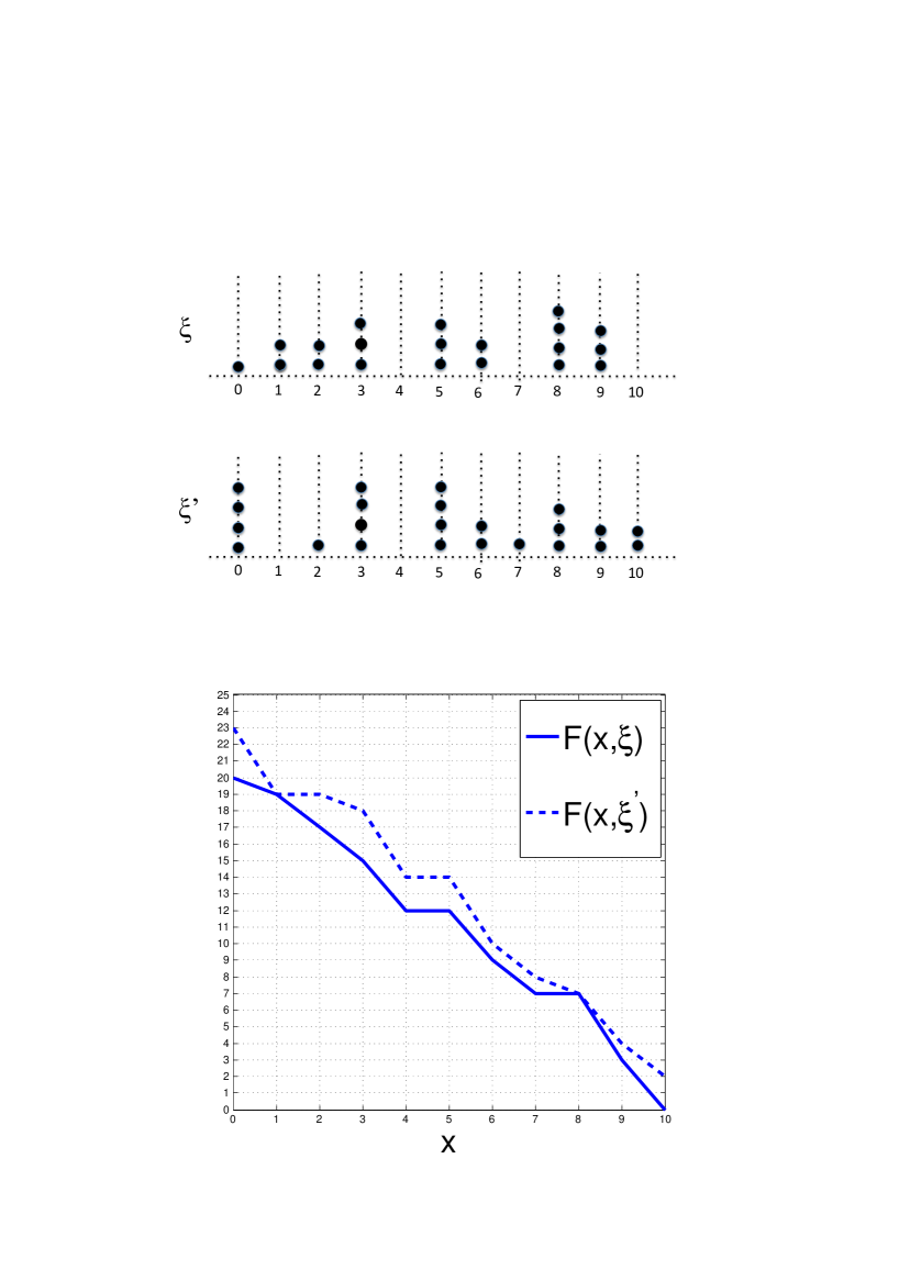
Figure 2: An example of two particle configurations $(\xi,\xi^{\prime})$ related by the inequality $\xi\leq\xi^{\prime}$ for ${\epsilon}^{-1}=10$. Note that for the sites $x\in\{1,2,8,9\}$ one has $\xi(x)>\xi^{\prime}(x)$. However the interface of $\xi$ is below the interface of $\xi^{\prime}$ for all $x\in[0,10]$.

The equivalence with the previous statement about moving mass to the right is established next. We first introduce a partial order in $\mathcal{X}^{\rm ord}$ by saying that $\underline{x}\leq\underline{x}^{\prime}$ iff $x_{i}\leq x^{\prime}_{i}$ for all $i$. Since there is a one-to-one correspondence between $\mathcal{X}$ (see Definition 6.1) and $\mathcal{X}^{\rm ord}$ this defines a priori a new order in $\mathcal{X}$, but the two orders are the same as proved in the following Proposition.

Proposition 6.1.

The conditions: (1)  $\xi\leq\xi^{\prime}$; (2)  $\underline{x}_{\xi}\leq\underline{x}_{\xi^{\prime}}$ (see Definition 5.1) are equivalent. Moreover, let $\underline{x}=(x_{1},..,x_{m})$ and $\underline{x}^{\prime}=(x^{\prime}_{1},..,x^{\prime}_{n})$ be sequences with values in $[0,{\epsilon}^{-1}+1]$ then $\xi_{\underline{x}}\leq\xi_{\underline{x}^{\prime}}$ (see (5.1)) iff $n\geq m$ and there is a one to one map $i_{j}$ from $\{1,..,m\}$ into $\{1,..,n\}$ so that $x^{\prime}_{i_{j}}\geq x_{j}$ for all $j=1,..,m$.

Proof. Equivalence of (1) and (2). Shorthand $\underline{x}=\underline{x}_{\xi}$, $\underline{x}^{\prime}=\underline{x}_{\xi^{\prime}}$.

Suppose (2) holds, then

$$F_{\epsilon}(x;\xi)=\sum_{i\geq 1}\mathbf{1}_{x_{i}\geq x}\leq\sum_{i\geq 1}\mathbf{1}_{x^{\prime}_{i}\geq x}=F_{\epsilon}(x;\xi^{\prime})\quad\text{for all $x\geq 0$}$$ (6.2)

hence $(2)\Rightarrow(1)$.

Suppose (1) holds and let $\underline{x}=(x_{1},..,x_{m})$ and $\underline{x}^{\prime}=(x^{\prime}_{1},..,x^{\prime}_{n})$. Then $n\geq m$ because otherwise $F_{\epsilon}(0;\xi)>F_{\epsilon}(0;\xi^{\prime})$. We also have that $x_{i}\leq x^{\prime}_{i}$ for $i\leq m$: suppose by contradiction that $x_{k}>x^{\prime}_{k}$ then $F_{\epsilon}(x_{k};\xi)\geq k$ while $F_{\epsilon}(x_{k};\xi^{\prime})<k$, hence the contradiction. Thus $(1)\Rightarrow(2)$.

Let $\underline{x}=(x_{1},..,x_{m})$ and $\underline{x}^{\prime}=(x^{\prime}_{1},..,x^{\prime}_{n})$ be sequences with values in $[0,{\epsilon}^{-1}+1]$ such that $n\geq m$ and with a one to one map $i_{j}$ as in the text of the proposition. Then

$$F_{\epsilon}(x;\xi_{\underline{x}})=\sum_{j\geq 1}^{m}\mathbf{1}_{x_{j}\geq x}\leq\sum_{j\geq 1}^{m}\mathbf{1}_{x^{\prime}_{i_{j}}\geq x}\leq F_{\epsilon}(x;\xi_{\underline{x}^{\prime}})$$ (6.3)

hence $\xi_{\underline{x}}\leq\xi_{\underline{x}^{\prime}}$. To prove the converse statement we suppose that $\underline{x}=(x_{1},..,x_{m})$ and $\underline{x}^{\prime}=(x^{\prime}_{1},..,x^{\prime}_{n})$ are such that $\xi:=\xi_{\underline{x}}\leq\xi^{\prime}:=\xi_{\underline{x}^{\prime}}$. Then $\underline{y}:=\underline{x}_{\xi}\leq\underline{y}^{\prime}=\underline{x}_{\xi^{\prime}}$, and there are one to one maps $\ell_{j}:\{1,..,m\}$ onto itself and $\ell^{\prime}_{j}:\{1,..,n\}$ onto itself so that $y_{\ell_{j}}=x_{j}$ and $x^{\prime}_{\ell^{\prime}_{h}}=y^{\prime}_{h}$. Then $x_{j}\leq x^{\prime}_{i_{j}}$ with $i_{j}=\ell^{\prime}_{\ell_{j}}$.

∎

As a corollary we have

Lemma 6.2.

If $\underline{x}\leq\underline{x}^{\prime}$ then

$$a^{\pm}_{i}\underline{x}\leq a^{\pm}_{i}\underline{x}^{\prime},\;\;i\geq 0;\qquad\underline{x}\leq a^{\pm}_{0}\underline{x}^{\prime}$$

(6.4)

$$a^{+}_{0}\underline{x}\leq\underline{x}^{\prime}\;\;\text{if }\;N(\underline{x})<N(\underline{x}^{\prime})\qquad a^{-}_{0}\underline{x}\leq\underline{x}^{\prime}\;\;\text{if }\;M(\underline{x})<M(\underline{x}^{\prime})$$

Proof. The inequality $\underline{x}\leq a^{\pm}_{0}\underline{x}^{\prime}$ holds trivially because $a^{\pm}_{0}\underline{x}^{\prime}$ does not decrease the entries of $\underline{x}^{\prime}$. Let us next consider the other inequalities involving $a^{+}_{0}$. Let $k=N(\underline{x})+1$, then $\underline{y}:=a^{+}_{0}\underline{x}$ has $y_{k}=0$, while $x_{k}=-1$ (all the other entries are unchanged). If $N(\underline{x}^{\prime})>N(\underline{x})$ then $x^{\prime}_{k}\geq 0$ and the last inequality in (6.2) is satisfied. If $N(\underline{x}^{\prime})=N(\underline{x})$ then $x^{\prime}_{k}=-1$ but $y^{\prime}_{k}=0$, where $\underline{y}^{\prime}=a^{+}_{0}\underline{x}^{\prime}$, hence the first equality in (6.2).

Let us next consider $a^{-}_{0}$. If $M(\underline{x})=N(\underline{x})$ then $a^{-}_{0}\underline{x}=\underline{x}$ and therefore is $\leq\underline{x}^{\prime}\leq a_{0}^{-}\underline{x}^{\prime}$. Let then $m=M(\underline{x})+1\leq N(\underline{x})$. Then $\underline{y}:=a^{-}_{0}\underline{x}$ has $y_{m}={\epsilon}^{-1}+1$. If $M(\underline{x}^{\prime})>M(\underline{x})$, then $x^{\prime}_{m}={\epsilon}^{-1}+1$. If instead $M(\underline{x}^{\prime})=M(\underline{x})$ then $x_{m}\leq x^{\prime}_{m}$ hence $x^{\prime}_{m}\in[0,{\epsilon}^{-1}]$ and $\underline{y}^{\prime}=a^{-}_{0}\underline{x}^{\prime}$ has $y^{\prime}_{m}={\epsilon}^{-1}+1$.

Let next $\underline{y}=a^{\pm}_{i}\underline{x}$ and $\underline{y}^{\prime}=a^{\pm}_{i}\underline{x}^{\prime}$ with $i\geq 1$ and for the sake of definiteness let us just consider the $+$ case. $\underline{y}=\underline{x}$ if $i\leq M(\underline{x})$ and $i>N(\underline{x})$. In the former case $x^{\prime}_{i}={\epsilon}^{-1}+1$ is also unchanged, in the latter $x_{i}=-1$ and again the inequality holds trivially. Let us then suppose that $M(\underline{x})<i\leq N(\underline{x})$ and suppose that this holds as well for $\underline{x}^{\prime}$ (otherwise $x^{\prime}_{i}={\epsilon}^{-1}+1$). Then $\min\{x_{i}+1,{\epsilon}^{-1}\}\leq\min\{x^{\prime}_{i}+1,{\epsilon}^{-1}\}$ hence the desired inequality applying the last statement in Proposition 6.1. ∎

As already mentioned we ultimately need inequalities for the restrictions $\underline{x}\cap[0,{\epsilon}^{-1}]$ of the configurations to the physical space. We shall use the following simple observation:

Lemma 6.3.

If $\underline{x}\leq\underline{x}^{\prime}$ then $N(\underline{x})\leq N(\underline{x}^{\prime})$ and $M(\underline{x})\leq M(\underline{x}^{\prime})$, however $(\underline{x}\cap[0,{\epsilon}^{-1}])\leq(\underline{x}^{\prime}\cap[0,{\epsilon}^{-1}])$ requires that $M(\underline{x})=M(\underline{x}^{\prime})$. In particular if $\underline{x}\leq\underline{x}^{\prime}$:

$$(\underline{x}\cap[0,{\epsilon}^{-1}])\leq(\underline{x}^{\prime}\cap[0,{\epsilon}^{-1}])\;\;{\rm if}\;\;N(\underline{x})=N(\underline{x}^{\prime}),\,\;\;M(\underline{x})=M(\underline{x}^{\prime})$$ (6.5)

Definition 6.2 (Stochastic order).

A process $(\xi_{t})_{t\geq 0}$ is stochastically smaller than a process $(\xi^{\prime}_{t})_{t\geq 0}$, writing in short $\xi_{t}\leq\xi^{\prime}_{t}$ (stochastically), if they can be both realized on a same space where the inequality holds pointwise almost surely.

We shall prove stochastic order by realizing the processes on the same space $({\Omega},P)$ of Definition 5.2.

Definition 6.3.

A map $f:\mathcal{X}^{\rm ord}\to\mathcal{X}^{\rm ord}$ preserves order if $\underline{x}\leq\underline{x}^{\prime}$ implies $f(\underline{x})\leq f(\underline{x}^{\prime})$.

The first inequality in (6.2) proves that all the maps $a_{i}^{\pm}$ preserve order and since all the flows have been defined in terms of products of such maps:

Theorem 6.4 (Stochastic inequalities).

All the maps $T^{(\delta,\pm)}_{m{\epsilon}^{-2}\delta}(\cdot,{\omega})$, $T^{0}_{t}(\cdot,{\omega})$ and $T_{t}(\cdot,{\omega})$, preserve order.

To compare the flows $T^{(\delta,\pm)}_{t}$ and $T_{t}$ we shall use the following lemma:

Lemma 6.5.

Let $i\geq 1$, then

$$a_{0}^{{\sigma}_{0}}a_{i}^{{\sigma}_{i}}\underline{x}\leq a_{i}^{{\sigma}_{i}}a_{0}^{{\sigma}_{0}}\underline{x}$$ (6.6)

Proof. Let ${\sigma}_{0}=+$. Call $\underline{y}=a_{0}^{+}\underline{x}$, then by the second inequality in (6.2), $\underline{x}\leq\underline{y}$. Since $a_{i}^{{\sigma}_{i}}$ preserves order: $a_{i}^{{\sigma}_{i}}\underline{x}\leq a_{i}^{{\sigma}_{i}}\underline{y}$ and since $N(\underline{y})=N(\underline{x})+1$ we have (6.6) (having used the third inequality in (6.2)). Let ${\sigma}_{0}=-$. Call $\underline{y}=a_{0}^{-}\underline{x}$, then by the second inequality in (6.2), $\underline{x}\leq\underline{y}$. Since $a_{i}^{{\sigma}_{i}}$ preserves order: $a_{i}^{{\sigma}_{i}}\underline{x}\leq a_{i}^{{\sigma}_{i}}\underline{y}$ and since $M(\underline{y})=M(\underline{x})+1$ we have again (6.6) (having used the fourth inequality in (6.2)). ∎

Corollary 6.6.

Let $\{(i_{j},{\sigma}_{j})\}$ a sequence of $n>1$ pairs with $i_{j}\geq 0$, ${\sigma}_{j}\in\{+,-\}$. An exchange at $(h,h+1)$, $h+1\leq n$, is the new sequence $\{(i^{\prime}_{j},{\sigma}^{\prime}_{j})\}$ where $(i^{\prime}_{j},{\sigma}^{\prime}_{j})=(i_{j},{\sigma}_{j})$ for $j\neq h,h+1$ and $(i^{\prime}_{h},{\sigma}^{\prime}_{h})=(i_{h+1},{\sigma}_{h+1})$, $(i^{\prime}_{h+1},{\sigma}^{\prime}_{h+1})=(i_{h},{\sigma}_{h})$. We then say that an exchange at $(h,h+1)$ is “allowed” if $i_{h}=0$ and $i_{h+1}>0$.

Then if $\pi$ is a permutation obtained by applying repeatedly allowed exchanges starting from $\{(i_{j},{\sigma}_{j})\}$ so that the final sequence is $\{(i_{\pi(j)},{\sigma}_{\pi(j)})\}$

$$\prod_{j=1}^{n}a_{i_{j}}^{{\sigma}_{j}}\underline{x}\leq\prod_{j=1}^{n}a_{i_{\pi(j)}}^{{\sigma}_{\pi(j)}}\underline{x}$$ (6.7)

Call $\{(a_{j},{\sigma}_{j})\}$ the sequence associated to $T^{(\delta,-)}_{m{\epsilon}^{-2}\delta}(\underline{x},{\omega})$ and $\{(a^{\prime}_{j},{\sigma}^{\prime}_{j})\}$ the one associated to $T_{m{\epsilon}^{-2}\delta}^{(\delta^{\prime},-)}(\underline{x},{\omega})$, $\delta=k\delta^{\prime}$: then the latter is obtained by repeated allowed exchanges from the former, hence

$$T_{m{\epsilon}^{-2}\delta}^{(\delta,-)}(\underline{x},{\omega})\leq T_{m{\epsilon}^{-2}\delta}^{(\delta^{\prime},-)}(\underline{x},{\omega})$$

Also the sequence $\{(a^{\prime\prime}_{j},{\sigma}^{\prime\prime}_{j})\}$ associated to $T_{m{\epsilon}^{-2}\delta}(\underline{x},{\omega})$ is obtained by repeated allowed exchanges from $\{(a^{\prime}_{j},{\sigma}^{\prime}_{j})\}$, hence

$$T_{m{\epsilon}^{-2}\delta}^{(\delta^{\prime},-)}(\underline{x},{\omega})\leq T_{m{\epsilon}^{-2}\delta}(\underline{x},{\omega})$$

The sequence $\{(a^{\prime\prime\prime}_{j},{\sigma}^{\prime\prime\prime}_{j})\}$ associated to $T_{m{\epsilon}^{-2}\delta}^{(\delta^{\prime},+)}(\underline{x},{\omega})$ is obtained by repeated allowed exchanges from $\{(a^{\prime\prime}_{j},{\sigma}^{\prime\prime}_{j})\}$, hence

$$T_{m{\epsilon}^{-2}\delta}\leq T_{m{\epsilon}^{-2}\delta}^{(\delta^{\prime},+)}(\underline{x},{\omega})$$

Finally the sequence $\{(a^{*}_{j},{\sigma}^{*}_{j})\}$ associated to $T_{m{\epsilon}^{-2}\delta}^{(\delta,+)}(\underline{x},{\omega})$ is obtained by repeated allowed exchanges from $\{(a^{\prime\prime\prime}_{j},{\sigma}^{\prime\prime\prime}_{j})\}$, hence

$$T_{m{\epsilon}^{-2}\delta}^{(\delta^{\prime},+)}(\underline{x},{\omega})\leq T_{m{\epsilon}^{-2}\delta}^{(\delta,+)}(\underline{x},{\omega})$$

We have thus proved:

Theorem 6.7 (Stochastic inequalities).

Denoting by $\xi_{m{\epsilon}^{-2}\delta}^{(\delta,\pm)}$ and $\xi_{t}^{(\delta,\pm)}$ the configurations $\xi_{T_{m{\epsilon}^{-2}\delta}^{(\delta,-)}(\underline{x},{\omega})}$ and $\xi_{T_{t}(\underline{x},{\omega})}$ restricted to $x\in[0,{\epsilon}^{-1}]$ we have for any $\delta=k\delta^{\prime}$, $k$ a positive integer,

$$\xi_{m{\epsilon}^{-2}\delta}^{(\delta,-)}\leq\xi_{m{\epsilon}^{-2}\delta}^{(\delta^{\prime},-)}\leq\xi_{m{\epsilon}^{-2}\delta}\leq\xi_{m{\epsilon}^{-2}\delta}^{(\delta^{\prime},+)}\leq\xi_{m{\epsilon}^{-2}\delta}^{(\delta,+)}$$ (6.8)

Proof. We have already proved the inequality for the configurations on $[-1,{\epsilon}^{-1}+1]$, thus the proof of (6.8) follows from (6.5) and (5.9). ∎

The theorem has its continuum analogue which can be proved directly, see Section 4 of [3], but it can also be deduced from Theorem 6.7, as we shall see.

Theorem 6.8 (Macroscopic inequalities).

Let $u\in L^{\infty}([0,1],\mathbb{R}_{+})$, $F(0;u)>0$. Let $\delta:j\delta<F(0;u)$ and $\delta^{\prime}$ such that $\delta=k\delta^{\prime}$ with $k$ a positive integer. Then

$$S_{m\delta}^{(\delta,-)}(u)\leq S_{m\delta}^{(\delta^{\prime},-)}\leq S_{m\delta}^{(\delta^{\prime},+)}\leq S_{m\delta}^{(\delta,+)}$$ (6.9)

Moreover the maps $K^{(\delta)}$, ${G^{\rm neum}_{t}}*$ and $S_{t}^{(\delta,\pm)}$ on $\mathcal{U}_{\delta}$, see (2.14), preserve order.

Proof. (6.9) follows from (6.8) and (4.2). Proof that $K^{(\delta)}u\leq K^{(\delta)}v$, $u,v\in\mathcal{U}_{\delta}$. We have

$$K^{(\delta)}u-K^{(\delta)}v=(c_{u}-c_{v})D_{0}+(\rho_{u}-\rho_{v})\mathbf{1}_{r\leq R_{\delta}(u)}-\rho_{v}\mathbf{1}_{R_{\delta}(u)<r\leq R_{\delta}(v)}$$

where $R_{\delta}(w):F(R_{\delta}(w);w)=j\delta$. Hence

$$F(r;K^{(\delta)}u)-F(r;K^{(\delta)}v)=\Big{(}F(r;u)-F(r;v)\Big{)}\mathbf{1}_{r\leq R_{\delta}(u)}-\mathbf{1}_{r>R_{\delta}(u)}\int_{r}^{R_{\delta}(v)}\rho_{v}(r^{\prime})$$

which is therefore $\leq 0$.

The property that ${G^{\rm neum}_{t}}*$ preserves the order is inherited from the same property for the independent flow $T^{0}_{t}$. As a consequence of the two previous statements we have that also $S^{(\delta,\pm)}_{t}$ preserves the order (see the definition in (2.14)). ∎

7 Regularity properties of the barriers

In this section we shall prove some regularity properties of the barriers $S_{t}^{(\delta,\pm)}(u)$, $u\in L^{\infty}([0,1],\mathbb{R}_{+})$, $F(0;u)>j\delta$ (the barriers are defined in Definition 2.5).

By the smoothness of $G_{t}^{\rm neum}(r,r^{\prime})$, $t>0$, it is easy to prove that for any $n>0$, $S^{(\delta,+)}_{n\delta}(u)$ is in $C^{\infty}$ while $S^{(\delta,-)}_{n\delta}(u)$ is equal to $j\delta D_{0}$ plus a function which is $C^{\infty}$ in the interior of its support. Such a smoothness however, being inherited from $G^{\rm neum}_{\delta}$, depends on $\delta$, while we want properties which hold uniformly as $\delta\to 0$.

The properties of the Green functions that we use in this section are:

$$G_{t}^{\rm neum}(r,r^{\prime})=G_{t}^{\rm neum}(r^{\prime},r)\leq\frac{c(1+\sqrt{t})}{\sqrt{t}},\quad|\frac{d}{dr}G_{t}^{\rm neum}(r,r^{\prime})|\leq\frac{c}{t}$$ (7.1)

$$\int dr^{\prime}G^{\rm neum}_{t}(r,r^{\prime})=1$$ (7.2)

$$\int_{|r^{\prime}-r|>X}dr^{\prime}G^{\rm neum}_{t}(r,r^{\prime})\leq\sqrt{2}e^{-X^{2}/(4t)},\qquad\forall X>0$$ (7.3)

(7.3) is proved by writing

$$\int_{|r^{\prime}-r|>X}dr^{\prime}G^{\rm neum}_{t}(r,r^{\prime})\leq\int_{|r^{\prime}-r|>X}dr^{\prime}G_{t}(r,r^{\prime}),\quad G_{t}(r,r^{\prime})=\frac{e^{-(r-r^{\prime})^{2}/(2t)}}{\sqrt{2\pi t}}$$

and then bounding

$$\int_{|r^{\prime}-r|>X}dr^{\prime}G_{t}(r,r^{\prime})\leq e^{-X^{2}/(4t)}\sqrt{2}\int dr\frac{e^{-r^{2}/(4t)}}{\sqrt{4\pi t}}$$

Such bounds are verified also by the Green function for the Neumann problem in $[0,\ell]$ for any $\ell>0$ and $\ell=\infty$ as well, so that the analysis in this section extends to all such cases. Observe that if $\ell$ is finite and positive the bound on the derivative is much better:

$$\Big{|}\frac{d}{dr}G_{t}^{\rm neum}(r,0)\Big{|}\leq\frac{ce^{-bt}}{t},\quad b>0,c>0$$

but we shall only use (7.1), (7.2) and (7.3) to have what follows valid also in the spatial domain $[0,\infty)$.

The main results in this section are:

Theorem 7.1 (Space and time equicontinuity).

Let $u\in L^{\infty}([0,1],\mathbb{R}_{+})$, $F(0;u)>0$. Then

• $F(0;S_{t}^{(\delta,\pm)}(u))=F(0;u)$ for all $\delta>0$ such that $F(0;u)>j\delta$ and all $t=n\delta$, $n\in\mathbb{N}$.

• There is a constant $c$ so that for any $\delta>0$: $F(0;u)>j\delta$

  $$\|S^{(\delta,+)}_{t}(u)\|_{\infty}\leq c\left\{\begin{array}[]{ll}j+\|u\|_{\infty}&\text{for all $t\in\delta{\mathbb{N}},\>t\leq 1$}\\ j+F(0;u)&\text{for all $t\in\delta{\mathbb{N}},\>t>1$}\end{array}\right.$$ (7.4)

  Same bounds hold for $\{S^{(\delta,-)}_{t}(u)-jD_{0}\}$.

• Given any time ${\sigma}>0$ the following holds. For any $\zeta>0$ there are $\tau_{\zeta}>0$ and $d_{\zeta}>0$ so that for any $\delta\in(0,{\sigma})$: $F(0;u)>j\delta$, for any $t\geq{\sigma}$ in $\delta\mathbb{N}$, for any $t^{\prime}\in\delta\mathbb{N}$, $t^{\prime}\in(t,t+\tau_{\zeta})$ and for any $r$ and $r^{\prime}$ such that $|r-r^{\prime}|<d_{\zeta}$,

  $$|S^{(\delta,+)}_{t}(u)(r)-S^{(\delta,+)}_{t}(u)(r^{\prime})|<\zeta,\quad|S^{(\delta,+)}_{t^{\prime}}(u)(r)-S^{(\delta,+)}_{t}(u)(r)|<\zeta$$ (7.5)

• For all $\delta>0$ such that $F(0;u)>j\delta$ and all $t>0$ in $\delta\mathbb{N}$

  $$F\Big{(}0;|S_{t}^{(\delta,+)}(u)-S_{t}^{(\delta,-)}(u)|\Big{)}\leq 4j\delta$$ (7.6)

Proof.

$\bullet$  $F(0;S_{t}^{(\delta,\pm)}(u))=F(0;u)$ because by (7.2) $G_{\delta}^{\rm neum}$ preserves the mass, as well as $K^{(\delta)}$, by its very definition, see (2.15)).

$\bullet$  Proof of (7.4). Let $t=n\delta$, $n$ a positive integer, then

$$S^{(\delta,+)}_{t}(u)(r)\leq\int dr^{\prime}G_{\delta}^{\rm neum}(r,r^{\prime})S^{(\delta,+)}_{t-\delta}(u)(r^{\prime})+j\delta G_{\delta}^{\rm neum}(r,0)$$

The inequality is because we are not taking into account the “loss part” in the action of $K^{(\delta)}$. Iterating we get for $s=m\delta$, $m<n$ a non negative integer,

$$S^{(\delta,+)}_{t}(u)(r)\leq\int dr^{\prime}G_{t-s}^{\rm neum}(r,r^{\prime})S^{(\delta,+)}_{s}(u)(r^{\prime})+j\delta\sum_{k=1}^{n-m}G_{k\delta}^{\rm neum}(r,0)$$ (7.7)

Let $n_{\delta}$ be the smallest integer such that $\delta n_{\delta}\geq 1$ and suppose that in (7.7) $t<\delta n_{\delta}$ and $s=0$. By (7.2) the integral in (7.7) is bounded by $\|u\|_{\infty}$ whereas by (7.1) the sum is bounded by $c^{\prime\prime}j\sqrt{n\delta}\leq c^{\prime\prime}j$. Thus (7.4) is proved for $t\leq 1$.

Let us next take $t=\delta n_{\delta}$ and $s=0$ in (7.7). Then using (7.1) we bound the integral in (7.7) by $c^{\prime}F(0;u)(\delta n_{\delta})^{-1/2}\leq c^{\prime}F(0;u)$. As before the last term in (7.7) is bounded by $c^{\prime\prime}j\sqrt{\delta n_{\delta}}\leq 2c^{\prime\prime}j$ so that (we may suppose $c^{\prime}<2c^{\prime\prime}$)

$$\|S^{(\delta,+)}_{n_{\delta}\delta}(u)\|_{\infty}\leq 2c^{\prime\prime}(F(0;u)+j)$$

By the same argument for any integer $k\geq 1$

$$\|S^{(\delta,+)}_{kn_{\delta}\delta}(u)\|_{\infty}\leq 2c^{\prime\prime}\{F\Big{(}0;S^{(\delta,+)}_{(k-1)\delta n_{\delta}}(u)\Big{)}+j\}=2c^{\prime\prime}(F(0;u)+j)$$ (7.8)

the last equality because we have already proved that mass is conserved. Thus (7.4) is proved for $t\in(\delta n_{\delta})\mathbb{N}$. Let now $m=kn_{\delta}$ and $kn_{\delta}<n\leq(k+1)n_{\delta}$ $k$ a positive integer. The last term in (7.7) is bounded again by $2c^{\prime\prime}j$, whereas the integral is smaller than $\|S^{(\delta,+)}_{kn_{\delta}\delta}(u)\|_{\infty}$. Thus (7.4) follows from (7.8) when $t\geq 1$.

We next prove the analogue of (7.4) for

$$\rho^{(\delta,-)}_{t}:=S^{(\delta,-)}_{t}(u)-j\delta D_{0},\qquad t>0\in\delta\mathbb{N}$$ (7.9)

Let $t=n\delta$, $s=m\delta$, $n>m$ in $\mathbb{N}$, just as before. Recalling the definition (7.9), we have

$$\rho^{(\delta,-)}_{n\delta}=K^{(\delta)}[G^{\rm neum}_{\delta}*S^{(\delta,-)}_{(n-1)\delta}(\rho_{0})]-j\delta D_{0}=\mathbf{1}_{[0,R]}\,\,\,G^{\rm neum}_{\delta}*\big{[}\rho^{(\delta,-)}_{(n-1)\delta}+j\delta D_{0}\big{]}$$

where $\mathbf{1}_{[0,R]}$ is the characteristic function of the set $[0,R]$ and $R$ is such that

$$\int_{R}^{1}G^{\rm neum}_{\delta}*\big{[}\rho^{(\delta,-)}_{(n-1)\delta}+j\delta D_{0}\big{]}(r)=j\delta$$

Then

$$\hskip-28.45274pt\rho^{(\delta,-)}_{n\delta}(r)=\mathbf{1}_{r\leq R}\Big{(}j\delta G_{\delta}^{\rm neum}(r,0)+G^{\rm neum}_{\delta}*\rho^{(\delta,-)}_{(n-1)\delta}(r)\Big{)}$$

$$\leq j\delta G_{\delta}^{\rm neum}(r,0)+G^{\rm neum}_{\delta}*\rho^{(\delta,-)}_{(n-1)\delta}(r)$$ (7.10)

After iterating (7.10) we get

$$\rho^{(\delta,-)}_{t}(r)\leq j\delta\sum_{k=1}^{n-m}G_{k\delta}^{\rm neum}(r,0)+\int dr^{\prime}G_{t-s}^{\rm neum}(r,r^{\prime})\rho^{(\delta,-)}_{s}(r^{\prime})$$ (7.11)

which has the same structure as (7.7). The analysis after (7.7) extends to the present case and yields the proof of (7.4) for $\rho^{(\delta,-)}_{t}$.

The proof of (7.5) and (7.6) will be given after the following lemma.

Lemma 7.2.

There is a constant $c$ so that the following holds. For all $\delta>0$ such that $F(0;u)>j\delta$ and for all $0\leq s<t$, $s,t\in\delta\mathbb{N}$, $t-s\leq 1$, we write

$$w_{s,t}^{(\delta,+)}(r):=\int dr^{\prime}G_{t-s}^{\rm neum}(r,r^{\prime})S^{(\delta,+)}_{s}(u)(r^{\prime}),\;\;\;v_{s,t}^{(\delta,+)}:=S^{(\delta,+)}_{t}(u)-w_{s,t}^{(\delta,+)}$$ (7.12)

Then

$$\sup_{r,r^{\prime}\in[0,1]}|w_{s,t}^{(\delta,+)}(r)-w_{s,t}^{(\delta,+)}(r^{\prime})|\leq c\|u\|_{\infty}\frac{|r-r^{\prime}|}{t-s}$$ (7.13)

$$F(0;|v_{s,t}^{(\delta,+)}|)\leq 2j(t-s),\quad\|v_{s,t}^{(\delta,+)}\|_{\infty}\leq cj\sqrt{t-s}$$ (7.14)

Proof. By (7.4) and the second inequality in (7.1) we get

$$|w_{s,t}^{(\delta,+)}(r)-w_{s,t}^{(\delta,+)}(r^{\prime})|\leq\|S^{(\delta,+)}_{s}(u)\|_{\infty}\int|G^{\rm neum}_{t-s}(r,z)-G^{\rm neum}_{t-s}(r^{\prime},z)|\,dz\leq c\frac{|r^{\prime}-r^{\prime\prime}|}{t-s}\,\|u\|_{\infty}$$

which proves (7.13).

We already have an upper bound for $S^{(\delta,+)}_{t}(u)(r)$ as given by (7.7) and want to find a lower bound. We first define for any $\tau\in\delta\mathbb{N}$

$$v^{(\delta)}_{\tau}(r)=\mathbf{1}_{r\geq R}S^{(\delta,+)}_{\tau}(u)(r),\quad R:\;\;\int v^{(\delta)}_{\tau}(r)=j\delta$$ (7.15)

By (7.4)

$$\|v^{(\delta)}_{\tau}\|_{\infty}\leq C,\quad C=c\Big{(}j+\|u\|_{\infty}\Big{)}$$ (7.16)

By neglecting the contribution of $jD_{0}$ we get:

$$S^{(\delta,+)}_{t}(u)\geq G^{\rm neum}_{\delta}*\Big{(}S^{(\delta,+)}_{t-\delta}(u)-v^{(\delta)}_{t-\delta}\Big{)}$$

and by iteration:

$$S^{(\delta,+)}_{t}(u)\geq G^{\rm neum}_{t-s}*S^{(\delta,+)}_{s}(u)-\sum_{k=m}^{n-1}G^{\rm neum}_{(n-k)\delta}*v^{(\delta)}_{k\delta}$$

Combining the upper and the lower bound and recalling (7.12)

$$|v_{s,t}^{(\delta,+)}|\equiv|S^{(\delta,+)}_{t}(u)-G^{\rm neum}_{t-s}*S^{(\delta,+)}_{s}(u)|\leq\sum_{k=m}^{n-1}G^{\rm neum}_{(n-k))\delta}*v^{(\delta)}_{k\delta}+j\delta\sum_{k=1}^{n-m}G_{k\delta}^{\rm neum}(r,0)$$ (7.17)

By (7.15) and (7.1)

$$\|\sum_{k=m+1}^{n}G^{\rm neum}_{(n-k)\delta}*v^{(\delta)}_{k\delta}\|_{\infty}\leq cj\sqrt{\delta}\sqrt{n-m}=cj\sqrt{t-s}$$

and by (7.1)

$$\|j\delta\sum_{k=1}^{n-m}G_{k\delta}^{\rm neum}(r,0)\|_{\infty}\leq cj\sqrt{\delta}\sqrt{n-m}=cj\sqrt{t-s}$$

so that $\|v_{s,t}^{(\delta,+)}\|_{\infty}\leq cj\sqrt{t-s}$ and the second inequality in (7.14) is proved. To prove the first one we use (7.17), (7.12) and (7.2) to write

$$F(0;|v^{(\delta,+)}_{s,t}|)\leq j\delta(t-s)+F\Big{(}0;\sum_{k=m}^{n-1}G^{\rm neum}_{(n-k)\delta}*v^{(\delta)}_{k\delta}\Big{)}\leq 2j\delta(t-s)$$

which concludes the proof of (7.14).

∎

We resume the proof of Theorem 7.1 by proving:

$\bullet$   Proof of the first inequality in (7.5) (space equicontinuity). Recalling that $\delta<{\sigma}$ we may suppose (with no loss of generality) that

$$\zeta<2c^{\prime}\sqrt{{\sigma}-\delta},\quad c^{\prime}:=c(j+\|u\|_{\infty})$$ (7.18)

with $c$ the constant in (7.13)–(7.14). Then, given any such $\zeta>0$, we must find $d_{\zeta}>0$ so that

$$\sup_{|r-r^{\prime}|<d_{\zeta}}\;|S^{(\delta,+)}_{t}(u)(r)-S^{(\delta,+)}_{t}(u)(r^{\prime})|<\zeta,\quad t\in\delta\mathbb{N},\;t\geq{\sigma}$$ (7.19)

By (7.13) and (7.14)

$$|S^{(\delta,+)}_{t}(u)(r)-S^{(\delta,+)}_{t}(u)(r^{\prime})|\leq c^{\prime}\frac{|r-r^{\prime}|}{{t-s}}+c^{\prime}\sqrt{t-s}$$ (7.20)

We shall prove (7.19) with

$$d_{\zeta}<\zeta^{3}\min\Big{\{}\frac{1}{4c^{\prime}(2c^{\prime})^{2}}\;;\;\frac{1}{c^{\prime\prime}(2c^{\prime})^{2}}\Big{\}}$$ (7.21)

where $c^{\prime\prime}$ is a constant which will be specified later.

We first consider the case when $(2c^{\prime})^{2}\delta<\zeta^{2}$. We then choose $s<t$ as the smallest time in $\delta\mathbb{N}$ such that $2c^{\prime}\sqrt{t-s}<\zeta$. Since $t-s=k\delta$, for $s$ to exist it must be that $(2c^{\prime})^{2}\delta<\zeta^{2}$ which is indeed the case presently considered. On the other hand by (7.18), $s\geq\delta$. Then, by the minimality of $s$, $2c^{\prime}\sqrt{t-s+\delta}\geq\zeta$ so that

$$2(t-s)\geq t-s+\delta\geq\frac{\zeta^{2}}{(2c^{\prime})^{2}}$$

By choosing $d_{\zeta}$ as in (7.21) the first term on the right hand side of (7.20) is bounded by

$$c^{\prime}\frac{2(2c^{\prime})^{2}}{\zeta^{2}}d_{\zeta}<\frac{\zeta}{2}$$

hence $|S^{(\delta,+)}_{t}(u)(r)-S^{(\delta,+)}_{t}(u)(r^{\prime})|<\zeta$.

It remains to consider the case when $(2c^{\prime})^{2}\delta\geq\zeta^{2}$. Observe that

$$S^{(\delta,+)}_{t}(u)=G^{\rm neum}_{\delta}*(j\delta D_{0}+v),\quad v=\mathbf{1}_{r\leq R}S^{(\delta,+)}_{t-\delta}(u)$$ (7.22)

where $R$ is such that $\int_{R}^{1}S^{(\delta,+)}_{t-\delta}(u)=j\delta$. Hence by (7.1) the space-derivative of $S^{(\delta,+)}_{t}(u)(r)$ is bounded by

$$\frac{c}{\delta}\Big{(}j\delta+F(0;S^{(\delta,+)}_{t-\delta}(u))\Big{)}=:\frac{c^{\prime\prime}}{\delta}$$

with $c^{\prime\prime}=c(j\delta+F(0;u))$, having used that $F(0;S^{(\delta,+)}_{s}(u))=F(0;u)$.

By (7.21) we then get

$$|S^{(\delta,+)}_{t}(u)(r)-S^{(\delta,+)}_{t}(u)(r^{\prime})|\leq c^{\prime\prime}\delta^{-1}|r-r^{\prime}|\leq c^{\prime\prime}(\frac{\zeta^{2}}{(2c^{\prime})^{2}})^{-1}d_{\zeta}<\zeta$$ (7.23)

$\bullet$   Proof of the second inequality in (7.5) (time equicontinuity). Let $t^{\prime}>t\geq{\sigma}$, $t^{\prime}-t\leq 1$. Then by (7.17) with $t\to t^{\prime}$ and $s\to t$,

$$|S^{(\delta,+)}_{t^{\prime}}(u)-G^{\rm neum}_{t^{\prime}-t}*S^{(\delta,+)}_{t}(u)| \leq \sum_{k=m}^{n-1}G^{\rm neum}_{(n-k))\delta}*v^{(\delta,+)}_{k\delta}+j\delta\sum_{k=1}^{n-m}G_{(n-k)\delta}^{\rm neum}(r,0)$$

$$\leq cj\sqrt{t^{\prime}-t}$$

Hence calling $\zeta^{\prime}=\zeta/4$ and with $C\geq\|S^{(\delta,+)}_{t}(u)\|_{\infty}$ (see (7.4)),

$$|S^{(\delta,+)}_{t^{\prime}}(u)(r)-S^{(\delta,+)}_{t}(u)(r)|\leq\int_{r^{\prime}:|r-r^{\prime}|\geq d_{\zeta^{\prime}}}CG^{\rm neum}_{t^{\prime}-t}(r,r^{\prime})\,dr^{\prime}+\zeta^{\prime}+cj\sqrt{t^{\prime}-t}$$

We choose $\tau_{\zeta}=a\zeta^{8}$, $a$ a positive constant whose value will be specified later. If $\delta>\tau_{\zeta}$ there is no $t^{\prime}:t<t^{\prime}<t+\tau_{\zeta}$ and the second inequality in (7.5) is automatically satisfied. Let then $\delta\leq\tau_{\zeta}$. We choose $a$ so that $cj\sqrt{a\zeta^{4}}<\zeta^{\prime}$. By the decay properties of the Green function, see (7.3),

$$\int_{r^{\prime}:|r-r^{\prime}|\geq d_{\zeta^{\prime}}}G^{\rm neum}_{t^{\prime}-t}(r,r^{\prime})\,dr^{\prime}\leq\sqrt{2}e^{-cd_{\zeta^{\prime}}^{2}/(4\tau_{\zeta})}$$

Since $d_{\zeta}=c\zeta^{3}$ (see the proof of space continuity) for $a$ small enough the above integral is $<\zeta^{\prime}$ as well.

We shall resume the proof of Theorem 7.1 after the following lemma:

Lemma 7.3.

Let $u$ and $v$ be both in $\mathcal{U}_{\delta}$, see (2.14), then

$$F\Big{(}0;|K^{(\delta)}u-K^{(\delta)}v|\Big{)}\leq F\Big{(}0;|u-v|\Big{)},\quad F\Big{(}0;|K^{(\delta)}u-u|\Big{)}\leq 2j\delta$$ (7.24)

Proof. Supposing $R_{\delta}(u)>R_{\delta}(v)$, see (2.15),

$$F\Big{(}0;|K^{(\delta)}u-K^{(\delta)}v|\Big{)} = \int_{0}^{R_{\delta}(v)}|u-v|+\int_{R_{\delta}(v)}^{R_{\delta}(u)}u$$

$$= F\Big{(}0;|u-v|\Big{)}+\int_{R_{\delta}(v)}^{R_{\delta}(u)}(u-|u-v|)-\int_{R_{\delta}(u)}^{\infty}|u-v|$$

We have

$$\int_{R_{\delta}(u)}^{\infty}|u-v|\geq|\int_{R_{\delta}(u)}^{\infty}(u-v)|=j\delta-\int_{R_{\delta}(u)}^{\infty}v=\int_{R_{\delta}(v)}^{R_{\delta}(u)}v$$

so that

$$F\Big{(}0;|K^{(\delta)}u-K^{(\delta)}v|\Big{)}\leq F\Big{(}0;|u-v|\Big{)}-\int_{R_{\delta}(v)}^{R_{\delta}(u)}(v-u+|u-v|)\leq F\Big{(}0;|u-v|\Big{)}$$

The second inequality in (7.24) follows because

$$K^{(\delta)}u-u=j\delta D_{0}-\mathbf{1}_{r>R_{\delta}(u)}u$$

∎

$\bullet$   Proof of (7.6). The proof is actually a corollary of Lemma 7.3 and the maximum principle

$$F\Big{(}0;|G_{t}^{\rm neum}*u-G_{t}^{\rm neum}*v\Big{)}\leq F\Big{(}0;|u-v|\Big{)}$$

Shorthand $G$ for the operator $G_{\delta}^{\rm neum}*$ and

$$\phi:=K^{(\delta)}G\cdots K^{(\delta)}Gu,\qquad\psi:=GK^{(\delta)}\cdots GK^{(\delta)}u$$

so that we need to bound the total variation of $\phi-\psi$. Call

$$v=K^{(\delta)}u,\qquad v_{n}=GK^{(\delta)}\cdots Gv,\qquad u_{n}=GK^{(\delta)}\cdots Gu$$

Thus $u_{n}$ and $v_{n}$ are obtained by applying $G(K^{(\delta)}G)^{n-1}$ to $u$ and respectively $v$. Since $G(K^{(\delta)}G)^{n-1}$ is a contraction we get, using (7.24),

$$F(0;|\psi-\phi|) \leq F(0;|K^{(\delta)}u_{n}-v_{n}|)\leq F(0;|K^{(\delta)}u_{n}-u_{n}|)+F(0;|v_{n}-u_{n}|)$$

$$\leq 2j\delta+|v_{n}-u_{n}|_{1}\leq 2j\delta+|u-v|_{1}\leq 4j\delta$$

The proof of Theorem 7.1 is concluded.

∎

In the proof of Theorem 2.5 we shall use the following Lemma.

Lemma 7.4.

Let ${\sigma}>0$. Then there is $c>0$ such that, for any $\delta$ and for any $t\in\delta\mathbb{N}$, $t\geq{\sigma}$,

$$|S^{(\delta,+)}_{t}(u)(r)-S^{(\delta,+)}_{t}(u)(r^{\prime})|\leq c\max\{|r-r^{\prime}|^{\frac{1}{3}},\sqrt{\delta}\}$$ (7.25)

Proof. It is clearly sufficient to bound the left hand side of (7.25) when $|r-r^{\prime}|$ and $\delta$ are such that:

$$2\delta<{\sigma},\qquad 2|r-r^{\prime}|^{2/3}<{\sigma}$$

We first consider the case when $|r-r^{\prime}|^{2/3}\geq\delta$. We then have

$$1\leq\frac{|r-r^{\prime}|^{2/3}}{\delta}\leq\frac{{\sigma}}{\delta}-1$$

Then there exists a positive integer $k^{*}$ such that $k^{*}\delta\leq{\sigma}$ and

$$\frac{|r-r^{\prime}|^{2/3}}{\delta}\leq k^{*}\leq\frac{|r-r^{\prime}|^{2/3}}{\delta}+1$$

We then apply (7.20) with $s=t-k^{*}\delta$ getting

$$|S^{(\delta,+)}_{t}(u)(r)-S^{(\delta,+)}_{t}(u)(r^{\prime})|\leq c^{\prime}\Big{(}|r-r^{\prime}|^{1/3}+\sqrt{|r-r^{\prime}|^{2/3}+\delta}\Big{)}\leq c^{\prime}(1+\sqrt{2})|r-r^{\prime}|^{1/3}$$ (7.26)

Suppose next $|r-r^{\prime}|^{2/3}\leq\delta$. Choose $s=t-\delta$ then (7.20) gives:

$$|S^{(\delta,+)}_{t}(u)(r)-S^{(\delta,+)}_{t}(u)(r^{\prime})|\leq 2c^{\prime}\sqrt{\delta}$$ (7.27)

so that (7.25) follows from (7.26) and (7.27). ∎

We conclude the section with a corollary of the proof of Theorem 7.1.

Theorem 7.5.

Let $u\in C([0,1],\mathbb{R}_{+})$, $F(0;u)>0$. Then for any $\zeta>0$ there are $\tau_{\zeta}>0$ and $d_{\zeta}>0$ so that for any $\delta:\;F(0;u)>j\delta$, for any $t\in\delta\mathbb{N}$, for any $t^{\prime}\in\delta\mathbb{N}$, $t^{\prime}\in(t,t+\tau_{\zeta})$ and for any $r$ and $r^{\prime}$ such that $|r-r^{\prime}|<d_{\zeta}$,

$$|S^{(\delta,+)}_{t}(u)(r)-S^{(\delta,+)}_{t}(u)(r^{\prime})|<\zeta,\quad|S^{(\delta,+)}_{t^{\prime}}(u)(r)-S^{(\delta,+)}_{t}(u)(r)|<\zeta$$ (7.28)

Proof. It follows from (2.16) and the continuity of $u$ that for any $\zeta$ there is $d^{*}_{\zeta}$ so that for any $t\geq 0$

$$|G^{\rm neum}_{t}*u(r)-G^{\rm neum}_{t}*u(r^{\prime})|<\frac{\zeta}{2},\quad|r-r^{\prime}|<d^{*}_{\zeta}$$ (7.29)

Recalling (7.21) we then set

$$d_{\zeta}<\min\Big{\{}d^{*}_{\zeta};\;\;\;\frac{\zeta^{3}}{4c^{\prime}(2c^{\prime})^{2}}\;;\;\frac{\zeta^{3}}{c^{\prime\prime}(2c^{\prime})^{2}}\Big{\}}$$ (7.30)

As in the proof of Theorem 7.1 we first consider the case when $(2c^{\prime})^{2}\delta<\zeta^{2}$. We then choose $s<t$ as the smallest time in $\delta\mathbb{N}$ such that $2c^{\prime}\sqrt{t-s}<\zeta$; in the present case where $t$ is not bounded away from 0 it may happen that $s=0$; if not the analysis is just as in the proof of Theorem 7.1. If instead $s=0$ we use (7.29) to replace the bound in (7.13) with $s=0$. Then we can replace (7.20) by

$$|S^{(\delta,+)}_{t}(u)(r)-S^{(\delta,+)}_{t}(u)(r^{\prime})|\leq\frac{\zeta}{2}+c^{\prime}\sqrt{t}<\zeta$$ (7.31)

The proof for the case when $(2c^{\prime})^{2}\delta\geq\zeta^{2}$ is just as in the proof of Theorem 7.1 so that the first inequality in (7.28) is proved.

The second inequality in (7.28) follows from the first one by the same argument used in the proof of Theorem 7.1 and since the first one has been proved without restrictions on $t$ the second one has also no restriction in $t$. ∎

8 Hydrodynamic limit

Proof of Theorem 2.3. We fix an element $u\in L^{\infty}([0,1],\mathbb{R}_{+})$ such that $F(0;u)>0$. We first restrict to $\delta\in\Delta_{\tau}:=\{2^{-n}\tau,n\in\mathbb{N}\}$, $\tau>0$ and prove convergence of $S^{(\delta,+)}_{t}(u)$ as $\delta\to 0$ in $\Delta_{\tau}$ when $t$ is restricted to the interval $[{\sigma},S]$, $0<{\sigma}<S$. More precisely we define a function $\psi^{(n)}(r,t)$ on $[0,1]\times[{\sigma},S]$ by setting

$$\psi^{(n)}(r,t)=S^{(2^{-n}\tau,+)}_{t}(u)(r),\quad r\in[0,1],\;\;t\in[{\sigma},S]\cap(2^{-n}\tau)\mathbb{N}$$

and defining $\psi^{(n)}(r,t)$ when $t\in[{\sigma},S]$ by linear interpolation.

By Theorem 7.1 the family $\{\psi^{(n)}\}$ is equibounded and equicontinuous hence by the Ascoli-Arzelà theorem it converges in sup norm by subsequences to a continuous function $\psi(r,t)$ on $[0,1]\times[{\sigma},S]$. On the other hand for any $r\in[0,1]$ and $t\in[{\sigma},S]\cap\{k2^{-n}\tau,\;n,k\in\mathbb{N}\}$:

$$\lim_{m\to\infty}F(r;S^{(2^{-m}\tau,+)}_{t}(u))=F(r;\psi(\cdot,t))$$

because, by (6.9), $F(r;S^{(2^{-m}\tau,+)}_{t}(u))$ is a non increasing function of $m$ which thus converges as $m\to\infty$. Thus all limit functions $\psi(r,t)$ agree on $t\in[{\sigma},S]\cap\{k2^{-n}\tau,\;n,k\in\mathbb{N}\}$ and since they are continuous they agree on the whole $[{\sigma},S]$, thus the sequence $\psi^{(n)}(r,t)$ converges in sup-norm as $n\to\infty$ to a continuous function $\psi(r,t)$.

By the arbitrariness of ${\sigma}$ and $T$ the function $\psi(r,t)$ extends to the whole $[0,1]\times(0,\infty)$ and summarizing we have

$$\lim_{n\to\infty}\|S^{(2^{-n}\tau,+)}_{t}(u)-\psi(\cdot,t)\|_{\infty}=0,\quad t>0,t\in(2^{-n}\tau)\mathbb{N}$$ (8.1)

the convergence being uniform in $t\in\{(2^{-n}\tau)\mathbb{N}\}$ when it varies on the compacts not containing 0.

Proposition 8.1.

For any $r\in[0,1]$

$$\lim_{t\to 0}F(r;\psi(\cdot,t))=F(r;u)$$ (8.2)

Proof. Let $t=k2^{-n}\tau$, $k$ and $n$ positive integers. Then by (6.9)

$$F(r;\psi(\cdot,t))=\lim_{n\to\infty}F(r;S^{(2^{-n}\tau,+)}_{t}(u))\leq F(r;S^{(t,+)}_{t}(u))$$

Let $X>0$, $r_{X}:=\max\{r-X,0\}$, then

$$F(r;S^{(t,+)}_{t}(u))\leq F(r_{X},u)+F(0;u)\sup_{r^{\prime}}\int_{|r-r^{\prime}|>X}G^{\rm neum}_{t}(r,r^{\prime})\,dr$$

By (7.3)

$$F(r;S^{(t,+)}_{t}(u))\leq F(r;u)+\|u\|_{\infty}X+F(0;u)\sqrt{2}e^{-X^{2}/(4t)}$$

By choosing $X=t^{1/4}$

$$F(r;S^{(t,+)}_{t}(u))\leq F(r;u)+\|u\|_{\infty}\Big{(}t^{1/4}+\sqrt{2}e^{-t^{-1/2}/4}\Big{)}$$

To prove a lower bound we write

$$F(r;\psi(\cdot,t))=\lim_{n\to\infty}F(r;S^{(2^{-n}\tau,+)}_{t}(u))\geq F(r;S^{(t,-)}_{t}(u))$$

and have

$$F(r;S^{(t,-)}_{t}(u))\geq F(r+X,u)-F(0;u)\sup_{r^{\prime}}\int_{|r-r^{\prime}|>X}G^{\rm neum}_{t}(r,r^{\prime})\,dr$$

$$F(r;S^{(t,-)}_{t}(u))\geq F(r;u)-\|u\|_{\infty}\Big{(}t^{1/4}+\sqrt{2}e^{-t^{-1/2}/4}\Big{)}$$

Thus

$$|F(r;\psi(\cdot,t))-F(r;u)|\leq\|u\|_{\infty}\Big{(}t^{1/4}+\sqrt{2}e^{-t^{-1/2}/4}\Big{)},\quad t=k2^{-n}\tau>0$$

By the continuity of $\psi(\cdot,t)$ and because the set $\{k2^{-n}\tau$, $k\in\mathbb{N}_{+},n\in\mathbb{N}\}$ is dense in $\mathbb{R}_{+}$, it follows that

$$\sup_{t\leq S}|F(r;\psi(\cdot,t))-F(r;u)|\leq\|u\|_{\infty}\Big{(}S^{1/4}+\sqrt{2}e^{-S^{-1/2}/4}\Big{)}$$

hence (8.2). ∎

Proposition 8.2.

For any $t\in\{k2^{-n}\tau$, $k\in\mathbb{N}_{+},n\in\mathbb{N}\}$,

$$\lim_{n\to\infty}\int dr|\psi(r,t)-S^{(2^{-n}\tau,-)}_{t}(u)(r)|=0$$ (8.3)

$$F(r;\psi(\cdot,t))\geq F(r;S^{(2^{-n}\tau,-)}_{t}(u)),\quad r\in[0,1]$$ (8.4)

Proof. (8.3) follows from (8.1) and (7.6). By (8.3)

$$F(r;\psi(\cdot,t))=\lim_{n\to\infty}F(r;S^{(2^{-n}\tau,-)}_{t}(u))$$

which implies (8.4) because, by (6.9), $F(r;S^{(2^{-n}\tau,-)}_{t}(u))$ is a non decreasing function of $n$. ∎

By (6.9) we then have for all $r\in[0,1]$ and all $\delta$ and $t$ in $\{k2^{-n}\tau$, $k\in\mathbb{N}_{+},n\in\mathbb{N}\}$,

$$F(r;\psi(\cdot,t))\geq F(r;S^{(\delta,-)}_{t}(u)),\quad F(r;\psi(\cdot,t))\leq F(r;S^{(\delta,+)}_{t}(u))$$ (8.5)

(8.5) does not yet prove that $\psi$ separates the barriers because we have to consider all $t$ and $\delta$ and not only those above. To this end we observe that the function $\psi(r,t)$ that we have defined so far actually depends on the initial choice of $\tau$, to make this explicit we write $\psi_{\tau}(r,t)$. Of course we have for all $\tau>0$:

$$F(r;S^{(\delta,-)}_{t}(u))\leq F(r;\psi_{\tau}(\cdot,t))\leq F(r;S^{(\delta,+)}_{t}(u)),\quad\delta,t\in\{k2^{-n}\tau,k\in\mathbb{N}_{+},n\in\mathbb{N}\}$$ (8.6)

so that we only need to show that $\psi_{\tau}$ does not depend on $\tau$. To prove independence of $\tau$ we use the following lemma:

Lemma 8.3.

There is $c$ so that for any $0<\delta<\delta^{\prime}$, $u\in\mathcal{U}_{\delta}$ and $n\geq 1$

$$|S^{(\delta,-)}_{n\delta}(u)-S^{(\delta^{\prime},-)}_{n\delta^{\prime}}(u)|_{1}\leq c|u|_{1}n\frac{\delta^{\prime}-\delta}{\delta^{3/2}}$$ (8.7)

Proof. In order to compare $S^{(\delta,-)}_{\delta}$ and $S^{(\delta^{\prime},-)}_{\delta^{\prime}}$ we shall use the following bounds:

$$|K^{(\delta)}(w)-K^{(\delta^{\prime})}(w)|_{1}\leq 2j(\delta^{\prime}-\delta),\quad|G^{\rm neum}_{\delta}*w-G^{\rm neum}_{\delta^{\prime}}*w|_{1}\leq\frac{c(\delta^{\prime}-\delta)}{\delta^{3/2}}|w|_{1}$$ (8.8)

together with $|K^{(\delta)}(w)-K^{(\delta)}(w)|_{1}\leq|v-w|_{1}$, see (7.24). Indeed we can bound $|S^{(\delta,-)}_{\delta}(w)-S^{(\delta^{\prime},-)}_{\delta^{\prime}}(v)|_{1}$ by

$$\leq|K^{(\delta)}\{G^{\rm neum}_{\delta}*w-G^{\rm neum}_{\delta^{\prime}}*v\}|_{1}+|(K^{(\delta^{\prime})}-K^{(\delta)})G^{\rm neum}_{\delta^{\prime}}*v\}|_{1}$$

$$\leq|G^{\rm neum}_{\delta}*w-G^{\rm neum}_{\delta^{\prime}}*v|_{1}+2j(\delta^{\prime}-\delta)$$

$$\leq|G^{\rm neum}_{\delta}*w-G^{\rm neum}_{\delta}*v|_{1}+|G^{\rm neum}_{\delta}*v-G^{\rm neum}_{\delta^{\prime}}*v|_{1}+2j(\delta^{\prime}-\delta)$$

getting

$$|S^{(\delta,-)}_{\delta}(w)-S^{(\delta^{\prime},-)}_{\delta^{\prime}}(v)|_{1}\leq|w-v|_{1}+c\frac{\delta^{\prime}-\delta}{\delta^{3/2}}|v|_{1}+2j(\delta^{\prime}-\delta)$$ (8.9)

By using (8.9) with $w=S^{(\delta,-)}_{(n-1)\delta}(u)$ and $v=S^{(\delta^{\prime},-)}_{(n-1)\delta^{\prime}}(u)$, then, by iteration, we get (8.7). ∎

Theorem 8.4.

$\psi_{\tau}$ is independent of $\tau$.

Proof. We shall prove that for any $\tau$ and $\tau^{\prime}$

$$F(r;\psi_{\tau}(\cdot,t))=F(r;\psi_{\tau^{\prime}}(\cdot,t)),\quad r\in[0,1],\;\;t>0$$

and this will prove Theorem 8.4. We suppose that $\tau^{\prime}\notin\{k\tau 2^{-n},k,n\in\mathbb{N}\}$ (otherwise the statement trivially holds). We fix $t^{\prime}=n\delta^{\prime}$, $\delta^{\prime}=\tau^{\prime}2^{-m}$. Let $\delta=k\tau 2^{-q}$, $\delta<\delta^{\prime}$. By the previous lemma, for all $r\in[0,1]$

$$F(r;S^{(\delta^{\prime},-)}_{t^{\prime}}(u))\leq F(r;S^{(\delta,-)}_{n\delta}(u))+cF(0;u)n\frac{\delta^{\prime}-\delta}{\delta^{3/2}}$$

Write $\delta=k_{p}\tau 2^{-p}$ so that $k_{p}=k2^{p-q}$ is a positive integer for $p$ large enough. Then by (6.9)

$$F(r;S^{(\delta,-)}_{n\delta}(u))\leq F(r;S^{(\tau 2^{-p},-)}_{n\delta}(u))$$

By taking $p\to\infty$:

$$F(r;S^{(\delta^{\prime},-)}_{t^{\prime}}(u))\leq F(r;\psi_{\tau}(\cdot,n\delta))+cF(0;u)n\frac{\delta^{\prime}-\delta}{\delta^{3/2}}$$

We then let $\delta\to\delta^{\prime}$ on $\{k\tau 2^{-n},k,n\in\mathbb{N}\}$. In this limit $n\delta\to t^{\prime}$ and by the continuity of $\psi_{\tau}(\cdot,s)$ in $s$ we get

$$F(r;S^{(\delta^{\prime},-)}_{t^{\prime}}(u))\leq F(r;\psi_{\tau}(\cdot,t^{\prime}))$$

We next take $m\to\infty$, recall $\delta^{\prime}=\tau^{\prime}2^{-m}$, and get

$$F(r;\psi_{\tau^{\prime}}(\cdot,t^{\prime}))\leq F(r;\psi_{\tau}(\cdot,t^{\prime})),\qquad\text{for any $t^{\prime}\in\{k\tau^{\prime}2^{-n},k,n\in\mathbb{N}\}$}$$

In an analogous fashion we get

$$F(r;\psi_{\tau}(\cdot,t))\leq F(r;\psi_{\tau^{\prime}}(\cdot,t)),\qquad\text{for any $t\in\{k\tau 2^{-n},k,n\in\mathbb{N}\}$}$$

Then $\psi_{\tau}(\cdot,t)=\psi_{\tau^{\prime}}(\cdot,t)$ for all $t$ in a dense set, hence they are equal everywhere being both continuous.∎

The proof of Theorem 2.3 is concluded. ∎

Proof of Theorem 2.4. It follows from the reasoning above and the use of Theorem 6.8 with the choice $m=2^{n}$ and $\delta=t2^{-n}$. ∎

Proof of Theorem 2.1. The proof of Theorem 2.1 is an immediate consequence of Theorem 8.4. ∎

We are left with the proof of Theorem 2.5, that we explain in the remaining part of this section. We fix $\rho_{\rm init}$ such that $\rho_{\rm init}(1)>0$ and we call $\rho_{t}$ the function of Theorem 2.1.

For any $a>0$ arbitrarly small we define

$$T_{a}=\sup\{t>0:\rho_{t}(1)\geq a\}$$

Lemma 8.5.

For any $a>0$ there exists $0<a^{\prime}<a$ such that

$$S^{(\delta,+)}_{n\delta}\rho_{\rm init}(1)\geq a^{\prime}\qquad\text{for any}\quad n\quad\text{such that}\quad\delta n<T_{a}$$ (8.10)

Proof. Let $t\in\delta\mathbb{N}$ with $t<T_{a}$ then $\rho_{t}(1)\geq a$. From Theorem 2.4, for any $r\in[0,1]$, $t\in\delta\mathbb{N}$ we have

$$F(r;S_{t}^{(\delta,-)}(\rho_{\rm init}))\leq F(r;\rho_{t})\leq F(r;S_{t}^{(\delta,+)}(\rho_{\rm init}))$$ (8.11)

On the other hand, from (7.6), for any $r\in[0,1]$, $t\geq 0$,

$$\big{|}F(r;S_{t}^{(\delta,-)}(\rho_{\rm init}))-F(r;S_{t}^{(\delta,+)}(\rho_{\rm init}))\big{|}\leq 4j\delta\;.$$ (8.12)

As a consequence, writing $\rho^{(\delta,+)}_{t}:=S_{t}^{(\delta,+)}(\rho_{\rm init})$ and choosing $r=1-\sqrt{\delta}$, we have

$$\int_{1-\sqrt{\delta}}^{1}\rho^{(\delta,+)}_{t}(r)\,dr\geq\int_{1-\sqrt{\delta}}^{1}\rho_{t}(r)\,dr-4j\delta$$ (8.13)

From Lemma 7.4, for $r\in[1-\sqrt{\delta},1]$,

$$|\rho^{(\delta,+)}_{t}(r)-\rho^{(\delta,+)}_{t}(1)|\leq c\max\{|1-r|^{\frac{1}{3}},\sqrt{\delta}\}\leq c\delta^{\frac{1}{6}}$$

hence

$$\int_{1-\sqrt{\delta}}^{1}\rho^{(\delta,+)}_{t}(r)\,dr\leq(\rho^{(\delta,+)}_{t}(1)+c\,\delta^{\frac{1}{6}})\,\sqrt{\delta}$$ (8.14)

Combining (8.13) and (8.14) we have

$$\rho^{(\delta,+)}_{t}(1)+c\,\delta^{\frac{1}{6}}\geq\frac{1}{\sqrt{\delta}}\int_{1-\sqrt{\delta}}^{1}\rho^{(\delta,+)}_{t}(r)\,dr\geq\frac{1}{\sqrt{\delta}}\int_{1-\sqrt{\delta}}^{1}\rho_{t}(r)\,dr-4j\,\sqrt{\delta}$$ (8.15)

thus

$$\rho^{(\delta,+)}_{t}(1)\geq\frac{1}{\sqrt{\delta}}\int_{1-\sqrt{\delta}}^{1}\rho_{t}(r)\,dr-c^{\prime}\,\delta^{\frac{1}{6}}$$ (8.16)

From the space continuity of $\rho_{t}$ obtained in Theorem 2.1, for any $a>0$ there exists $\delta>0$ small enough such that, for $|r-1|\leq\sqrt{\delta}$,

$$\rho_{t}(r)\geq\rho_{t}(1)-a/2\geq a/2$$

where the last inequality holds for all $t<T_{a}$. Then the statement of the Lemma follows from (8.16) with $a^{\prime}=a/2-c^{\prime}\delta^{\frac{1}{6}}$ which is positive for $\delta$ small enough. ∎

Lemma 8.6.

For any $a>0$ there is $C_{a}>0$ such that for any $t\in\delta\mathbb{N}$, $t<T_{a}$

$$R_{\delta}(S^{(\delta,+)}_{n\delta}{(\rho_{\rm init})})\geq 1-C_{a}\,\delta$$ (8.17)

Proof. Fix $C>0$ and denote $\rho^{(\delta,+)}_{t}:=S_{t}^{(\delta,+)}(\rho_{\rm init})$. From Lemma 7.4 we know that there is $c>0$ so that for any $r\in[1-C\delta,1]$, $t\in\delta\mathbb{N}$,

$$\rho^{(\delta,+)}_{t}(r)\geq\rho^{(\delta,+)}_{t}(1)-c\delta^{\frac{1}{3}}$$ (8.18)

then, from Lemma 8.5, for any $a>0$ there is $0<a^{\prime}<a$ such that

$$\int_{1-C\delta}^{1}\rho^{(\delta,+)}_{t}(r)\,dr\geq C\delta(a^{\prime}-c\delta^{\frac{1}{3}})\qquad\forall t<T_{a}$$ (8.19)

now it is sufficient to chose $C=C_{a}>(a^{\prime}-c\delta^{\frac{1}{3}})/j$, $\delta$ small enough to get

$$\int_{1-C_{a}\delta}^{1}\rho^{(\delta,+)}_{t}(r)\,dr>j\delta\qquad\forall t<T_{a},$$ (8.20)

that gives (8.17). ∎

Proof of Theorem 2.5. We define the dynamics

$$\hat{S}_{n\delta}^{(\delta,+)}(u) := G_{\delta}^{\rm neum}*\dots*Q^{\delta}G_{\delta}^{\rm neum}*Q^{\delta}u\qquad n\text{ times}$$ (8.21)

$$= G_{\delta}^{\rm neum}*Q^{\delta}\hat{S}_{(n-1)\delta}^{(\delta,+)}(u)$$

with

$$Q^{\delta}u=u+j\delta D_{0}-j\delta D_{1}$$ (8.22)

then

$$\hat{S}_{n\delta}^{(\delta,+)}(u)=G_{n\delta}^{\rm neum}*u+j\delta\sum_{k=0}^{n-1}G_{k\delta}*D_{0}-j\delta\sum_{k=0}^{n-1}G_{k\delta}*D_{1}$$ (8.23)

hence $\hat{S}_{t}^{(\delta,+)}(u)$ converges as $\delta\to 0$ to the dynamics defined by (2.21). It remains to prove that $S_{n\delta}^{(\delta,+)}(u)-\hat{S}_{n\delta}^{(\delta,+)}(u)$ converges weakly to zero for $n\delta<\sup_{a}T_{a}$.

From (8.21) and (2.17), we can write

$$S_{n\delta}^{(\delta,+)}(u)-\hat{S}_{n\delta}^{(\delta,+)}(u)=$$

$$=G_{\delta}^{\rm neum}*\left(K^{\delta}S_{(n-1)\delta}^{(\delta,+)}-Q^{\delta}\hat{S}_{(n-1)\delta}^{(\delta,+)}\right)(u)=$$

$$=G_{\delta}^{\rm neum}*\left(K^{\delta}-Q^{\delta}\right)S_{(n-1)\delta}^{(\delta,+)}(u)+G_{\delta}^{\rm neum}*Q^{\delta}\left(S_{(n-1)\delta}^{(\delta,+)}-\hat{S}_{(n-1)\delta}^{(\delta,+)}\right)(u)=$$

$$=G_{\delta}^{\rm neum}*\left(K^{\delta}-Q^{\delta}\right)S_{(n-1)\delta}^{(\delta,+)}(u)+G_{\delta}^{\rm neum}*Q^{\delta}G_{\delta}^{\rm neum}*\left(K^{\delta}S_{(n-2)\delta}^{(\delta,+)}-Q^{\delta}\hat{S}_{(n-2)\delta}^{(\delta,+)}\right)(u)=$$

$$=\sum_{k=1}^{n}G_{\delta}^{\rm neum}*Q^{\delta}G_{\delta}^{\rm neum}*\dots*Q^{\delta}G_{\delta}^{\rm neum}*(K^{\delta}-Q^{\delta})S_{(n-k)\delta}^{(\delta,+)}(u)\qquad(\text{by iteration})$$ (8.24)

where the $G_{\delta}^{\rm neum}$ appears $k$ times in the $k$-th term of the sum and

$$(K^{\delta}-Q^{\delta})v:=j\,\delta\,D_{1}-\mathbf{1}_{[R_{\delta}(v),1]}\,v$$ (8.25)

Then, in order to prove the convergence of (8.24) to 0 we prove that each term in the sum (8.24) converges to 0 as $\delta\to 0$. This is true since for any $n:\;n\delta<\sup_{a}T_{a}$

$$(K^{\delta}-Q^{\delta})S^{(\delta,+)}_{n\delta}u\to 0\qquad\text{weakly as }\delta\to 0$$ (8.26)

The proof of this last statement follows form the following argument. We first fix $a>0$ arbitrarily small, then, from (8.17), there exists $C_{a}>0$ so that

$$\bigg{|}\text{supp}\left(\mathbf{1}_{R_{\delta}(S^{(\delta,+)}_{k\delta}u)}\,S^{(\delta,+)}_{n\delta}u\right)\bigg{|}\leq C_{a}\delta,\qquad\text{for any }\;n:\>n\delta\leq T_{a}$$ (8.27)

Then for any test function $\phi$, $n\delta\leq T_{a}$,

$$\Big{|}\frac{1}{j\delta}\int_{R_{\delta}(S^{(\delta,+)}_{n\delta}u)}^{1}\,S^{(\delta,+)}_{n\delta}u(r)\,\cdot\phi(r)\,dr-\phi(1)\Big{|}$$

$$=\Big{|}\frac{1}{j\delta}\int_{R_{\delta}(S^{(\delta,+)}_{n\delta}u)}^{1}\,S^{(\delta,+)}_{n\delta}u(r)\,\cdot\left(\phi(r)-\phi(1)\right)\,dr\Big{|}$$

$$\leq\sup_{r\in[R_{\delta}(S^{(\delta,+)}_{n\delta}u),1]}\big{|}\phi(r)-\phi(1)\big{|}\leq\sup_{|r-1|\leq C_{a}\delta}\big{|}\phi(r)-\phi(1)\big{|}$$ (8.28)

that vanishes as $\phi$ is continuous. Hence, for any $a>0$,

$$\lim_{\delta\to 0}\Big{|}\frac{1}{j\delta}\int_{R_{\delta}(S^{(\delta,+)}_{n\delta}u)}^{1}\,S^{(\delta,+)}_{n\delta}u(r)\,\cdot\phi(r)\,dr-\phi(1)\Big{|}=0\qquad\text{for }\>k\delta\leq T_{a}$$ (8.29)

then (8.29) is certainly true as long as $n\delta\leq\sup_{a}T_{a}$, this yields the convergence in distribution to equation (2.21) for any time $t$ such that $\rho_{t}(1)>0$. We know that the convergence of $S_{t}^{(t2^{-n},+)}(\rho_{\rm init})$ to $\rho_{t}$ as $n\to\infty$ in the sense of the interfaces (see Theorem 2.4) implies weak convergence against smooth test functions. This and the uniqueness of the weak limit univocally characterizes $\rho_{t}$ as the function given by (2.21) for $t$ such that $\rho_{t}(1)>0$. Then the Theorem is proved. ∎

Acknowledgments. We thank Pablo Ferrari and John Ockendon for many useful comments and discussions. The research has been partially supported by PRIN 2009 (prot. 2009TA2595-002) and FIRB 2010 (grant n. RBFR10N90W). A. De Masi and E. Presutti acknowledge kind hospitality at the Dipartimento di Matematica della Università di Modena. G. Carinci and C. Giardinà thank Università dell’Aquila for welcoming during their visit at Dipartimento di Matematica.

References

[1]
M. Ballerini, N. Cabibbo, R. Candelier, A. Cavagna, E. Cisbani, I. Giardina, V. Lecomte, A. Orlandi, G. Parisi, A. Procaccini, M. Viale, V. Zdravkovic,
Interaction ruling animal collective behavior depends on topological rather than metric distance: Evidence from a field study.
Proceedings of the National Academy of Sciences, 105(4), 1232-1237, (2008).
[2] G. Carinci, C. Giardinà, A. De Masi, E. Presutti, in preparation
[3] G. Carinci, C. Giardinà, A. De Masi, E. Presutti, in preparation
[4] G. Carinci, C. Giardinà, C. Giberti, F. Redig,
Duality for stochastic models of transport.
http://arxiv.org/abs/1212.3154 (2012).
[5] J. Crank, R. S. Gupta,
A moving boundary problem arising from the diffusion of oxygen in absorbing tissue.
IMA Journal of Applied Mathematics, 10(1), 19–33 (1972).
[6] E. Cristiani, B. Piccoli, A. Tosin
Multiscale modeling of granular flows with application to crowd dynamics.
Multiscale Modeling and Simulation, 9(1), 155–182 (2011).
[7]
A. De Masi, P.A. Ferrari,
A remark on the hydrodynamics of the zero range process.
Journal of Statistical Physics, 36, 81–87 (1984).
[8]
A. De Masi, E. Presutti,
Mathematical methods for hydrodynamic limits.
Lecture Notes in Mathematics Springer-Verlag, 1501 (1991).
[9]
A. De Masi, E. Presutti, D. Tsagkarogiannis, M.E. Vares,
Current reservoirs in the simple exclusion process.
Journal of Statistical Physics, 144, 1151–1170 (2011).
[10]
A. De Masi, E. Presutti, D. Tsagkarogiannis, M.E. Vares,
Truncated correlations in the stirring process with births and deaths.
Electronical Journal of Probability, 17, 1–35, (2012).
[11]
A. De Masi, E. Presutti, D. Tsagkarogiannis.
Fourier law, phase transitions and the stationary Stefan problem.
Archive for Rational Mechanics and Analysis, 201, 681–725 (2011).
[12]
A. De Masi , P.A. Ferrari, E. Presutti.
Symmetric simple exclusion process with free boundaries.
http://arxiv.org/abs/1304.0701 (2013).
[13] P.A. Ferrari, A. Galves
Construction of Stochastic processes. Coupling and regeneration.
Notes for a mini-course presented in XIII Escuela Venezolana de Matematicas, 2000.
[14]
I. Karatzas, S.E. Shreve,
Brownian motion and stochastic calculus.
Vol. 113, Springer Verlag (1991).
[15] J. R. Ockendon,
The role of the Crank-Gupta model in the theory of free and moving boundary problems.
Advances in Computational Mathematics. 6, 281–293 (1996)