Investigation of a universal behavior between Néel temperature and staggered magnetization density for a three-dimensional quantum antiferromagnet

Abstract

We simulate the three-dimensional quantum Heisenberg model with a spatially anisotropic ladder pattern using the first principles Monte Carlo method. Our motivation is to investigate quantitatively the newly established universal relation $T_{N}/\sqrt{c^{3}}$ $\propto$ ${\cal M}_{s}$ near the quantum critical point (QCP) associated with dimerization. Here $T_{N}$, $c$, and ${\cal M}_{s}$ are the Néel temperature, the spinwave velocity, and the staggered magnetization density, respectively. For all the physical quantities considered here, such as $T_{N}$ and ${\cal M}_{s}$, our Monte Carlo results agree nicely with the corresponding results determined by the series expansion method. In addition, we find it is likely that the effect of a logarithmic correction, which should be present in (3+1)-dimensions, to the relation $T_{N}/\sqrt{c^{3}}$ $\propto$ ${\cal M}_{s}$ near the investigated QCP only sets in significantly in the region with strong spatial anisotropy.

Introduction.— While being the simplest models, Heisenberg-type models provide qualitatively, or even quantitatively useful information regarding the properties of cuprate materials. For example, the spatially anisotropic quantum Heisenberg model with different antiferromagnetic couplings in the 1 and 2 directions is demonstrated to be relevant for the underdoped cuprate superconductor YBa₂Cu₃O_6.45 Hinkov2007 ; Hinkov2008 . Specifically, it is argued that this model provides a possible mechanism for the newly discovered pinning effects of the electronic liquid crystal in YBa₂Cu₃O_6.45 Pardini08 . Because of their phenomenological importance, these models continue to attract a lot of attention analytically and numerically. In addition to being relevant to real materials, Heisenberg-type models on geometrically nonfrustrated lattices are important from a theoretical point of view as well. This is because these models can be simulated very efficiently using first principles Monte Carlo methods. Hence they are very useful in exploring ideas and examining theoretical predictions Sac00 ; Voj00 ; Sac01 ; Tro02 ; Matsumoto02 ; Hog03 ; Wan05 ; Ng06 ; Alb08 .

Recently a new universal behavior between the thermal and quantum properties of (3+1)-dimensional dimerized quantum antiferromagnets has been established Oti12 ; Kul11 . Specifically, using the relevant field theory, it is shown that the Néel temperature $T_{N}$ can be related to the staggered magnetization density ${\cal M}_{s}$ near a quantum critical point (QCP). This new universal property is then compared with experimental data for TlCuCl₃ in Ref. Rue08 and the agreement is impressive. In addition, in Ref. Oti12 the relevant series expansion calculations are performed for the (3+1)-dimensional ladder-dimer quantum antiferromagnet. The obtained results match reasonably well with the corresponding field theory predictions. Similar behavior was obtained in Monte Carlo simulations of Jin12 with various kinds of model.

Motivated by this newly established universal relation between thermal and quantum properties close to a QCP as well as to study this scaling behavior quantitatively, we simulate the (3+1)-dimensional ladder-dimer quantum Heisenberg model using the first principles Monte Carlo method. The relevant quantities such as $T_{N}$, ${\cal M}_{s}$, and the spinwave velocity $c$ are determined with high precision. We find that our results agree nicely with the series expansion calculations presented in Ref. Oti12 . In particular, with an empirical fitting ansatz, our Monte Carlo data imply that the effect of a logarithmic correction, which should be present in (3+1)-dimensions, to the relation $T_{N}/\sqrt{c^{3}}$ $\propto$ ${\cal M}_{s}$ near the considered QCP only sets in significantly in the region with strong spatial anisotropy.

Figure 1: The (3+1)-dimensional spatially anisotropic quantum Heisenberg model considered in this study.

Microscopic Model and Corresponding Observables.— The three-dimensional quantum Heisenberg model considered in this study is defined by the Hamilton operator

$$H=\sum_{\langle xy\rangle}J\,\vec{S}_{x}\cdot\vec{S}_{y}+\sum_{\langle x^{\prime}y^{\prime}\rangle}J^{\prime}\,\vec{S}_{x^{\prime}}\cdot\vec{S}_{y^{\prime}},$$ (1)

where $J$ ($J^{\prime}$) is the antiferromagnetic exchange coupling connecting nearest neighbor spins $\langle xy\rangle$ ($\langle x^{\prime}y^{\prime}\rangle$). The model described by Eq. (1) and studied here is illustrated in fig. 1. To investigate the newly established universal behavior between $T_{N}$ and ${\cal M}_{s}$ near the critical point induced by dimerization, the spin stiffnesses in all spatial directions, which are defined by

$$\rho_{si}=\frac{1}{\beta L_{1}L_{2}L_{3}}\langle W^{2}_{i}\rangle,$$ (2)

are measured in our simulations. Here $\beta$ is the inverse temperature, $L_{i}$ refers to the spatial box size in the $i$ direction, and $\langle W^{2}_{i}\rangle$ with $i\in\{1,2,3\}$ is the winding number squared in the $i$ direction. In addition, the observable $\langle(m_{s}^{z})^{2}\rangle$ is recorded in our calculations as well in order to determine ${\cal M}_{s}$. Here $m_{s}^{z}$ is the $z$ component of the staggered magnetization $\vec{m}_{s}=\frac{1}{L_{1}L_{2}L_{3}}\sum_{x}(-1)^{x_{1}+x_{2}+x_{3}}\vec{S}_{x}$. To perform the investigation, using the stochastic series expansion algorithm (SSE) with operator-loop update San99 , we have carried out large scale Monte Carlo simulations with various inverse temperatures and box sizes $L$ at several values of $J^{\prime}/J$ (We use $L_{1}$ = $L_{2}$ = $L_{3}$ in most of our simulations and $J$ is set to be 1.0 throughout the calculations). Notice that, since the established QCP induced by dimerization is at $(J^{\prime}/J)_{c}\sim 4.0$ Noh05 , we have performed our calculations for $2.5\leq J^{\prime}/J\leq 4.0$. First of all, let us focus on our results of determining $T_{N}$.

Determination of the Néel Temperatures.— To calculate the Néel temperatures $T_{N}$ for which the long-range antiferromagnetic order is destroyed for $T>T_{N}$, at each fixed $J^{\prime}/J$ = 2.5, 3.0, 3.25, 3.375, 3.5, 3.625, 3.75, and 3.875, we have performed simulations by varying $T$ for $L$ = 8, 12, 16,…, 36, 40. Further, the numerical values of $T_{N}$ are obtained by employing the standard finite-size scaling analysis to the relevant observables. Specifically, near $T_{N}$ and for the observables $\rho_{si}L$ with $i\in\{1,2,3\}$, the curves of different $L$ as a function of $T$ should tend to intersect at $T_{N}$. Interestingly, we find that at each considered $J^{\prime}/J$ the correction to scaling for these observables is negligible when the relevant data points with $L\geq 20$ are employed in the analysis. In other words, our data can be described well by the expected leading scaling ansatz. Specifically, the ansatz employed in our finite-size scaling analysis is of the form $g(x)$, where $g$ is a smooth function of the parameter $x$ and $x$ contains a factor linear in $(T-T_{N})/T_{N}$. Indeed, by applying the fourth order Taylor expansion of the expected leading scaling ansatz to $\rho_{s}L=(\rho_{s1}+\rho_{s2})L/2$, we arrive at $T_{N}=0.7751(2)$ for $J^{\prime}/J=3.5$ (top panel of fig. 2). Using a third order Taylor expansion of the leading scaling form leads to a value of $T_{N}$ which agrees nicely with $T_{N}=0.7751(2)$. Employing the same procedure, the value of $T_{N}$ determined from $\rho_{s3}L$ for $J^{\prime}/J$ = 3.5 is given by $0.7750(2)$ (bottom panel of fig. 2). Notice that the $T_{N}$ obtained from these two different observables agree with each other quantitatively. The $T_{N}$ at other couplings $J^{\prime}/J$ are calculated with the same strategy and table 1 summarizes our results of determining the values of $T_{N}$ at the considered couplings $J^{\prime}/J$. Notice a bootstrap resampling method is employed in obtaining the results in table 1. In particular, the quoted errors are determined by a conservative estimate based on the standard deviations of the fits with good quality. Later these determined $T_{N}$ will be used in examining the universal behavior between $T_{N}$ and ${\cal M}_{s}$ near the QCP associated with dimerization.

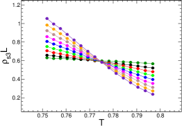
Figure 2: Monte Carlo data of $\rho_{s}L$ (top panel) and $\rho_{s3}L$ (bottom panel) for $J^{\prime}/J=3.5$. The lines are added to guide the eye.

observable	$J^{\prime}/J$	$T_{N}$	$J^{\prime}/J$	$T_{N}$
$\rho_{s}L$	2.5	1.0014(2)	3.5	0.7751(2)
$\rho_{s3}L$	2.5	1.0014(2)	3.5	0.7750(2)
$\rho_{s}L$	3.0	0.9317(2)	3.625	0.7087(3)
$\rho_{s3}L$	3.0	0.9316(2)	3.625	0.7086(3)
$\rho_{s}L$	3.25	0.8690(2)	3.75	0.6197(2)
$\rho_{s3}L$	3.25	0.8689(2)	3.75	0.6193(3)
$\rho_{s}L$	3.375	0.8270(2)	3.875	0.4853(3)
$\rho_{s3}L$	3.375	0.8269(2)	3.875	0.4849(4)

Table 1: The numerical values of $T_{N}$ at $J^{\prime}/J$ = 2.5, 3.0, 3.25, 3,375, 3.5, 3.625, 3.75, 3.875 determined by applying the leading scaling ansatz to the relevant observables. All the $\chi^{2}/{\text{DOF}}$ of these fits are smaller than 1.6.

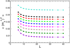
Figure 3: Monte Carlo data of $\langle(m_{s}^{z})^{2}\rangle$ as functions of $L$. From top to bottom the corresponding values of $J^{\prime}/J$ for these curves are 2.5, 3.0, 3.125, 3.25,…, 3.75, and 3.875, respectively. The lines are added to guide the eye.

Determination of the staggered magnetization density.— To calculate ${\cal M}_{s}$, we have measured the observable $\langle(m_{s}^{z})^{2}\rangle$. Specifically, by extrapolating the zero-temperature $\langle(m_{s}^{z})^{2}\rangle$ at finite lattice size to the bulk value $(m_{s}^{z})^{2}(\infty)$, ${\cal M}_{s}$ can then be obtained from ${\cal M}_{s}$ = $\sqrt{3(m_{s}^{z})^{2}(\infty)}$. Notice that to determine ${\cal M}_{s}$ by this method one needs the zero-temperature values of $\langle(m_{s}^{z})^{2}\rangle$. We have carried out trial runs for $L=20$ with $\beta J$ = 20 and $\beta J$ = 40 at $J^{\prime}/J$ = 2.5, 3.0, 3.125, 3.25, 3.375, 3.5, 3.625, 3.75, 3.875. The obtained values of $\langle(m_{s}^{z})^{2}\rangle$ for these two different inverse temperatures $\beta$ at all the considered couplings $J^{\prime}/J$ agree reasonably well. Hence the extrapolation using the data of $\langle(m_{s}^{z})^{2}\rangle$ calculated with $\beta J=L$ in the simulations should lead to correct results. Indeed it has been demonstrated in Ref. Jin12 that the extrapolated values of $\langle(m_{s}^{z})^{2}\rangle$ for various couplings $J^{\prime}/J$, determined with the data obtained from simulations employing $\beta J=L$ and $\beta J=2L$, are consistent with each other. Fig. 3 shows our $\langle(m_{s}^{z})^{2}\rangle$ data for $L=6,8,10,...,32,36,40$ at the considered $J^{\prime}/J$. The extrapolation results for these data using the ansatz $a+b/L+c/L^{2}+d/L^{3}$ are depicted in fig. 4. In fig. 4 the solid curve is reproduced from Ref. Oti12 and is the fitting result based on series expansion calculations. The agreement between our Monte Carlo data and series expansion results of ${\cal M}_{s}$ is remarkable.

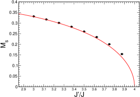
Figure 4: Monte Carlo determination of ${\cal M}_{s}$ as a function of $J^{\prime}/J$. The solid curve is reproduced from Ref. Oti12 and is the fitting result based on series expansion calculations.

Determination of the spinwave velocity.— There are several methods to determine the low-energy constant $c$. Here we use the idea of winding numbers squared. Specifically, for each $J^{\prime}/J$ we adjust the ratio of $L_{1}/L_{3}$ so that all three spatial winding numbers squared take approximately the same values. Then we tune $\beta$ in order to reach the condition $\langle W_{t}^{2}\rangle\sim\langle W_{i}^{2}\rangle$ for $i\in\{1,2,3\}$. Here $\langle W_{t}^{2}\rangle$ is the temporal winding number squared. Once this condition is met, the numerical value of $c$ is estimated to be $L/\beta_{2}\leq c\leq L/\beta_{1}$, where $L=(L_{1}L_{2}L_{3})^{1/3}$ and $\beta_{1}$ ($\beta_{2}$) stands for the largest (smallest) inverse temperature so that the criterion $\langle W_{i}^{2}\rangle\leq\langle W_{t}^{2}\rangle$ ($\langle W_{i}^{2}\rangle\geq\langle W_{t}^{2}\rangle$) for $i\in\{1,2,3\}$ is satisfied. For the isotropic case $J^{\prime}/J=1.0$, the spinwave theory predicts $c\sim 1.9091J$ Oit94 . Remarkably, for a trial simulation with $J^{\prime}/J=1.0$, $L_{1}$ = $L_{2}$ = $L_{3}$ = 20 and $\beta J=10.476$ (hence $L/\beta$ $\sim$ $1.9091J$), the ratio of the average of three spatial winding numbers squared and the temporal winding number squared is 0.994 approximately. This confirms the validity of calculating $c$ using the idea of winding numbers squared. For each coupling $J^{\prime}/J$ studied here, we further consider at least two sets of box sizes for which the condition $\langle W_{t}^{2}\rangle$ $\sim$ $\langle W_{i}^{2}\rangle$ for $i\in\{1,2,3\}$ is satisfied. With this strategy, the numerical values of $c$ obtained for $J^{\prime}/J$ = 2.5, 3.0, 3.25, 3.5, 3,375, 3.625, 3.75, 3.875, and 4.0 are shown in table 2. The results shown in table 2 imply that the values of $c$ at the considered couplings are already convergent to the corresponding bulk values. Even if some of our determined $c$ have not reached their bulk values, one expects the deviations to be very small. Hence such systematic uncertainty would have little impact on our investigation of the universal relation between $T_{N}$ and ${\cal M}_{s}$.

$J^{\prime}/J$	$L_{1}$	$L_{3}$	$c/J$	$J^{\prime}/J$	$L_{1}$	$L_{3}$	$c/J$
2.5	22	28	2.215(8)	3.5	46	62	2.348(10)
2.5	36	46	2.215(9)	3.625	22	30	2.360(12)
3.0	32	42	2.282(13)	3.625	34	46	2.360(13)
3.0	44	58	2.283(11)	3.75	22	30	2.376(12)
3.25	12	16	2.317(7)	3.75	44	60	2.378(11)
3.25	18	24	2.317(8)	3.875	16	22	2.391(7)
3.25	24	32	2.317(11)	3.875	32	44	2.389(8)
3.375	12	16	2.335(12)	4.0	16	22	2.408(13)
3.375	24	32	2.334(13)	4.0	32	44	2.405(15)
3.5	34	46	2.347(12)	4.0	42	58	2.401(10)

Table 2: The numerical values of $c$ obtained through the winding numbers squared for various couplings $J^{\prime}/J$

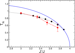
Figure 5: Results of $T_{N}$ as a function of $J^{\prime}/J$ determined by Monte Carlo simulations (solid circles), series expansion (solid squares) as well as field theory calculations (solid curve). The field theory and series expansion results are estimated and reproduced from Ref. Oti12 . The dashed and dotted lines are added to guide the eye.

Comparison between theoretical predictions and Monte Carlo results.— In Ref. Oti12 the following universal relation between $T_{N}$ and ${\cal M}_{s}$ near a QCP is predicted using the corresponding field theory

$$T_{N}=\sqrt{\frac{12c^{3}}{5}}{\cal M}_{s}.$$ (3)

Notice the original prediction in Ref. Oti12 has $c_{1}c_{2}c_{3}$ instead of $c^{3}$ for anisotropic systems. Here $c_{i}$ refers to the spinwave velocity in $i$ direction. On the other hand, considering the fact that both $T_{N}$ and ${\cal M}_{s}$ in Eq. (3) are bulk properties of the system for any given $J^{\prime}/J$, it is naturally to use the bulk spinwave velocity $c$ in the prediction. The use of $c$ in Eq. (3) is consistent with the way we determine this quantity. As we will demonstrate in the following, Eq. (3) is valid with our interpretation. To verify Eq. (3), in Ref. Oti12 the numerical values of $T_{N}$, $c$, and ${\cal M}_{s}$ for various couplings $J^{\prime}/J$ are determined numerically using the series expansion method. Further, the agreement between the numerical results from series expansion calculations and the field theory prediction is shown to be reasonably good. The quantum Monte Carlo determination of $T_{N}$ and ${\cal M}_{s}$ for the (3+1)-dimension ladder-dimer model is available in Ref. Jin12 as well. Notice that to quantitatively investigate the relation in Eq. (3), one needs to additionally calculate $c$. This motivates our study presented here. As a first step to quantitatively study Eq. (3), in fig. 4 we have already compared our Monte Carlo results for ${\cal M}_{s}$ with those determined by the series expansion method obtained in Ref. Oti12 . The consistency of ${\cal M}_{s}$ calculated with these two different methods is impressive. Next, we compare our Monte Carlo data of $T_{N}$ with the series expansion results available in Ref. Oti12 . Such a comparison is presented in fig. 5. Near the QCP $J^{\prime}/J\sim 0.4$, the consistency between the values of $T_{N}$ determined by these two different methods is reasonably good as well. Finally, Eq. (3) implies that the curve of $T_{N}/\sqrt{c^{3}}$ as a function of ${\cal M}_{s}$ should be linear assuming the logarithmic correction is not taken into account. In fig. 6 we compute $T_{N}/\sqrt{c^{3}}$ as a function of ${\cal M}_{s}$. Indeed qualitatively the curve shown in fig. 6 is linear in ${\cal M}_{s}$. A fit of the $T_{N}/\sqrt{c^{3}}$ data for $J^{\prime}/J=2.5,3.0,...,3.875$ in fig. 6 to the expression $a+b{\cal M}_{s}$ leads to $a=0.0117(20)$ which is slightly above the expected value $a=0$. We attribute such deviation to the logarithmic correction not taken into account in our analysis. Since the obtained $a=0.0117(20)$ is only slightly above zero, one expects that for the considered parameters $J^{\prime}/J$, either the effect due to the logarithmic correction is small or this correction only sets in significantly for the region with much stronger spatial anisotropy. Interestingly, the value of $b$ obtained from the fit is about half of the predicted value $\sqrt{12/5}$. This needs further investigation. One possible explanation is that we use $c^{3}$ instead of $c_{1}c_{2}c_{3}$ in Eq. (3). Without the explicit form of the logarithmic correction, we are not able to properly describe the data in our analysis. On the other hand, in the spirit of the expansion in chiral perturbation theory for Quantum Chromodynamics, it is naturally to include ${\cal M}_{s}\log({\cal M}_{s})$ as the additional correction. Remarkably, we can reach a good result using the ansatz $b_{1}{\cal M}_{s}+d_{1}{\cal M}_{s}\log({\cal M}_{s})$ for the fit (dashed line in fig. 6). Notice the resulting fitting curves of these two different ansätze match nicely in the regime where our Monte Carlo data are available.

Discussions and Conclusions.— In this report, we have simulated the three-dimensional ladder-dimer quantum Heisenberg model using the first principles Monte Carlo method. Our motivation is to investigate quantitatively the newly established universal relation between $T_{N}$ and ${\cal M}_{s}$ near a QCP. We find that for all the quantities considered here, such as $T_{N}$ and ${\cal M}_{s}$, our Monte Carlo calculations agree nicely with the corresponding results determined by the series expansion method. Assuming Eq. (3) is correct without considering the correction, then $T_{N}/\sqrt{c^{3}}$ as a function of ${\cal M}_{s}$ should vanish at ${\cal M}_{s}$ = 0. We find that the deviation between the extrapolated result of $T_{N}/\sqrt{c^{3}}$ and zero is of the order $10^{-2}$. This implies that either the logarithmic correction is small or this correction only sets in significantly for the region with much stronger spatial anisotropy. Indeed, our Monte Carlo data of $T_{N}/\sqrt{c^{3}}$ can be described well by an empirical ansatz $b_{1}{\cal M}_{s}+d_{1}{\cal M}_{s}\log({\cal M}_{s})$. Further, the resulting fitting curves of the two different ansätze used in our analysis match nicely in the regime where our Monte Carlo data are available. This confirms that indeed the logarithmic correction only sets in significantly for the region beyond what we have studied. Finally, using the spinwave theory and series expansion results available in Refs. Oit94 ; Oit04 , one obtains $T_{N}\sim 0.944$, ${\cal M}_{s}\sim 0.424$, and $c\sim 1.9091J$ for the isotropic case $J^{\prime}/J=1.0$. The data point of $T_{N}/\sqrt{c^{3}}$ and its corresponding ${\cal M}_{s}$ for $J^{\prime}/J=1.0$ is depicted as the square in fig. 6. It is remarkable that the prediction Eq. (3) is valid (qualitatively) all the way up to ${\cal M}_{s}\sim 0.4$.

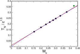
Figure 6: Monte Carlo data of $T_{N}/\sqrt{c^{3}}$ as functions of ${\cal M}_{s}$. While the solid line is the result of fitting the data to the form $a+b{\cal M}_{s}$, the dashed line is obtained using the ansatz $b_{1}{\cal M}_{s}+d_{1}{\cal M}_{s}\log({\cal M}_{s})$ for the fit. The square symbol stands for the result associated with $J^{\prime}/J=1.0$ and is obtained using the calculations in Refs. Oit94 ; Oit04 .

Partial support from NSC (Grant No. NSC 99-2112-M003-015-MY3) and NCTS (North) of R.O.C. is acknowledged. We appreciate greatly useful discussions with A. W. Sandvik and U.-J. Wiese.

References

- (1) V. Hinkov, P. Bourges, S. Pailhes, Y. Sidis, A. Ivanov, C. D. Frost, T. G. Perring, C. T. Lin, D. P. Chen, B. Keimer, Nature Physics 3, 780 (2007).
- (2) V. Hinkov et. al, Science 319, 597 (2008).
- (3) T. Pardini, R. R. P. Singh, A. Katanin and O. P. Sushkov, Phys. Rev. B 78, 024439 (2008).
- (4) S. Sachdev, C. Buragohain, and M. Vojta, Science 286, 2479 (1999).
- (5) M. Vojta, C. Buragohain, and S. Sachdev, Phys. Rev. B 61, 15152 (2000).
- (6) S. Sachdev, M. Troyer, and M. Vojta, Phys. Rev. Lett. 86, 2617 (2001).
- (7) M. Troyer, Prog. Theor. Phys. Supp. 145, 326 (2002).
- (8) Munehisa Matsumoto, Chitoshi Yasuda, Synge Todo, and Hajime Takayama, Phys. Rev. B 65, 014407 (2002)
- (9) K. H. Höglund and A. W. Sandvik, Phys. Rev. Lett. 91, 077204 (2003).
- (10) L. Wang, K. S. D. Beach, and A. W. Sandvik, Phys. Rev. B 73, 014431 (2006).
- (11) Kwai-Kong Ng and T. K. Lee, Phys. Rev. Lett. 97, 127204 (2006).
- (12) A. F. Albuquerque, M. Troyer, and J. Oitmaa, Phys. Rev. B 78, 132402 (2008).
- (13) Ch. Rüegg et al., Phys. Rev. Lett. 100, 205701 (2008).
- (14) Y. Kulik, and O. P. Sushkov, Phys. Rev. B 84, 134418 (2011).
- (15) J. Oitmaa, Y. Kulik, and O. P. Sushkov, Phys. Rev. B 85, 144431 (2012).
- (16) S. Jin and A. W. Sandvik, Phys. Rev. B 85, 020409(R) (2012).
- (17) A. W. Sandvik, Phys. Rev. B 66, R14157 (1999).
- (18) O. Nohadani, S. Wessel, and S. Haas, Phys. Rev. B 72, 024440 (2005).
- (19) J. Oitmaa, C. J. Hamer, and Zheng Weihong, Phys. Rev. B 50, 3877 (1994).
- (20) J. Oitmaa and Weihong Zheng, J. Phys.: Condens. Matter 16, 8653 (2004).