Monte Carlo determination of the critical exponents for a quantum phase transition of a dimerized spin-1/2 Heisenberg model

Abstract

We simulate the spin-1/2 Heisenberg model with a spatially staggered anisotropy using first principles Monte Carlo method. In particular, the critical exponents $\beta/\nu$ and $\omega$ associated with the quantum phase transition induced by dimerization are determined with high precision. Here $\beta$ and $\nu$ are the exponents related to the magnetization and the correlation length, respectively. In addition, $\omega$ is the confluent exponent. With very accurate data of the relevant observables, we first obtain a value of $\omega$ compatible with the known result in the $O(3)$ universality class. Further, using either the value of $\omega$ determined here or the established one in the literature, the exponent $\beta/\nu$ calculated from our data is in quantitative agreement with the known result $\beta/\nu=0.519(1)$ as well. Our investigation suggests that the quantum phase transition studied here is fully consistent with the $O(3)$ universality class.

I Introduction

Despite their simplicity, Heisenberg-type models continue to be one of the research topics in the condensed matter physics. With these models, one can obtain qualitative, or even quantitative understanding of real materials. It is also because of this feature of simplicity, various numerical methods are available to study the properties of Heisenberg-type models with high accuracy White92 ; White93 ; Schol05 ; Bea96 ; Evertz03 ; San97 ; San99 ; Proko98 ; Noack05 ; San10 ; Gull11 ; Troyer08 ; Bau11 . Indeed, by investigating these models with the various numerical methods, many theories, and consequently properties of real materials, are verified and better understood San95 ; Sac00 ; Tro02 ; Melin02 ; Hog03 ; Laf03 ; Lin03 ; Laf06 ; Hinkov2007 ; Hinkov2008 ; Pardini08 ; Jiang09.1 ; Rue08 ; Kul11 ; Oti12 ; Jin12 . Hence even those days, these simple models still have attracted a lot of theoretical interests. Among the studies of Heisenberg-type models carried out recently, one striking observation is the possibility of a new universality class for the two-dimensional dimerized spin-1/2 Heisenberg model with a spatially staggered anisotropy (2-d staggered-dimer model) Wenzel08 . It is believed that the quantum phase transition induced by dimerization of this model should be governed by the $O(3)$ universality class theoretically Chakr88 ; Haldane88 ; Chubu94 ; Sachdev99 ; Vojta03 . On the other hand, a recent large scale Monte Carlo calculation obtains $\nu=0.689(5)$ and $\beta/\nu=0.545(5)$ which are in contradiction to the established $O(3)$ results $\nu=0.7112(5)$ and $\beta/\nu=0.519(1)$ in the literature Cam02 . Here $\nu$ and $\beta$ are the critical exponents corresponding to the correlation length and the magnetization, respectively. Since this surprising finding, several efforts have been devoted to study the phase transition induced by dimerization of the 2-d staggered-dimer model. At the moment it is well-established theoretically that because of an irrelevant cubic term Fritz11 , there is a large correction to scaling for this phase transition which leads to the unexpected $\nu=0.689(5)$ and $\beta/\nu=0.545(5)$ obtained in Wenzel08 . Further, Monte Carlo study also provides strong evidence to support the scenario of an enhanced correction to scaling for this modelJiang11.8 .

While theoretically the unexpected results obtained in Wenzel08 can be explained by the cubic term introduced in Fritz11 , the explicit role of the cubic term is not clear at the moment. One natural explanation for the large correction to scaling due to the cubic term is the reduction of the magnitude of the confluent exponent $\omega$. Whether this is indeed the case has not explored yet. Hence in this study, we have investigated the phase transition induced by dimerization of the 2-d staggered-dimer spin-1/2 Heisenberg model on the square lattice. In particular, the numerical value of $\omega$ is determined with high precision. The exponent $\beta/\nu$ is also calculated as a by production. From our analysis, we find that our Monte Carlo data points are fully compatible with the established results $\omega=0.78(2)$ and $\beta/\nu=0.519(1)$ in the $O(3)$ universality class. Interestingly, while our Monte Carlo data for the considered model are consistent with the proposal of an enhanced correction to scaling due to an irrelevant cubic term, we find that the irrelevant cubic term likely has little influence on $\omega$. Hence the role of the cubic term for the large correction to scaling observed for the considered quantum phase transition requires further investigation.

This paper is organized as follows. First, after an introduction, the spatially anisotropic quantum Heisenberg model and the relevant observables studied in this work are briefly described in section two. Then in section three we present our numerical results. In particular, the results obtained from the finite-size scaling analysis are discussed in detail. Finally we conclude our investigation in section four.

Figure 1: The spatially anisotropic Heisenberg model considered in this study.

II Microscopic Model and Corresponding Observables

The Heisenberg model considered in this study is defined by the Hamilton operator

$$H=\sum_{\langle xy\rangle}J\,\vec{S}_{x}\cdot\vec{S}_{y}+\sum_{\langle x^{\prime}y^{\prime}\rangle}J^{\prime}\,\vec{S}_{x^{\prime}}\cdot\vec{S}_{y^{\prime}},$$ (1)

where $J$ ($J^{\prime}$) is the antiferromagnetic exchange coupling connecting nearest neighbor spins $\langle xy\rangle$ ($\langle x^{\prime}y^{\prime}\rangle$). The model described by Eq. (1) and investigated here is illustrated in fig. 1. To study the critical behavior of this model near the transition driven by the anisotropy, in particular to determine the confluent exponent $\omega$, the second Binder ratio $Q_{2}$ which is given by

$$Q_{2}=\frac{\langle(m_{s}^{z})^{2}\rangle^{2}}{\langle(m_{s}^{z})^{4}\rangle},$$ (2)

is calculated in our simulations. Here $m_{s}^{z}$ is the $z$ component of the staggered magnetization $\vec{m}_{s}=\frac{1}{L^{2}}\sum_{x}(-1)^{x_{1}+x_{2}}\vec{S}_{x}$. Notice the $L$ and $\vec{S}_{x}$ appearing above are the box sizes used in the calculations and a spin-1/2 operator at site $x$, respectively. In additional to $Q_{2}$, several generalized Binder ratios defined by

$$Q_{3} = \frac{\langle(m_{s}^{z})^{2}\rangle^{3}}{\langle(m_{s}^{z})^{6}\rangle},$$

$$Q_{31} = \frac{\langle(m_{s}^{z})^{2}\rangle\langle(m_{s}^{z})^{4}\rangle}{\langle(m_{s}^{z})^{6}\rangle}$$

$$Q_{8} = \frac{\langle(m_{s}^{z})^{4}\rangle^{2}}{\langle(m_{s}^{z})^{2}\rangle\langle(m_{s}^{z})^{6}\rangle},$$ (3)

are measured in our investigation as well. By carefully studying the spatial volume dependence of these Binder ratios at the critical point $(J^{\prime}/J)_{c}$, one can determine $\omega$ with high precision. Similarly, the exponent $\beta/\nu$ is calculated by studying the scaling behavior of the observables $\langle|m_{s}^{z}|\rangle$ and $\langle(m_{s}^{z})^{2}\rangle$ at $(J^{\prime}/J)_{c}$.

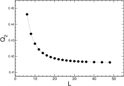
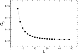
Figure 2: High accurate $Q_{2}$ (top panel) and $Q_{3}$ (bottom panel) data determined at $(J^{\prime}/J)_{c}=2.51950$ of the 2-d staggered-dimer model.

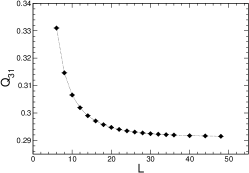
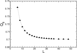
Figure 3: High accurate $Q_{31}$ (top panel) and $Q_{8}$ (bottom panel) data determined at $(J^{\prime}/J)_{c}=2.51950$ of the 2-d staggered-dimer model.

III The Numerical results

To determine $\beta/\nu$ and $\omega$, we have carried out large scale Monte Carlo simulations using the stochastic series expansion algorithm with operator-loop update San99 . Notice the calculations of $\beta/\nu$ and $\omega$ require precise knowledge of the critical point $(J^{\prime}/J)_{c}$. Specifically, at $(J^{\prime}/J)_{c}$ the expected finite-size scaling ansatz for $\langle|m_{s}^{z}|\rangle$ is given as Fisher72 ; Brezin82 ; Barber83 ; Brezin85 ; Fisher89

$$\langle|m_{s}^{z}|\rangle=(a+bL^{-\omega}+cL^{-2\omega})L^{-\beta/\nu},$$ (4)

where $a,\,b,\,c$ are some constants. Similarly, at the critical point, $\langle(m_{s}^{z})^{2}\rangle$ can be described quantitatively by

$$\langle(m_{s}^{z})^{2}\rangle=(a^{\prime}+b^{\prime}L^{-\omega}+c^{\prime}L^{-2\omega})L^{-2\beta/\nu},$$ (5)

here $a^{\prime},b^{\prime},c^{\prime}$ are again some constants. Finally, at $(J^{\prime}/J)_{c}$ the Binder ratios defined by Eq. (2) behave like

$$Q_{i}=(a_{i}+b_{i}L^{-\omega}+c_{i}L^{-2\omega})$$ (6)

with some constants $a_{i},\,b_{i},\,c_{i}$ as well.

The critical point $(J^{\prime}/J)_{c}$ of the considered phase transition has been calculated with high accuracy in Wenzel08 ; Jiang11.8 . Using the good scaling property of the observable winding number squared in the 2-direction, $(J^{\prime}/J)_{c}$ is estimated to be $2.51950(3)$ Jiang11.8 . Hence in our study, we have performed our simulations at $(J^{\prime}/J)_{c}=2.51950$ in order to determine the numerical values of $\omega$ and $\beta/\nu$. We have additionally carried out some calculations at $(J^{\prime}/J)_{c}=2.51953$ and $(J^{\prime}/J)_{c}=2.51947$ so that the systematic uncertainties for $\omega$ and $\beta/\nu$ due to the error of $(J^{\prime}/J)_{c}$ are properly taken into account. At $(J^{\prime}/J)_{c}=2.51950$ ($J^{\prime}/J=2.51953,2.51947$), the box sizes employed in our calculations range from $L=6$ to $L=48$ ($L=6$ to $L=40$). We use the relation $\beta J=4L$ is our simulations as well so that the validity of the finite-size scaling analysis performed here is guaranteed. Notice that very high precision related data points are essential to calculate $\omega$ accurately. Hence, for each $L$ at $J^{\prime}/J=2.51947$, $2.51950$, and $2.51953$, we have carried out at least 20 simulations. In particular, each simulation starts with different random seed and contains $2\times 10^{6}$ measurements. In other words, effectively each data is obtained with at least $4\times 10^{7}$ measurements. Finally, the estimators for $\langle|m_{s}^{z}|\rangle$ and $\langle(m_{s}^{z})^{k}\rangle$ with $k\geq 2$ as described in San97 are used in our calculations in order to reach a better statistic.

Observable	$L$	$\omega$	$\chi^{2}/{\text{DOF}}$
$Q_{2}$	$6\leq L\leq 48$	0.728(7)	1.2
$Q_{2}$	$6\leq L\leq 44$	0.726(8)	1.2
$Q_{2}$	$6\leq L\leq 40$	0.730(9)	0.93
$Q_{2}$	$6\leq L\leq 36$	0.729(10)	1.1
$Q_{2}$	$8\leq L\leq 48$	0.718(12)	0.93
$Q_{2}$	$8\leq L\leq 44$	0.710(15)	0.74
$Q_{2}$	$8\leq L\leq 40$	0.715(17)	0.7
$Q_{2}$	$8\leq L\leq 36$	0.709(20)	0.66
$Q_{2}$	$10\leq L\leq 48$	0.722(22)	0.98
$Q_{2}$	$10\leq L\leq 44$	0.707(27)	0.8
$Q_{3}$	$8\leq L\leq 48$	0.775(11)	1.05
$Q_{3}$	$8\leq L\leq 44$	0.773(13)	1.1
$Q_{3}$	$8\leq L\leq 40$	0.780(16)	0.86
$Q_{3}$	$8\leq L\leq 36$	0.780(18)	0.95
$Q_{3}$	$10\leq L\leq 48$	0.763(19)	0.93
$Q_{3}$	$10\leq L\leq 44$	0.754(24)	0.9

Table 1: The numerical values of $\omega$ calculated from $Q_{2}$ and $Q_{3}$ at $(J^{\prime}/J)_{c}=2.51950$ of the 2-d staggered-dimer model.

III.1 Determination of the exponent $\omega$

To determine $\omega$, let us focus on the finite-size scaling analysis of the Binder ratios defined by Eqs. (2) and (3). At the critical point, the finite-size scaling ansatz for all the observables $Q_{i}$ measured in our simulations are given by Eq. (6). Notice in addition to the corrections associated with the confluent exponent $\omega$, there are other subleading corrections with exponents $\omega^{\prime}>\omega$. Since the established values of $\omega^{\prime}$ are larger or equal to $2\omega$, it is reasonable to employ the scaling ansatz Eq. (6) for our data analysis. Notice one can define different Binder ratios using a similar manner. We find that the ones we define in Eqs. (2) and (3) have better scaling behavior and receive less corrections from higher order terms. Using the relevant data points at $(J^{\prime}/J)_{c}=2.51950$, tables one and two summarize the results of the fits associated with the determination of $\omega$. We have carried out many fits using data with different range of box sizes in order to understand how the value of $\omega$ converges with $L$. Notice all the errors quoted in this study are conservative estimates based on the uncertainties obtained directly from the fits. Although the numerical values of $\omega$ shown in tables one and two are slightly below the established $\omega=0.78(2)$ in the $O(3)$ universality class, they agree very well with $\omega=0.78(2)$ considering the fact that $\omega$ is a subleading exponent. Notice the Monte Carlo determination of $\omega$ presents in Has01 does not take into account the systematic uncertainties due to higher order corrections. In addition, while not being investigated systematically, it is interesting to observe that the values of $\omega$ determined in Has01 have a tendency of having smaller magnitude when data points of large $L$ are included in the fits. Hence one cannot rule out the scenario that indeed the true numerical value of $\omega$ in the $O(3)$ universality class is below $\omega=0.78(2)$ which is obtained using the series method Zinn98 . Nevertheless, the values of $\omega$ we reach here are in nice agreement with the well-established result $\omega=0.78(2)$. Finally to properly take into account the systematic error of $\omega$ due the the uncertainties of $(J^{\prime}/J)_{c}$, we have performed similar analysis for the data determined at $J^{\prime}/J=2.51947$ and $J^{\prime}/J=2.51953$. The related $Q_{2}$ and $Q_{3}$ ($Q_{31}$ and $Q_{8}$) data points obtained at $J^{\prime}/J=2.51947$ ($J^{\prime}/J=2.51953$) are presented in fig. 4 (fig. 5). Further, the results of these additional analysis are shown in tables 3 to 6. The results in tables 3 to 6 indicate that both the $\omega$ determined at these two values of $J^{\prime}/J$ are compatible with $\omega=0.78(2)$ as well. Notice the results associated with $J^{\prime}/J=2.51953$ have poor fitting quality compared to those of $J^{\prime}/J=2.51947$ and $J^{\prime}/J=2.51950$. This might due to either the impact from higher order corrections or the value $J^{\prime}/J=2.51953$ is slightly away from the true $(J^{\prime}/J)_{c}$. Considering the fact that both the fitting quality using the data determined with $J^{\prime}/J=2.51947$ and $J^{\prime}/J=2.51950$ are good, it is likely that $J^{\prime}/J=2.51953$ is not consistent with $(J^{\prime}/J)_{c}$ when the precision of our data is considered. Finally, using the results in tables 1 to 6 with absolute error $\leq$ 0.025 and $\chi^{2}/{\text{DOF}}\leq 2.0$, we arrive at $\omega\sim 0.738$. Here we do not quote the error for $\omega$ and it is reasonable to assume the error of $\omega$ is within 3 to 4 percent.

Observable	$L$	$\omega$	$\chi^{2}/{\text{DOF}}$
$Q_{31}$	$6\leq L\leq 48$	0.773(6)	2.8
$Q_{31}$	$6\leq L\leq 44$	0.775(7)	2.9
$Q_{31}$	$6\leq L\leq 40$	0.780(7)	2.35
$Q_{31}$	$6\leq L\leq 36$	0.782(8)	2.4
$Q_{31}$	$8\leq L\leq 48$	0.748(10)	0.83
$Q_{31}$	$8\leq L\leq 44$	0.745(12)	0.83
$Q_{31}$	$8\leq L\leq 40$	0.750(14)	0.7
$Q_{31}$	$8\leq L\leq 36$	0.748(16)	0.75
$Q_{31}$	$10\leq L\leq 48$	0.742(17)	0.85
$Q_{31}$	$10\leq L\leq 44$	0.733(22)	0.76
$Q_{8}$	$6\leq L\leq 48$	0.742(4)	1.7
$Q_{8}$	$6\leq L\leq 44$	0.743(5)	1.8
$Q_{8}$	$6\leq L\leq 40$	0.745(5)	1.6
$Q_{8}$	$6\leq L\leq 36$	0.746(6)	1.6
$Q_{8}$	$8\leq L\leq 48$	0.726(8)	0.55
$Q_{8}$	$8\leq L\leq 44$	0.724(10)	0.55
$Q_{8}$	$8\leq L\leq 40$	0.726(11)	0.54
$Q_{8}$	$8\leq L\leq 36$	0.725(13)	0.6
$Q_{8}$	$10\leq L\leq 48$	0.723(13)	0.57
$Q_{8}$	$10\leq L\leq 44$	0.718(17)	0.52
$Q_{8}$	$10\leq L\leq 40$	0.720(19)	0.54

Table 2: The numerical values of $\omega$ calculated from $Q_{31}$ and $Q_{8}$ at $(J^{\prime}/J)_{c}=2.51950$ of the 2-d staggered-dimer model.

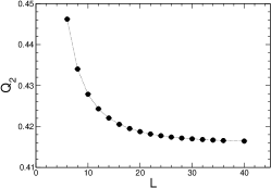
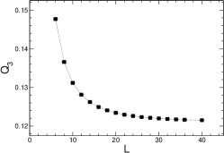
Figure 4: High accurate $Q_{2}$ (top panel) and $Q_{3}$ (bottom panel) data determined at $(J^{\prime}/J)_{c}=2.51947$ of the 2-d staggered-dimer model.

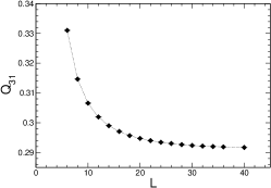
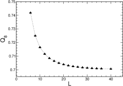
Figure 5: High accurate $Q_{31}$ (top panel) and $Q_{8}$ (bottom panel) data determined at $(J^{\prime}/J)_{c}=2.51953$ of the 2-d staggered-dimer model.

III.2 Determination of the exponent $\beta/\nu$

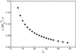
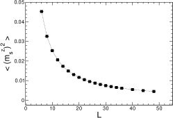
Figure 6: High precision data of $\langle|m_{s}^{z}|\rangle$ (top panel) and $\langle(m_{s}^{z})^{2}\rangle$ (bottom panel), obtained at $(J^{\prime}/J)_{c}=2.51950$, of the 2-d staggered-dimer model.

After having calculated the critical exponent $\omega$ from the relevant observables for the quantum phase transition induced by dimerization of the model described by fig. 1, we turn to the determination of the exponent $\beta/\nu$. To calculate $\beta/\nu$, the scaling behavior of the observables $\langle|m_{s}^{z}|\rangle$ and $\langle(m_{s}^{z})^{2}\rangle$ are studied. Specifically, at the critical point and for large $L$, the observable $\langle|m_{s}^{z}|\rangle$ and $\langle(m_{s}^{z})^{2}\rangle$ should scale according to Eqs. (4) and (5). Fig. 6 show our Monte Carlo data of $\langle|m_{s}^{z}|\rangle$ and $\langle(m_{s}^{z})^{2}\rangle$ determined at $(J^{\prime}/J)_{c}=2.51950$. In previous section, we demonstrate that the $\omega$ we obtain from several observables are in good agreement with $\omega=0.78(2)$. Hence, we have fixed $\omega=0.78$ in our analysis of determining $\beta/\nu$. We focus on applying the finite-size scaling analysis to the relevant data calculated at $(J^{\prime}/J)_{c}=2.51950$. The obtained values of $\beta/\nu$ are listed in tables 7 and 8. From tables 7 and 8, we conclude that the determined $\beta/\nu$ from our data with a fixed $\omega=0.78$ in the fits agree nicely with the established $\beta/\nu=0.519(1)$ known in the literature. Notice while the numerical values of $\omega$ we determine here are in good agreement with $\omega=0.78(2)$, they are slightly below $0.78$ with an average $0.738$. Interestingly, using a fixed $\omega=0.738$, the $\beta/\nu$ determined from the fits are in agreement with $\beta/\nu=0.519(1)$ as well. The results of these new fits using a fixed $\omega=0.738$ are shown in tables 7 and 8 as well. Interestingly, if we fixed $\beta/\nu$ to be 0.519 in Eqs. (4) and (5), then the values of $\omega$ obtained from the fits agree quantitatively with $0.78(2)$. For instance, applying the ansatz Eq. (4) (Eq. (5)) with a fixed $\beta/\nu=0.519$ to the observable $\langle|m_{s}^{z}|\rangle$ ($\langle(m_{s}^{z})^{2}\rangle$) for $8\leq L\leq 48$ leads to $\omega=0.779(9)$ ($\omega=0.753(7)$) with $\chi^{2}/{\text{DOF}}\sim 0.8$ ($\chi^{2}/{\text{DOF}}\sim 0.55$). In other words, our data of $\langle|m_{s}^{z}|\rangle$ and $\langle(m_{s}^{z})^{2}\rangle$ are fully compatible with $\beta/\nu=0.519(1)$ and $\omega=0.78(2)$ in the $O(3)$ universality class. Notice here the quoted errors of $\omega$ are the ones directly calculated from the fits. We have not attempted to performed a similar detailed analysis for the data obtained at $(J^{\prime}/J)=2.51947$ and $(J^{\prime}/J)=2.51953$. Considering the fact that $(J^{\prime}/J)_{c}$ is calculated to a very high accuracy, it is anticipated that the values of $\beta/\nu$ obtained from the data points calculated at $J^{\prime}/J=2.51947$ and $J^{\prime}/J=2.51953$ should be consistent with $\beta/\nu=0.519(1)$. We find that indeed this is the case Jiang13 . We also observe that the results obtained from the data associated with $J^{\prime}/J=2.51947$ have much better $\chi^{2}/{\text{DOF}}$ than those of $J^{\prime}/J=2.51953$. This provides another evidence that $J^{\prime}/J=2.51953$ is slightly away from the true critical point.

$J^{\prime}/J$	Observable	$L$	$\omega$	$\chi^{2}/{\text{DOF}}$
2.51947	$Q_{2}$	$6\leq L\leq 40$	0.717(9)	0.93
2.51947	$Q_{2}$	$6\leq L\leq 36$	0.719(11)	0.98
2.51947	$Q_{2}$	$6\leq L\leq 32$	0.717(12)	1.1
2.51947	$Q_{2}$	$8\leq L\leq 40$	0.702(18)	0.7
2.51947	$Q_{2}$	$8\leq L\leq 36$	0.701(22)	0.75
2.51947	$Q_{2}$	$8\leq L\leq 34$	0.693(24)	0.59
2.51947	$Q_{3}$	$8\leq L\leq 40$	0.768(17)	0.74
2.51947	$Q_{3}$	$8\leq L\leq 36$	0.771(20)	0.77
2.51947	$Q_{3}$	$8\leq L\leq 32$	0.764(24)	0.78
2.51947	$Q_{3}$	$10\leq L\leq 40$	0.748(32)	0.62

Table 3: The numerical values of $\omega$ calculated from $Q_{2}$ and $Q_{3}$ at $J^{\prime}/J=2.51947$ of the 2-d staggered-dimer model.

$J^{\prime}/J$	Observable	$L$	$\omega$	$\chi^{2}/{\text{DOF}}$
2.51947	$Q_{31}$	$6\leq L\leq 40$	0.772(8)	2.25
2.51947	$Q_{31}$	$6\leq L\leq 36$	0.777(9)	2.1
2.51947	$Q_{31}$	$6\leq L\leq 32$	0.779(11)	2.4
2.51947	$Q_{31}$	$8\leq L\leq 40$	0.740(16)	0.65
2.51947	$Q_{31}$	$8\leq L\leq 36$	0.742(19)	0.7
2.51947	$Q_{31}$	$8\leq L\leq 32$	0.733(22)	0.62
2.51947	$Q_{8}$	$6\leq L\leq 40$	0.741(6)	1.4
2.51947	$Q_{8}$	$6\leq L\leq 36$	0.744(7)	1.3
2.51947	$Q_{8}$	$6\leq L\leq 32$	0.744(8)	1.5
2.51947	$Q_{8}$	$8\leq L\leq 40$	0.722(12)	0.59
2.51947	$Q_{8}$	$8\leq L\leq 36$	0.724(15)	0.62
2.51947	$Q_{8}$	$8\leq L\leq 32$	0.715(18)	0.43

Table 4: The numerical values of $\omega$ calculated from $Q_{31}$ and $Q_{8}$ at $J^{\prime}/J=2.51947$ of the 2-d staggered-dimer model.

$J^{\prime}/J$	Observable	$L$	$\omega$	$\chi^{2}/{\text{DOF}}$
2.51953	$Q_{2}$	$6\leq L\leq 40$	0.732(10)	1.9
2.51953	$Q_{2}$	$6\leq L\leq 32$	0.745(13)	1.6
2.51953	$Q_{2}$	$8\leq L\leq 40$	0.711(20)	1.6
2.51953	$Q_{2}$	$8\leq L\leq 36$	0.718(24)	1.6
2.51953	$Q_{2}$	$8\leq L\leq 34$	0.726(27)	1.6
2.51953	$Q_{2}$	$8\leq L\leq 32$	0.733(30)	1.6
2.51953	$Q_{3}$	$6\leq L\leq 40$	0.832(9)	5.0
2.51953	$Q_{3}$	$6\leq L\leq 32$	0.856(12)	2.6
2.51953	$Q_{3}$	$8\leq L\leq 40$	0.777(18)	2.1
2.51953	$Q_{3}$	$8\leq L\leq 36$	0.789(22)	1.9
2.51953	$Q_{3}$	$8\leq L\leq 34$	0.800(25)	1.6
2.51953	$Q_{3}$	$8\leq L\leq 32$	0.809(27)	1.5
2.51953	$Q_{3}$	$10\leq L\leq 40$	0.759(33)	2.2

Table 5: The numerical values of $\omega$ calculated from $Q_{2}$ and $Q_{3}$ at $J^{\prime}/J=2.51953$ of the 2-d staggered-dimer model.

$J^{\prime}/J$	Observable	$L$	$\omega$	$\chi^{2}/{\text{DOF}}$
2.51953	$Q_{31}$	$6\leq L\leq 40$	0.785(8)	4.0
2.51953	$Q_{31}$	$6\leq L\leq 32$	0.803(11)	2.2
2.51953	$Q_{31}$	$8\leq L\leq 40$	0.747(16)	2.2
2.51953	$Q_{31}$	$8\leq L\leq 34$	0.767(22)	1.8
2.51953	$Q_{31}$	$8\leq L\leq 32$	0.775(25)	1.7
2.51953	$Q_{31}$	$10\leq L\leq 40$	0.736(30)	2.3
2.51953	$Q_{8}$	$6\leq L\leq 40$	0.748(6)	4.7
2.51953	$Q_{8}$	$6\leq L\leq 32$	0.763(8)	2.5
2.51953	$Q_{8}$	$8\leq L\leq 40$	0.723(12)	3.4
2.51953	$Q_{8}$	$8\leq L\leq 32$	0.748(17)	2.4
2.51953	$Q_{8}$	$10\leq L\leq 40$	0.718(22)	3.6
2.51953	$Q_{8}$	$10\leq L\leq 32$	0.785(40)	2.2

Table 6: The numerical values of $\omega$ calculated from $Q_{31}$ and $Q_{8}$ at $J^{\prime}/J=2.51953$ of the 2-d staggered-dimer model.

IV Discussion and Conclusion

In this study, we investigate the phase transition induced by dimerization for the staggered-dimer spin-1/2 Heisenberg model on the square lattice. In particular, we determine the values of the exponents $\omega$ and $\beta/\nu$ with high accuracy by employing the finite-size scaling analysis to the relevant observables. We find that both the numerical values of $\omega$ and $\beta/\nu$ determined here match very well with the established results $\omega\sim 0.78$ and $\beta/\nu=0.519(1)$ known in the literature. Our obtained $\omega$ has an average of $0.738$ which is slightly below $0.78$. Still, the agreement between our result $\omega\sim 0.738$ and $\omega\sim 0.78$ is reasonably well. Using either $\omega=0.738$ or $\omega=0.78$, the numerical values of $\beta/\nu$ determined in this study agree quantitatively with $\beta/\nu=0.519(1)$. The results reached here and those obtained in Jiang11.8 provide convincing evidence that the considered quantum phase transition is indeed governed by the $O(3)$ universality class. It is argued in Fritz11 that the large correction to scaling for the quantum phase transition induced by dimerization of the staggered-dimer model is due to an irrelevant cubic term. Our study find that the obtained $\omega$ is slightly below the predicted $\omega\sim 0.78$. This finding is consistent with the scenario that the cubic term influences the value of $\omega$. However, since the difference between our obtained $\omega$ and $\omega=0.78(2)$ is not significant, whether this is because of the cubic term needs a careful examination. Further, a slight reduction for the magnitude of $\omega$ cannot fully explain the large correction to scaling observed for the considered quantum phase transition. Finally, taking into account the fact that the numerical value of $\omega$ has not fully under control Has01 , it is desirable to carry out a more detailed investigation to examine the role of the cubic term for the quantum phase transition considered here. This will require a much precise value of $(J^{\prime}/J)_{c}$ than $(J^{\prime}/J)=2.51950(3)$ determined in Jiang11.8 and is beyond the scope of our study.

Observable	$L$	$\beta/\nu$	$\chi^{2}/{\text{DOF}}$
$\langle|m_{s}^{z}|\rangle$	$8\leq L\leq 48$	0.517(1)	0.95
$\langle|m_{s}^{z}|\rangle$	$8\leq L\leq 44$	0.5166(12)	0.81
$\langle|m_{s}^{z}|\rangle$	$8\leq L\leq 40$	0.5163(15)	0.84
$\langle|m_{s}^{z}|\rangle$	$10\leq L\leq 48$	0.5184(15)	0.6
$\langle|m_{s}^{z}|\rangle$	$10\leq L\leq 44$	0.5179(18)	0.56
$\langle|m_{s}^{z}|\rangle$	$10\leq L\leq 40$	0.5178(23)	0.62
$\langle|m_{s}^{z}|\rangle$	$8\leq L\leq 48$	0.5191(9)	0.8
$\langle|m_{s}^{z}|\rangle$	$8\leq L\leq 44$	0.5187(11)	0.7
$\langle|m_{s}^{z}|\rangle$	$10\leq L\leq 48$	0.5200(13)	0.56
$\langle|m_{s}^{z}|\rangle$	$10\leq L\leq 44$	0.5196(16)	0.55

Table 7: The numerical values of $\beta/\nu$ calculated from $\langle|m_{s}^{z}|\rangle$ of the 2-d staggered-dimer model a fixed $\omega=0.738$ (the top six rows) and a fixed $\omega=0.78$ (the bottom four rows) for the fits.

Observable	$L$	$\beta/\nu$	$\chi^{2}/{\text{DOF}}$
$\langle(m_{s}^{z})^{2}\rangle$	$8\leq L\leq 48$	0.5183(10)	0.6
$\langle(m_{s}^{z})^{2}\rangle$	$8\leq L\leq 44$	0.5180(12)	0.55
$\langle(m_{s}^{z})^{2}\rangle$	$8\leq L\leq 40$	0.5178(15)	0.58
$\langle(m_{s}^{z})^{2}\rangle$	$10\leq L\leq 48$	0.5191(14)	0.48
$\langle(m_{s}^{z})^{2}\rangle$	$10\leq L\leq 44$	0.5187(18)	0.49
$\langle(m_{s}^{z})^{2}\rangle$	$10\leq L\leq 40$	0.5187(23)	0.53
$\langle(m_{s}^{z})^{2}\rangle$	$8\leq L\leq 48$	0.5204(9)	0.49
$\langle(m_{s}^{z})^{2}\rangle$	$8\leq L\leq 44$	0.5202(11)	0.49
$\langle(m_{s}^{z})^{2}\rangle$	$10\leq L\leq 48$	0.5208(13)	0.46
$\langle(m_{s}^{z})^{2}\rangle$	$10\leq L\leq 44$	0.5206(16)	0.48

Table 8: The numerical values of $\beta/\nu$ calculated from $\langle(m_{s}^{z})^{2}\rangle$ of the 2-d staggered-dimer model with a fixed $\omega=0.738$ (the top six rows) and a fixed $\omega=0.78$ (the bottom four rows) for the fits.

V Acknowledgments

Partial support from NSC and NCTS (North) of R.O.C. is acknowledged.

References

- (1) S. R. White, Phys. Rev. Lett. 69, 2863 (1992)
- (2) S. R. White, Phys. Rev. B 48, 10345 (1993).
- (3) U. Schollwöck, Rev. Mod. Phys. 77, 259 (2005).
- (4) B. B. Beard and U.-J. Wiese, Phys. Rev. Lett. 77, 5130 (1996).
- (5) H. G. Evertz, Adv. Phys. 52, 1 (2003).
- (6) A. W. Sandvik, Phys. Rev. B (1997).
- (7) A. W. Sandvik, Phys. Rev. B 66, R14157 (1999).
- (8) N. V. Prokofév, B. V. Svistunov, I. S. Tupitsyn, Phys. Lett. A 238, 253 (1998),
- (9) Reinhard M. Noack, Salvatore R. Manmana, AIP Conf. Proc. 789, 93 (2005).
- (10) A. W. Sandvik, AIP Conf. Proc. 1297, 135 (2010).
- (11) E. Gull, A. J. Millis, A. I. Lichtenstein, A. N. Rubtsov, M. Troyer and P. Werner, Rev. Mod. Phys. 83, 349–404 (2011).
- (12) A. F. Albuquerque et. al, Journal of Magnetism and Magnetic Material 310, 1187 (2007).
- (13) B. Bauer et al. (ALPS collaboration), J. Stat. Mech. P05001 (2011).
- (14) A. W. Sandvik and M. Vekic, Phys. Rev. Lett. 74, 1226 (1995).
- (15) S. Sachdev, C. Buragohain, and M. Vojta, Science 286, 2479 (1999); M. Vojta, C. Buragohain, and S. Sachdev, Phys. Rev. B 61, 15152 (2000).
- (16) M. Troyer, Prog. Theor. Phys. Supp. 145, 326 (2002).
- (17) R. Melin, Y.-C. Lin, P. Lajko, H. Rieger, and F. Iglói, Phys. Rev. B 65, 104415 (2002).
- (18) K. H. Höglund and A. W. Sandvik, Phys. Rev. Lett. 91, 077204 (2003).
- (19) Nicolas Laflorencie and H. Rieger, Phys. Rev. Lett. 91, 229701 (2003).
- (20) Y. C. Lin, H. Rieger, and F. Iglói, Phys. Rev. B 68, 024424 (2003).
- (21) Nicolas Laflorencie, Stefan Wessel, andreas Läuchli, and Heiko Rieger, Phys. Rev. B 73, 060403(R) (2006).
- (22) V. Hinkov, P. Bourges, S. Pailhes, Y. Sidis, A. Ivanov, C. D. Frost, T. G. Perring, C. T. Lin, D. P. Chen, B. Keimer, Nature Physics 3, 780 (2007).
- (23) V. Hinkov et. al, Science 319, 597 (2008).
- (24) T. Pardini, R. R. P. Singh, A. Katanin and O. P. Sushkov, Phys. Rev. B 78, 024439 (2008).
- (25) F.-J. Jiang, F. Kämpfer, and M. Nyfeler, Phys. Rev. B 80, 033104 (2009).
- (26) Ch. Rüegg et al., Phys. Rev. Lett. 100, 205701 (2008).
- (27) Y. Kulik, and O. P. Sushkov, Phys. Rev. B 84, 134418 (2011).
- (28) J. Oitmaa, Y. Kulik, and O. P. Sushkov, Phys. Rev. B 85, 144431 (2012).
- (29) S. Jin and A. W. Sandvik, Phys. Rev. B 85, 020409(R) (2012).
- (30) S. Wenzel, L. Bogacz, and W. Janke, Phys. Rev. Lett. 101, 127202 (2008).
- (31) S. Chakravarty, B. I. Halperin, and D. R. Nelson, Phys. Rev. Lett. 60, 1057 (1988).
- (32) F. D. M. Haldane, Phys. Rev. Lett. 61, 1029 (1988).
- (33) A. V. Chubukov, S. Sachdev, and J. Ye, Phys. Rev. B 49, 11919 (1994).
- (34) S. Sachdev, Quantum Phase Transitions (Cambridge University Press, Cambridge, 1999).
- (35) M. Vojta, Rep. Prog. Phys. 66, 2069 (2003).
- (36) M. Campostrini, M. Hasenbusch, A. Pelissetto, P. Rossi, and E. Vicari, Phys. Rev. B 65, 144520 (2002).
- (37) L. Fritz et al., Phys. Rev. B 83, 174416 (2011).
- (38) F.-J. Jiang, Phys. Rev. B 85 014414 (2012).
- (39) M. E. Fisher and M. N. Barber, Phys. Rev. Lett. 28, 1516 (1972).
- (40) E. Brézin, J. Phys. (Paris) 43, 15 (1982).
- (41) M. N. Barber, in Phase Transitions and Critical Phenomena, ed. C. Domb (Academic, New York, 1983), Vol. 8.
- (42) E. Brézin and J. Zinn-Justin, Nucl. Phys. B 257, 867 (1985).
- (43) M. P. A. Fisher, P. B. Weichman, G. Grinstein, and D. S. Fisher, Phys. Rev. B 40, 546 (1989).
- (44) M. Hasebbusch, J. Phys. A: Math. Gen. 34 (2001) 8221.
- (45) R. Guida and J. Zinn-Justin, J. Phys. A: Math. Gen. 31 (1998) 8103.
- (46) F.-J. Jiang, unpublished.